| Issue |
A&A
Volume 678, October 2023
|
|
|---|---|---|
| Article Number | A122 | |
| Number of page(s) | 14 | |
| Section | Cosmology (including clusters of galaxies) | |
| DOI | https://doi.org/10.1051/0004-6361/202347191 | |
| Published online | 12 October 2023 | |
Investigating the outskirts of Abell 133 with Suzaku and Chandra observations⋆
1
SRON Netherlands Institute for Space Research, Niels Bohrweg 4, 2333 CA Leiden, The Netherlands
e-mail: Z.Zhu@sron.nl
2
Leiden Observatory, Leiden University, Niels Bohrweg 2, 2300 RA Leiden, The Netherlands
3
Department of Theoretical Physics and Astrophysics, Faculty of Science, Masaryk University, Kotlárská 2, 61137 Brno, Czech Republic
4
Kavli Institute for the Physics and Mathematics of the Universe, The University of Tokyo, Kashiwa, Chiba, 277-8583
Japan
Received:
14
June
2023
Accepted:
1
August
2023
Context. Past observations and simulations have predicted an increasingly inhomogeneous gas distribution towards the outskirts of galaxy clusters. However, the exact properties of such gas clumping are not yet well known. The outskirts of Abell 133 can benefit from deep X-ray observations, with a 2.4 Ms ultra-deep Chandra exposure, as well as eight archival Suzaku pointings, making it a unique laboratory for studying the clumping of the intracluster medium (ICM).
Aims. We searched for significant clump candidates with the specific aim of identifying ones that could represent genuine ICM inhomogeneity. To further understand how clumping biases the thermodynamic profiles, we compared the measurements including and excluding the clump candidates.
Methods. We jointly analyzed Chandra and Suzaku observations of Abell 133. We selected clump candidates with at least 2σ significance based on the Chandra image and we discussed their origins further, using information from the DESI Legacy Imaging Surveys cluster catalog as well as the CFHT r-band image. We performed multiple rounds of Suzaku spectral analysis with different corrections for the underlying point sources and clump distribution and we compared the resulting thermodynamic profiles.
Results. We detected 16 clump candidates using Chandra, most of which are identified as background clusters or galaxies – as opposed to intrinsic inhomogeneity. Even after the correction of the resolved clumps, the entropy profile approaching the outskirts still flattens, deviating from the power law model expected from self-similar evolution, which implies that unresolved clumping and other complex physics contribute to the entropy flattening in the outskirts.
Key words: Galaxies: clusters: intracluster medium / Galaxies: clusters: individual: Abell 133 / X-rays: galaxies: clusters
Reduced images are available at the CDS via anonymous ftp to cdsarc.cds.unistra.fr (130.79.128.5>) or via https://cdsarc.cds.unistra.fr/viz-bin/cat/J/A+A/678/A122
© The Authors 2023
 Open Access article, published by EDP Sciences, under the terms of the Creative Commons Attribution License (https://creativecommons.org/licenses/by/4.0), which permits unrestricted use, distribution, and reproduction in any medium, provided the original work is properly cited.
This article is published in open access under the Subscribe to Open model. Subscribe to A&A to support open access publication.
1. Introduction
The properties of the intracluster medium (ICM) in the outskirts of galaxy clusters have been actively explored with a combination of multi-wavelength observations and state-of-the-art numerical simulations (for a review, see Walker et al. 2019). These outer regions of galaxy clusters are an ideal probe of the ongoing process of virialization due to large-scale structure growth. Both predictions from numerical simulations and observational studies indicate that cluster outskirts exhibit distinct marks of recent accretion from the surrounding large-scale structure, for instance: an inhomogeneous gas density distribution (Simionescu et al. 2011; Nagai & Lau 2011), non-thermal pressure (Ghirardini et al. 2018; Nelson et al. 2014), and non-equilibrium electrons in the ICM (Hoshino et al. 2010; Avestruz et al. 2015). An increase of the gas clumping at larger radii can lead to significant systematic biases in the X-ray measurements of various ICM properties, for instance, leading to overestimations of the density and, consequently, underestimations of the gas entropy. Although this effect has been invoked in numerous works to explain why the observed entropy profiles deviate from the expected baseline derived from pure gravitational heating (e.g., Walker et al. 2013; Urban et al. 2014; Tchernin et al. 2016; Simionescu et al. 2017), as mentioned above, several other physical effects can simultaneously be at play in addition to the gas clumping. Only deep observations offering both sharp imaging and reliable spectral information of these faint regions can help us to truly disentangle the complex physics of cluster outskirts.
To date, Chandra has accumulated ultra-deep exposures on Abell 133 and Abell 1795, out to very large radii, providing a special coverage in the outskirts even beyond r200. Suzaku observations offer a similar coverage out to r200, enabling us to directly measure the thermodynamic properties owing to the relatively low and stable background. This unique combination of available data makes these clusters ideal probes for understanding the complex physics of the ICM near the virial radii.
Abell 133 is an X-ray luminous cool-core galaxy cluster at z = 0.0566 (Struble & Rood 1999), which has a cool core and a central radio source. Previous Chandra studies with relatively shallow exposure (Fujita et al. 2002; Randall et al. 2010) showed that the cluster core of Abell 133 has a complex morphology and prominent radio relics indicative of ongoing merger activity. Using the 2.4 Ms deep Chandra observations, Vikhlinin (2013) reported the detection of three X-ray filaments extending outside of r200. To verify this claim, Connor et al. (2018) conducted a spectrographic campaign on the Baade 6.5 m telescope around Abell 133 and found corresponding galaxy enhancements along those filaments. With this ultra-deep dataset, Morandi & Cui (2014) have shown that clumping increases with radius, however, they did not study the nature of individual clumps.
In this paper, we report on results from a combined X-ray analysis using Chandra and Suzaku observations of Abell 133. To precisely correct the thermodynamic profiles for this gas clumping effect, we attempted to identify significant clumps based on Chandra images and mask them in the Suzaku spectral analysis. We introduce the imaging analysis in Sect. 3 and present surface brightness profiles in Sect. 4. We list the 16 Chandra-selected clump candidates in Sect. 5 and discuss their origins. Our Suzaku spectral analysis methods are described in Sect. 6. Section 7 shows the resulting thermodynamic profiles. Furthermore, in Sect. 8, we discuss how the profiles are affected by clumping corrections, as well as other systematic uncertainties which can be mitigated owing to the combination of Chandra and Suzaku coverage. In a companion paper (Kovács et al. 2023), we applied the same techniques for Abell 1795 and discussed the corresponding results. In this work, we adopt a ΛCDM cosmology with Ωm = 0.27 and H0 = 70 km s−1 Mpc−1. This gives a physical scale 1′ = 64.2 kpc for A133 cluster at redshift z = 0.0566. Our reference values for r500 and r200 are 14.6′ and 24.7′, respectively (Randall et al. 2010). All errors are given at the 68% confidence level unless otherwise stated.
2. Observations and data reduction
2.1. Suzaku
We utilized eight Suzaku observations mapping the Abell 133 cluster to 1.2r200. The four observations (E, S, N, and W) pointing to the inner core region have been studied in Ota & Yoshida (2016), while the later observations towards the outskirts have not yet been explored thus far. Detailed information on these observations can be found in Table 1.
Suzaku observational log.
The X-ray Imaging Spectrometer(XIS) data were analyzed following the procedure described in Simionescu et al. (2013), Urban et al. (2014) and Zhu et al. (2021). In brief, we used the cleaned events files produced by the standard screening process1, and applied the following additional filtering criteria. The observation periods with low geomagnetic cut-off rigidity (COR ≤ 6 GV) were excluded. For observations later than 2011, we excluded two columns on either side of the charge-injected columns for the XIS1 detector to avoid the charge leak effect. The vignetting effect was corrected using ray-tracing simulations of extended, spatially uniform emission. The data reduction was performed with HEAsoft v6.26. We have examined the 0.7–3 keV light curves of each observation with a time bin of 256 seconds, to further ensure no flaring occurred during the clean exposure. In addition, we checked for potential contamination from solar wind charge exchange (SWCX), by plotting the proton flux measured by the WIND spacecraft’s solar wind experiment instrument2, as shown in Fig. A.1. We found the proton flux curves of the eight observations are much lower than 4 × 108 cm−2 s−1, therefore, the contamination from geocoronal SWCX is negligible (Yoshino et al. 2009).
2.2. Chandra
Abell 133 was frequently observed by Chandra’s Advanced CCD Imaging Spectrometer (ACIS) from 2002 to 2019. We utilized 38 observations taken in ACIS-I VFAINT mode, which accumulated to a total of 2.26 Ms clean exposure (see Table 2).
Chandra observational log.
All data were reprocessed using the CIAO data analysis package (version 4.13) and the latest calibration database (CALDB 4.9.4) distributed by the Chandra X-ray Observatory Center. We removed the cosmic rays and bad pixels from all level-1 event files using the CIAO tool chandra_repro with VFAINT mode background event filtering. For each observation, we extracted the lightcurve in the 9–12 keV band, to examine possible contamination from flare events. To remove the time intervals with anomalous background, we applied the CIAO tool deflare to filter out the times where the background rates exceed ±2σ of the average value.
We utilized stowed background files to estimate the non-X-ray background (NXB). All stowed background events files were combined and reprocessed with acis_process_events using the latest gain calibration files. For each observation, we scaled the NXB to match the 9–12 keV count rate of the observation.
3. X-ray imaging
3.1. Suzaku
We extracted images from all three XIS detectors in the 0.7–7 keV band and removed a 30″ region around the detector edges. To minimize the influence of systematic uncertainties related to the vignetting correction, pixels with an effective area less than half of the on-axis value were also masked. Using night Earth observations, we generated the corresponding instrumental background images. Vignetting effects were corrected after background subtraction using ray-tracing simulations of extended, spatially uniform emission. Figure 1 shows the resulting flux image of Abell 133, smoothed with a Gaussian kernel of 25″. We identified nine point sources based on the Suzaku image, which are shown in Fig. B.1.
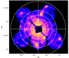 |
Fig. 1. Exposure- and vignetting-corrected 0.7–7 keV Suzaku image of Abell 133. The 90-degree white annuli show extraction regions applied in the spectral analysis. |
3.2. Chandra
We extracted and combined the 0.5–3 keV count images using merge_obs. Background images were generated from the stowed observation files described in Sect. 2. We calculated the exposure maps using a weighted spectrum file generated by make_instmap_weighted, where the spectral model is an absorbed apec model with kT = 3 keV, which is the average temperature measured by previous Chandra studies (Vikhlinin et al. 2005). After correcting the NXB-subtracted count image with the combined exposure map, we obtained the Chandra flux map. A contour-binning algorithm (Sanders 2006) was then applied to this flux map to create a binned image with each bin reaching a signal-to-noise ratio (S/N) of 3 (see Fig. 2).
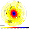 |
Fig. 2. Contour binned image of the inner 30′ of Abell 133 in the 0.5–3 keV energy band. The point sources detected by wavdetect have been removed. Each bin has a S/N ≥ 3, and an average photon flux as indicated by the color bar in units of photon cm−2 s−1 pixel−1. Here, 1 pixel corresponds to 0.98″. |
We employed the wavdetect algorithm on the combined counts images in the 0.5–3 keV band, adopting a false-positive probability threshold of 10−6 and wavelet scales of 1, 2, 4, 8, 16, 32, and 64 pixels. A merged 90% Enclosed Counts Fraction (ECF) psfmap and merged exposure map generated by merge_obs were supplied to the detection process. A total of 1175 point sources were identified and then excluded from the following analysis. Utilizing the same Chandra dataset, Shin et al. (2018) showed that the cumulative number count distribution (i.e., logN-logS curve) in Abell 133 is consistent with the CDF-S field Lehmer et al. (2012) within 1σ uncertainty. This indicates that no explicit excess in the outskirts was observed, due to unidentified clumps among wavdetect sources.
4. Surface brightness profile
The azimuthally averaged surface brightness profiles of Abell 133 were extracted and fitted with the pyproffit package by Eckert et al. (2011). In accordance with the analysis described in Sect. 5, both Chandra and Suzaku surface brightness profiles were fitted only in the outskirts, from 10.2′ (r500) to 30′. Before extraction, we first excluded the point sources above a photon flux threshold of 2 × 10⁻⁶ photon cm−2 s−1, using the Chandra source list from wavdetect (see Sect. 3.2). We extracted concentric annuli centered on the X-ray peak of Abell 133 (J2000 (RA, Dec) = (15.67333, −21.88011); Randall et al. 2010) and binned the Chandra profile using a width of 2′, while for Suzaku, a bin size of 3′ was applied to account for its larger PSF size.
We fit the extracted surface brightness profiles with a power-law model (pyproffit.PowerLaw), Sx = S0(r/r0)−α + B, where B represents the sky background. Compared to the commonly used β-model, our best-fit power-law models give a better description for the outskirts of Abell 133, since the β parameter and core radius (r0) of the β-model are strongly coupled outside the fitted radii (Mohr et al. 1999).
In Fig. 3, we show the background-subtracted surface brightness profiles with best-fit power-law models in units of erg s−1 cm−2 deg−2. The energy flux is converted from the photon flux with the same spectral model assumed in Sect. 3.2. The best-fit power-law indices are in good agreement, namely, α = 4.37 ± 0.24 and α = 4.10 ± 0.60 for Chandra and Suzaku, respectively, indicating the two profiles are well consistent.
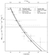 |
Fig. 3. 0.5–3 keV background-subtracted azimuthally averaged surface brightness profile of the outskirts of Abell 133 obtained from Chandra (black) and Suzaku (grey) data with the corresponding best-fit power-law models overplotted. The Suzaku sky background level is relatively higher compared to Chandra, which reflects the excess emission from Chandra-selected point sources whose PSF is broader than the source extraction region. |
5. Clumping
Zhuravleva et al. (2013) presented a useful method to characterize the ICM inhomogeneity. Their work showed that the gas density in a given annulus roughly follows a log-normal distribution, while a high-density tail can be seen as a result of gas clumping. In such a case, the mean and the median values of the distribution separate, as the median coincides with the peak of the log-normal profile and the mean shifts to a higher density. As the X-ray emission is proportional to the square of the local density, it has been indicated by previous work that a similar distribution is also found for the surface brightness and flux (Eckert et al. 2015; Mirakhor & Walker 2021).
In the Chandra image, two large, bright clumps are immediately evident in the southeast (labelled BC1 and BC2). To search for additional clumps, we examine the surface brightness distribution of 4 annuli divided from 10.2′ (0.7r500) to 30′ in Fig. 4. The ICM of the inner core region within 0.7r500 is affected by sloshing and merging events and, more importantly, we are mainly focused on the outskirts. Therefore we only search for clump candidates outside of 0.7r500. We fit each distribution with a log-normal profile and obtain the best-fit centroid and sigma. For each annulus, the median flux coincides well with the fit centroid, while the mean flux is shifted towards the high flux end, indicating an asymmetric distribution with a high-flux tail. To quantify this asymmetry, we calculated the Fisher-Pearson coefficient of skewness of the distributions and estimated its 1-σ error range using a bootstrap method with 105 resamplings. The skewness measurements, along with other surface brightness distribution parameters, are listed in Table 3. We notice that the skewness is positive in each annulus and roughly presents an increasing trend towards larger radii. We note that in the outermost annulus, the presence of BC1 and BC2 would dominate and distort the formal log-normal profile (see Fig. 4) and, therefore, these have been excluded from the calculation of the median and skewness. We selected 2σ outliers from the surface brightness distribution of each annulus and then localized them on the adaptively-binned image. We further merged neighbouring outlier bins and identified 16 clump candidates, which are listed in Table 4. In case several neighboring outlier bins were combined into a single clump, their individual significances were added in quadrature. More details and tests for the X-ray clumping detection can be found in Kovács et al. (2023).
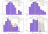 |
Fig. 4. 0.5–3 keV surface brightness distribution of Abell 133 outskirts obtained in 4 annuli, mapping from 10.2′ to 30.0′ as listed in Table 3. The histogram in grey shows the contribution from the large, bright diffuse features in the southeast, which have been excluded from further analysis. The solid orange line marks the 2σ outlier threshold. |
Surface brightness distribution parameters.
Clump candidates.
Combining the cluster catalog from the DESI Legacy Imaging Surveys (Zou et al. 2021) and the r-band CFHT image taken as part of the Multi-Epoch Nearby Cluster Survey (Sand et al. 2012; Graham et al. 2012), we discuss the origin of individual clump candidates below.
– BC1: overlaps with a large, bright background cluster (z ∼ 0.46).
– BC2: overlaps with a large, bright background cluster (z ∼ 0.23).
– C3: the diffuse emission might be contributed from the nearby X-ray point source 2CXOJ010320.8-213317, although its X-ray luminosity is relatively low, namely, S0.5 − 7 ≤ 3.85 × 10⁻¹⁵ erg s−1 cm−2.
– C4: the candidate overlaps with a background cluster at the redshift of z ∼ 0.63.
– C5: this candidate is adjacent to the X-ray point source 2CXO J010313.9-214103; however, its flux is weak (S2 − 7 ≤ 1.76 × 10⁻¹⁵ erg s−1 cm−2). Therefore, the observed diffuse emission is not likely to originate from this point source. Within the contour, there is also a member galaxy (z ∼ 0.076 + −0.027). However, the most likely origin of the surface brightness excess is an overdensity of galaxies with redshifts between 0.3 to 0.6, which are concentrated at the place where diffuse X-ray emission has been found.
– C6: this candidate picks the emission from a weak point source 2CXO J010346.5-214653 (S2 − 7 = 2.50 × 10⁻¹⁵ erg s−1 cm−2), which is missed by our point source detection.
– C7: this is one of the nearest candidates to the core of Abell 133, which might hint to real ICM enhancement due to sloshing or feedback in the cluster core.
– C8: overlaps with a background cluster at the redshift of z ∼ 0.66.
– C9: located at the boundary of a background cluster (z ∼ 0.61). A concentration of background galaxies overlaps our candidate clump.
– C10: a weak X-ray point source CXOGSG J010134.1-213943 (Wang et al. 2016), with a luminosity of L0.3 − 8 ∼ 5.8 × 1040 erg s−1.
– C11: overlaps with a background cluster (z ∼ 0.41). Although the brightest parts of the diffuse emission are removed as point sources, the remaining emission has been picked out by our method.
– C12: overlaps with a background cluster at the redshift of z ∼ 0.72.
– C13: this candidate close to the core region of Abell 133 could also be real ICM enhancement due to sloshing or feedback in the cluster core.
– C14: same as C7 and C13.
– C15: overlaps with a galaxy WISEA J010204.45-220515.2. This candidate is identified as a very weak X-ray point source in Shin et al. (2018), with flux of S0.5 − 2 = 2.70 × 10⁻¹⁶ erg s−1 cm−2.
– C16: the X-ray peak of this candidate on the upper right corner, coincides with the galaxy WINGS J010146.15-220225.2 (Varela et al. 2009).
We plot the cut-out images of Chandra and CFHT for each selected clump candidate in Fig. 5, using an image size of 0.2 Mpc × 0.2 Mpc, for better visual comparison. The physical sizes of the clumps range from 8 kpc to ∼90 kpc in radius. In conclusion, most of our clump candidates are background clusters or galaxies (BC1, BC2, C4, C5, C8, C9, C11, C12, and C16), some are weak point sources missing from the source detection (C6, C10, and C15), and the rest need further exploration (C3, C7, C13, and C14).
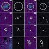 |
Fig. 5. 0.5–3 keV cut-out images for clump candidates (white regions). Left: Each Chandra image has a size of 200″ × 200″ (0.2 Mpc × 0.2 Mpc) and is smoothed with a Gaussian function with a kernel of 6 pixels. Filled black ellipses represent excluded wavdetect sources. The orange dashed circles mark the r500 radius of background clusters (Zou et al. 2021). Right:r-band CFHT image showing the same field of view. |
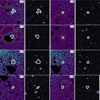 |
Fig. 5. continued. |
We followed the definition of the emissivity bias, bx, from Eckert et al. (2015), where bx = SBmean/SBmedian, to check the difference before and after removal of our identified clumps. For each annulus, we used the mean and median surface brightness of bins within this annulus for SBmean and SBmedian. In Fig. 6, we plot the azimuthally averaged emissivity bias profiles with and without the resolved clumps, where we see a difference beyond r500. We emphasize that the difference in the outermost annulus is underestimated since two bright clumps (BC1 and BC2) were excluded prior to the clumping analysis. We further compare the measurements of Abell 133 with the average emissivity bias profile measured from 31 clusters in the redshift range 0.04 ∼ 0.2 observed with the ROSAT/Position Sensitive Proportional Counter (PSPC; Eckert et al. 2015). The two profiles match well within r200, with bx being lower (as expected) after the removal of the resolved clumps. The clump-excluded profile (orange points in Fig. 6) also implies that unresolved clumping remains. However, it is worth noting that since the sky background is included in the surface brightness measurements, the emissivity bias cannot quantitatively trace the clumping effect of the real ICM, thus, it cannot be used to correct the unresolved clumping.
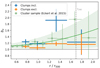 |
Fig. 6. Azimuthally averaged emissivity bias profiles before (blue) and after (orange) removal of the identified clumps. The overplotted green points and shaded region denote the measurements obtained for a sample of 31 clusters and their best-fit profile using a second order polynomial, as reported in Eckert et al. (2015). |
6. Spectral analysis
To study the thermodynamic structure of Abell 133, we performed a spectroscopic analysis with Suzaku data. We first divided the entire region into four azimuths (NW, NE, SW, and SE) and for each azimuth, we divided the observed region from 5′ to 30′ into five partial annuli, namely, 5′–8′, 8′–11′, 11′–15′, 15′–20′, 20′–30′. The first two annuli have a width of 3′ each, which are practically limited by the Suzaku PSF, while the outer annuli were set wider to improve the S/N. The spectra have been extracted from individual subdivided regions. Redistribution matrix files (RMFs) of the XIS were produced in the standard manner using xisrmfgen, and auxiliary response files (ARFs) by ray-tracing simulations using xissimarfgen (Ishisaki et al. 2007). For all the spectral analysis, we adopted the total column density NH = 1.74 × 1020 cm2 (Willingale et al. 2013)3. The abundance is fixed to 0.3 Solar beyond r500 (Werner et al. 2013; Urban et al. 2017) with the abundance table from Lodders et al. (2009) applied.
6.1. X-ray background modeling
Many previous studies of the ICM in the outskirts have only been based on Suzaku observations or with shallow Chandra exposure with the aim to exclude bright point sources. However, for Abell 133 and Abell 1795, we have deep multi-telescope coverage with Chandra and Suzaku, providing a unique opportunity to test how the thermodynamic measurements in the outskirts could be improved with a combination of low-background and high imaging resolution data. In order to investigate to what extent Chandra helps in reducing the systematic uncertainties related to the cosmic X-ray background (CXB) and how corrections for resolved clumping change the thermodynamic profiles, we carried out three rounds of spectral analysis, as introduced below.
In the first round of analysis, which is based on Suzaku data only (hereafter R1), we only removed Suzaku detected point sources (see Fig. B.1) and estimated the CXB normalization using the outermost spectra (i.e., extracted from 20′–30′), where the ICM temperature is expected to be lower than 2.5 keV. Since we also have to model the non–X-ray background (NXB; see Sect. 6.3), this procedure needs to follow several steps. We first performed a fit in the 0.7–12 keV band, modeling the observations and NXB spectra in parallel, with the index and normalization of the CXB component fixed to reasonable values (e.g., γ = 1.52 and norm = 1.0 × 10⁻³ photons keV−1 cm−2 s−1). During the fit, we allowed different overall norms between observations and NXB to account for the uncertainty of NXB. After obtaining the best-fit model, we set free both CXB parameters, freeze the NXB spectral model and fit only the 4–7 keV band where the CXB emission dominates. We found the best-fit indices for each annulus are statistically consistent with the adopted value, Γ = 1.52, therefore we fixed γ to minimize the free parameters in the subsequent analysis. The corresponding best-fit CXB norm is 1.05 × 10⁻³ photons keV−1 cm−2 s−1, which we have applied for the first round of analysis.
In the second round of analysis (R2), we further excluded the Chandra detected point sources with 2–8 keV flux above 5.67 × 10⁻¹⁵ erg cm−2 s−1, corresponding to 80% completeness, in order to suppress the CXB variation. The remaining unresolved CXB flux has been estimated using cxbtool (Mernier et al. 2015; de Plaa 2017), by integrating the derivative source luminosity function (dN/dS) fitted based on Chandra Deep Field South (CDFS; Lehmer et al. 2012) data. The integration gives an unresolved 2–8 keV flux of (8.77 ± 0.08) ×10−12 erg cm−2 s−1 deg−2. Since we use exclusion radii r ∼ 1′, which corresponds to the half-power diameter (HPD) of the Suzaku PSF, 50% of the total flux of the excluded point sources, namely, 2.02 × 10⁻¹² erg cm−2 s−1 deg−2, will have been scattered into our regions of interest. We therefore added this component to our model. When fitting the Suzaku spectra, we fixed the slope of the powerlaw model to Γ = 1.4 and normalization to 7.57 × 10⁻⁴ photons keV−1 cm−2 s−1.
To explore how clumps affect the thermodynamic profiles, we carried out the third round of spectral analysis (R3) by further excluding all the remaining clump candidates and utilizing the same CXB component as applied in the second round. We note that half of the 16 Chandra-selected clumps were not part of the Suzaku spectral analysis, either because they were outside of the field of view of the mosaic (BC1, BC2, C12, and C15), or because they are too close to point sources identified with Suzaku (C9, C11, C13, and C14). After masking Chandra point sources in R2, two more clumps (C6 and C10) were inevitably removed. Therefore we further removed 6 clumps (C3, C4, C5, C7, C8, and C16) in the third round of spectral analysis compared to R2.
6.2. X-ray foreground modeling
The X-ray foreground spectral model includes two thermal components modeling the Galactic halo (GH; Kuntz & Snowden 2000), and the local hot bubble (LHB; Sidher et al. 1996), respectively. To estimate the contribution of the GH and LHB, we obtained ROSAT All-sky Survey (RASS) data in an annulus between 1.5r200 and 2.5r200 around A133 with the ROSAT X-Ray Background Tool sxrbg4 (Sabol & Snowden 2019). In XSPEC, we fit the background spectrum in the 0.1–2 keV band with a tbabs*(apec+powerlaw)+apec model adopting AtomDB v3.09 and the abundance table from Lodders et al. (2009). We fixed the power-law parameters to the values reported by Kuntz & Snowden (2000; Γ = 1.46, and Y = 8.88 × 10⁻⁷ photons keV−1 cm−2 s−1 arcmin−2 at 1 keV) and fit them with χ2 statistics. More detailed information is given in Table 5.
Spectral fitting models and parameters.
Despite the fact that Abell 133 is located quite far from the Galactic Plane, where the ∼0.6 keV hot foreground (HF; Yoshino et al. 2009) originates, we checked the potential influence by adding this component. The χ2 statistics is not improved with this component included. Using ftest from the heasoft package, we calculate the F-statistic and its probability given the χ2 values and the corresponding degrees of freedom (d.o.f.) before and after adding this component. The obtained probability of 0.36 is not low enough to indicate the necessity of adding a new component.
6.3. Particle background modeling
We followed the procedures described in Zhu et al. (2021) to generate the particle background spectra and model them later in the spectral analysis. In brief, we created the NXB spectrum of each XIS sensor using xisnxbgen, which extracts spectra from the integrated night-Earth data collected during the period of ±150 days from the target observation. Based on Fig. 1 of Tawa et al. (2008), we modeled the NXB spectra of the FI CCDs (XIS 0 and XIS 3) with a power-law for the continuum and nine Gaussian components for the instrumental lines. For the BI CCD (XIS1), we added another broad Gaussian model to account for the continuum bump above 7 keV. More details can be found in Sect. 2.5 and Appendix D of Zhu et al. (2021).
7. Thermodynamic profiles
7.1. Suzaku projected profiles
The projected temperature profiles of four different azimuths obtained from the analysis described in Sect. 6 are shown in the left panel of Fig. 7. The scatter of the measurements along different azimuths indicates the inhomogeneity and asymmetry of the ICM. There is no signal measured between 20′–30′ towards the southeast (SE). The measured temperatures in the northwest (NW) and southeast (SE) are overall lower compared to the other two azimuths, which might be explained by the orientation of the major axis of Abell 133. In the right panel of Fig. 7, we present the azimuthally averaged projected temperature profiles and we compare the results obtained with the several different analysis rounds introduced in Sect. 6.1. The profiles are generally in good agreement for all rounds of analysis.
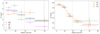 |
Fig. 7. Projected temperature profiles. Left: First round results (R1), using only the Suzaku data. The grey shaded regions denote the azimuthally-averaged temperature measurements. The dotted and dashed lines show the radius of r500 and r200 respectively. Right: Comparison between different rounds of azimuthally averaged measurements. All three rounds of spectra were extracted from the same annuli but shifted by 0.5′ in this plot for illustration purpose. The abundance is fixed to 0.3 beyond r500 (Werner et al. 2013; Urban et al. 2017). |
7.2. Deprojected spectral results
To obtain the deprojected properties, we applied the XSPEC model projct while assuming spherical symmetry. With projct, the ICM in each annulus is modeled as the superposition of the ICM from a shell corresponding to that annulus, with the emission projected on to that annulus from the shells exterior to it. The emission from each shell is described by an absorbed apec model. The deprojected densities are derived from the apec normalizations for each annulus obtained during the spectral fitting, using the volumes of each shell and assuming the plasma is fully ionized with ne:nH = 1.2:1. We generated a background spectrum based on the best-fit NXB model using fakeit, setting the exposure the same as the original NXB spectrum produced by xisnxbgen, to ensure the statistical uncertainties of the NXB spectrum have been properly propagated while the applied background spectrum is smooth and free from outliers in the initial background data. Based on the resulting measurements of deprojected temperatures and electron density, we further derived the deprojected pressure (P = nekT) and entropy ( ). In Fig. 8, we compare the azimuthally averaged entropy and pressure profiles with their reference models described below.
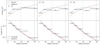 |
Fig. 8. Azimuthally averaged profiles of the ICM properties. Top: Entropy profile. The orange line shows the entropy model calculated according to Pratt et al. (2010). The blue line indicates the best-fit entropy profile by Walker et al. (2012). Bottom: Pressure profile with overplotted models by Arnaud et al. (2010) (purple line) and Planck Collaboration Int. V (2013) (olive line). The dotted and dashed vertical lines show the radius of r500 and r200, respectively. |
7.2.1. Entropy profile
In a cluster formed by gravitational collapse without additional heating or cooling, the entropy is expected to follow a power-law:

where K500 = 106 keV cm2(M500/1014 M⊙)2/3(1/fb)2/3E(z)−2/3 (Voit et al. 2005; Pratt et al. 2010)5. We adopted fb = 0.15, r500 = 14.6′ and M500 = 3.2 × 10¹⁴ M⊙ (Vikhlinin et al. 2006) in calculating K500.
As shown in Fig. 8, beyond ∼0.7r200 we observed a flattening of the entropy profile with respect to this expected power-law for all three rounds of analysis. We overplotted the model introduced by Walker et al. (2012), who proposed that the entropy profile outside of 0.2r200 can be fitted with an analytical function:
![$$ \begin{aligned} K/K (0.3r_{200}) = A (r/r_{200})^{1.1}\,\mathrm{exp}[ - (r/Br_{200})^{2} ], \end{aligned} $$](/articles/aa/full_html/2023/10/aa47191-23/aa47191-23-eq23.gif)
with (A, B) =  . The entropy profiles of all three rounds (in particular, the outermost measurement) do indeed achieve a better match with this second model.
7.2.2. Pressure profile
We utilized the generalized NFW pressure profile proposed by Nagai et al. (2007) as a reference model, which takes the following form:
![$$ \begin{aligned} \frac{P(r) }{ P_{500} } = \frac{ P_{0} }{(c_{500}x)^{\gamma } [1+(c_{500}x)^{\alpha }]^{(\beta -\gamma )/\alpha } }, \end{aligned} $$](/articles/aa/full_html/2023/10/aa47191-23/aa47191-23-eq25.gif)
where x = r/R500, P0 is the normalization, c500 is the concentration parameter defined at r500, and the indices α, β, and γ are the profile slopes in the intermediate, outer, and central regions. The characteristic pressure, P500, scales with the cluster mass:
![$$ \begin{aligned} P_{500} = 1.65\times 10^{-3} E(z)^{8/3}\times \left[ \frac{M_{500}}{3\times 10^{14}\,h_{70}^{-1}\,{M}_{\odot }} \right] ^{2/3}\,h_{70}^{2}\,\mathrm{keV}\,\mathrm{cm}^{-3}. \end{aligned} $$](/articles/aa/full_html/2023/10/aa47191-23/aa47191-23-eq26.gif)
Arnaud et al. (2010) gave the best-fit parameters, (P0, c500, α, β, γ)A = (8.403, 1.177, 1.0510, 5.4905, 0.3081) by fitting 33 nearby (z < 0.2) clusters out to 0.6r200. By analyzing 62 Planck clusters between 0.02r500 < r < 3r500, Planck Collaboration Int. V (2013) obtained another set of parameters as (P0, c500, α, β, γ)P = (6.41, 1.81, 1.33, 4.13, 0.31). As shown in the lower panel of Fig. 8, our measurements show a reasonable agreement with the Planck measurements, although the outermost data point appears marginally higher.
8. Discussion
To understand how the addition of complementary high-spatial resolution Chandra data improves our understanding of the ICM measurements, we carefully compared the results between Suzaku-based (R1) and Chandra-involved (R2 and R3) analysis. As shown in the right panel of Fig. 7, the projected temperatures measured in different rounds are roughly consistent within statistical uncertainties. The deprojected profiles show a difference in the 15′–20′ annulus between R1 and R2 results. However, this is simply due to the fact that for the Suzaku only analysis, we were forced to couple the ICM temperature of the 15′–20′ annulus to that of the 10′–15′ annulus when fitting with projct. With Chandra-selected point sources removed, R2 and R3 have more precise constraints on the CXB level and the cosmic variance has been suppressed; thus, the deprojection was more stable and this coupling of temperatures between neighboring annuli was no longer needed.
8.1. Systematic uncertainties
Spatial variations in the foreground emission and cosmic variance can introduce systematic uncertainties in the measured thermodynamic profiles. To estimate the variation of GH, we extracted RASS spectra of circles with radius of 1 degree in four different azimuths outside 1.5r200. We then calculated the variance in the best-fit normalization of GH. The obtained 27% systematic uncertainty for GH is then taken into account. The expected cosmic variance due to unresolved point sources over a solid angle Ω is
where Ω is the solid angle (Bautz et al. 2009). We substituted the derivative source function (dN/dS) given in Lehmer et al. (2012) and adopted a flux cut of Sexcl = 5.67 × 10⁻¹⁵ erg cm−2 s−1 (see Sect. 6.1) for R3. We found the relative cosmic variance σB/B in the outermost annulus decreases from 6% in R1 to 3% in R3.
In Fig. 9, we demonstrate the impact of systematic uncertainties on the azimuthally-averaged temperatures for R1 and R3. For the Suzaku-only analysis shown in the upper panel, it is noteworthy that while systematic errors are comparable with the statistical errors for measurements within r500, they become increasingly larger in the outskirts especially approaching r200. It also shows that outside 1.4r500 thermodynamic measurement results become extremely sensitive to the cosmic variance, while for the inner regions, they are much more robust. For the outermost bin, systematic uncertainties from the GH emission have also increased likely due to model degeneracies causing the best fit ICM component to compensate for a combination of GH and CXB residuals. The measurements roughly match with the expectation from hydrodynamic cosmological simulations (Burns et al. 2010), taking into account the large systematic error on the outermost data point. Through a comparison of the upper (R1) and lower (R3) panels of Fig. 9, we show that the systematic uncertainties have been significantly reduced after the removal of more point sources benefiting from the Chandra observations.
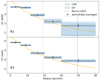 |
Fig. 9. Suzaku temperature profile of Abell 133. Systematic uncertainties from best-fit GH model and CXB estimation are denoted by blue slash region and shaded region respectively. The upper and lower panels show the differences before and after removal of point sources (S2 − 8 > 5.67 × 10⁻¹⁵ erg cm−2 s−1) and clumps. The orange solid line represents the expectation from hydrodynamic cosmological simulations (Burns et al. 2010). |
8.2. Clumping correction
In the lower panels of Fig. 10, we compare the density profiles of different rounds. We applied power-law modeling for the density profiles of the outskirts of Abell 133, ne = n0r−δ.
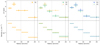 |
Fig. 10. Deprojected temperature and density profiles. Left:Suzaku only measurements (R1) denoted with orange data points. Middle: Measurements using the Chandra point source list (R2) shown as green data points, with R1 results overplotted. Right: The comparison between profiles before (R2) and after (R3) the removal of Chandra-detected clumps. |
We report a relatively flat azimuthally averaged density profile of R2, falling off with radius with an index of δ = 1.60 ± 0.06 outside 0.6 Mpc (r > 0.4r200). This is in agreement with the slope reported by Urban et al. (2014) for the Perseus Cluster in the same scaled radial range. After removing the resolved clumps, the best-fit density slope of R3 outside 0.4r200 remains the same as R2. However, as shown in Fig. 8, even after the correction of resolved clumps, the entropy profile approaching the outskirts still flattens, significantly deviating from the power law model (Pratt et al. 2010).
By integrating Eq. (1) with Eq. (3), while utilizing the Planck Collaboration Int. V (2013) parameters for Eq. (3), we can solve for the expected ne and kT profiles. In Fig. 11, we compare the measured density and temperature with these baseline expectations. We found the ne measured from R3, which has been best corrected for the clumping, still deviates from the baseline beyond r500. The ratio between the measured and predicted ne progressively increases towards the outskirts, ultimately reaching a value of 2.0 in the outermost bin.
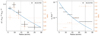 |
Fig. 11. Self-similarly scaled temperature and density profiles of Abell 133. The dotted and dashed lines show the radius of r500 and r200, respectively. P500 and K500 are defined in Sect. 7. The reference model derived from the referenced pressure and entropy profiles is denoted with a blue solid curve. The orange dashed points represent the ratio between the measurements and the reference models, for better comparison. |
8.3. Non-thermal pressure or electron-ion non-equilibrium
In addition to the remaining unresolved clumping bias, there is also a temperature bias in the outskirts; namely, the measurements appear lower than the expected values. Here, we discuss two explanations for this discrepancy.
Besides clumping, other ways to explain the entropy deficit seen in the cluster outskirts involve scenarios wherein a sizeable fraction of the gravitational energy due to infall is not thermalized immediately. For example, Ghirardini et al. (2018) found that the entropy profile of Abell 2319 measured from the joint analysis of the X-ray and Sunyaev-Zel’dovich (SZ) signals still shows a deficit near r200, even after correcting for gas clumping. The authors attribute this to a level of non-thermal pressure due to gas motions and turbulence, amounting to 40% of the thermal pressure near the virial radius. Similar physics could be responsible for the entropy (and temperature) deficit in the outskirts of A133, especially given its prominent radio relics indicating recent merging activity. Quantitative estimation of the proportion of non-thermal pressure however requires hydrostatic mass modeling, which is beyond the scope of this work.
Alternatively, the relatively low kT measured in the outskirts could result from non-equilibrium. When a plasma of electrons and ions travels through a shock, most of the kinetic energy goes into heating the heavier ions, causing Ti ≫ Te. However, with CCD spectroscopy, we can only measure the electron temperature, which may represent an underestimation of the overall gas temperature. After the shock, electrons and ions slowly equilibrate over a typical timescale, which is given by
(Spitzer 1962). We substitute the Te and ni of the outermost annulus from R3 results into this equation and obtain a timescale of 3.8 × 10⁸ years. The past accretion event could be more recent compared to this timescale, causing the measured temperature to be lower than expectations.
9. Conclusion
In this work, we explored the Suzaku and Chandra data of Abell 133, one of the galaxy clusters with the best X-ray coverage of its outskirts region. After removing point sources, we identified 16 clump candidates with at least 2σ significance from the Chandra image. Combining the cluster catalogue from the DESI Legacy Imaging Surveys and the r-band image taken with CFHT, we discussed the origin of individual clump candidates, finding that Chandra-selected clumps are mainly background clusters or galaxies, instead of genuine inhomogeneity.
We performed three rounds of Suzaku spectral analysis and derived the thermodynamic profiles to large radii of the Abell 133. We further compared thermodynamic profiles after the correction for resolved clumps by removing them from spectral extraction. In general, none of the thermodynamic profiles are heavily affected by the corrections applied. For the case of Abell 133, even after the correction for the clumping resolved by very deep Chandra data, we still see an entropy deficit and a density excess compared to the expectations. This suggests that the effect of unresolved clumping is potentially important and must still be taken into account, even when analyzing very sensitive, high spatial resolution data. Aside from the density bias, we also report a mild underestimation of the temperature at large radii. It is therefore possible that other physical mechanisms (e.g., non-thermal pressure or non-equilibrium electrons in the ICM) in the outskirts may play an additional role.
Online calculator for Galactic column density: https://www.swift.ac.uk/analysis/nhtot/index.php
Acknowledgments
We would like to thank Henk Hoekstra for access to CFHT data of Abell 133 and Konstantinos Migkas for useful discussion about Suzaku cosmic X-ray background estimation. We also thank the anonymous referee for useful suggestions that improved this paper. ZZ, AS are supported by the Netherlands Organisation for Scientific Research (NWO). The Space Research Organization of the Netherlands (SRON) is supported financially by NWO. OEK and NW are supported by the GAČR EXPRO grant No. 21-13491X “Exploring the Hot Universe and Understanding Cosmic Feedback”. This research is mainly based on observations obtained from the Suzaku satellite, a collaborative mission between the space agencies of Japan (JAXA) and the USA (NASA). This research has also made use of data obtained from the Chandra Data Archive and software provided by the Chandra X-ray Center (CXC) in the application package CIAO.
References
- Arnaud, M., Pratt, G. W., Piffaretti, R., et al. 2010, A&A, 517, A92 [CrossRef] [EDP Sciences] [Google Scholar]
- Avestruz, C., Nagai, D., Lau, E. T., & Nelson, K. 2015, ApJ, 808, 176 [CrossRef] [Google Scholar]
- Bautz, M. W., Miller, E. D., Sanders, J. S., et al. 2009, PASJ, 61, 1117 [NASA ADS] [Google Scholar]
- Burns, J. O., Skillman, S. W., & O’Shea, B. W. 2010, ApJ, 721, 1105 [NASA ADS] [CrossRef] [Google Scholar]
- Connor, T., Kelson, D. D., Mulchaey, J., et al. 2018, ApJ, 867, 25 [Google Scholar]
- de Plaa, J. 2017, https://doi.org/10.5281/zenodo.2575495 [Google Scholar]
- Eckert, D., Molendi, S., & Paltani, S. 2011, A&A, 526, A79 [NASA ADS] [CrossRef] [EDP Sciences] [Google Scholar]
- Eckert, D., Roncarelli, M., Ettori, S., et al. 2015, MNRAS, 447, 2198 [Google Scholar]
- Fujita, Y., Sarazin, C. L., Kempner, J. C., et al. 2002, ApJ, 575, 764 [CrossRef] [Google Scholar]
- Ghirardini, V., Ettori, S., Eckert, D., et al. 2018, A&A, 614, A7 [NASA ADS] [CrossRef] [EDP Sciences] [Google Scholar]
- Graham, M. L., Sand, D. J., Bildfell, C. J., et al. 2012, ApJ, 753, 68 [CrossRef] [Google Scholar]
- Hoshino, A., Henry, J. P., Sato, K., et al. 2010, PASJ, 62, 371 [CrossRef] [Google Scholar]
- Ishisaki, Y., Maeda, Y., Fujimoto, R., et al. 2007, PASJ, 59, 113 [NASA ADS] [Google Scholar]
- Kovács, O. E., Zhu, Z., Werner, N., Simionescu, A., & Bogdán, Á. 2023, A&A, 678, A91 [NASA ADS] [CrossRef] [EDP Sciences] [Google Scholar]
- Kuntz, K. D., & Snowden, S. L. 2000, ApJ, 543, 195 [Google Scholar]
- Lehmer, B. D., Xue, Y. Q., Brandt, W. N., et al. 2012, ApJ, 752, 46 [NASA ADS] [CrossRef] [Google Scholar]
- Lodders, K., Palme, H., & Gail, H. P. 2009, Landolt Börnstein, 4B, 712 [Google Scholar]
- Mernier, F., de Plaa, J., Lovisari, L., et al. 2015, A&A, 575, A37 [NASA ADS] [CrossRef] [EDP Sciences] [Google Scholar]
- Mirakhor, M. S., & Walker, S. A. 2021, MNRAS, 506, 139 [NASA ADS] [CrossRef] [Google Scholar]
- Mohr, J. J., Mathiesen, B., & Evrard, A. E. 1999, ApJ, 517, 627 [Google Scholar]
- Morandi, A., & Cui, W. 2014, MNRAS, 437, 1909 [Google Scholar]
- Nagai, D., & Lau, E. T. 2011, ApJ, 731, L10 [NASA ADS] [CrossRef] [Google Scholar]
- Nagai, D., Kravtsov, A. V., & Vikhlinin, A. 2007, ApJ, 668, 1 [Google Scholar]
- Nelson, K., Lau, E. T., & Nagai, D. 2014, ApJ, 792, 25 [NASA ADS] [CrossRef] [Google Scholar]
- Ota, N., & Yoshida, H. 2016, PASJ, 68, S19 [NASA ADS] [CrossRef] [Google Scholar]
- Planck Collaboration Int. V. 2013, A&A, 550, A131 [NASA ADS] [CrossRef] [EDP Sciences] [Google Scholar]
- Pratt, G. W., Arnaud, M., Piffaretti, R., et al. 2010, A&A, 511, A85 [NASA ADS] [CrossRef] [EDP Sciences] [Google Scholar]
- Randall, S. W., Clarke, T. E., Nulsen, P. E. J., et al. 2010, ApJ, 722, 825 [NASA ADS] [CrossRef] [Google Scholar]
- Sabol, E. J., & Snowden, S. L. 2019, sxrbg: ROSAT X-Ray Background Tool, Astrophysics Source Code Library, [record ascl:1904.001] [Google Scholar]
- Sand, D. J., Graham, M. L., Bildfell, C., et al. 2012, ApJ, 746, 163 [NASA ADS] [CrossRef] [Google Scholar]
- Sanders, J. S. 2006, MNRAS, 371, 829 [Google Scholar]
- Shin, J., Plotkin, R. M., Woo, J.-H., Gallo, E., & Mulchaey, J. S. 2018, ApJS, 238, 23 [NASA ADS] [CrossRef] [Google Scholar]
- Sidher, S. D., Sumner, T. J., Quenby, J. J., & Gambhir, M. 1996, A&A, 305, 308 [NASA ADS] [Google Scholar]
- Simionescu, A., Allen, S. W., Mantz, A., et al. 2011, Science, 331, 1576 [Google Scholar]
- Simionescu, A., Werner, N., Urban, O., et al. 2013, ApJ, 775, 4 [Google Scholar]
- Simionescu, A., Werner, N., Mantz, A., Allen, S. W., & Urban, O. 2017, MNRAS, 469, 1476 [Google Scholar]
- Spitzer, L. 1962, Physics of Fully Ionized Gases (New York: Interscience) [Google Scholar]
- Struble, M. F., & Rood, H. J. 1999, ApJS, 125, 35 [Google Scholar]
- Tawa, N., Hayashida, K., Nagai, M., et al. 2008, PASJ, 60, S11 [NASA ADS] [Google Scholar]
- Tchernin, C., Eckert, D., Ettori, S., et al. 2016, A&A, 595, A42 [NASA ADS] [CrossRef] [EDP Sciences] [Google Scholar]
- Urban, O., Simionescu, A., Werner, N., et al. 2014, MNRAS, 437, 3939 [Google Scholar]
- Urban, O., Werner, N., Allen, S. W., Simionescu, A., & Mantz, A. 2017, MNRAS, 470, 4583 [Google Scholar]
- Varela, J., D’Onofrio, M., Marmo, C., et al. 2009, A&A, 497, 667 [NASA ADS] [CrossRef] [EDP Sciences] [Google Scholar]
- Vikhlinin, A. 2013, in AAS/High Energy Astrophysics Division, AAS/High Energy Astrophysics Division, 13, 401.01 [NASA ADS] [Google Scholar]
- Vikhlinin, A., Markevitch, M., Murray, S. S., et al. 2005, ApJ, 628, 655 [Google Scholar]
- Vikhlinin, A., Kravtsov, A., Forman, W., et al. 2006, ApJ, 640, 691 [Google Scholar]
- Voit, G. M., Kay, S. T., & Bryan, G. L. 2005, MNRAS, 364, 909 [NASA ADS] [CrossRef] [Google Scholar]
- Walker, S. A., Fabian, A. C., Sanders, J. S., & George, M. R. 2012, MNRAS, 427, L45 [Google Scholar]
- Walker, S. A., Fabian, A. C., Sanders, J. S., Simionescu, A., & Tawara, Y. 2013, MNRAS, 432, 554 [Google Scholar]
- Walker, S., Simionescu, A., Nagai, D., et al. 2019, Space Sci. Rev., 215, 7 [Google Scholar]
- Wang, S., Liu, J., Qiu, Y., et al. 2016, ApJS, 224, 40 [Google Scholar]
- Werner, N., Urban, O., Simionescu, A., & Allen, S. W. 2013, Nature, 502, 656 [Google Scholar]
- Willingale, R., Starling, R. L. C., Beardmore, A. P., Tanvir, N. R., & O’Brien, P. T. 2013, MNRAS, 431, 394 [Google Scholar]
- Yoshino, T., Mitsuda, K., Yamasaki, N. Y., et al. 2009, PASJ, 61, 805 [NASA ADS] [Google Scholar]
- Zhu, Z., Simionescu, A., Akamatsu, H., et al. 2021, A&A, 652, A147 [NASA ADS] [CrossRef] [EDP Sciences] [Google Scholar]
- Zhuravleva, I., Churazov, E., Kravtsov, A., et al. 2013, MNRAS, 428, 3274 [NASA ADS] [CrossRef] [Google Scholar]
- Zou, H., Gao, J., Xu, X., et al. 2021, ApJS, 253, 56 [NASA ADS] [CrossRef] [Google Scholar]
Appendix A: Solar proton flux variation during Suzaku observations
We checked for potential contamination from solar wind charge exchange (SWCX). In Fig.A.1 we plotted the solar proton flux measured by WIND spacecraft’s solar wind experiment instrument during 2010 Jun 5-12 and 2013 Dec 5-9 and 19-23, which cover the periods of all 8 Suzaku observations used in our analysis. Fig.A.1 shows that the proton flux is below 4 × 108 cm−2 s−1 for observation N, W, F1, F2, F3, and F4, therefore, it will not produce significant contamination Yoshino et al. (2009). For observation S and E, we have checked the count rate of 0.7–1.2 keV where SWCX contributes the most, and this value remains unchanged within the uncertainty range. Therefore, despite the proton flux increases, these two observations appear to be free from SWCX contamination.
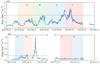 |
Fig. A.1. Solar proton flux measured by the WIND spacecraft’s solar wind experiment instrument. The shaded regions denote the time coverage of Suzaku observations, corrected for the particle travel time to the earth. |
Appendix B: Suzaku selected point sources
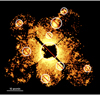 |
Fig. B.1. Exposure- and vignetting-corrected 0.7–7 keV Suzaku image of Abell 133 with the point sources that have been excluded in the Suzaku-only analysis (R1) overplotted. |
All Tables
All Figures
|
Fig. 1. Exposure- and vignetting-corrected 0.7–7 keV Suzaku image of Abell 133. The 90-degree white annuli show extraction regions applied in the spectral analysis. |
| In the text | |
|
Fig. 2. Contour binned image of the inner 30′ of Abell 133 in the 0.5–3 keV energy band. The point sources detected by wavdetect have been removed. Each bin has a S/N ≥ 3, and an average photon flux as indicated by the color bar in units of photon cm−2 s−1 pixel−1. Here, 1 pixel corresponds to 0.98″. |
| In the text | |
|
Fig. 3. 0.5–3 keV background-subtracted azimuthally averaged surface brightness profile of the outskirts of Abell 133 obtained from Chandra (black) and Suzaku (grey) data with the corresponding best-fit power-law models overplotted. The Suzaku sky background level is relatively higher compared to Chandra, which reflects the excess emission from Chandra-selected point sources whose PSF is broader than the source extraction region. |
| In the text | |
|
Fig. 4. 0.5–3 keV surface brightness distribution of Abell 133 outskirts obtained in 4 annuli, mapping from 10.2′ to 30.0′ as listed in Table 3. The histogram in grey shows the contribution from the large, bright diffuse features in the southeast, which have been excluded from further analysis. The solid orange line marks the 2σ outlier threshold. |
| In the text | |
|
Fig. 5. 0.5–3 keV cut-out images for clump candidates (white regions). Left: Each Chandra image has a size of 200″ × 200″ (0.2 Mpc × 0.2 Mpc) and is smoothed with a Gaussian function with a kernel of 6 pixels. Filled black ellipses represent excluded wavdetect sources. The orange dashed circles mark the r500 radius of background clusters (Zou et al. 2021). Right:r-band CFHT image showing the same field of view. |
| In the text | |
|
Fig. 5. continued. |
| In the text | |
|
Fig. 6. Azimuthally averaged emissivity bias profiles before (blue) and after (orange) removal of the identified clumps. The overplotted green points and shaded region denote the measurements obtained for a sample of 31 clusters and their best-fit profile using a second order polynomial, as reported in Eckert et al. (2015). |
| In the text | |
|
Fig. 7. Projected temperature profiles. Left: First round results (R1), using only the Suzaku data. The grey shaded regions denote the azimuthally-averaged temperature measurements. The dotted and dashed lines show the radius of r500 and r200 respectively. Right: Comparison between different rounds of azimuthally averaged measurements. All three rounds of spectra were extracted from the same annuli but shifted by 0.5′ in this plot for illustration purpose. The abundance is fixed to 0.3 beyond r500 (Werner et al. 2013; Urban et al. 2017). |
| In the text | |
|
Fig. 8. Azimuthally averaged profiles of the ICM properties. Top: Entropy profile. The orange line shows the entropy model calculated according to Pratt et al. (2010). The blue line indicates the best-fit entropy profile by Walker et al. (2012). Bottom: Pressure profile with overplotted models by Arnaud et al. (2010) (purple line) and Planck Collaboration Int. V (2013) (olive line). The dotted and dashed vertical lines show the radius of r500 and r200, respectively. |
| In the text | |
|
Fig. 9. Suzaku temperature profile of Abell 133. Systematic uncertainties from best-fit GH model and CXB estimation are denoted by blue slash region and shaded region respectively. The upper and lower panels show the differences before and after removal of point sources (S2 − 8 > 5.67 × 10⁻¹⁵ erg cm−2 s−1) and clumps. The orange solid line represents the expectation from hydrodynamic cosmological simulations (Burns et al. 2010). |
| In the text | |
|
Fig. 10. Deprojected temperature and density profiles. Left:Suzaku only measurements (R1) denoted with orange data points. Middle: Measurements using the Chandra point source list (R2) shown as green data points, with R1 results overplotted. Right: The comparison between profiles before (R2) and after (R3) the removal of Chandra-detected clumps. |
| In the text | |
|
Fig. 11. Self-similarly scaled temperature and density profiles of Abell 133. The dotted and dashed lines show the radius of r500 and r200, respectively. P500 and K500 are defined in Sect. 7. The reference model derived from the referenced pressure and entropy profiles is denoted with a blue solid curve. The orange dashed points represent the ratio between the measurements and the reference models, for better comparison. |
| In the text | |
|
Fig. A.1. Solar proton flux measured by the WIND spacecraft’s solar wind experiment instrument. The shaded regions denote the time coverage of Suzaku observations, corrected for the particle travel time to the earth. |
| In the text | |
|
Fig. B.1. Exposure- and vignetting-corrected 0.7–7 keV Suzaku image of Abell 133 with the point sources that have been excluded in the Suzaku-only analysis (R1) overplotted. |
| In the text | |
Current usage metrics show cumulative count of Article Views (full-text article views including HTML views, PDF and ePub downloads, according to the available data) and Abstracts Views on Vision4Press platform.
Data correspond to usage on the plateform after 2015. The current usage metrics is available 48-96 hours after online publication and is updated daily on week days.
Initial download of the metrics may take a while.