| Issue |
A&A
Volume 684, April 2024
|
|
|---|---|---|
| Article Number | A4 | |
| Number of page(s) | 114 | |
| Section | Interstellar and circumstellar matter | |
| DOI | https://doi.org/10.1051/0004-6361/202346264 | |
| Published online | 29 March 2024 | |
Charting circumstellar chemistry of carbon-rich asymptotic giant branch stars
I. ALMA 3 mm spectral surveys★
1
Department of Space, Earth and Environment, Chalmers University of Technology,
412 96
Gothenburg, Sweden
e-mail: ramlal.unnikrishnan@chalmers.se
2
Department of Space, Earth and Environment, Chalmers University of Technology, Onsala Space Observatory (OSO),
439 92
Onsala, Sweden
3
Joint ALMA Observatory (JAO),
Alonso de Cordova 3107, Vitacura 763-0355, Casilla
19001,
Santiago, Chile
4
European Southern Observatory (ESO),
Alonso de Cordova 3107, Vitacura
763-0355,
Santiago, Chile
5
NASA Goddard Space Flight Center,
8800 Greenbelt Road,
Greenbelt, MD
20771, USA
6
Solar System Exploration Division, NASA Goddard Space Flight Center,
8800 Greenbelt Road,
Greenbelt, MD
20771, USA
7
Department of Physics, Catholic University of America,
Washington, DC
20064, USA
8
Astrophysics Research Centre, School of Mathematics and Physics, Queen’s University Belfast,
University Road,
Belfast
BT7 1NN, UK
9
Gemini Observatory / NSF’s NOIRLab,
670 N. A’ohoku Place, Hilo,
Hawai’i
96720, USA
10
East Asian Observatory / James Clerk Maxwell Telescope,
660 N. A’ohoku Place,
Hilo, HI
96720, USA
Received:
28
February
2023
Accepted:
4
December
2023
Context. Asymptotic giant branch (AGB) stars are major contributors to the chemical enrichment of the interstellar medium through nucleosynthesis and extensive mass loss. Direct measures of both processes can be obtained by studying their circumstellar envelopes in molecular line emission. Most of our current knowledge of circumstellar chemistry, in particular in a C-rich environment, is based on observations of the carbon star IRC +10216.
Aims. We aim to obtain a more generalised understanding of the chemistry in C-rich AGB circumstellar envelopes by studying a sample of three carbon stars, IRAS 15194–5115, IRAS 15082–4808, and IRAS 07454–7112, and to observationally test the archetypal status often attributed to IRC +10216.
Methods. We performed spatially resolved, unbiased spectral surveys in ALMA Band 3 (85–116 GHz). We estimated the sizes of the molecular emitting regions using azimuthally averaged radial profiles of the line brightness distributions. We derived abundance estimates, using a population diagram analysis for molecules with multiple detected lines, and using single-line analytical calculations for the others.
Results. We identify a total of 132 rotational transitions from 49 molecular species. There are two main morphologies of the brightness distributions: centrally peaked (CS, SiO, SiS, HCN) and shell-like (CN, HNC, C2H, C3H, C4H, C3N, HC5N, c-C3H2). The brightness distributions of HC3N and SiC2 have both a central and a shell component. The qualitative behaviour of the brightness distributions of all detected molecules, in particular their relative locations with respect to the central star, is the same for all three stars, and consistent with those observed towards IRC +10216. Of the shell distributions, the cyanopolyynes peak at slightly smaller radii than the hydrocarbons, and CN and HNC show the most extended emission. The emitting regions for each species are the smallest for IRAS 07454–7112, consistent with this object having the lowest circumstellar density within our sample. We find that, within the uncertainties of the analysis, the three stars present similar abundances for most species, and also compared to IRC +10216. We find, tentatively, that SiO is more abundant in our three stars compared to IRC+10216, and that the hydrocarbons are under-abundant in IRAS 07454–7112 compared to the other stars and IRC +10216. Our estimated 12C/13C ratios match well the literature values for the three sources and our estimated silicon and sulphur isotopic ratios are very similar across the three stars and IRC +10216.
Conclusions. The observed circumstellar chemistry appears very similar across our sample and compared to that of IRC +10216, both in terms of the relative location of the emitting regions and molecular abundances. This implies that, to a first approximation, the chemical models tailored to IRC +10216 are, at least, able to reproduce the observed chemistry in C-rich envelopes across roughly an order of magnitude in wind density.
Key words: astrochemistry / stars: AGB and post-AGB / circumstellar matter / stars: mass-loss / stars: winds, outflows / submillimeter: stars
The re-reduced ALMA cubes, line spectra, and continuum maps are available at the CDS via anonymous ftp to cdsarc.cds.unistra.fr (138.79.128.5) or via https://cdsarc.cds.unistra.fr/viz-bin/cat/J/A+A/684/A4
© The Authors 2024
 Open Access article, published by EDP Sciences, under the terms of the Creative Commons Attribution License (https://creativecommons.org/licenses/by/4.0), which permits unrestricted use, distribution, and reproduction in any medium, provided the original work is properly cited.
This article is published in open access under the Subscribe to Open model. Subscribe to A&A to support open access publication.
1 Introduction
Stars of low to intermediate zero-age main sequence mass (~0.8 M⊙ < M < 8 M⊙) populate the asymptotic giant branch (AGB) during their late evolution, after the end of helium fusion in their cores. In this phase, stars are characterised by an inert carbon-oxygen core surrounded by shells of helium and hydrogen. Contraction of the core causes the outer layers of the star to expand, resulting in cool, luminous giants (Teff ≲ 3000 K, L* ~ 103–104L⊙, R* ~ 100 R⊙; Herwig 2005). Microscopic dust grains (with radius a in the range 0.1 μm ≤ a ≤ 0.5 μm, e.g. Groenewegen 1997; Höfner 2008; Yasuda & Kozasa 2012) formed in the cool, dense upper stellar atmosphere are levitated by pulsations, accelerated by radiation pressure, and push gas radially outwards through dust-gas momentum exchange (Höfner 2015). This causes extensive mass loss from the stellar surface. AGB mass-loss rates (hereafter MLRs) range from 10−8 to 10−4 M⊙ yr−1, dominating the evolution on the AGB (e.g. Höfner & Olofsson 2018). The winds of AGB stars are major sources of gas and dust feedback into the interstellar medium (ISM, e.g. Matsuura et al. 2009; Tielens 2005).
The mass loss creates an expanding envelope of chemically rich material around the star, called the circumstellar envelope (CSE). The radial density distribution of material in the CSE is a tracer of the temporal variations in the mass loss. The elemental compositions of gas and dust in the CSE reflect the composition of the atmosphere of the star at the time of the ejection of the circumstellar material.
Based on their atmospheric carbon-to-oxygen elemental abundance ratio, AGB stars are classified into two main groups: C-type (C/O > 1) and M-type (C/O < 1). AGB stars in the mass range 1.5–4 M⊙ (at solar composition) evolve into C-type stars in the absence of hot-bottom burning (Lattanzio et al. 1997), as the carbon produced in the helium-burning layer is brought up to the surface by convection (e.g. Di Criscienzo et al. 2016) during the third dredge-up (Herwig 2005). The excess of carbon over oxygen for C-type stars allows a wide range of C-bearing species to form in their CSEs, including long carbon chains and possibly also PAHs (e.g. Cherchneff et al. 1992; Allain et al. 1997), as well as carbonaceous dust (e.g. Kraemer et al. 2019; Sloan et al. 1998; Zijlstra et al. 2006). With 96 molecular species detected in carbon star CSEs so far, compared to only around 34 species found in oxygen-rich circumstellar environments, the CSEs of C-type stars are generally richer in chemistry than those of their M-type counterparts (Agúndez 2022; McGuire 2022; Cernicharo et al. 2023a,b).
The advent of high-angular-resolution mm/sub-mm interferometers like the Atacama Large Millimeter/submillimeter Array (ALMA) has made it possible to explore the chemical complexity of AGB CSEs in unmatched detail. However, notwithstanding these significant advances in instrumentation, much of our current knowledge of AGB circumstellar chemistry is still based on observational results and modelling focused on a single object, the C-type IRC +10216 (CW Leonis), owing primarily to its proximity (120–190 pc), high MLR (Ṁ = 2–4 × 10⁻⁵ M⊙ yr−1), and molecular richness (e.g. Andriantsaralaza et al. 2022; Agúndez et al. 2017; He et al. 2008; Cernicharo et al. 2000; Cordiner & Millar 2009; Groenewegen et al. 2012; Guélin et al. 2018; Pardo et al. 2022; Patel et al. 2011; Tenenbaum et al. 2010; Velilla-Prieto et al. 2019; Van de Sande et al. 2019).
Studies of the molecular chemistry in the CSE of IRC +10216, from single-dish spectral surveys (e.g. Cernicharo et al. 2000; Agúndez et al. 2012) to interferometric maps (e.g. Patel et al. 2011; Velilla Prieto et al. 2015a; Agúndez et al. 2017) have revealed a host of information about circumstellar chemical pathways and the physical structure of its CSE, including complex substructures within its molecular emitting shells. Radiative transfer and chemical models of AGB CSEs that take into account the clumps and arcs seen in the emission have also been presented (e.g. Cordiner & Millar 2009; Agúndez et al. 2017; Van de Sande et al. 2018; Van de Sande & Millar 2022). Chemical modelling of the photochemistry in AGB CSEs has shed light on their diverse chemical pathways (e.g. Li et al. 2014; Saberi et al. 2019), and the effects of potential binarity (e.g. Siebert et al. 2022; Van de Sande & Millar 2022).
There have only been very few detailed investigations into the circumstellar chemistry of C-rich AGB stars other than IRC +10216. Nyman et al. (1993); Woods et al. (2003) and Smith et al. (2015) performed single-dish spectral surveys in mm/sub-mm wavelengths towards selected C-type AGB stars. A few studies of larger source samples in fewer molecules have also been performed (e.g. Schöier et al. 2006, 2007, 2013; Massalkhi et al. 2019).
A large variety of molecules present in AGB CSEs have rotational transitions at mm/sub-mm wavelengths. Analysis of these lines can help to constrain the physics and chemistry of these sources. Therefore, spectral surveys in this wavelength regime offer an ideal method of studying both the chemical composition and the kinematic and thermodynamic properties of AGB CSEs.
The single-dish spectral line survey by Woods et al. (2003) observed the stars in our sample (Sect. 2) in the frequency range 85–266 GHz. However, to determine accurate molecular abundances, spatial information on the emitting regions is required. Woods et al. (2003) used indirect methods such as modelling of photodissociation radii and scaling of the known emitting-region sizes for IRC +10216 with the MLRs and expansion velocities of the respective sources, to estimate the sizes of the molecular emitting regions of their stars. It is in this context that the study of spatially resolved data of a subset of C-type AGB stars, as presented in this work, is highly relevant. Our interferomet-ric observations make it possible to directly obtain the spatial extents of the emitting regions for individual stars. Thus, along with mapping the physical conditions like density and temperature across the CSEs, the observations presented will also help to provide better estimates of molecular abundances and isotopic ratios.
This paper is the first in a series of planned publications that together aim to advance our understanding of the molecular chemistry in carbon-rich AGB CSEs by studying a sample of stars other than IRC +10216. The primary aim of this paper is to present ALMA spectral surveys of three carbon stars, showcasing the large number of detected spectral lines and their emission maps. Detailed non-LTE radiative transfer modelling is required to constrain molecular abundances to the best possible accuracy, and will be presented in a subsequent paper. In the current work, we adopted a qualitative approach using simplistic LTE models to obtain order-of-magnitude estimates of the abundances.
This paper is organised as follows. The sample is described in Sect. 2. The details of the observations and data processing procedures employed are described in Sect. 3. We present the line identifications and abundance estimates in Sect. 4 and end with a qualitative discussion of the chemical and morphological similarities and differences between the three stars, and in comparison to IRC +10216, in Sect. 5.
Source properties.
Observational details.
2 The sources
We have observed a sample of three C-type AGB stars, IRAS 15194–5115, IRAS 15082–4808, and IRAS 07454–7112, using ALMA. Owing to their high MLRs, they are expected to present strong emission from a large variety of molecules. The stars were chosen for their similar physical outflow properties (see Table 1), both among themselves and in comparison to IRC +10216. They possess expanding, largely spherical CSEs with similar expansion velocities, sampling roughly an order of magnitude in MLRs. They sample a broad range of 12C/13C ratios (Table 1), which may be due to differences in their nucleosynthetic histories. These properties make them ideal candidates for a comparative study of C-type CSEs. The MLRs listed were obtained by scaling the values from Woods et al. (2003) to the new distance estimates from Andriantsaralaza et al. (2022).
IRAS 15194–5115 (II Lup) is a J-type (Smith et al. 2015) Mira variable with a pulsation period of 575 days (Feast et al. 2003). It is the third brightest carbon star at 12 μm, surpassed only by IRC +10216 and CIT 6 (Nyman et al. 1993). IRAS 15082– 4808 (V358 Lup) is a Mira variable with a period of 632 days (Whitelock et al. 2006). It has an MLR comparable to that of IRAS 15194–5115 and IRC+10126. IRAS 07454–7112 (AI Vol) is also a Mira variable with a pulsational period of 511 days (Whitelock et al. 2006). It has a lower MLR than the other two stars, by approximately an order of magnitude. Based on their MLRs, all three stars in our sample are currently expected to be in the high-MLR phase at the end of their AGB evolution (Vassiliadis & Wood 1993).
3 Observations and data reduction
3.1 Observations
Interferometric spectral survey observations in the frequency range 85–116 GHz towards the three sources were carried out with angular resolutions in the range 0.″7-1.″7 using the Band 3 receiver (Claude et al. 2005) of the ALMA 12 m array in Cycle 2 (project code: 2013.1.00070.S; PI: Nyman, L. Å.). A detailed list of the observational and technical parameters is given in Table 2. The maximum recoverable scale (MRS) of the observations ranges from 4.3″–9.3″, and the field of view from 54″–63″. Each source was observed in five tunings, each with four 1.875 GHz wide spectral windows, together covering the entire Band 3 frequency range (Table 3). Based on the expected line widths (Table 1), a spectral resolution of 0.49 MHz (~ 1.6 km s−1) was chosen for IRAS 07454-7112, while 0.98 MHz (~3.2 km s−1) was used for the other two stars, in order to resolve structure in the line profiles to a similar detail for the three sources.
We also observed the three stars and IRC +10216 using the Atacama Pathfinder Experiment telescope (APEX; Güsten et al. 2006). All stars were observed in the full band-widths of APEX Bands 5 (159–211 GHz) and 6 (200–270 GHz). The SEPIA receiver was used for the Band 5 observations (Billade et al. 2012; Belitsky et al. 2018). For Band 6, the SHeFI receiver (Vassilev et al. 2008) was used for IRAS 15194–5115, whereas the PI230 receiver1 was used for the other stars. Additionally, IRAS 15194–5115 was also observed in APEX Band 7 (SHeFI, 272–376 GHz). The Kelvin-to-Jansky conversion factor2 for the APEX lines is 34 (Band 5) and 40 (Bands 6 and 7), with 5–10% uncertainty in each case (Güsten et al. 2006). Several lines from the APEX surveys have been used in this work (Table B.2, Figs. C.109–C.185). The integrated intensities of these lines are listed in Table B.2. The spectra of these lines are shown in Figs. C.109–C.185. The full APEX surveys will be presented in a forthcoming paper.
Observational setup and flux calibrators.
3.2 Data reduction
We retrieved the data stored in the ALMA Science Archive, which were calibrated and imaged using the Common Astronomy Software Applications (CASA) package (McMullin et al. 2007) versions 4.3 and 4.4. The archival image cubes of IRAS 15194–5115 exhibited weak, extended, symmetric artefacts that were not associated with the actual source structure (Fig. 1). Also, for this source, some of the spectral windows in tunings a and d (Table 3) show intensity mismatches for the lines falling within their overlapping frequency ranges. Such issues were partly caused by the fact that the archival images were produced using a now deprecated version of the CASA task clean, probably leading to inadequate cleaning at different spatial scales. In addition, we found that the flux scales used for the calibration of the archival data of several tunings of IRAS 15194-5115 and IRAS 15082-4808 were obtained using a model of the Solar System object Ceres that was poorly defined (see Butler 2012). This led us to use quasars (Table 3), originally serving as phase calibrators, instead of Ceres to calibrate the flux scales of these tunings. The spectral indices of these quasars were obtained by interpolating the corresponding flux values from the ALMA calibrator source catalogue3.
With this change, we manually re-calibrated the whole dataset using CASA version 4.3.1. Water vapour radiometer data was used to correct atmospheric variations at the time of observations. The continuum was estimated using a first-order polynomial fit to the line-free channels, and subtracted from the calibrated visibilities. Imaging was performed with the newer CASA version 6.3.0-48, using the Multi-Scale deconvolving parameter of the CASA task tclean (Cornwell 2008), and adopting a Briggs weighting scheme with a robust parameter of 0.5. The clean masks were set automatically using the auto-multithresh algorithm (Kepley et al. 2020). This significantly improved the image quality over the archival image cubes (Fig. 1), and the extended artefacts present in the archival images of IRAS 15194–5115 were successfully removed by the reprocessing.
The use of quasars instead of Solar System objects as flux calibrators implies an absolute flux calibration uncertainty of ~5–10% (e.g. Goddi et al. 2019; Guzmán et al. 2019). In this work, we adopted a conservative estimate of 10%, also considering the fact that the observation times of our data and the measurements from the calibrator catalogue often differ by several days. With the reprocessing, the intensity mismatches between the lines in the overlapping tunings for IRAS 15194–5115 were reduced to within the absolute calibration uncertainty (10%). In addition, given that the channel maps in tuning d have more significant residuals after cleaning and the channel maps in tuning a show a better signal-to-noise ratio, we estimated a 20% calibration uncertainty for the lines from tuning d of IRAS 15194–5115.
Self-calibration was attempted in tunings with bright and compact lines available, but did not result in any significant improvement in the signal-to-noise ratio, and was hence not implemented. The observed continuum emission could not be used for self-calibration due to its low intensity. The average beam sizes and spectral resolution of the final processed data are listed in Table 2. Figure 2 shows the variation in the achieved rms in the different spectral windows, as a function of frequency. The atmospheric transmission in ALMA Band 3 is also shown, which corresponds well to the increase in rms at higher frequencies.
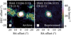 |
Fig. 1 CS .J = 2−1 emission at 97.98 GHz towards IRAS 15194–5115, in a 3.3 km s−1 wide channel centred on the systemic velocity. Left: archival data. Right: reprocessed data. The emission shown has been capped at 50 mlybeam−1 to make the low-level extended artefacts clearly visible. The white contours are at 5 mly beam−1. Synthesised beams are shown as filled black ellipses in the bottom left corner of each panel. |
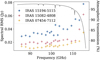 |
Fig. 2 rms noise in the spectra as a function of frequency. Each point denotes the average rms in a spectral window centred on the corresponding frequency. The black line is the atmospheric transmission at ALMA at 2 mm PWV. |
3.3 Data combination
For IRAS 15194–5115 and IRAS 15082–4808, observations with a higher spatial resolution (0″.4) were available in the ALMA archive (project code: 2015.1.01271.S, PI: Keller, D.), but covering only the frequency ranges 87.27–90.97 GHz and 99.14–102.89 GHz. The details of this dataset are given in Table 2. This dataset includes observations with both more extended (hereafter high-angular-resolution dataset) and more compact (hereafter low-angular-resolution dataset) baseline configurations compared to our data (hereafter intermediate-angular-resolution dataset). We therefore combined the corresponding visibilities from this project with our observations to increase the sensitivity to the emission on compact and extended spatial scales. This helped to increase the MRS of the observations, enabling us to recover the weak, extended molecular emission on large spatial scales that could have been filtered out due to the lack of very short baselines in the intermediate resolution data before combination, while also lowering the rms noise in the combined maps. The data combination was performed using the task concat in CASA version 6.3.0-48. Figure 3 shows the combined visibilities towards IRAS 15082–4808, depicting the extended and compact baseline coverages added.
As these two datasets were observed several months apart, it can be argued that they might not be compatible due to a possible time variation in the sources related to (1) the evolution of the ejected material and (2) changes in the molecular excitation. We note that any spatial variation in the circumstellar gas distribution occurring during the interval between these observations (≤ 1 yr) will be far below the spatial resolution of both datasets. For example, in the case of IRAS 15194–5115, given the expansion velocity of 21.5 km s−1 at a distance of ~696 pc (Table 1), the increase in angular size in 1 year is only 6 mas, around two orders of magnitude less than the angular resolution of the observations. In contrast, by comparing the line intensities from the two epochs used in the data combination, we do detect line variability likely connected to the variability in the stellar radiation field in two species, C2H and HC3N, for both IRAS 15194–5115 and IRAS 15082–4808. The observed variability is quantified in Sect. 4.2, and its impact on our results is discussed in Sect. 5. We still combine the two datasets for these lines, in order to trace the spatial structure in as much detail as possible, while increasing the uncertainty in the line intensities of these species by the observed percentage of variability.
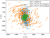 |
Fig. 3 uv plane of the combined observations towards IRAS 15082–4808 in the frequency range 87.2–89.1 GHz. The data from project 2015.1.01271.S has both long (orange) and short (green) baseline configurations, which help to better recover the compact and extended emission, respectively, compared to our original observations. |
4 Analysis and results
4.1 Line detection and identification
Continuum maps were produced from the line-free channels across the survey bandwidth (85–116 GHz) using multi-frequency synthesis (Rau & Cornwell 2011). The continuum emission is spatially unresolved for all three stars. The peak positions and total flux of the continuum maps are given in Table 4. The continuum was then removed from the data to obtain the continuum-subtracted line spectra.
Figure 4 shows an overview of the ALMA Band 3 spectra for all three stars. The full line-labelled ALMA Band 3 spectra of the three sources, extracted by integrating the intensity in a circular aperture of 12.5″ radius centred on the respective continuum peaks, so as to recover emission from all molecules, are presented in Appendix A. We used the Weeds (Maret et al. 2011) package in GILDAS4 to identify the emission lines. The Cologne Database for Molecular Spectroscopy (CDMS5; Müller et al. 2005) catalogue was referred to for line identification. Splatalogue6 (Remijan et al. 2007) was also used as an interface to obtain spectral line parameters. We detect, above the 3σ noise level, a total of 314 spectral emission features across the three stars, out of which 311 could be identified and assigned to 132 known rotational transitions of 49 molecular species, including various isotopologues (see Fig. A.1 and Table B.1). All detected lines, along with the associated spectroscopic parameters and observed integrated intensities towards the three stars, are tabulated in Table B.1. Figures in Appendix C show the brightness distributions at the systemic velocity and the spectra of the detected lines.
Most of the detected spectral lines are thermal emission lines from transitions in the vibrational ground states. However, some of the lines we detect, including HCN ν2 =2, J = 1−0, l = 0 and ν2 = 1, J =2−1, l =1, are known to display maser emission towards carbon stars, including IRAS 15082–4808 (e.g. Guilloteau et al. 1987; Smith et al. 2014; Menten et al. 2018; Jeste et al. 2022). We find both these lines to be masering towards all three stars in our observations as well, based on their extremely narrow line widths and significantly different line shapes in comparison to other non-masering lines. These maser lines are not a target of study in this paper and are not considered in the morphological or abundance analysis presented below. In addition, SiS maser action has been reported for v = 0 rotational lines towards IRC +10216 using 3D radiative transfer modelling based on mm observations (Fonfría et al. 2018). In the SiS lines that we detect in our ALMA/APEX surveys, there are no apparent maser spikes. In this work, we have therefore assumed that all of the observed SiS line emissions are of a primarily thermal nature. We will come back on this issue in a forthcoming radiative transfer analysis. Two of the three unidentified features in our data, at 86.886 and 100.407 GHz, present narrow line profiles (Fig. C.108), indicating that they could be masers and/or originate in the inner parts of the CSE.
Owing to the increased sensitivity and better coverage of spatial scales in the combined data (see Sect. 3.3), we detected several additional lines, including lines from C5H, C6H, C2S, and 1-C4H2, which were not detected in the intermediate resolution data alone. Further, the emission maps of several lines, including those of HC3N, HCN, HNC, C3N, and their 13C isotopologues, were enhanced by the data combination (e.g. Figs. C.21, C.25, C.27, C.34, C.69), owing to the same reasons as above.
We report the first detections of lines of 29SiO, 30SiO, 29SiS, 30SiS, Si34S, and C33S towards the three sources. The source with the largest number of detections is IRAS 15194–5115, presenting lines from 119 rotational transitions, compared to the 56 and 67 of IRAS 15082–4808, and IRAS 07454–7112, respectively (see Table B.1). This is largely due to the high abundance of 13C in its CSE, which leads to a large number of molecules containing 13C atoms, most of which are not detected towards the other two stars. We report the first detection of Si13CC, and doubly 13C-substituted isotopologues of HC3N towards IRAS 15194–5115, along with the long-chain hydrocarbons C6H, C8H, 1–C4H2, which have not been detected towards this source in previous observations.
Details of continuum emission.
4.2 Line variability
The two datasets used for data combination (Sect. 3.3) were observed several months apart (see Table 2). Hence, to check for potential variability, we compared spectra produced from a subset of visibilities that have the same uv-coverage in both datasets. This removes any difference in amplitudes caused by the larger uv-coverage of one of the datasets, and would reflect only time-dependent amplitude variations, connected to the variability in the stellar radiation field.
Owing to the 10% absolute calibration uncertainty of our data (see Sect. 3.2), and the ALMA Band 3 standard calibration uncertainty of 5%7 for the high- and low-angular-resolution datasets (see Sect. 3.3), we estimate a relative calibration uncertainty of ~11% between the two observations. For both IRAS 15194–5115 and IRAS 15082–4808, we find differences in line intensity greater than the relative calibration uncertainty for only two species, C2H and HC3N. For IRAS 15194–5115, we find a ~ 15–20% change in the integrated line intensity of the strongest hyperfine component of the C2H, N =1−0 line, and a change of ~10–15% in the HC3N, J = 11−10 line. For IRAS 15082–4808, we find a ~25–30% change for C2H, N =1−0, while for HC3N, J = 11−10, the change is ~10–15%. The phase of the variability is also opposite for C2H and HC3N (see Sect. 5 for a brief discussion of the detected variability in comparison with that found in IRC +10216).
4.3 Morphological diversity
Estimation of the extents of the emitting regions is needed in order to calculate molecular fractional abundances and constrain the chemical models. Fourteen species (see Table 5) were found to have non-blended lines with sufficiently high signal-to-noise ratios (≥3σ) in the channel maps to allow extracting information about the spatial distributions of the emission towards all three stars by producing azimuthally averaged radial profiles (hereafter AARPs; see Sect. 4.3.2) of the line brightness distributions.
Four of these species, HCN, SiO, SiS, and CS, have line brightness distributions that peak close to the central star and extend radially outwards (Fig. 5, top panel and Figs. C.10, C.21, C.35, C.60). These molecules are termed centrally peaked species. These encompass the so-called parent molecules formed in the stellar photosphere or the extended atmosphere, or molecules formed through circumstellar chemistry in the inner layer of the CSE (see Millar & Herbst 1994; Cordiner & Millar 2009; Agúndez et al. 2017, Agúndez et al. 2020). Eight species, C2H, C3H, C4H, c-C3H2, CN, C3N, HC5N, and HNC, present brightness distributions in the form of rings at the systemic velocity (e.g. Fig. 5, bottom panel and Figs. C.14, C.18, C.24, C.34, C.53, C.61, C.101). Our observations indicate that these species are distributed around the stars as hollow spherical shells with widths and peak radii that vary between molecules and stars. Hereafter we call these molecules shell species. The shell species are daughter molecules formed in the external layers of the CSE (see Agúndez et al. 2020) from centrally peaking parent molecules by photodissociation (e.g. C2H and CN) or due to photo-induced chemistry (e.g. HNC and HC5N), either directly or through series of intermediate steps (e.g. Daniel et al. 2012; Agúndez et al. 2017). Two species, HC3N and SiC2, show compound brightness distributions that have both centrally peaked and shell characteristics (Fig. 6, top-left panel and Figs. C.45, C.69). Maps of the emission at the systemic velocity for all the above species are shown in Appendix C.
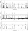 |
Fig. 4 ALMA Band 3 spectra extracted using a 12.″5 radius aperture centred on the star, for IRAS 15194−5115 (top), IRAS 15082−4808 (middle), and IRAS 07454−7112 (bottom). The spectrum in the lower panel for each star is capped at a low flux density limit to reveal the weaker emission lines. |
Extents of the emitting regions of selected molecular species.
4.3.1 Complex morphology in the CSEs of IRAS 15194–5115 and IRAS 15082–4808
The systemic velocity brightness distributions of HC3N, SiC2, HNC, and C2H towards IRAS 15194–5115 and IRAS 15082–4808 are shown in Fig. 6. The lower spatial resolution in the maps of IRAS 07454–7112 limits the detection of any similar substructure around this star. The maps in Fig. 6 have been produced by stacking the systemic velocity emission from all detected transitions in the ALMA Band 3 for each of these molecules. We regridded the line cubes to be stacked to ensure that they have the same spectral resolution (3.3 km s−1) and velocity grid, and used the software LineStacker (Jolly et al. 2020) to stack the cubes to extract the rms-weighted mean emission of the channels centred on the systemic velocity for each molecule. No channel averaging was performed as it would lead to the substructure visible at the systemic velocity to be smeared out. The spatial profiles obtained through radial cuts at different position angles on these maps are shown in Figs. 7 and 8.
For IRAS 15194–5115, the maps in Fig. 6 reveal well-defined arc structures within the emitting shell at the same locations in the HC3N and SiC2 maps. The approximate radial coincidence of the arcs seen in HC3N and SiC2 emission towards IRAS 15194–5115 can also be seen from the spatial profiles in Fig. 7. However, the SiC2 emission does not appear to fully trace the HC3N emission towards the southwest part of the image, and also around position angle (PA) ≈ 110° (Fig. 6, top-left panel). This could be due to the higher sensitivity of the HC3N data as compared to those of SiC2, since we have an HC3N line in the combined dataset (Sect. 3.3) with better uv-coverage than in the case of SiC2. Clumpiness cannot be ruled out either as a potential cause of this difference, as there exist significant differences in the chemical pathways of the two species. The C2H emission presents a main shell and a faint extended arc at larger radii (~10″), from the north down to the northeast part of the map. The same arc is traced by the HNC emission as well (Fig. 6, bottom-left panel), though this is somewhat hidden in the figure by the C2H contours. Notably, there is C2H and HNC emission visible even in areas between the arcs of the HC3N and SiC2 emission, towards IRAS 15194-5115 (Fig. 6, middle-left and bottom-left panels). The maps of the lines of C2H and HNC have a higher sensitivity in comparison to the SiC2 maps, as they are imaged from the combined data, and thus recover emission on more spatial scales.
In the case of IRAS 15082–4808, the SiC2 emission appears confined to only the main shell region of the HC3N map, and does not trace the outer arcs seen in the HC3N emission (Fig. 6, top-right panel). This could be due to the lower signal-to-noise ratio of the SiC2 maps, as in the case of IRAS 15194–5115. However, C2H and HNC trace both the main shell and the arcs to the southwest in the HC3N image (Fig. 6, middle-right and bottom-right panels).
4.3.2 Azimuthally averaged radial brightness profiles
Despite the complex morphology seen for some of the molecular line emissions, we used AARPs to study the radial structure of the emission for all sources, as is discussed below. This is the strategy used also by Agúndez et al. (2017) in their study of IRC +10216.
To obtain the inner (Ri) and outer (Re) radii of the line-emitting regions for different species, we constructed the mean AARPs (Appendix D) for the 14 molecules listed in Table 5. Several detected isotopologues of HCN, CS, SiO, and HC3N13(H13CN, 13CS, C34S, 29SiO, H13CCCN, HC13CCN, and HCC13CN) present emission with signal-to-noise ratios >3σ in their channel maps. Since the photodissociation of these molecules occurs throughout the broadband continuum (van Dishoeck 1988), and is not limited to narrow frequency ranges of discrete UV lines, their rarer isotopologues are expected to be present in the same spatial range as the main counterparts. Hence, to generate the mean AARPs for these species, we have averaged together emission from the detected lines of their non-blended isotopologues where such averaging increases the signal-to-noise ratio of the resulting profile.
Non-blended line cubes for a given species were convolved to a common circular beam with a size equal to the largest major axis among the individual beams. For each of these common-beam cubes, the emission from within a range of ±20% of the expansion velocity centred on the systemic velocity was averaged together to increase the signal-to-noise ratio, as we were now focusing on the overall size of the emitting shell and not the substructure within. The resulting maps were divided into successive concentric circular rings of increasing radii, centred on the continuum peak, with widths equal to the common restoring beam. The emission within each shell was averaged to obtain the azimuthally averaged brightness at the corresponding radius. These average brightnesses were plotted against the radii of the corresponding shells to produce one AARP per line. The uncertainty in the radial average for each shell corresponds to the rms noise in the channel map divided by the square root of the number of beams in the respective shell. The mean of these individual line AARPs was calculated for each species, weighted by the reciprocal of the squared uncertainty, to obtain the mean AARPs of the species shown in Fig. 9.
As part of this method, we verified for each species that the different transitions of all isotopologues are emitted from the same region around the central star. Fewer pixels were used in the azimuthal averaging as we calculated the AARP closer to the centre. This increased the chance that noise at the innermost radii might not be effectively suppressed, and could give rise to artefacts that need not correspond to actual emission. This is the reason why the error bars increase in size towards the inner part of the AARPs.
In order to estimate the radial extents of the emitting regions, the mean AARPs of each molecule were fitted with Gaussian profiles. We believe that Gaussian fits to the AARPs provide a reasonable way to systematically estimate the extent of the various emitting regions, to a first approximation. For instance, Fig. 10 shows such fits for the HCN and CN AARPs of IRAS 07454–7112. The Gaussian fits to the AARPs of the 14 selected species for all three sources are shown in Appendix D. The common restoring beam was used to obtain the beam-deconvolved sizes of the brightness distributions. For centrally peaked morphologies, the peak position (Rp) of the emission, and hence the inner radius (Ri), was set to 0. In this case, the outer radius (Re) is estimated as the half width at half maximum (HWHM) of the Gaussian fit to the mean AARP. In the case of shell emission, the inner and outer radii of the emission regions are given by the half maxima points on either side of the peak position of the Gaussian fit to the AARP. For each molecule, the aperture from which line spectra were extracted was set to a circular region with a radius equal to the peak position + 3σ of the Gaussian fit to the AARP (i.e. Rp + 2.5×HWHM) of the corresponding molecule, in order to extract the maximum amount of emission while including only a minimum number of pixels with only noise and no emission.
Figure 11 shows the radial extent estimates of the average brightness distributions of each of the 14 analysed molecules, calculated using the Gaussian fits to their mean AARPs, as was discussed above. The observed values on an angular scale have been converted to a spatial scale using the distances provided in Table 1. The values of Ri and Re, and the corresponding uncertainties are tabulated in Table 5. We present the qualitative results of the morphological analysis below, taking into account the calculated uncertainties.
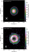 |
Fig. 5 Examples of centrally peaked (top) and shell (bottom) morphologies. Maps show the emission at the systemic velocity from the HCN (1 − 0) line (top) and the CN (1 − 0, hyperfine components stacked) line (bottom) towards IRAS 07454–7112. Contours are at 3, 5, and 10 σ, where σ refers to the rms noise in the emission maps (σ = 1.9 mJy beam−1 (HCN), 1.2 mJy beam−1 (CN)). The red + denotes the stellar position (continuum peak). |
4.3.3 Centrally peaked species
The AARPs of the centrally peaked species (SiO, SiS, CS, HCN) show clear deviations from a Gaussian profile in both IRAS 15194–5115 and IRAS 15082–4808, whereas they are fit well using Gaussians for IRAS 07454–7112 (an effect of the lower spatial resolution in this case; see Figs. D.1, D.2 (right), and D.3 (left)). For IRAS 15194–5115 and IRAS 15082–4808, the emissions from these molecules peak sharply at the centre and then gradually fall off at larger radii. Due to this, the Gaussian fits underestimate the radii of the actual emitting regions, as can be seen from Figs. D.1, D.2 (right), and D.3 (left).
The SiO and SiS emission regions are roughly co-spatial in each source. The CS emission region is more extended than those of SiO and SiS, while the HCN emission is the most extended of the centrally peaked species for all stars (see Fig. 9).
4.3.4 Shell species
Hydrocarbons: Within the calculated uncertainties (see Table 5), the shells of C2H and C4H peak at the same radii (Fig. 9) and have the same widths (Fig. 11) for the three stars, possibly with the exception of IRAS 15082-4808, where the C2H emission appears to extend further out than that of C4H by roughly 10% (see Table 5). The main hydrocarbon shells are of roughly the same thickness (~5500 AU) towards IRAS 15194–5115 and IRAS 15082–4808, but there are cases of faint extended emission beyond the main shell up to around 9300 AU for IRAS 15194–5115 (Fig. 9). IRAS 07454-7112 presents much thinner shells for the hydrocarbons, with a thickness of only ~1300 AU (Table 5). C5H, C6H, and C8H have also been detected towards IRAS 15082–4808 and/or IRAS 15194–5115 in the combined data, but the lines are too weak for any morphological information to be extracted.
Cyanides: In addition to the expected shell emission (see e.g. Agúndez et al. 2017, for the HC3N shell distribution for IRC + 10216), HC3N also shows significant central emission components towards all three stars. This is discussed in more detail in Sect. 4.3.5. In the cases of IRAS 15082–4808 and IRAS 07454–7112, the shell-HC3N and HC5N emissions trace roughly the same radial range (Fig. 11 and Table 5), and peak at around the same distance from the centre (Fig. 9). In the case of IRAS 15194–5115 the HC3N emission appears to peak at a slightly smaller radius than the HC5N emission, by ~30% (Fig. 9). However, this could be due to contamination from the central component of the HC3N emission and the low signal-to-noise in the HC5N maps towards this star. Compared to C2H and C4H, the HC3N and the HC5N emissions peak at slightly smaller radii in all three CSEs, by an estimated 10–40% (Fig. 9).
In general, CN, HNC, and the hydrocarbons present the most extended emission among the observed molecules. The peaks of the CN and C3N emissions are located roughly at the outer edges of the HCN and the shell-HC3N emissions, respectively (Figs. 9, 11 and Table 5). The CN AARP of IRAS 15194–5115 shows a secondary peak at larger radii (~11″, Fig. 9), which is not present in the other two stars. For IRAS 15194–5115, we also see weak emission structures at roughly the same location as the CN secondary peak in SiC2, HNC, C3N, C2H, C4H, and possibly C3H (Fig. 9). The fact that these arcs are traced by multiple species suggests that they are most likely the result of density enhancements (see also Sect. 5). The radial range of the HNC emission is roughly coincident with that of the C2H and C4H emission for all three stars (Fig. 11).
SiC2: SiC2 is the only silicon-bearing molecule out of the species studied in this paper that emits in a shell, whereas the others (SiO and SiS) are centrally peaked. The peak of the SiC2 emission is close to those of the HC3N and HC5N emissions for all three stars (Fig. 9). However, SiC2 also presents a central component that is further discussed below. We note that towards IRAS 15082–4808, the SiC2 AARPs show negative dips at larger radii (see Fig. 9), which is evidence of interferometric filtering out of extended emission. A similar behaviour is exhibited by C4H towards both IRAS 15194–5115 and IRAS 15082–4808, and possibly by HC5N towards IRAS 15194–5115.
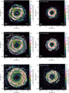 |
Fig. 6 Average brightness distributions, in a 3.3 km s−1 wide channel centred on the systemic velocity, of selected molecules towards IRAS 15194–5115 (left panels) and IRAS 15082–4808 (right panels). The names of the species whose emissions are shown in colour and contours are given in the bottom right corner of each panel in green and white, respectively. The synthesised beams of the colour maps and contours are shown as filled and hollow ellipses, respectively, in the bottom left corner of each panel. Contours are from 3σ to 15σ in intervals of 1σ. The σ values of the contour maps are, for IRAS 15194–5115, SiC2: 0.68 mJy beam−1 and C2H: 0.50 mJy beam−1, and, for IRAS 15082–4808, SiC2: 1.1 mJy beam−1 and C2H: 0.31 mJy beam−1. The red + denotes the stellar position (continuum peak). Red circles of radius 2.″5, 5.″0 and 7.″5 are drawn on each map to facilitate comparisons. |
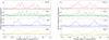 |
Fig. 7 Brightness distributions of HC3N, SiC2, C2H, and HNC, in a3.3 km s−1 wide channel centred on the systemic velocity of IRAS 15194–5115, along a line that intersects the star at PA = 0° (left) and PA = 90° (right). These profiles were extracted from radial cuts using the stacked images shown in Fig. 6. The horizontal shaded region of each profile shows the rms noise of the corresponding emission map. |
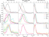 |
Fig. 9 Normalised AARPs of molecular line brightness distributions for IRAS 15194–5115 (left), IRAS 15082–4808 (middle), and IRAS 07454–7112 (right). The vertical grey gridlines apply to the lower x axis in cm units. |
4.3.5 Central emission components of HC3N and SiC2
For IRAS 15194–5115 and IRAS 15082–4808, HC3N and SKC2 show central components above the respective 3σ noise levels (Fig. 9). We stress that what we call central emission need not necessarily originate in the extended atmosphere, but can instead emanate from roughly anywhere within a synthesised beam (~700 AU for IRAS 15194–5115 and ~1000 AU for IRAS 15082–4808, see Table 2) centred on the star. The central components of these species can be seen in the spatial profile plots shown in Figs. 7 and 8 also. We note that even though C2H appears to have a central component towards IRAS 15082–4808 (see Fig. 6, middle-right panel and Fig. 8), this is due to the contamination from the blended hyperfine components of C2H, and potentially also weak lines of c-C3H2 and C6H (see Fig. A.1). In the case of IRAS 07454–7112, the angular resolution compared to the size of the emitting region is too poor to draw any conclusions about the behaviour of the brightness distributions in the inner part of the CSE. The possible formation mechanisms of these central components are discussed in more detail in Sect. 5.
4.4 Column density and rotation temperature estimates
We produced population diagrams (also referred to as rotation diagrams) to obtain the rotational temperature (Trot) and the column density (Ntot) for molecules with detected lines from three or more rotational transitions. We made a first-order correction for the optical depths. The method is described in detail in Appendix E.1. The minimum and maximum line optical depths of each molecule for which we have made population diagrams are listed in Table E.1. In this section, we present the column densities and rotation temperatures obtained from the population diagram analysis. All the population diagrams produced are shown in Figs. E.1–E.18. The rotational temperatures and column densities thus obtained are tabulated in Table 6 and shown in Fig. 12.
As the centrally peaked species are located close to the star, they are expected to have relatively high rotational temperatures. However, for all centrally peaked species, except SiS, the population diagrams yield much lower temperatures than expected (~ 10–20 K; Fig. 12, left panel). This is most likely due to three effects: (1) the limited range of energy levels covered (e.g. the highest energy level observed for HCN is at ~42 K, see Table B.2), where, in particular, high-excitation transitions are missing, yielding only a very limited sampling of the excitation properties, (2) the contribution from different lines may come from different regions based on their excitation conditions, and thus may not sample regions with the same temperature, and (3) the assumption of optically thin lines is not always fulfilled. For the SiS emission, where the energy range covered is larger, we obtain a somewhat higher rotational temperature of ~40 K.
The shell species often cover a large range of energy levels (e.g. 20–187 Κ for C4H, see Tables B.1 and B.2), and the emission from different lines of a species come from roughly the same region. They are therefore are expected to produce reliable estimates of rotation temperatures. HC3N and HC5N yield rotation temperatures in the range of 15–30 K, whereas C4H and C3N give slightly higher temperatures, around 30–45 K. Based on these results, we use rotational temperatures of 40 and 20 Κ for centrally peaked and shell species, respectively, in the abundance estimates based on single lines in Appendix E.3. We also note that, in general, the obtained rotational temperatures are highest for IRAS 07454–7112 (Fig. 12, left panel).
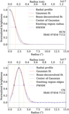 |
Fig. 10 Examples of Gaussian fits to the AARPs: HCN (centrally peaked species, top panel) and CN (shell species, bottom panel), both towards IRAS 07454–7112. The solid blue lines show the mean AARPs and the dashed red lines show the Gaussian fits. The dash-dotted black Gaussians were obtained by deconvolving the beam from the Gaussian fit. The yellow lines show the HWHM distance from the centre of the beam-deconvolved Gaussian on either side of the peak, and the horizontal pink linse depicts the HWHM (for centrally peaked emission, top panel) or the FWHM (for shell emission, bottom panel) of the beam-deconvolved Gaussian. |
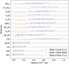 |
Fig. 11 Estimates of the extents of the molecular line-emitting regions. The horizontal lines show the radial extent of the emitting regions, as determined through Gaussian fits, for each molecule towards IRAS 07454–7112 (yellow), IRAS 15082-4808 (red), and IRAS 15194–5115 (blue). The ♦ signs denote the positions of the emission peaks. The + signs indicate species for which the emissions from several isotopo-logues (see Sect. 4.3.2) were averaged to produce the AARP. The values of the emission extents and their uncertainties are listed in Table 5. |
4.5 Abundance estimates
For the species for which we could produce population diagrams (see Table 6 and Appendix E), we calculated fractional abundances from the corresponding column densities, using Eq. (E.6). For all the other species, we obtained a rough estimate of the abundance analytically using Eq. (E.7). These two methods are described in Appendix E.
The fractional abundances estimated towards our stars are listed in Table 7 and shown in Fig. 13, along with the corresponding abundances for IRC +10216 obtained from the literature. We also show the abundances normalised with those of IRC +10216, for an easier source-to-source comparison, and normalised to each star’s C34S abundance, to eliminate source-specific uncertainties on distance and MLR. We chose C34S in particular, since the S and34 S abundances are not expected to vary between the sample stars, nor with respect to IRC +10216 (Henry et al. 2012). Whereas we find similar CS abundances for all of the stars, we note that Massalkhi et al. (2019) have reported a decreasing CS peak abundance for increasing density in carbon-rich CSEs.
We made first-order corrections for optical depths, which are particularly significant for HCN, SiO, and CS. However, the estimated rotational temperatures are much lower than expected for these centrally peaked species (see Table 6 and Fig. 12, left panel), and we therefore believe that for these species the reported abundances are lower limits.
The abundances of the shell species are in general comparable, within the uncertainties, in the three stars. Since extended emission appears to have been resolved out for SiC2 and C4H towards IRAS 15194–5115 and IRAS 15082–4808 (see Sect. 4.3.4), the ALMA points in the population diagrams of these species for these sources could be slightly underestimated.
We do not expect this to change the abundances beyond the estimated uncertainties.
Rotation temperatures and column densities obtained using population diagrams.
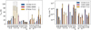 |
Fig. 12 Rotation temperatures (Trot, left panel) and total column densities (Ntot, right panel) obtained from population diagrams. The dashed vertical black line separates the shell species and the centrally peaked species. |
Uncertainties of abundance estimates
The accuracy of a determined absolute abundance depends on the method used to estimate it, the validity of the assumptions that went into the calculations, and the uncertainties of the input parameters. We have assumed a simple circumstellar model (including the shape of the radial abundance distributions), and excitation in LTE of the molecular energy levels. Among the input parameters, we have the adopted distances and the mass-loss rates. In addition, the amount and quality (including calibration uncertainties) of the observational data contribute to the uncertainty, through the measured fluxes and estimated emitting-region sizes. This makes it difficult to estimate formal errors of the abundances.
The arcs seen in the molecular emission towards IRAS 15194–5115 and IRAS 15082–4808 suggest that there are density enhancements (see Sect. 4.3.4). These are not considered in the assumed smooth H2 flow, as we do not have a well-constrained quantitative estimate of these enhancements.
This also adds to the uncertainty of the abundance estimates. Attempts to address this demand entailed modelling that is outside the scope of the present work.
In general, we estimate that the overall uncertainty, including all parameters and model assumptions, is about a factor of three to five for the absolute abundances estimated using population diagrams, depending on the quality of the population diagram. The single-line estimates are, at best, order-of-magnitude estimates. The uncertainty decreases to a factor of two to three and a factor of five in the cases of population diagram and single-line estimates, respectively, when comparing abundances that are normalised individually to the respective C34S abundance for each source (Sect 4.5), since this means that the influences of distance, mass-loss rate, and the circumstellar model to a large extent are removed. The comparison abundances adopted for IRC +10216, which were obtained using different methods, have an uncertainty of at least a factor of two to three.
Molecular fractional abundances.
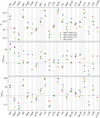 |
Fig. 13 Molecular fractional abundances for the three stars (this work) and IRC +10216 (from the literature, see Table 7). The absolute abundances are shown in the top panel. The middle panel shows the abundances normalised to IRC +10216, and the bottom panel shows the abundances normalised to each star’s own C34S abundance. Uncertainties of these estimates are discussed in Sect. 4.5. |
Isotopic ratios.
4.6 Isotopic ratios
Stellar elemental isotopic ratios are measures of the nucleosynthetic history (including dredge-up) of a star, and are, as such, important observational results. Spectral lines from our data can be used to estimate circumstellar isotopologue ratios. In most cases, there is every reason to think that these are also good estimates of the corresponding stellar isotope ratios, since the different isotopologues are produced, destroyed, and excited in a similar way, to first approximation. This applies, for instance, to silicon and sulphur. For carbon, the situation is special since the photo-dissociation process is isotope-selective in the case of CO (Saberi et al. 2019). However, the effect of this is estimated to be small for high-mass-loss-rate objects (Saberi et al. 2020), that is, the type of stars in this study.
For species for which we could make reliable population diagrams, the isotopic ratios were calculated from the abundance ratios of the relevant molecules. For all other species, the isotopic ratio was determined by calculating the corresponding line intensity ratios. This method assumes that the J – J′ transition is excited under the same conditions for both isotopo-logues. We refrained from performing any frequency corrections on the isotopic ratios, as the uncertainties in the estimated ratios are significantly greater than the magnitude of such corrections. We present estimates of the isotopic ratios for the three stars in Table 8, along with isotopic ratios for IRC+10216 and the Sun obtained from the literature for comparison.
Carbon: The 12C/13C ratios calculated from the optically thin lines of HNC, SiC2, HC3N, C4H, and C3N for all three stars are consistent with their respective values obtained from the CO radiative transfer modelling by Woods et al. (2003), though the C4H ratio is slightly larger than the others.
Silicon: The 28Si/29Si, 28Si/30Si, and 29Si/30Si values in the three stars are similar to the expected values of 20, 30, and 1.5, the solar values (Asplund et al. 2009).
Sulphur: The 32S/33S and 32S/34S values, about 100 and 20, respectively, in the three stars, are close to the expected solar values of 125 and 22.
5 Discussion
A comparison of molecular radial brightness distributions and abundances between the three stars and with IRC +10216 enables us to understand whether and how the chemistry in C-type AGB CSEs is affected by variations in properties including the MLR and the stellar 12C/13C ratio. We compared the molecular radial brightness distributions of various molecules, focusing on Figs. 9 and 11 and the molecular abundances based on Fig. 13. Even though the AARPs show only the radial structure of the emission and average out all azimuthal variations, they still provide valuable information on the chemical stratification in the CSE, and thereby on the formation and destruction mechanisms of various molecules.
We started by analyzing whether the spatial extents of the molecular CSEs follow that expected from photodissociation by an external UV radiation field. The photodissociation radius of a molecule depends on how well it is shielded from the interstellar radiation field (ISRF). This is determined by the outward column density of dust, which in turn depends on the mass-loss rate, or rather the circumstellar density (proportional to Ṁ/υexp), and also on the gas-to-dust ratio. The circumstellar density is lowest for IRAS 07454–7112, and about three and five times higher for IRAS 15194–5115 and IRAS 15082–4808, respectively (Table 1). The gas-to-dust ratios for the three sources are likely similar (Groenewegen et al. 1998). Thus, we expect the sizes of the molecular shells to be smallest for IRAS 07454–7112, larger for IRAS 15194–5115, and largest for IRAS 15082–4808. Indeed, the shells of IRAS 07454–7112 are by far the smallest ones, by about a factor of three (Figs. 9, 11, Table 5). However, those of IRAS 15194–5115 and IRAS 15082–4808 are of about the same size. They are also comparable in size to the molecular shells seen towards IRC+10216, which has a circumstellar density roughly three times higher than that of IRAS 15194–5115 and 1.5 times that of IRAS 15082–4808. This could be attributed to errors in the distances (which affect mass-loss-rate estimates and spatial extents), differences in the gas-to-dust ratio, differences in the circumstellar dust properties, and/or to the CSEs being exposed to slightly different strengths of the ISRF. Thus, our results, which are also corroborated by the radial brightness profiles of the centrally peaked species, are not inconsistent with the expected sizes of molecular distributions affected by photo-dissociation by UV light from the outside. The next paper in the series will address this in a more quantitative way (see Sect. 1). As mentioned above, the lower circumstellar density of IRAS 07454–7112 leads to the parent molecules being photodis-sociated closer to the star than in the other two sources. This may be reflected in the higher rotation temperatures obtained for the daughter species for this object (Fig. 12, left panel).
When looking at the AARPs of shell species in more detail, we conclude that the cyanopolyynes are located slightly inwards with respect to the hydrocarbons (see Figs. 9, 11 and Table 5). The average peak position of the cyanopolyynes falls inside that of the hydrocarbons by around 25–30% for both IRAS 15194–5115 and IRAS 15082–4808, and by roughly 10% for IRAS 07454–7112. We find no marked difference in the locations among the species of these respective groups. The largest spatial extents are found for HNC, CN, and possibly C3N, and the hydrocarbons C2H and C4H. This is consistent with the results of Daniel et al. (2012) and Cernicharo et al. (2013), who found HNC emission extending to more than 30″ towards IRC +10216, and Agúndez et al. (2017), who found CN to present emission to similar radii, extending beyond that of the other cyanides and cyanopolyynes around this star. The shell of c-C3H2, detected only towards IRAS 15194–5115, appears roughly coincident with the C2H and C4H shells. In all of these respects, we reproduce the findings of Agúndez et al. (2017) in the case of IRC +10216. We note that, while Agúndez et al. (2017) find that the CN emission towards IRC +10216 clearly extends beyond that of the C2H and C4H radicals, we observe the faint extended emission from these radicals to have roughly the same radial extent as the CN towards IRAS 15194–5115 and IRAS 15082–4808 (Fig. 9). However, this is due to the most extended CN emission being filtered out due to the lack of very short baselines in our observations, in contrast to that of Agúndez et al. (2017), who used single dish observations to recover the flux filtered out by ALMA.
From our observations, we find that HC3N is present within one synthesised beam around two of our stars, corresponding to ~700 AU and ~1000 AU for IRAS 15194–5115 and IRAS 15082–4808, respectively. For IRC +10216, Siebert et al. (2022) find significant emission from high-excitation (J = 38 − 37, 30 − 29, 28 − 27) lines of HC3N within 350 AU from the star.
Herbst & Leung (1990), Howe & Millar (1990), and Agúndez et al. (2017) suggest that HC3N is formed in C-type CSEs mainly through the reaction
 (1)
(1)
Hence, it is expected to appear in the inner CSE if there is enough CN available. We cannot confirm this pathway as the main production channel, since we do not detect CN emission above the noise level in the innermost part in any of our CSEs. However, this could be a sensitivity effect, since the surface brightness of the CN emission is low at the systemic velocity for the two sources where we have sufficient spatial resolution to do this. Van de Sande & Millar (2022) suggest that a significant inner wind abundance of complex species, including HC3N, can be indicative of the presence of a white dwarf binary companion. However, according to their models, this will also lead to severely reduced SiO and SiS abundances, an effect not seen in our data.
We find that the SiC2 abundance distribution has both a central and a shell component. The presence of a central component has been discussed before by, for instance, Lucas et al. (1995); Fonfria et al. (2014); Velilla Prieto et al. (2015a); Massalkhi et al. (2018). It is most likely explained by SiC2 being formed in the extended atmosphere, as was already suggested by MacKay & Charnley (1999), and predicted by the chemical models of Agúndez et al. (2020). The detection of hot SiC2 ro-vibrational bands in the optical towards carbon stars (Sarre et al. 1996) supports this. The SiC2 shell, on the other hand, is expected to be formed due to the fast reaction of Si with C2H2 in the low-temperature (< 100 K) conditions prevalent in the outer parts of the CSE (Canosa et al. 2001; Cernicharo et al. 2010):
 (2)
(2)
Further out, it is photo-dissociated to form Si and C2 (Harada et al. 2010).
The arcs seen in the HC3N and SiC2 emissions at the systemic velocity for IRAS 15194−5115 are clearly co-spatial (Fig. 6, top left panel), though these molecules themselves do not share any common chemistry. These arcs appear to be traced by a variety of other molecules as well (Sect. 4.3.1). This suggests that the arc structures seen are, predominantly, the result of density enhancements rather than abundance variations. Such thin shells in various cyanopolyynes and hydrocarbons are also seen in the CSE of IRC +10216 (Agúndez et al. 2017). Additionally, for IRC +10216, Mauron & Huggins (1999, 2000); Leão et al. (2006), and Dinh-V-Trung & Lim (2008) showed that the clumpy shells seen in cyanopolyyne emission coincide spatially with the dust arcs observed in dust-scattered optical light, and hence represent the same density enhancements in the CSE. This is in line with the suggestion by Lykou et al. (2018), based on CO, SiO, CS, and HC3N emission and NACO/VLT near-infrared data, that IRAS 15194–5115 could be a binary system in which a spiral-like density structure would be imprinted in the CSE by an orbiting companion. Similar substructure was observed in CO, CN, and C4H towards IRC +10216 by Cernicharo et al. (2015); Decin et al. (2015) and Guélin et al. (2018), which was attributed to episodic mass loss triggered by the existence of a putative binary companion. Towards IRAS 15194–5115, we find emission from C2H also in the gaps between the arcs seen in HC3N (Fig. 6, middle-left panel and Fig. 7). This need not be contrary to the proposition of density-enhanced shells but can rather be explained by the larger impact of density enhancements on the abundance of HC3N (Cordiner & Millar 2009).
The rotation temperatures we estimate from our population diagrams match reasonably well with those estimated for IRC +10216. He et al. (2008) obtained a rotation temperature of 28 K for HC3N, and Cernicharo et al. (2000) reported 35 K for C4H and 20 K for C3N, which align with our estimates. We note that Pardo et al. (2022) also present population diagrams of C4H and HC5N, among other species, towards IRC +10216 using lines from their 31.0–50.3 GHz spectral survey. These yield rotation temperatures of 4.9 and 10.1 K, respectively, much lower than our estimates for these species (Table 6).
We have estimated that the uncertainties of the relative abundances when comparing our three stars are a factor of two to three for population diagrams and a factor of five for singleline estimates. When comparing with IRC +10216 they increase to a factor of five for population diagrams and a factor of ten for single-line estimates. Considering this, there are no significant differences or trends in the abundances among our three stars, other than the possibly lower hydrocarbon abundances in IRAS 07454–7112 compared to the other two stars (Fig. 13). The latter could be a result of the lower density of the CSE of IRAS 07454–7112. When comparing with IRC +10216, all abundances except that of SiO are within a factor of ten, meaning that, except for this species, we find no significant differences with the abundances estimated for IRC +10216. The SiO abundances in our stars are higher than that for IRC +10216 by an order of magnitude. The same discrepancy was observed by Woods et al. (2003) in their single-dish line survey of these sources. The putative over-abundance of SiO in our stars needs to be confirmed through a proper radiative transfer analysis.
Time variability of the intensity of thermal (non-maser) line emission has been reported for several species in the case of IRC +10216 (Cernicharo et al. 2014; Pardo et al. 2018; He et al. 2019). By comparing the observations from two epochs, we find variability in the 3 mm line emission of C2H and HC3N towards IRAS 15194–5115 and IRAS 15082–4808. Our findings (Sect. 4.2) are in line with the conclusions of Cernicharo et al. (2014) and Pardo et al. (2018), who show that C2H shows the highest variability at 3 mm, and that the phase of variability of the cyanopolyynes is opposite to that of C2H, for IRC +10216 as well. We note that, in addition to C2H and HC3N, Pardo et al. (2018) also found time variability in the lines of CN, C4H, C5H, and HC5N towards IRC +10216, which we are unable to ascertain for the stars in our sample from the current data. This could potentially be due to the intensity variation in the lines of these species being lower than the calibration uncertainty.
The three stars in our sample have significantly different inferred 12C/13C ratios (Table 8), with IRAS 15194–5115 standing out with a very low value of six. For this star, Ramstedt & Olofsson (2014) report a 12CO/13CO ratio of ten, slightly higher than the value of six estimated by Woods et al. (2003) and us (still within the uncertainties of both estimates). The other two stars, and IRC +10216, have values in the range of 20–50, which is consistent with typical AGB evolution models (see e.g. Lattanzio & Boothroyd 1997, and references therein) where the surface 12C/13C ratio increases as the star evolves along the AGB. This has also been traced by observations (e.g. Lambert et al. 1986; Abia et al. 2001; Ramstedt & Olofsson 2014). It cannot be concluded with certainty that the low ratio in IRAS 15194–5115 is due to hot-bottom burning (HBB) and a subsequent evolution to a carbon star, as the star may not be massive enough for HBB to occur. Whereas HBB efficiently produces N, we find no indications of any N enhancement in the circumstellar species for this star. It has been suggested that the presence of a hot binary companion may alter the circumstellar 12CO/13CO through differential photodissociation so that it differs from the atmospheric 12C/13C, whereas this is not the case for the isotopo-logues of the other observed molecules in this study (see Vlemmings et al. 2013; Saberi et al. 2019). They are therefore expected to give good estimates of the stellar 12C/13C ratio. The models by Izzard & Tout (2003), combining nucleosynthesis and binary star evolution, have shown that the atmospheric 12C/13C can be lowered significantly in the presence of binary companions.
Finally, the observed similarity of the silicon isotopic ratios with the respective solar values is in line with AGB nucleosynthesis in lower-mass stars (≲4 M⊙, Karakas & Lugaro 2016). In addition, the sulphur isotopic ratios being consistent with the corresponding solar ratios is in line with the fact that these isotopes are not expected to be influenced by nucleosynthesis in lower-mass stars (Shingles & Karakas 2013; Humire et al. 2020, and references therein).
6 Summary and conclusions
Our unbiased ALMA spectral survey mapped for the first time the 3 mm molecular rotational transitions in the CSEs of the C-type AGB stars IRAS 15194–5115, IRAS 15082–4808, and IRAS 07454–7112 at a high spatial resolution (0.″7-1.″7, corresponding to roughly 500–1000 AU). Extensive interferomet-ric surveys of this kind have previously been performed only towards IRC +10216. The survey yielded 311 identified lines (including hyperfine splitting components), from 132 rotational transitions of 49 molecular species, including various isotopo-logues, and three unidentified lines. Data with a sufficient signal-to-noise ratio (≳3σ in the emission maps), which enabled us to comparatively analyse the morphological characteristics across the three stars, was obtained for 14 species. We produced AARPs to obtain the radial brightness distributions of these species, and estimated the extents of their emitting regions. We used optical-depth-corrected population diagrams or single-line calculations to calculate the fractional abundances of these molecules and their less abundant isotopologues. Lines from our APEX single-dish surveys of the sources were used in the population diagrams to complement those from the ALMA observations. We also report several new detections towards these stars, namely 29SiO, 30SiO, 29SiS, 30SiS, Si34S, C33S, Si13CC, C6H, C8H, 1-C4H2, and doubly 13C-substituted isotopologues of HC3N.
We find deviations from a smooth, spherically symmetric CSE towards IRAS 15194–5115 and IRAS 15082–4808 in several molecules, and detect density enhancements similar to what has previously been reported in the CSE of IRC +10216, which might indicate the presence of stellar or substellar companions of these stars. The very low 12C/13C ratio and the presence of a “central” emission component for HC3N may also be indicative of the presence of a binary companion of IRAS 15194–5115.
By comparing our morphological results for the three sources amongst themselves and with results from the literature for IRC +10216, we find that the chemistry in the CSEs, as traced by the radial order in which different molecules exist around the central star, is very similar in our sources and IRC +10216. The chemistry does not seem significantly affected by the differences in the nucleosynthetic history of the individual stars, indicated by differences in their 12C/13C ratios, except for the expected increased abundance of singly and doubly 13C-substituted isotopologues in the CSE of IRAS 15194–5115, owing to its low 12C/13C ratio. We find that, within the uncertainties of our analysis, most of the estimated fractional abundances are similar across the source sample, and to the corresponding IRC +10216 values. The notable exception is SiO, which appears more abundant in the three stars in our sample in comparison to IRC +10216, by an order of magnitude. The calculated abundances of the shell species match reasonably well with the photochemical models for all sources. We also detect variability in the line emission of C2H and HC3N for two stars in our sample.
We estimated the carbon, silicon, and sulphur isotopic ratios for the three stars. The 12C/13C ratios match the values from the literature for all three stars, and the silicon and sulphur ratios of the three stars match reasonably well the corresponding IRC +10216 and solar values.
Overall, we conclude that the chemistry in the C-type AGB CSEs studied in this paper, as judged from radial brightness distributions and estimated abundances, is consistent across our small sample and with that of IRC +10216. This indicates that IRC +10216 serves reasonably well as an archetypal C-type AGB star, in terms of modelling C-type CSE chemistry, at least for MLRs within an order of magnitude of that of itself. However, we remind the reader of the possible binary nature of IRC +10216 and potentially also of some of the sources in our study. Binarity might influence the chemical properties differently for different sources, depending on the properties of the objects in the system.
Non-LTE radiative transfer modelling is necessary to more accurately determine the molecular abundances. This, and the subsequently updated chemical models, will be presented in a series of upcoming papers. More extensive observations, in terms of both sources and spectral coverage, are required to thoroughly constrain the chemical models and small-scale chemical variations in the CSEs. A detailed investigation of the morphology of the CSEs of the stars in our sample and the possible presence of binary companions will require observations with a higher angular resolution and sensitivity.
Acknowledgements
R.U. acknowledges data reduction support from the Nordic ALMA Regional Centre (ARC) node based at Onsala Space Observatory (OSO), Sweden. The Nordic ARC node is funded through Swedish Research Council grant No 2017-00648. E.D.B. acknowledges financial support from the Swedish National Space Agency. S.B.C. and M.A.C. were supported by the NASA Planetary Science Division Internal Scientist Funding Program through the Fundamental Laboratory Research work package (FLaRe). I.d.G. acknowledges support from grant PID2020-114461GB-I00, funded by MCIN/AEI/10.13039/501100011033. The work of M.G.R. is supported by NOIRLab, which is managed by the Association of Universities for Research in Astronomy (AURA) under a cooperative agreement with the National Science Foundation, USA. This paper makes use of the following ALMA data: ADS/JAO.ALMA#2013.1.00070.S, ADS/JAO.ALMA#2015.1.01271.S, ADS/JAO.ALMA#2011.0.00001.CAL. ALMA is a partnership of ESO (representing its member states), NSF (USA) and NINS (Japan), together with NRC (Canada), MOST and ASIAA (Taiwan), and KASI (Republic of Korea), in cooperation with the Republic of Chile. The Joint ALMA Observatory is operated by ESO, AUI/NRAO and NAOJ. This paper is based on observations with the Atacama Pathfinder Experiment (APEX) telescope. APEX is a collaboration between the Max Planck Institute for Radio Astronomy, the European Southern Observatory, and the Onsala Space Observatory. Swedish observations on APEX are supported through Swedish Research Council grant No 2017-00648. The APEX observations were obtained under project numbers O-0107.F-9310 (SEPIA/B5), O-0104.F-9305 (PI230), and O-087.F-9319, O-094.F-9318, O-096.F-9336, and O-098.F-9303 (SHeFI).
Appendix A ALMA Band 3 spectra
This appendix shows the entire ALMA Band 3 spectra of the three sources. The spectra were extracted by integrating the intensity in a circular aperture of 12.5″ radius centred on the respective continuum peaks, so as to recover emission from all molecules. Line detections (Table B.1) are labelled in the figure at the corresponding frequencies.
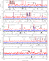 |
Fig. A.1 ALMA Band 3 line survey of IRAS 07454–7112 (black), IRAS 15082–4808 (blue; vertical offset of 0.1 Jy), and IRAS 15194–5115 (red; vertical offset of 0.2 Jy). Labels show the carrier molecule of the indicated emission. Red labels indicate tentative or unidentified detections, and green labels indicate lines that have been identified only in central-pixel spectra (not shown). The spectra from the combined data have been inserted in the respective frequency ranges (see Table 2). |
Appendix B Details of detected transitions
This appendix lists the detected emission lines along with their upper-level energies and integrated intensities for the three stars. Table B.1 presents the lines detected in the ALMA Band 3 spectra, and Table B.2 lists the lines from the APEX surveys (see Sect. 3.1) that were used in this work for abundance calculations.
Details of all detected transitions in the ALMA Band 3 survey.
Details of the lines from APEX observations used in the population diagrams.
Appendix C Emission maps and line spectra
The below figures show the line emission maps (top panels) averaged over ±20% of the expansion velocity around the systemic velocity, and the line spectra (bottom panels), for IRAS 15194–5115 (left), IRAS 15082–4808 (centre), and IRAS 07454–7112 (right). The figures are ordered in increasing order of line rest frequency, which is given in parentheses at the end of the figure caption. The white contours in the emission maps are at 3, 10, and 30 sigma. The synthesised beams are shown as filled white ellipses at the bottom left of each map. The grey shaded regions in the line spectra represent the channels used for calculating the integrated intensities of the lines, reported in Table B.1. The dotted vertical line in the line spectra marks the systemic velocity of the source. Missing plots indicate non-detection of the concerned line towards the particular source.
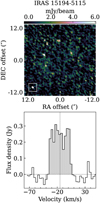 |
Fig. C.1 C13CCCH, N=9-8, J=19/2-17/2 (85.201906 GHz) |
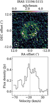 |
Fig. C.2 C13CH, N=1-0, J=3/2-1/2 (85.232792 GHz) |
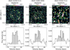 |
Fig. C.3 c-C3H2, 21,2–10,1 (85.338894 GHz) |
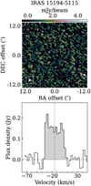 |
Fig. C.4 CC13CCH, N=9-8, J=17/2-15/2 (85.37033 GHz) |
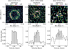 |
Fig. C.5 C4H, N=9-8, J=19/2-17/2 (85.634004 GHz) |
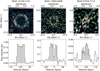 |
Fig. C.6 C4H, N=9-8, J=17/2-15/2 (85.672582 GHz) |
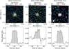 |
Fig. C.7 29SiO, 2-1 (85.759194 GHz) |
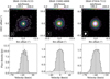 |
Fig. C.8 H13CN, 1-0 (86.339921 GHz) |
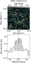 |
Fig. C.9 Si13CC, 41,4 – 31,3 (86.562636 GHz) |
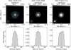 |
Fig. C.10 SiO, 2-1 (86.846985 GHz) |
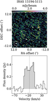 |
Fig. C.11 HN13C, 1-0 (87.090825 GHz) |
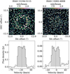 |
Fig. C.12 C2H, N=1-0, J=3/2-1/2, F=1-1 (87.284105 GHz) |
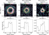 |
Fig. C.13 C2H, N=1-0, J=3/2-1/2, F=2-1 (87.316898 GHz) |
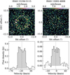 |
Fig. C.14 C2H, N=1-0, J=1/2-1/2, F=1-0 (87.44647 GHz) |
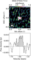 |
Fig. C.15 30SiS, 5-4 (87.550558 GHz) |
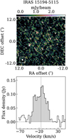 |
Fig. C.16 H13CC13CN, 10-9 (87.773712 GHz) |
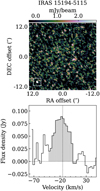 |
Fig. C.17 H13C13CCN, 10-9 (87.841102 GHz) |
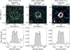 |
Fig. C.18 HC5N, 33-32 (87.86363 GHz) |
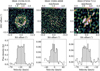 |
Fig. C.19 H13CCCN, 10-9 (88.166832 GHz) |
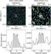 |
Fig. C.20 Si34S, 5-4 (88.285828 GHz) |
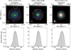 |
Fig. C.21 HCN, 1-0 (88.631602 GHz) |
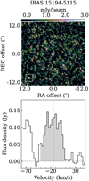 |
Fig. C.22 CC13CN, N=9-8, J=19/2-17/2 (88.7117 GHz) |
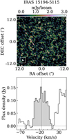 |
Fig. C.23 CC13CN, N=9-8, J=17/2-15/2 (88.7302 GHz) |
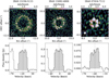 |
Fig. C.24 C3N, 9-8 (A) (89.0456 GHz) |
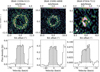 |
Fig. C.25 C3N, 9-8 (B) (89.0643 GHz) |
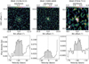 |
Fig. C.26 29SiS, 5-4 (89.103749 GHz) |
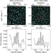 |
Fig. C.27 I-C4H2, 103,8-93,7 (89.289791 GHz) |
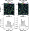 |
Fig. C.28 C6H, J=65/2-63/2 (90.093295 GHz) |
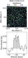 |
Fig. C.29 HC13C13CN, 10-9 (90.204324 GHz) |
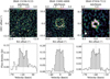 |
Fig. C.30 HC5N, 34-33 (90.52589 GHz) |
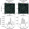 |
Fig. C.31 30SiC2, 40,4-30,3 (90.562283 GHz) |
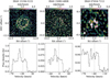 |
Fig. C.32 HC13CCN, 10-9 (90.593059 GHz) |
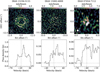 |
Fig. C.33 HCC13CN, 10-9 (90.601777 GHz) |
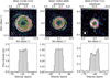 |
Fig. C.34 HNC, 1-0 (90.663568 GHz) |
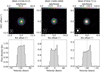 |
Fig. C.35 SiS, 5-4 (90.771564 GHz) |
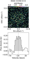 |
Fig. C.36 Si13CC, 40,4-30,3 (90.848527 GHz) |
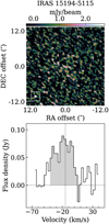 |
Fig. C.37 C8H, J=155/2-153/2 (90.92464 GHz) |
 |
Fig. C.38 HC3N, 10-9 (90.979023 GHz) |
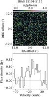 |
Fig. C.39 13CCCCH, N=10-9, J=21/2-19/2 (91.875516 GHz) |
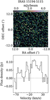 |
Fig. C.40 13CCCCH, N=10-9, J=19/2-17/2 (91.906057 GHz) |
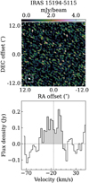 |
Fig. C.41 Si13CC, 42,3-32,2 (92.064397 GHz) |
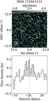 |
Fig. C.42 CCC13CH, N=10-9, J=21/2-19/2 (92.277495 GHz) |
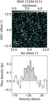 |
Fig. C.43 CCC13CH, N=10-9, J=19/2-17/2 (92.31491 GHz) |
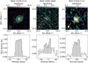 |
Fig. C.44 13CS, 2-1 (92.494308 GHz) |
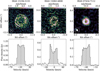 |
Fig. C.45 SiC2, 40,4-30,3 (93.063639 GHz) |
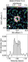 |
Fig. C.46 HC5N, 35-34 (93.188123 GHz) |
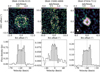 |
Fig. C.47 SiC2, 42,3-32,2 (94.245393 GHz) |
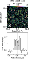 |
Fig. C.48 C13CCCH, N=10-9, J=21/2-19/2 (94.670583 GHz) |
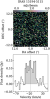 |
Fig. C.49 C13CCCH, N=10-9, J=19/2-17/2 (94.708235 GHz) |
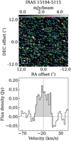 |
Fig. C.50 CC13CCH, N=10-9, J=21/2-19/2 (94.814724 GHz) |
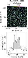 |
Fig. C.51 CC13CCH, N=10-9, J=19/2-17/2 (94.853126 GHz) |
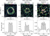 |
Fig. C.52 C4H, N=10-9, J=21/2-19/2 (95.150389 GHz) |
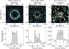 |
Fig. C.53 C4H, N=10-9, J=19/2-17/2 (95.188949 GHz) |
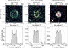 |
Fig. C.54 SiC2, 42,2-32,1 (95.579381 GHz) |
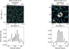 |
Fig. C.55 HC5N, 36-35 (95.850335 GHz) |
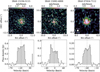 |
Fig. C.56 C34S, 2-1 (96.41295 GHz) |
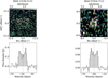 |
Fig. C.57 H13CCCN, 11-10 (96.983001 GHz) |
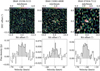 |
Fig. C.58 C33S, 2-1 (97.172064 GHz) |
 |
Fig. C.59 Si13CC, 41,3-31,2 (97.295257 GHz) |
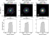 |
Fig. C.60 CS, 2-1 (97.980953 GHz) |
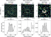 |
Fig. C.61 C3H, J=9/2-7/2 (98.01207 GHz) |
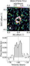 |
Fig. C.62 HC5N, 37-36 (98.512524 GHz) |
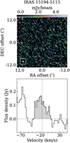 |
Fig. C.63 CC13CN, N=10-9, J=21/2-19/2 (98.569 GHz) |
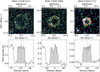 |
Fig. C.64 C3N, 10-9 (A) (98.94 GHz) |
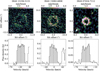 |
Fig. C.65 C3N, 10-9 (B) (98.9588 GHz) |
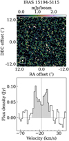 |
Fig. C.66 HC13C13CN, 11-10 (99.224259 GHz) |
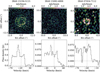 |
Fig. C.67 HC13CCN, 11-10 (99.651849 GHz) |
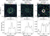 |
Fig. C.68 HCC13CN, 11-10 (99.661467 GHz) |
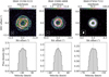 |
Fig. C.69 HC3N, 11-10 (100.076392 GHz) |
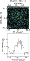 |
Fig. C.70 13CCCCH, N=11-10, J=23/2-21/2 (101.06306 GHz) |
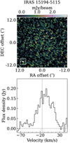 |
Fig. C.71 13CCCCH, N=11-10, J=21/2-19/2 (101.09403 GHz) |
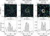 |
Fig. C.72 HC5N, 38-37 (101.174677 GHz) |
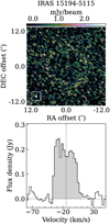 |
Fig. C.73 CCC13CH, N=11-10, J=23/2-21/2 (101.506343 GHz) |
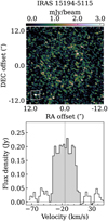 |
Fig. C.74 CCC13CH, N=11-10, J=21/2-19/2 (101.543766 GHz) |
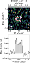 |
Fig. C.75 HC5N, 39-38 (103.836817 GHz) |
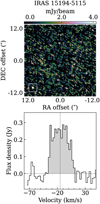 |
Fig. C.76 C13CCCH, N=11-10, J=23/2-21/2 (104.13854 GHz) |
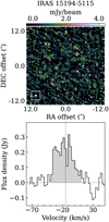 |
Fig. C.77 C13CCCH, N=11-10, J=21/2-19/2 (104.17622 GHz) |
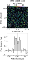 |
Fig. C.78 CC13CCH, N=11-10, J=23/2-21/2 (104.29734 GHz) |
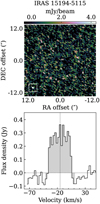 |
Fig. C.79 CC13CCH, N=11-10, J=21/2-19/2 (104.33572 GHz) |
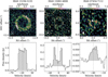 |
Fig. C.80 C4H, N=11-10, J=23/2-21/2 (104.666566 GHz) |
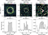 |
Fig. C.81 C4H, N=11-10, J=21/2-19/2 (104.70511 GHz) |
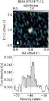 |
Fig. C.82 30SiS, 6-5 (105.059203 GHz) |
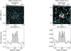 |
Fig. C.83 H13CCCN, 12-11 (105.799113 GHz) |
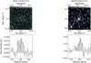 |
Fig. C.84 Si34S, 6-5 (105.941503 GHz) |
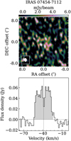 |
Fig. C.85 CCS, 89-78 (106.347726 GHz) |
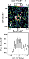 |
Fig. C.86 HC5N, 40-39 (106.49891 GHz) |
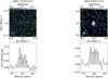 |
Fig. C.87 29SiS, 6-5 (106.92298 GHz) |
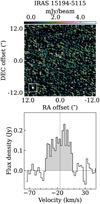 |
Fig. C.88 Si13CC, 51,5-41,4 (107.971477 GHz) |
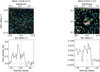 |
Fig. C.89 HC13CCN, 12-11 (108.710532 GHz) |
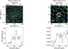 |
Fig. C.90 HCC13CN, 12-11 (108.720999 GHz) |
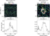 |
Fig. C.91 13CN, N=1-0, J=3/2-1/2 (108.782374 GHz) |
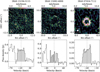 |
Fig. C.92 C3N, 11-10 (A) (108.83425 GHz) |
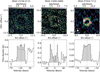 |
Fig. C.93 C3N, 11-10 (B) (108.853 GHz) |
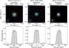 |
Fig. C.94 SiS, 6-5 (108.924301 GHz) |
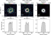 |
Fig. C.95 HC3N, 12-11 (109.173634 GHz) |
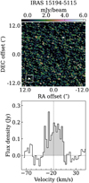 |
Fig. C.96 CCC13CH, N=12-11, J=25/2-23/2 (110.735027 GHz) |
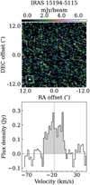 |
Fig. C.97 CCC13CH, N=12-11, J=23/2-21/2 (110.772434 GHz) |
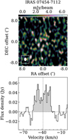 |
Fig. C.98 HC5N, 42-41 (111.823024 GHz) |
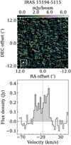 |
Fig. C.99 Si13CC, 50,5-40,4 (112.593212 GHz) |
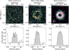 |
Fig. C.100 CN, N=1-0, J=1/2-1/2, F=1/2-3/2 (113.144157 GHz) |
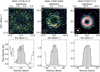 |
Fig. C.101 CN, N=1-0, J=1/2-1/2, F=3/2-1/2 (113.170492 GHz) |
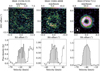 |
Fig. C.102 CN, N=1-0, J=1/2-1/2, F=3/2-3/2 (113.191279 GHz) |
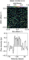 |
Fig. C.103 C13CCCH, N=12-11, J=23/2-21/2 (113.6442 GHz) |
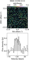 |
Fig. C.104 CC13CCH, N=12-11, J=23/2-21/2 (113.81808 GHz) |
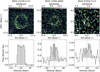 |
Fig. C.105 C4H, N=12-11, J=25/2-23/2 (114.182514 GHz) |
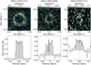 |
Fig. C.106 C4H, N=12-11, J=23/2-21/2 (114.221042 GHz) |
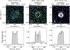 |
Fig. C.107 SiC2, 50,5-40,4 (115.382389 GHz) |
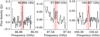 |
Fig. C.108 Spectra of unidentified lines towards IRAS 15194-5115. The width of the region shaded in pink is twice the expansion velocity of the source CSE. The feature to the left of the 87.59 GHz line is a blend of the 30SiS 5−4 and SiN 2−1 lines. The u-lines are too weak to show any structure in the emission maps. They are not detected in the other two sources. |
The below figures show the spectra of the lines from the APEX surveys that we have used in this work, for IRAS 15194−5115 (left), IRAS 15082−4808 (centre), and IRAS 07454−7112 (right). The figures are ordered in increasing order of line rest frequency, which is given in parentheses at the end of the figure caption. Missing plots indicate non-detection of the concerned line towards the particular source. The dotted vertical line marks the systemic velocity of the source. The grey shaded regions cover 1.2 times the expansion velocity on either side of the systemic velocity. For non-blended lines, this region represents the channels used for calculating the integrated line intensities, reported in Table B.2. For the lines of C3N (Figs. C.113, C.147, C.158, C.165, C.183), where the line profile consists of blended hyperfine components, the whole line profile, not just the grey shaded region, has been integrated to obtain the integrated line intensity. For lines of C2H and C4H, which have hyperfine components, we have shown only the strongest or unblended component, but the total integrated intensity was calculated by summing up all the components per transition.
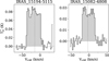 |
Fig. C.109 C4H, N=17-16 (161.796566 GHz) |
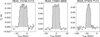 |
Fig. C.110 SiS, 9-8 (163.376785 GHz) |
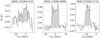 |
Fig. C.111 HC3N, J=18-17 (163.753389 GHz) |
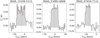 |
Fig. C.112 SiC2, 7( 2, 6)- 6( 2, 5) (164.069091 GHz) |
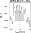 |
Fig. C.113 C3N N=17-16 (168.2043 GHz). |
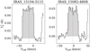 |
Fig. C.114 C4H, N=18-17 (171.310707 GHz) |
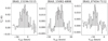 |
Fig. C.115 29SiO, 4-3 (171.512796 GHz) |
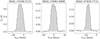 |
Fig. C.116 H13CN, J=2-1 (172.677851 GHz) |
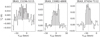 |
Fig. C.117 HC3N, J=19-18 (172.8493 GHz) |
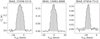 |
Fig. C.118 SiO, 4-3 (173.688238 GHz) |
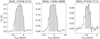 |
Fig. C.119 C2H, N=2-1 (174.663199 GHz) |
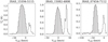 |
Fig. C.120 HCN, J=2-1 (177.261111 GHz) |
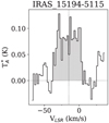 |
Fig. C.121 C4H, N=19-18 (180.824472 GHz) |
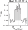 |
Fig. C.122 HNC, J=2-1 (181.324758 GHz) |
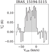 |
Fig. C.123 SiS, 10-9 (181.525218 GHz) |
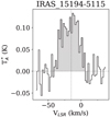 |
Fig. C.124 13CS, J=4-3 (184.981772 GHz) |
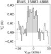 |
Fig. C.125 SiC2, 8( 6, 3)- 7( 6, 2) (188.3857 GHz) |
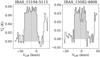 |
Fig. C.126 C4H N=20-19 (190.337804 GHz) |
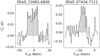 |
Fig. C.127 HC3N, J=21-20 (191.040299 GHz) |
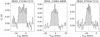 |
Fig. C.128 C34S, 4-3 (192.818457 GHz) |
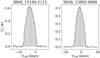 |
Fig. C.129 CS, 4-3 (195.954211 GHz) |
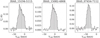 |
Fig. C.130 SiS, 11-10 (199.672229 GHz) |
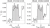 |
Fig. C.131 C4H N=21-20 (199.850787 GHz) |
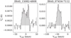 |
Fig. C.132 HC3N, J=23-22 (209.230234 GHz) |
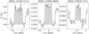 |
Fig. C.133 C4H, N=22-21 (209.363302 GHz) |
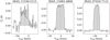 |
Fig. C.134 SiC2, 9( 2, 8)- 8( 2, 7) (209.892001 GHz) |
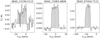 |
Fig. C.135 SiC2, 9( 6, 4)- 8( 6, 3) (212.031878 GHz) |
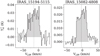 |
Fig. C.136 SiC2, 9( 4, 6)- 8( 4, 5) (213.208032 GHz) |
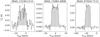 |
Fig. C.137 SiC2, 9( 4, 5)- 8( 4, 4) (213.292337 GHz) |
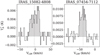 |
Fig. C.138 29SiS, 12-11 (213.81614 GHz) |
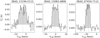 |
Fig. C.139 29SiO, 5-4 (214.385752 GHz) |
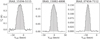 |
Fig. C.140 SiO, 5-4 (217.104919 GHz) |
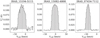 |
Fig. C.141 SiS, 12-11 (217.817663 GHz) |
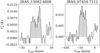 |
Fig. C.142 HC3N, J=24-23 (218.324723 GHz) |
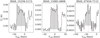 |
Fig. C.143 C4H N=23-22 (218.875369 GHz) |
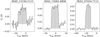 |
Fig. C.144 SiC2, 10( 0,10)- 9( 0, 9) (220.773685 GHz) |
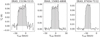 |
Fig. C.145 SiC2, 9( 2, 7)- 8( 2, 6) (222.009386 GHz) |
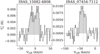 |
Fig. C.146 HC3N J=25-24 (227.418905 GHz) |
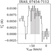 |
Fig. C.147 C3N, N=23-22 (227.5539 GHz) |
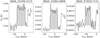 |
Fig. C.148 C4H, N=24-23 (228.386962 GHz) |
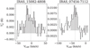 |
Fig. C.149 Si34S, 13-12 (229.500868 GHz) |
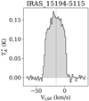 |
Fig. C.150 13CS, J=5-4 (231.220685 GHz) |
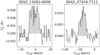 |
Fig. C.151 29SiS, 13-12 (231.626673 GHz) |
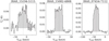 |
Fig. C.152 SiC2, 10( 2, 9)- 9( 2, 8) (232.53407 GHz) |
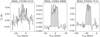 |
Fig. C.153 SiC2, 10( 6, 5)- 9( 6, 4) (235.712998 GHz) |
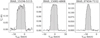 |
Fig. C.154 SiS, 13-12 (235.961363 GHz) |
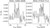 |
Fig. C.155 HC3N, J=26-27 (236.512789 GHz) |
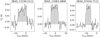 |
Fig. C.156 SiC2, 10( 4, 7)- 9( 4, 6) (237.150018 GHz) |
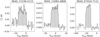 |
Fig. C.157 SiC2, 10( 4, 6)- 9( 4, 5) (237.331309 GHz) |
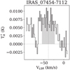 |
Fig. C.158 C3N, N=24-23 (237.44415 GHz) |
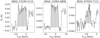 |
Fig. C.159 C4H, N=25-24 (237.89806 GHz) |
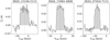 |
Fig. C.160 C34S, 5-4 (241.016089 GHz) |
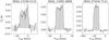 |
Fig. C.161 SiC2, 11( 0,11)-10( 0,10) (241.367708 GHz) |
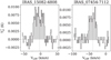 |
Fig. C.162 C33S, 5-4 (242.91361 GHz) |
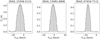 |
Fig. C.163 CS, 5-4 (244.935556 GHz) |
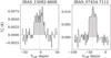 |
Fig. C.164 Si34S, 14-13 (247.146242 GHz) |
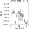 |
Fig. C.165 C3N, N=25-24 (247.334 GHz) |
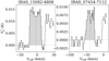 |
Fig. C.166 C4H, N=26-25 (247.408643 GHz) |
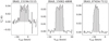 |
Fig. C.167 SiC2, 10( 2, 8)- 9( 2, 7) (247.52912 GHz) |
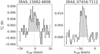 |
Fig. C.168 29SiS, 14-13 (249.435412 GHz) |
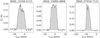 |
Fig. C.169 SiS, 14-13 (254.103211 GHz) |
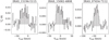 |
Fig. C.170 30SiO, 6-5 (254.216656 GHz) |
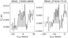 |
Fig. C.171 C4H, N=27-26 (256.918691 GHz) |
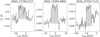 |
Fig. C.172 29SiO, 6-5 (257.255213 GHz) |
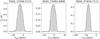 |
Fig. C.173 H13CN, J=3-2 (259.011798 GHz) |
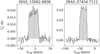 |
Fig. C.174 SiC2, 11( 6, 6)-10( 6, 5) (259.433309 GHz) |
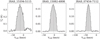 |
Fig. C.175 SiO, 6-5 (260.518009 GHz) |
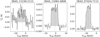 |
Fig. C.176 SiC2, 11( 4, 8)-10( 4, 7) (261.150695 GHz) |
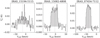 |
Fig. C.177 SiC2, 11( 4, 7)-10( 4, 6) (261.509329 GHz) |
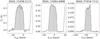 |
Fig. C.178 C2H, N=3-2 (262.064986 GHz) |
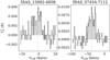 |
Fig. C.179 30SiS, 15-14 (262.585033 GHz) |
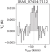 |
Fig. C.180 Si34S, 15-14 (264.789719 GHz) |
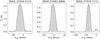 |
Fig. C.181 HCN, J=3-2 (265.886434 GHz) |
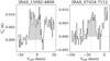 |
Fig. C.182 C4H, N=28-27 (266.428184 GHz) |
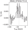 |
Fig. C.183 C3N, N=27-26 (267.11225 GHz) |
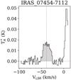 |
Fig. C.184 29SiS, 15-14 (267.242218 GHz) |
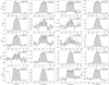 |
Fig. C.185 Lines from the APEX Band 7 (272–376 GHz) survey of IRAS 15194-5115, which have been used in this work. The grey shaded regions represent the channels used for calculating the integrated intensities of the lines, reported in Table B.2. The dotted vertical line marks the systemic velocity of the source. |
Appendix D AzimuthaMy-averaged radial profiles (AARPs)
The figures below show the Gaussian fits to the AARPs of the systemic velocity emission maps of the 14 species shown in Fig. 9. The details of these profiles and fits are explained in Sect. 4.3.2.
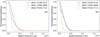 |
Fig. D.1 AARPs (solid) and Gaussian fits (dashed) for SiO (left) and SiS (right) emission. |
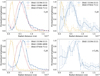 |
Fig. D.4 Same as Fig. D.1 but for C2H (top left), C3H (top right), C4H (bottom left), and c-C3H2 (bottom right) emission |
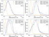 |
Fig. D.5 Same as Fig. D.1 but for HC3N (top left), C3N (top right), HC5N (bottom left), and HNC (bottom right) emission |
Appendix E Column densities and abundances: Methods
The results in this section are based on a simple model for the CSE, assuming an isotropic, constant mass-loss rate and gas expanding at its terminal velocity. Nevertheless, there are clear indications of deviations from such a simple model, particularly in terms of the morphology, as is discussed in Sect. 4.3.1.
We express molecular abundances as fractional abundances relative to that of molecular hydrogen, H2, which has the abundance distribution with the largest spatial extent (Huggins & Glassgold 1982). The fractional abundance profile of a molecular species, X, is defined as
 (E.1)
(E.1)
where nX(r) and  are the number density distributions of the molecule and molecular hydrogen, respectively.
The excitation of a molecule in the CSE is determined by collisions and radiation, in particular the radiation fields of the central star and circumstellar dust. Non-local thermodynamic equilibrium (non-LTE) conditions can be prevalent in CSEs, which calls for a detailed radiative transfer analysis for the proper treatment of molecular excitation. Such a non-LTE treatment is outside the scope of the current work, and will be presented in an upcoming paper. A simpler analysis assuming LTE conditions can provide reasonable estimates of the molecular abundances and offer substantial insights into circumstellar chemistry, and is regularly employed as a first tool to analyse spectral surveys and other large datasets of evolved stars (e.g. Cernicharo et al. 2000; Justtanont et al. 2000; Wesson et al. 2010; Patel et al. 2011; Sanchez Contreras et al. 2015; Smith et al. 2015; Velilla Prieto et al. 2015b; Pardo et al. 2022). For molecules with multiple rotational transitions detected, the rotational temperature and column density can be estimated using a population diagram (Sect. E.1). The column densities thus obtained, together with the emission region sizes calculated from the AARPs, can be used to estimate molecular fractional abundances. In those cases where the population diagram method can not be employed, owing to the lack of a sufficient number of transitions covering a broad range of upper-level energies, we performed an approximate calculation of the fractional abundance using a single line for each species (Sect. E.3). We describe both methods below.
Appendix E.1 The population diagram method
The column density of each rotational energy level is related to the rotational temperature, Trot, and total column density, Ntot, by the relation
 (E.2)
(E.2)
where Nu is the column density of molecules in the upper energy level having energy Eu and statistical weight gu, and Z and kB are the partition function and the Boltzmann constant, respectively (Goldsmith & Langer 1999). For the calculation of partition functions, all molecules used for producing population diagrams (see Table 6) have been regarded as linear rigid rotors, except SiC2 and c-C3H2, which are asymmetric tops. In order to use the integrated intensities summed over the hyperfine components wherever present (e.g. C2H, C3N), we calculated the partition functions, degeneracy factors, and Einstein A-coefficients under the assumption that the molecules do not possess a hyperfine structure. For the asymmetric tops, we interpolated the partition function values from the CDMS (Müller et al. 2005) catalogue to the rotation temperatures obtained from our analysis.
The source-averaged column density of the upper state, Nu, can be calculated from the observed velocity-integrated flux, ∫Suldv, of the corresponding rotational emission line as
 (E.3)
(E.3)
where vul is the rest frequency of the transition, Aul is the Einstein A-coefficient, Ωs is the solid angle of the emitting region, h is the Planck constant, c is the speed of light in vacuum, and  is the optical depth correction factor (see Goldsmith & Langer 1999), given by
 (E.4)
(E.4)
where τν is the optical depth of the line.
If the assumptions are correct that, firstly, the populations of the corresponding energy levels follow a Boltzmann distribution that can be described by a single excitation temperature, Trot, and, secondly, the lines are optically thin, then the points in the plot of ln(Nu/gu) versus Eu/kB are expected to lie on a straight line (see e.g. Fig. E.1). The rotational temperature and column density of each molecule are calculated from the slope and intercept, respectively, of a linear fit to such a plot.
Using this method, we first obtained estimates of the rotational temperature and total column density for each species without an optical depth correction ( ). From these values, we then calculated a preliminary estimate of the optical depth for each individual line of the species, using the standard equation
 (E.5)
(E.5)
where Δυ is the full velocity width of the line. The range of optical depths thus calculated for each species for the three stars are given in Table E.1.
Employing the correction factors (see Eq. E.4) obtained from the calculated optical depths, we then produced optical-depth-corrected population diagrams, from which optical-depth-corrected rotation temperatures and total column densities were estimated. These values are presented in Table 6. The optical-depth-corrected population diagrams are shown in Figs. E.1 - E.18.
We note that along with the lines from the ALMA data, we have also included lines detected in our APEX surveys (Table B.2 and Figs. C.109–C.185) in the population diagrams, so that a wider range of energy levels can be sampled.
Appendix E.2 Abundance calculation from column densities
Using the estimates of the radial extents of the emitting regions of different species obtained from the Gaussian fits to the AARPs (see Sect. 4.3.2), we can estimate the molecular fractional abundances (Table 7) from the column densities of the respective species given by the population diagrams, using the equation
 (E.6)
(E.6)
where Ṁ is the hydrogen mass-loss rate, υexp the gas expansion velocity, and mH the mass of the hydrogen atom, and where Ri and Re are the inner and outer radii of the emitting region, respectively (Olofsson 2003).
Range of optical depths per molecule
Appendix E.3 Abundance calculation from single lines
Population diagrams cannot be used in the case of molecules for which only one or two lines are detected, or for which the detected transitions are very close together in upper-level energies. In such cases, we obtained a rough estimate of the fractional abundance, using the highest signal-to-noise line available, by assuming it to be constant in the radial range Ri to Re and zero outside it. Assuming an r−2 density distribution and a constant, assumed excitation temperature throughout the emitting region, we used the following formula from Habing & Olofsson (2004, in rewritten form)
 (E.7)
(E.7)
where υexp is given in km/s, Ṁ in M⊙ yr−1, D in kpc, Ri and Re in cm, and ∫S uldv in Jykm/s. The assumed Tex values are 40 K for centrally peaked species and 20 K for shell species (see Sect. 4.4 for a justification of these values). We note that we did not perform optical depth corrections in the case of singleline abundance estimates, as the temperature we used for these calculations was an assumed value, and since the high uncertainties involved anyway deem the abundances thus calculated to be order of magnitude estimates.
The figures below show the population diagrams (see Sect. E.1) of various molecular species (listed in Table 6) towards the three stars.
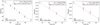 |
Fig. E.1 Population diagrams for SiO for the three stars, IRAS 15194–5115 (left), IRAS 15082–4808 (centre), and IRAS 07454–7112 (right). The solid line (red) is the best-fit linear model to the data (black). Rotation temperatures, Trot, and source-averaged column densities, Ntot, are listed in the legends. Circle and square points denote lines observed with ALMA and APEX, respectively. Hollow circles denote lines for which data combination (see Sect. 3.3) was performed. |
References
- Abia, C., Busso, M., Gallino, R., et al. 2001, ApJ, 559, 1117 [Google Scholar]
- Agundez, M. 2009, PhD thesis, Center for Astrobiology, Madrid, Spain [Google Scholar]
- Agúndez, M. 2022, Eur. Phys. J. Conf., 265, 00029 [CrossRef] [EDP Sciences] [Google Scholar]
- Agúndez, M., Fonfria, J. P., Cernicharo, J., et al. 2012, A&A, 543, A48 [NASA ADS] [CrossRef] [EDP Sciences] [Google Scholar]
- Agúndez, M., Cernicharo, J., Quintana-Lacaci, G., et al. 2017, A&A, 601, A44 [NASA ADS] [CrossRef] [EDP Sciences] [Google Scholar]
- Agúndez, M., Martinez, J. I., de Andres, P. L., Cernicharo, J., & Martin-Gago, J. A. 2020, A&A, 637, A59 [CrossRef] [EDP Sciences] [PubMed] [Google Scholar]
- Allain, T., Sedlmayr, E., & Leach, S. 1997, A&A, 323, 163 [Google Scholar]
- Andriantsaralaza, M., Ramstedt, S., Vlemmings, W. H. T., & De Beck, E. 2022, A&A, 667, A74 [NASA ADS] [CrossRef] [EDP Sciences] [Google Scholar]
- Asplund, M., Grevesse, N., Sauval, A. J., & Scott, P. 2009, ARA & A, 47, 481 [NASA ADS] [CrossRef] [Google Scholar]
- Belitsky, V., Lapkin, I., Fredrixon, M., et al. 2018, A&A, 612, A23 [NASA ADS] [CrossRef] [EDP Sciences] [Google Scholar]
- Billade, B., Nystrom, O., Meledin, D., et al. 2012, IEEE Transac. Terahertz Sci. Technol., 2, 208 [CrossRef] [Google Scholar]
- Butler, B. 2012, Atacama Large Millimeter/Submillimeter Array Memo, 594, 1 [NASA ADS] [Google Scholar]
- Canosa, A., Le Picard, S. D., Gougeon, S., et al. 2001, J. Chem. Phys., 115, 6495 [NASA ADS] [CrossRef] [Google Scholar]
- Cernicharo, J., Guélin, M., & Kahane, C. 2000, A&AS, 142, 181 [NASA ADS] [CrossRef] [EDP Sciences] [Google Scholar]
- Cernicharo, J., Waters, L. B. F. M., Decin, L., et al. 2010, A&A, 521, L8 [NASA ADS] [CrossRef] [EDP Sciences] [Google Scholar]
- Cernicharo, J., Daniel, F., Castro-Carrizo, A., et al. 2013, ApJ, 778, L25 [CrossRef] [Google Scholar]
- Cernicharo, J., Teyssier, D., Quintana-Lacaci, G., et al. 2014, ApJ, 796, L21 [NASA ADS] [CrossRef] [Google Scholar]
- Cernicharo, J., Marcelino, N., Agúndez, M., & Guélin, M. 2015, A&A, 575, A91 [NASA ADS] [CrossRef] [EDP Sciences] [Google Scholar]
- Cernicharo, J., Cabezas, C., Pardo, J. R., et al. 2023a, A&A, 672, L13 [NASA ADS] [CrossRef] [EDP Sciences] [Google Scholar]
- Cernicharo, J., Pardo, J. R., Cabezas, C., et al. 2023b, A&A, 670, L19 [NASA ADS] [CrossRef] [EDP Sciences] [Google Scholar]
- Cherchneff, I., Barker, J. R., & Tielens, A. G. G. M. 1992, ApJ, 401, 269 [Google Scholar]
- Claude, S., Dindo, P., Erickson, D., et al. 2005, in The Joint 30th International Conference on Infrared and Millimeter Waves and 13th International Conference on Terahertz Electronics, 407 [Google Scholar]
- Cordiner, M. A., & Millar, T. J. 2009, ApJ, 697, 68 [NASA ADS] [CrossRef] [Google Scholar]
- Cornwell, T. J. 2008, IEEE J. Selected Topics in Signal Process., 2, 793 [NASA ADS] [CrossRef] [Google Scholar]
- Daniel, F., Agúndez, M., Cernicharo, J., et al. 2012, A&A, 542, A37 [NASA ADS] [CrossRef] [EDP Sciences] [Google Scholar]
- De Beck, E., Lombaert, R., Agúndez, M., et al. 2012, A&A, 539, A108 [NASA ADS] [CrossRef] [EDP Sciences] [Google Scholar]
- Decin, L., Richards, A. M. S., Neufeld, D., et al. 2015, A&A, 574, A5 [NASA ADS] [CrossRef] [EDP Sciences] [Google Scholar]
- Di Criscienzo, M., Ventura, P., García-Hernández, D. A., et al. 2016, MNRAS, 462, 395 [NASA ADS] [CrossRef] [Google Scholar]
- Dinh-V-Trung, & Lim, J. 2008, ApJ, 678, 303 [Google Scholar]
- Feast, M. W., Whitelock, P. A., & Marang, F. 2003, MNRAS, 346, 878 [NASA ADS] [CrossRef] [Google Scholar]
- Fonfria, J. P., Fernández-López, M., Agúndez, M., et al. 2014, MNRAS, 445, 3289 [NASA ADS] [CrossRef] [Google Scholar]
- Fonfria, J. P., Fernández-López, M., Pardo, J. R., et al. 2018, ApJ, 860, 162 [CrossRef] [Google Scholar]
- Goddi, C., Martí-Vidal, I., Messias, H., et al. 2019, PASP, 131, 075003 [Google Scholar]
- Goldsmith, P. F., & Langer, W. D. 1999, ApJ, 517, 209 [Google Scholar]
- Gong, Y., Henkel, C., Spezzano, S., et al. 2015, A&A, 574, A56 [NASA ADS] [CrossRef] [EDP Sciences] [Google Scholar]
- Groenewegen, M. A. T. 1997, A&A, 317, 503 [NASA ADS] [Google Scholar]
- Groenewegen, M. A. T., Whitelock, P. A., Smith, C. H., & Kerschbaum, F. 1998, MNRAS, 293, 18 [NASA ADS] [CrossRef] [Google Scholar]
- Groenewegen, M. A. T., Barlow, M. J., Blommaert, J. A. D. L., et al. 2012, A&A, 543, L8 [NASA ADS] [CrossRef] [EDP Sciences] [Google Scholar]
- Guélin, M., Patel, N. A., Bremer, M., et al. 2018, A&A, 610, A4 [NASA ADS] [CrossRef] [EDP Sciences] [Google Scholar]
- Guilloteau, S., Omont, A., & Lucas, R. 1987, A&A, 176, L24 [NASA ADS] [Google Scholar]
- Güsten, R., Nyman, L. Å., Schilke, P., et al. 2006, A&A, 454, L13 [NASA ADS] [CrossRef] [EDP Sciences] [Google Scholar]
- Guzmán, A. E., Verdugo, C., Nagai, H., et al. 2019, PASP, 131, 094504 [CrossRef] [Google Scholar]
- Habing, H. J., & Olofsson, H. 2004, Asymptotic Giant Branch Stars (Berlin: Springer) [CrossRef] [Google Scholar]
- Harada, N., Herbst, E., & Wakelam, V. 2010, ApJ, 721, 1570 [NASA ADS] [CrossRef] [Google Scholar]
- He, J. H., Dinh-V-Trung, Kwok, S., et al. 2008, ApJS, 177, 275 [NASA ADS] [CrossRef] [Google Scholar]
- He, J. H., Kamiński, T., Mennickent, R. E., et al. 2019, ApJ, 883, 165 [NASA ADS] [CrossRef] [Google Scholar]
- Henry, R. B. C., Speck, A., Karakas, A. I., Ferland, G. J., & Maguire, M. 2012, ApJ, 749, 61 [NASA ADS] [CrossRef] [Google Scholar]
- Herbst, E., & Leung, C. M. 1990, A&A, 233, 177 [NASA ADS] [Google Scholar]
- Herwig, F. 2005, ARA & A, 43, 435 [NASA ADS] [CrossRef] [Google Scholar]
- Höfner, S. 2008, A&A, 491, L1 [NASA ADS] [CrossRef] [EDP Sciences] [Google Scholar]
- Höfner, S. 2015, ASP Conf. Ser., 497, 333 [Google Scholar]
- Höfner, S., & Olofsson, H. 2018, A & A Rev., 26, 1 [Google Scholar]
- Howe, D. A., & Millar, T. J. 1990, MNRAS, 244, 444 [NASA ADS] [Google Scholar]
- Huggins, P. J., & Glassgold, A. E. 1982, ApJ, 252, 201 [NASA ADS] [CrossRef] [Google Scholar]
- Humire, P. K., Thiel, V., Henkel, C., et al. 2020, A&A, 642, A222 [NASA ADS] [CrossRef] [EDP Sciences] [Google Scholar]
- Izzard, R. G., & Tout, C. A. 2003, PASA, 20, 345 [NASA ADS] [CrossRef] [Google Scholar]
- Jeste, M., Gong, Y., Wong, K. T., et al. 2022, A&A, 666, A69 [NASA ADS] [CrossRef] [EDP Sciences] [Google Scholar]
- Jolly, J.-B., Knudsen, K. K., & Stanley, F. 2020, MNRAS, 499, 3992 [Google Scholar]
- Justtanont, K., Barlow, M. J., Tielens, A. G. G. M., et al. 2000, A&A, 360, 1117 [NASA ADS] [Google Scholar]
- Kahane, C., Gomez-Gonzalez, J., Cernicharo, J., & Guelin, M. 1988, A&A, 190, 167 [NASA ADS] [Google Scholar]
- Karakas, A. I., & Lugaro, M. 2016, ApJ, 825, 26 [NASA ADS] [CrossRef] [Google Scholar]
- Kepley, A. A., Tsutsumi, T., Brogan, C. L., et al. 2020, PASP, 132, 024505 [Google Scholar]
- Kraemer, K. E., Sloan, G. C., Keller, L. D., et al. 2019, ApJ, 887, 82 [NASA ADS] [CrossRef] [Google Scholar]
- Lambert, D. L., Gustafsson, B., Eriksson, K., & Hinkle, K. H. 1986, ApJS, 62, 373 [Google Scholar]
- Lattanzio, J. C., & Boothroyd, A. I. 1997, AIP Conf. Ser., 402, 85 [NASA ADS] [Google Scholar]
- Lattanzio, J. C., Frost, C. A., Cannon, R. C., & Wood, P. R. 1997, Nuclear Physics A, 621, 435 [Google Scholar]
- Leão, I. C., de Laverny, P., Mékarnia, D., de Medeiros, J. R., & Vandame, B. 2006, A&A, 455, 187 [NASA ADS] [CrossRef] [EDP Sciences] [Google Scholar]
- Li, X., Millar, T. J., Walsh, C., Heays, A. N., & van Dishoeck, E. F. 2014, A&A, 568, A111 [NASA ADS] [CrossRef] [EDP Sciences] [Google Scholar]
- Lucas, R., Guélin, M., Kahane, C., Audinos, P., & Cernicharo, J. 1995, Ap & SS, 224, 293 [NASA ADS] [CrossRef] [Google Scholar]
- Lykou, F., Zijlstra, A. A., Kluska, J., et al. 2018, MNRAS, 480, 1006 [NASA ADS] [CrossRef] [Google Scholar]
- MacKay, D. D. S., & Charnley, S. B. 1999, MNRAS, 302, 793 [NASA ADS] [CrossRef] [Google Scholar]
- Maret, S., Hily-Blant, P., Pety, J., Bardeau, S., & Reynier, E. 2011, A&A, 526, A47 [NASA ADS] [CrossRef] [EDP Sciences] [Google Scholar]
- Massalkhi, S., Agúndez, M., Cernicharo, J., et al. 2018, A&A, 611, A29 [CrossRef] [EDP Sciences] [PubMed] [Google Scholar]
- Massalkhi, S., Agúndez, M., & Cernicharo, J. 2019, A&A, 628, A62 [CrossRef] [EDP Sciences] [PubMed] [Google Scholar]
- Matsuura, M., Barlow, M. J., Zijlstra, A. A., et al. 2009, MNRAS, 396, 918 [NASA ADS] [CrossRef] [Google Scholar]
- Mauron, N., & Huggins, P. J. 1999, A&A, 349, 203 [NASA ADS] [Google Scholar]
- Mauron, N., & Huggins, P. J. 2000, A&A, 359, 707 [Google Scholar]
- McGuire, B. A. 2022, ApJS, 259, 30 [NASA ADS] [CrossRef] [Google Scholar]
- McMullin, J. P., Waters, B., Schiebel, D., Young, W., & Golap, K. 2007, ASP Conf. Ser., 376, 127 [Google Scholar]
- Menten, K. M., Reid, M. J., Kamiński, T., & Claussen, M. J. 2012, A&A, 543, A73 [NASA ADS] [CrossRef] [EDP Sciences] [Google Scholar]
- Menten, K. M., Wyrowski, F., Keller, D., & Kamiński, T. 2018, A&A, 613, A49 [NASA ADS] [CrossRef] [EDP Sciences] [Google Scholar]
- Millar, T. J., & Herbst, E. 1994, A&A, 288, 561 [NASA ADS] [Google Scholar]
- Müller, H. S., Schlöder, F., Stutzki, J., & Winnewisser, G. 2005, J. Mol. Struc., 742, 215 [CrossRef] [Google Scholar]
- Nyman, L. A., Olofsson, H., Johansson, L. E. B., et al. 1993, A&A, 269, 377 [NASA ADS] [Google Scholar]
- Olofsson, H. 2003, in Asymptotic Giant Branch Stars (Berlin: Springer), 325 [Google Scholar]
- Pardo, J. R., Cernicharo, J., Velilla Prieto, L., et al. 2018, A&A, 615, L4 [NASA ADS] [CrossRef] [EDP Sciences] [Google Scholar]
- Pardo, J. R., Cernicharo, J., Tercero, B., et al. 2022, A&A, 658, A39 [NASA ADS] [CrossRef] [EDP Sciences] [Google Scholar]
- Patel, N. A., Young, K. H., Gottlieb, C. A., et al. 2011, ApJS, 193, 17 [NASA ADS] [CrossRef] [Google Scholar]
- Ramstedt, S., & Olofsson, H. 2014, A&A, 566, A145 [NASA ADS] [CrossRef] [EDP Sciences] [Google Scholar]
- Rau, U., & Cornwell, T. J. 2011, A&A, 532, A71 [NASA ADS] [CrossRef] [EDP Sciences] [Google Scholar]
- Remijan, A. J., Markwick-Kemper, A., & ALMA Working Group on Spectral Line Frequencies 2007, AAS Meeting Abstracts, 211, 132.11 [Google Scholar]
- Saberi, M., Vlemmings, W. H. T., & De Beck, E. 2019, A&A, 625, A81 [NASA ADS] [CrossRef] [EDP Sciences] [Google Scholar]
- Saberi, M., Olofsson, H., Vlemmings, W. H. T., et al. 2020, A&A, 638, A99 [NASA ADS] [CrossRef] [EDP Sciences] [Google Scholar]
- Sanchez Contreras, C., Velilla Prieto, L., Agúndez, M., et al. 2015, A&A, 577, A52 [NASA ADS] [CrossRef] [EDP Sciences] [Google Scholar]
- Sarre, P. J., Hurst, M. E., & Lloyd Evans, T. 1996, ApJ, 471, L107 [NASA ADS] [CrossRef] [Google Scholar]
- Schöier, F. L., Olofsson, H., & Lundgren, A. A. 2006, A&A, 454, 247 [NASA ADS] [CrossRef] [EDP Sciences] [Google Scholar]
- Schöier, F. L., Bast, J., Olofsson, H., & Lindqvist, M. 2007, A&A, 473, 871 [NASA ADS] [CrossRef] [EDP Sciences] [Google Scholar]
- Schöier, F. L., Ramstedt, S., Olofsson, H., et al. 2013, A&A, 550, A78 [Google Scholar]
- Shingles, L. J., & Karakas, A. I. 2013, MNRAS, 431, 2861 [NASA ADS] [CrossRef] [Google Scholar]
- Siebert, M. A., Van de Sande, M., Millar, T. J., & Remijan, A. J. 2022, ApJ, 941, 90 [NASA ADS] [CrossRef] [Google Scholar]
- Sloan, G. C., Little-Marenin, I. R., & Price, S. D. 1998, AJ, 115, 809 [NASA ADS] [CrossRef] [Google Scholar]
- Smith, C. L., Zijlstra, A. A., & Fuller, G. A. 2014, MNRAS, 440, 172 [NASA ADS] [CrossRef] [Google Scholar]
- Smith, C. L., Zijlstra, A. A., & Fuller, G. A. 2015, MNRAS, 454, 177 [NASA ADS] [CrossRef] [Google Scholar]
- Tenenbaum, E. D., Dodd, J. L., Milam, S. N., Woolf, N. J., & Ziurys, L. M. 2010, ApJS, 190, 348 [NASA ADS] [CrossRef] [Google Scholar]
- Tielens, A. G. G. M. 2005, The Physics and Chemistry of the Interstellar Medium (Cambridge: Cambridge University Press) [Google Scholar]
- Van de Sande, M., & Millar, T. J. 2022, MNRAS, 510, 1204 [Google Scholar]
- Van de Sande, M., Sundqvist, J. O., Millar, T. J., et al. 2018, A&A, 616, A106 [NASA ADS] [CrossRef] [EDP Sciences] [Google Scholar]
- Van de Sande, M., Sundqvist, J. O., Millar, T. J., Keller, D., & Decin, L. 2019, IAU Symp., 343, 531 [NASA ADS] [Google Scholar]
- van Dishoeck, E. F. 1988, Astrophys. Space Sci. Lib., 146, 49 [NASA ADS] [CrossRef] [Google Scholar]
- Vassilev, V., Meledin, D., Lapkin, I., et al. 2008, A&A, 490, 1157 [NASA ADS] [CrossRef] [EDP Sciences] [Google Scholar]
- Vassiliadis, E., & Wood, P. R. 1993, ApJ, 413, 641 [Google Scholar]
- Velilla Prieto, L., Cernicharo, J., Quintana-Lacaci, G., et al. 2015a, ApJ, 805, L13 [NASA ADS] [CrossRef] [Google Scholar]
- Velilla Prieto, L., Sánchez Contreras, C., Cernicharo, J., et al. 2015b, A&A, 575, A84 [CrossRef] [EDP Sciences] [Google Scholar]
- Velilla-Prieto, L., Cernicharo, J., Agúndez, M., et al. 2019, A&A, 629, A146 [NASA ADS] [CrossRef] [EDP Sciences] [Google Scholar]
- Vlemmings, W. H. T., Maercker, M., Lindqvist, M., et al. 2013, A&A, 556, L1 [NASA ADS] [CrossRef] [EDP Sciences] [Google Scholar]
- Wesson, R., Cernicharo, J., Barlow, M. J., et al. 2010, A&A, 518, L144 [NASA ADS] [CrossRef] [EDP Sciences] [Google Scholar]
- Whitelock, P. A., Feast, M. W., Marang, F., & Groenewegen, M. A. T. 2006, MNRAS, 369, 751 [NASA ADS] [CrossRef] [Google Scholar]
- Woods, P. M., Schöier, F. L., Nyman, L. Å., & Olofsson, H. 2003, A&A, 402, 617 [NASA ADS] [CrossRef] [EDP Sciences] [Google Scholar]
- Yasuda, Y., & Kozasa, T. 2012, ApJ, 745, 159 [NASA ADS] [CrossRef] [Google Scholar]
- Zijlstra, A. A., Matsuura, M., Wood, P. R., et al. 2006, MNRAS, 370, 1961 [Google Scholar]
See the ALMA Technical Handbook, https://almascience.eso.org/proposing/technical-handbook
All Tables
All Figures
|
Fig. 1 CS .J = 2−1 emission at 97.98 GHz towards IRAS 15194–5115, in a 3.3 km s−1 wide channel centred on the systemic velocity. Left: archival data. Right: reprocessed data. The emission shown has been capped at 50 mlybeam−1 to make the low-level extended artefacts clearly visible. The white contours are at 5 mly beam−1. Synthesised beams are shown as filled black ellipses in the bottom left corner of each panel. |
| In the text | |
|
Fig. 2 rms noise in the spectra as a function of frequency. Each point denotes the average rms in a spectral window centred on the corresponding frequency. The black line is the atmospheric transmission at ALMA at 2 mm PWV. |
| In the text | |
|
Fig. 3 uv plane of the combined observations towards IRAS 15082–4808 in the frequency range 87.2–89.1 GHz. The data from project 2015.1.01271.S has both long (orange) and short (green) baseline configurations, which help to better recover the compact and extended emission, respectively, compared to our original observations. |
| In the text | |
|
Fig. 4 ALMA Band 3 spectra extracted using a 12.″5 radius aperture centred on the star, for IRAS 15194−5115 (top), IRAS 15082−4808 (middle), and IRAS 07454−7112 (bottom). The spectrum in the lower panel for each star is capped at a low flux density limit to reveal the weaker emission lines. |
| In the text | |
|
Fig. 5 Examples of centrally peaked (top) and shell (bottom) morphologies. Maps show the emission at the systemic velocity from the HCN (1 − 0) line (top) and the CN (1 − 0, hyperfine components stacked) line (bottom) towards IRAS 07454–7112. Contours are at 3, 5, and 10 σ, where σ refers to the rms noise in the emission maps (σ = 1.9 mJy beam−1 (HCN), 1.2 mJy beam−1 (CN)). The red + denotes the stellar position (continuum peak). |
| In the text | |
|
Fig. 6 Average brightness distributions, in a 3.3 km s−1 wide channel centred on the systemic velocity, of selected molecules towards IRAS 15194–5115 (left panels) and IRAS 15082–4808 (right panels). The names of the species whose emissions are shown in colour and contours are given in the bottom right corner of each panel in green and white, respectively. The synthesised beams of the colour maps and contours are shown as filled and hollow ellipses, respectively, in the bottom left corner of each panel. Contours are from 3σ to 15σ in intervals of 1σ. The σ values of the contour maps are, for IRAS 15194–5115, SiC2: 0.68 mJy beam−1 and C2H: 0.50 mJy beam−1, and, for IRAS 15082–4808, SiC2: 1.1 mJy beam−1 and C2H: 0.31 mJy beam−1. The red + denotes the stellar position (continuum peak). Red circles of radius 2.″5, 5.″0 and 7.″5 are drawn on each map to facilitate comparisons. |
| In the text | |
|
Fig. 7 Brightness distributions of HC3N, SiC2, C2H, and HNC, in a3.3 km s−1 wide channel centred on the systemic velocity of IRAS 15194–5115, along a line that intersects the star at PA = 0° (left) and PA = 90° (right). These profiles were extracted from radial cuts using the stacked images shown in Fig. 6. The horizontal shaded region of each profile shows the rms noise of the corresponding emission map. |
| In the text | |
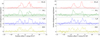 |
Fig. 8 Same as Fig. 7 but for IRAS 15082–4808. |
| In the text | |
|
Fig. 9 Normalised AARPs of molecular line brightness distributions for IRAS 15194–5115 (left), IRAS 15082–4808 (middle), and IRAS 07454–7112 (right). The vertical grey gridlines apply to the lower x axis in cm units. |
| In the text | |
|
Fig. 10 Examples of Gaussian fits to the AARPs: HCN (centrally peaked species, top panel) and CN (shell species, bottom panel), both towards IRAS 07454–7112. The solid blue lines show the mean AARPs and the dashed red lines show the Gaussian fits. The dash-dotted black Gaussians were obtained by deconvolving the beam from the Gaussian fit. The yellow lines show the HWHM distance from the centre of the beam-deconvolved Gaussian on either side of the peak, and the horizontal pink linse depicts the HWHM (for centrally peaked emission, top panel) or the FWHM (for shell emission, bottom panel) of the beam-deconvolved Gaussian. |
| In the text | |
|
Fig. 11 Estimates of the extents of the molecular line-emitting regions. The horizontal lines show the radial extent of the emitting regions, as determined through Gaussian fits, for each molecule towards IRAS 07454–7112 (yellow), IRAS 15082-4808 (red), and IRAS 15194–5115 (blue). The ♦ signs denote the positions of the emission peaks. The + signs indicate species for which the emissions from several isotopo-logues (see Sect. 4.3.2) were averaged to produce the AARP. The values of the emission extents and their uncertainties are listed in Table 5. |
| In the text | |
|
Fig. 12 Rotation temperatures (Trot, left panel) and total column densities (Ntot, right panel) obtained from population diagrams. The dashed vertical black line separates the shell species and the centrally peaked species. |
| In the text | |
|
Fig. 13 Molecular fractional abundances for the three stars (this work) and IRC +10216 (from the literature, see Table 7). The absolute abundances are shown in the top panel. The middle panel shows the abundances normalised to IRC +10216, and the bottom panel shows the abundances normalised to each star’s own C34S abundance. Uncertainties of these estimates are discussed in Sect. 4.5. |
| In the text | |
|
Fig. A.1 ALMA Band 3 line survey of IRAS 07454–7112 (black), IRAS 15082–4808 (blue; vertical offset of 0.1 Jy), and IRAS 15194–5115 (red; vertical offset of 0.2 Jy). Labels show the carrier molecule of the indicated emission. Red labels indicate tentative or unidentified detections, and green labels indicate lines that have been identified only in central-pixel spectra (not shown). The spectra from the combined data have been inserted in the respective frequency ranges (see Table 2). |
| In the text | |
|
Fig. C.1 C13CCCH, N=9-8, J=19/2-17/2 (85.201906 GHz) |
| In the text | |
|
Fig. C.2 C13CH, N=1-0, J=3/2-1/2 (85.232792 GHz) |
| In the text | |
|
Fig. C.3 c-C3H2, 21,2–10,1 (85.338894 GHz) |
| In the text | |
|
Fig. C.4 CC13CCH, N=9-8, J=17/2-15/2 (85.37033 GHz) |
| In the text | |
|
Fig. C.5 C4H, N=9-8, J=19/2-17/2 (85.634004 GHz) |
| In the text | |
|
Fig. C.6 C4H, N=9-8, J=17/2-15/2 (85.672582 GHz) |
| In the text | |
|
Fig. C.7 29SiO, 2-1 (85.759194 GHz) |
| In the text | |
|
Fig. C.8 H13CN, 1-0 (86.339921 GHz) |
| In the text | |
|
Fig. C.9 Si13CC, 41,4 – 31,3 (86.562636 GHz) |
| In the text | |
|
Fig. C.10 SiO, 2-1 (86.846985 GHz) |
| In the text | |
|
Fig. C.11 HN13C, 1-0 (87.090825 GHz) |
| In the text | |
|
Fig. C.12 C2H, N=1-0, J=3/2-1/2, F=1-1 (87.284105 GHz) |
| In the text | |
|
Fig. C.13 C2H, N=1-0, J=3/2-1/2, F=2-1 (87.316898 GHz) |
| In the text | |
|
Fig. C.14 C2H, N=1-0, J=1/2-1/2, F=1-0 (87.44647 GHz) |
| In the text | |
|
Fig. C.15 30SiS, 5-4 (87.550558 GHz) |
| In the text | |
|
Fig. C.16 H13CC13CN, 10-9 (87.773712 GHz) |
| In the text | |
|
Fig. C.17 H13C13CCN, 10-9 (87.841102 GHz) |
| In the text | |
|
Fig. C.18 HC5N, 33-32 (87.86363 GHz) |
| In the text | |
|
Fig. C.19 H13CCCN, 10-9 (88.166832 GHz) |
| In the text | |
|
Fig. C.20 Si34S, 5-4 (88.285828 GHz) |
| In the text | |
|
Fig. C.21 HCN, 1-0 (88.631602 GHz) |
| In the text | |
|
Fig. C.22 CC13CN, N=9-8, J=19/2-17/2 (88.7117 GHz) |
| In the text | |
|
Fig. C.23 CC13CN, N=9-8, J=17/2-15/2 (88.7302 GHz) |
| In the text | |
|
Fig. C.24 C3N, 9-8 (A) (89.0456 GHz) |
| In the text | |
|
Fig. C.25 C3N, 9-8 (B) (89.0643 GHz) |
| In the text | |
|
Fig. C.26 29SiS, 5-4 (89.103749 GHz) |
| In the text | |
|
Fig. C.27 I-C4H2, 103,8-93,7 (89.289791 GHz) |
| In the text | |
|
Fig. C.28 C6H, J=65/2-63/2 (90.093295 GHz) |
| In the text | |
|
Fig. C.29 HC13C13CN, 10-9 (90.204324 GHz) |
| In the text | |
|
Fig. C.30 HC5N, 34-33 (90.52589 GHz) |
| In the text | |
|
Fig. C.31 30SiC2, 40,4-30,3 (90.562283 GHz) |
| In the text | |
|
Fig. C.32 HC13CCN, 10-9 (90.593059 GHz) |
| In the text | |
|
Fig. C.33 HCC13CN, 10-9 (90.601777 GHz) |
| In the text | |
|
Fig. C.34 HNC, 1-0 (90.663568 GHz) |
| In the text | |
|
Fig. C.35 SiS, 5-4 (90.771564 GHz) |
| In the text | |
|
Fig. C.36 Si13CC, 40,4-30,3 (90.848527 GHz) |
| In the text | |
|
Fig. C.37 C8H, J=155/2-153/2 (90.92464 GHz) |
| In the text | |
|
Fig. C.38 HC3N, 10-9 (90.979023 GHz) |
| In the text | |
|
Fig. C.39 13CCCCH, N=10-9, J=21/2-19/2 (91.875516 GHz) |
| In the text | |
|
Fig. C.40 13CCCCH, N=10-9, J=19/2-17/2 (91.906057 GHz) |
| In the text | |
|
Fig. C.41 Si13CC, 42,3-32,2 (92.064397 GHz) |
| In the text | |
|
Fig. C.42 CCC13CH, N=10-9, J=21/2-19/2 (92.277495 GHz) |
| In the text | |
|
Fig. C.43 CCC13CH, N=10-9, J=19/2-17/2 (92.31491 GHz) |
| In the text | |
|
Fig. C.44 13CS, 2-1 (92.494308 GHz) |
| In the text | |
|
Fig. C.45 SiC2, 40,4-30,3 (93.063639 GHz) |
| In the text | |
|
Fig. C.46 HC5N, 35-34 (93.188123 GHz) |
| In the text | |
|
Fig. C.47 SiC2, 42,3-32,2 (94.245393 GHz) |
| In the text | |
|
Fig. C.48 C13CCCH, N=10-9, J=21/2-19/2 (94.670583 GHz) |
| In the text | |
|
Fig. C.49 C13CCCH, N=10-9, J=19/2-17/2 (94.708235 GHz) |
| In the text | |
|
Fig. C.50 CC13CCH, N=10-9, J=21/2-19/2 (94.814724 GHz) |
| In the text | |
|
Fig. C.51 CC13CCH, N=10-9, J=19/2-17/2 (94.853126 GHz) |
| In the text | |
|
Fig. C.52 C4H, N=10-9, J=21/2-19/2 (95.150389 GHz) |
| In the text | |
|
Fig. C.53 C4H, N=10-9, J=19/2-17/2 (95.188949 GHz) |
| In the text | |
|
Fig. C.54 SiC2, 42,2-32,1 (95.579381 GHz) |
| In the text | |
|
Fig. C.55 HC5N, 36-35 (95.850335 GHz) |
| In the text | |
|
Fig. C.56 C34S, 2-1 (96.41295 GHz) |
| In the text | |
|
Fig. C.57 H13CCCN, 11-10 (96.983001 GHz) |
| In the text | |
|
Fig. C.58 C33S, 2-1 (97.172064 GHz) |
| In the text | |
|
Fig. C.59 Si13CC, 41,3-31,2 (97.295257 GHz) |
| In the text | |
|
Fig. C.60 CS, 2-1 (97.980953 GHz) |
| In the text | |
|
Fig. C.61 C3H, J=9/2-7/2 (98.01207 GHz) |
| In the text | |
|
Fig. C.62 HC5N, 37-36 (98.512524 GHz) |
| In the text | |
|
Fig. C.63 CC13CN, N=10-9, J=21/2-19/2 (98.569 GHz) |
| In the text | |
|
Fig. C.64 C3N, 10-9 (A) (98.94 GHz) |
| In the text | |
|
Fig. C.65 C3N, 10-9 (B) (98.9588 GHz) |
| In the text | |
|
Fig. C.66 HC13C13CN, 11-10 (99.224259 GHz) |
| In the text | |
|
Fig. C.67 HC13CCN, 11-10 (99.651849 GHz) |
| In the text | |
|
Fig. C.68 HCC13CN, 11-10 (99.661467 GHz) |
| In the text | |
|
Fig. C.69 HC3N, 11-10 (100.076392 GHz) |
| In the text | |
|
Fig. C.70 13CCCCH, N=11-10, J=23/2-21/2 (101.06306 GHz) |
| In the text | |
|
Fig. C.71 13CCCCH, N=11-10, J=21/2-19/2 (101.09403 GHz) |
| In the text | |
|
Fig. C.72 HC5N, 38-37 (101.174677 GHz) |
| In the text | |
|
Fig. C.73 CCC13CH, N=11-10, J=23/2-21/2 (101.506343 GHz) |
| In the text | |
|
Fig. C.74 CCC13CH, N=11-10, J=21/2-19/2 (101.543766 GHz) |
| In the text | |
|
Fig. C.75 HC5N, 39-38 (103.836817 GHz) |
| In the text | |
|
Fig. C.76 C13CCCH, N=11-10, J=23/2-21/2 (104.13854 GHz) |
| In the text | |
|
Fig. C.77 C13CCCH, N=11-10, J=21/2-19/2 (104.17622 GHz) |
| In the text | |
|
Fig. C.78 CC13CCH, N=11-10, J=23/2-21/2 (104.29734 GHz) |
| In the text | |
|
Fig. C.79 CC13CCH, N=11-10, J=21/2-19/2 (104.33572 GHz) |
| In the text | |
|
Fig. C.80 C4H, N=11-10, J=23/2-21/2 (104.666566 GHz) |
| In the text | |
|
Fig. C.81 C4H, N=11-10, J=21/2-19/2 (104.70511 GHz) |
| In the text | |
|
Fig. C.82 30SiS, 6-5 (105.059203 GHz) |
| In the text | |
|
Fig. C.83 H13CCCN, 12-11 (105.799113 GHz) |
| In the text | |
|
Fig. C.84 Si34S, 6-5 (105.941503 GHz) |
| In the text | |
|
Fig. C.85 CCS, 89-78 (106.347726 GHz) |
| In the text | |
|
Fig. C.86 HC5N, 40-39 (106.49891 GHz) |
| In the text | |
|
Fig. C.87 29SiS, 6-5 (106.92298 GHz) |
| In the text | |
|
Fig. C.88 Si13CC, 51,5-41,4 (107.971477 GHz) |
| In the text | |
|
Fig. C.89 HC13CCN, 12-11 (108.710532 GHz) |
| In the text | |
|
Fig. C.90 HCC13CN, 12-11 (108.720999 GHz) |
| In the text | |
|
Fig. C.91 13CN, N=1-0, J=3/2-1/2 (108.782374 GHz) |
| In the text | |
|
Fig. C.92 C3N, 11-10 (A) (108.83425 GHz) |
| In the text | |
|
Fig. C.93 C3N, 11-10 (B) (108.853 GHz) |
| In the text | |
|
Fig. C.94 SiS, 6-5 (108.924301 GHz) |
| In the text | |
|
Fig. C.95 HC3N, 12-11 (109.173634 GHz) |
| In the text | |
|
Fig. C.96 CCC13CH, N=12-11, J=25/2-23/2 (110.735027 GHz) |
| In the text | |
|
Fig. C.97 CCC13CH, N=12-11, J=23/2-21/2 (110.772434 GHz) |
| In the text | |
|
Fig. C.98 HC5N, 42-41 (111.823024 GHz) |
| In the text | |
|
Fig. C.99 Si13CC, 50,5-40,4 (112.593212 GHz) |
| In the text | |
|
Fig. C.100 CN, N=1-0, J=1/2-1/2, F=1/2-3/2 (113.144157 GHz) |
| In the text | |
|
Fig. C.101 CN, N=1-0, J=1/2-1/2, F=3/2-1/2 (113.170492 GHz) |
| In the text | |
|
Fig. C.102 CN, N=1-0, J=1/2-1/2, F=3/2-3/2 (113.191279 GHz) |
| In the text | |
|
Fig. C.103 C13CCCH, N=12-11, J=23/2-21/2 (113.6442 GHz) |
| In the text | |
|
Fig. C.104 CC13CCH, N=12-11, J=23/2-21/2 (113.81808 GHz) |
| In the text | |
|
Fig. C.105 C4H, N=12-11, J=25/2-23/2 (114.182514 GHz) |
| In the text | |
|
Fig. C.106 C4H, N=12-11, J=23/2-21/2 (114.221042 GHz) |
| In the text | |
|
Fig. C.107 SiC2, 50,5-40,4 (115.382389 GHz) |
| In the text | |
|
Fig. C.108 Spectra of unidentified lines towards IRAS 15194-5115. The width of the region shaded in pink is twice the expansion velocity of the source CSE. The feature to the left of the 87.59 GHz line is a blend of the 30SiS 5−4 and SiN 2−1 lines. The u-lines are too weak to show any structure in the emission maps. They are not detected in the other two sources. |
| In the text | |
|
Fig. C.109 C4H, N=17-16 (161.796566 GHz) |
| In the text | |
|
Fig. C.110 SiS, 9-8 (163.376785 GHz) |
| In the text | |
|
Fig. C.111 HC3N, J=18-17 (163.753389 GHz) |
| In the text | |
|
Fig. C.112 SiC2, 7( 2, 6)- 6( 2, 5) (164.069091 GHz) |
| In the text | |
|
Fig. C.113 C3N N=17-16 (168.2043 GHz). |
| In the text | |
|
Fig. C.114 C4H, N=18-17 (171.310707 GHz) |
| In the text | |
|
Fig. C.115 29SiO, 4-3 (171.512796 GHz) |
| In the text | |
|
Fig. C.116 H13CN, J=2-1 (172.677851 GHz) |
| In the text | |
|
Fig. C.117 HC3N, J=19-18 (172.8493 GHz) |
| In the text | |
|
Fig. C.118 SiO, 4-3 (173.688238 GHz) |
| In the text | |
|
Fig. C.119 C2H, N=2-1 (174.663199 GHz) |
| In the text | |
|
Fig. C.120 HCN, J=2-1 (177.261111 GHz) |
| In the text | |
|
Fig. C.121 C4H, N=19-18 (180.824472 GHz) |
| In the text | |
|
Fig. C.122 HNC, J=2-1 (181.324758 GHz) |
| In the text | |
|
Fig. C.123 SiS, 10-9 (181.525218 GHz) |
| In the text | |
|
Fig. C.124 13CS, J=4-3 (184.981772 GHz) |
| In the text | |
|
Fig. C.125 SiC2, 8( 6, 3)- 7( 6, 2) (188.3857 GHz) |
| In the text | |
|
Fig. C.126 C4H N=20-19 (190.337804 GHz) |
| In the text | |
|
Fig. C.127 HC3N, J=21-20 (191.040299 GHz) |
| In the text | |
|
Fig. C.128 C34S, 4-3 (192.818457 GHz) |
| In the text | |
|
Fig. C.129 CS, 4-3 (195.954211 GHz) |
| In the text | |
|
Fig. C.130 SiS, 11-10 (199.672229 GHz) |
| In the text | |
|
Fig. C.131 C4H N=21-20 (199.850787 GHz) |
| In the text | |
|
Fig. C.132 HC3N, J=23-22 (209.230234 GHz) |
| In the text | |
|
Fig. C.133 C4H, N=22-21 (209.363302 GHz) |
| In the text | |
|
Fig. C.134 SiC2, 9( 2, 8)- 8( 2, 7) (209.892001 GHz) |
| In the text | |
|
Fig. C.135 SiC2, 9( 6, 4)- 8( 6, 3) (212.031878 GHz) |
| In the text | |
|
Fig. C.136 SiC2, 9( 4, 6)- 8( 4, 5) (213.208032 GHz) |
| In the text | |
|
Fig. C.137 SiC2, 9( 4, 5)- 8( 4, 4) (213.292337 GHz) |
| In the text | |
|
Fig. C.138 29SiS, 12-11 (213.81614 GHz) |
| In the text | |
|
Fig. C.139 29SiO, 5-4 (214.385752 GHz) |
| In the text | |
|
Fig. C.140 SiO, 5-4 (217.104919 GHz) |
| In the text | |
|
Fig. C.141 SiS, 12-11 (217.817663 GHz) |
| In the text | |
|
Fig. C.142 HC3N, J=24-23 (218.324723 GHz) |
| In the text | |
|
Fig. C.143 C4H N=23-22 (218.875369 GHz) |
| In the text | |
|
Fig. C.144 SiC2, 10( 0,10)- 9( 0, 9) (220.773685 GHz) |
| In the text | |
|
Fig. C.145 SiC2, 9( 2, 7)- 8( 2, 6) (222.009386 GHz) |
| In the text | |
|
Fig. C.146 HC3N J=25-24 (227.418905 GHz) |
| In the text | |
|
Fig. C.147 C3N, N=23-22 (227.5539 GHz) |
| In the text | |
|
Fig. C.148 C4H, N=24-23 (228.386962 GHz) |
| In the text | |
|
Fig. C.149 Si34S, 13-12 (229.500868 GHz) |
| In the text | |
|
Fig. C.150 13CS, J=5-4 (231.220685 GHz) |
| In the text | |
|
Fig. C.151 29SiS, 13-12 (231.626673 GHz) |
| In the text | |
|
Fig. C.152 SiC2, 10( 2, 9)- 9( 2, 8) (232.53407 GHz) |
| In the text | |
|
Fig. C.153 SiC2, 10( 6, 5)- 9( 6, 4) (235.712998 GHz) |
| In the text | |
|
Fig. C.154 SiS, 13-12 (235.961363 GHz) |
| In the text | |
|
Fig. C.155 HC3N, J=26-27 (236.512789 GHz) |
| In the text | |
|
Fig. C.156 SiC2, 10( 4, 7)- 9( 4, 6) (237.150018 GHz) |
| In the text | |
|
Fig. C.157 SiC2, 10( 4, 6)- 9( 4, 5) (237.331309 GHz) |
| In the text | |
|
Fig. C.158 C3N, N=24-23 (237.44415 GHz) |
| In the text | |
|
Fig. C.159 C4H, N=25-24 (237.89806 GHz) |
| In the text | |
|
Fig. C.160 C34S, 5-4 (241.016089 GHz) |
| In the text | |
|
Fig. C.161 SiC2, 11( 0,11)-10( 0,10) (241.367708 GHz) |
| In the text | |
|
Fig. C.162 C33S, 5-4 (242.91361 GHz) |
| In the text | |
|
Fig. C.163 CS, 5-4 (244.935556 GHz) |
| In the text | |
|
Fig. C.164 Si34S, 14-13 (247.146242 GHz) |
| In the text | |
|
Fig. C.165 C3N, N=25-24 (247.334 GHz) |
| In the text | |
|
Fig. C.166 C4H, N=26-25 (247.408643 GHz) |
| In the text | |
|
Fig. C.167 SiC2, 10( 2, 8)- 9( 2, 7) (247.52912 GHz) |
| In the text | |
|
Fig. C.168 29SiS, 14-13 (249.435412 GHz) |
| In the text | |
|
Fig. C.169 SiS, 14-13 (254.103211 GHz) |
| In the text | |
|
Fig. C.170 30SiO, 6-5 (254.216656 GHz) |
| In the text | |
|
Fig. C.171 C4H, N=27-26 (256.918691 GHz) |
| In the text | |
|
Fig. C.172 29SiO, 6-5 (257.255213 GHz) |
| In the text | |
|
Fig. C.173 H13CN, J=3-2 (259.011798 GHz) |
| In the text | |
|
Fig. C.174 SiC2, 11( 6, 6)-10( 6, 5) (259.433309 GHz) |
| In the text | |
|
Fig. C.175 SiO, 6-5 (260.518009 GHz) |
| In the text | |
|
Fig. C.176 SiC2, 11( 4, 8)-10( 4, 7) (261.150695 GHz) |
| In the text | |
|
Fig. C.177 SiC2, 11( 4, 7)-10( 4, 6) (261.509329 GHz) |
| In the text | |
|
Fig. C.178 C2H, N=3-2 (262.064986 GHz) |
| In the text | |
|
Fig. C.179 30SiS, 15-14 (262.585033 GHz) |
| In the text | |
|
Fig. C.180 Si34S, 15-14 (264.789719 GHz) |
| In the text | |
|
Fig. C.181 HCN, J=3-2 (265.886434 GHz) |
| In the text | |
|
Fig. C.182 C4H, N=28-27 (266.428184 GHz) |
| In the text | |
|
Fig. C.183 C3N, N=27-26 (267.11225 GHz) |
| In the text | |
|
Fig. C.184 29SiS, 15-14 (267.242218 GHz) |
| In the text | |
|
Fig. C.185 Lines from the APEX Band 7 (272–376 GHz) survey of IRAS 15194-5115, which have been used in this work. The grey shaded regions represent the channels used for calculating the integrated intensities of the lines, reported in Table B.2. The dotted vertical line marks the systemic velocity of the source. |
| In the text | |
|
Fig. D.1 AARPs (solid) and Gaussian fits (dashed) for SiO (left) and SiS (right) emission. |
| In the text | |
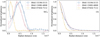 |
Fig. D.2 Same as Fig. D.1 but for SiC2 (left) and CS (right) emission. |
| In the text | |
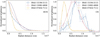 |
Fig. D.3 Same as Fig. D.1 but for HCN (left) and CN (right) emission. |
| In the text | |
|
Fig. D.4 Same as Fig. D.1 but for C2H (top left), C3H (top right), C4H (bottom left), and c-C3H2 (bottom right) emission |
| In the text | |
|
Fig. D.5 Same as Fig. D.1 but for HC3N (top left), C3N (top right), HC5N (bottom left), and HNC (bottom right) emission |
| In the text | |
|
Fig. E.1 Population diagrams for SiO for the three stars, IRAS 15194–5115 (left), IRAS 15082–4808 (centre), and IRAS 07454–7112 (right). The solid line (red) is the best-fit linear model to the data (black). Rotation temperatures, Trot, and source-averaged column densities, Ntot, are listed in the legends. Circle and square points denote lines observed with ALMA and APEX, respectively. Hollow circles denote lines for which data combination (see Sect. 3.3) was performed. |
| In the text | |
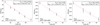 |
Fig. E.2 Same as Fig. E.1 but for 29SiO. |
| In the text | |
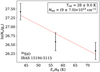 |
Fig. E.3 Same as Fig. E.1 but for 30SiO. |
| In the text | |
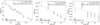 |
Fig. E.4 Same as Fig. E.1 but for SiS. |
| In the text | |
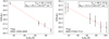 |
Fig. E.5 Same as Fig. E.1 but for 29SiS. |
| In the text | |
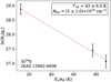 |
Fig. E.6 Same as Fig. E.1 but for Si34S. |
| In the text | |
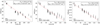 |
Fig. E.7 Same as Fig. E.1 but for SiC2. |
| In the text | |
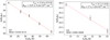 |
Fig. E.8 Same as Fig. E.1 but for CS. |
| In the text | |
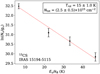 |
Fig. E.9 Same as Fig. E.1 but for 13CS. |
| In the text | |
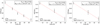 |
Fig. E.10 Same as Fig. E.1 but for C34S. |
| In the text | |
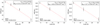 |
Fig. E.11 Same as Fig. E.1 but for HCN. |
| In the text | |
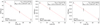 |
Fig. E.12 Same as Fig. E.1 but for H13CN. |
| In the text | |
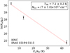 |
Fig. E.13 Same as Fig. E.1 but for HNC. |
| In the text | |
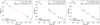 |
Fig. E.14 Same as Fig. E.1 but for HC3N. |
| In the text | |
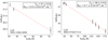 |
Fig. E.15 Same as Fig. E.1 but for C3N. |
| In the text | |
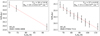 |
Fig. E.16 Same as Fig. E.1 but for HC5N. |
| In the text | |
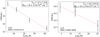 |
Fig. E.17 Same as Fig. E.1 but for C2H. |
| In the text | |
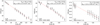 |
Fig. E.18 Same as Fig. E.1 but for C4H. |
| In the text | |
Current usage metrics show cumulative count of Article Views (full-text article views including HTML views, PDF and ePub downloads, according to the available data) and Abstracts Views on Vision4Press platform.
Data correspond to usage on the plateform after 2015. The current usage metrics is available 48-96 hours after online publication and is updated daily on week days.
Initial download of the metrics may take a while.