| Issue |
A&A
Volume 642, October 2020
The XXL Survey: third series
|
|
|---|---|---|
| Article Number | A124 | |
| Number of page(s) | 25 | |
| Section | Cosmology (including clusters of galaxies) | |
| DOI | https://doi.org/10.1051/0004-6361/202038982 | |
| Published online | 13 October 2020 | |
The XXL Survey
XLII. Detection and characterisation of the galaxy population of distant galaxy clusters in the XXL-N/VIDEO field: A tale of variety⋆
1
Department of Physics & Astronomy, University of Victoria, 3800 Finnerty Road, Victoria, British Columbia V8W 2Y2, Canada
e-mail: This email address is being protected from spambots. You need JavaScript enabled to view it.
2
AIM, CEA, CNRS, Université Paris-Saclay, Université Paris Diderot, Sorbonne Paris Cité 91191 Gif-sur-Yvette, France
3
INAF – IASF Milan, Via A. Corti 12, 20133 Milano, Italy
4
INAF – Osservatorio di Astrofisica e Scienza dello Spazio di Bologna, Via Piero Gobetti 93/3, 40129 Bologna, Italy
5
INFN, Sezione di Bologna, Viale Berti Pichat 6/2, 40127 Bologna, Italy
6
Academia Sinica Institute of Astronomy and Astrophysics (ASIAA), No. 1, Section 4, Roosevelt Road, Taipei 10617, Taiwan
7
Université Aix-Marseille, CNRS, LAM (Laboratoire d’Astrophysique de Marseille) UMR 7326, 13388 Marseille, France
8
Sub-department of Astrophysics, University of Oxford, Denys Wilkinson Building, Keble Road, Oxford OX1 2DL, UK
9
European Southern Observatory, Alonso de Cordova 3107, Vitacura, Santiago 19001, Chile
10
Department of Physics & Astronomy, University of the Western Cape, Private Bag X17, Bellville, Cape Town 7535, South Africa
11
Institute for Astronomy & Astrophysics, Space Applications & Remote Sensing, National Observatory of Athens, 15236 Palaia Penteli, Greece
12
CEA Saclay, DRF/Irfu/DEDIP/LILAS, 91191 Gif-sur-Yvette Cedex, France
13
Argelander Institut für Astronomie, Universität Bonn, Auf dem Huegel 71, 53121 Bonn, Germany
14
INAF-Astronomical Observatory of Padova, Vicolo dell’Osservatorio 5, 35122 Padova, Italy
Received:
20
July
2020
Accepted:
3
September
2020
Abstract
Context. Distant galaxy clusters provide an effective laboratory in which to study galaxy evolution in dense environments and at early cosmic times.
Aims. We aim to identify distant galaxy clusters as extended X-ray sources that are coincident with overdensities of characteristically bright galaxies.
Methods. We used optical and near-infrared data from the Hyper Suprime-Cam and VISTA Deep Extragalactic Observations (VIDEO) surveys to identify distant galaxy clusters as overdensities of bright, zphot ≥ 0.8 galaxies associated with extended X-ray sources detected in the ultimate XMM extragalactic survey (XXL).
Results. We identify a sample of 35 candidate clusters at 0.80 ≤ z ≤ 1.93 from an approximately 4.5 deg2 sky area. This sample includes 15 newly discovered candidate clusters, ten previously detected but unconfirmed clusters, and ten spectroscopically confirmed clusters. Although these clusters host galaxy populations that display a wide variety of quenching levels, they exhibit well-defined relations between quenching, cluster-centric distance, and galaxy luminosity. The brightest cluster galaxies (BCGs) within our sample display colours that are consistent with a bimodal population composed of an old and red sub-sample together with a bluer, more diverse sub-sample.
Conclusions The relation between galaxy masses and quenching seem to already be in place at z ∼ 1, although there is no significant variation in the quenching fraction with the cluster-centric radius. The BCG bimodality might be explained by the presence of a younger stellar component in some BCGs, but additional data are needed to confirm this scenario.
Key words: galaxies: clusters: general / galaxies: distances and redshifts / galaxies: evolution / galaxies: high-redshift / galaxies: photometry / X-rays: galaxies: clusters
Based on observations obtained with XMM-Newton, an ESA science mission with instruments and contributions directly funded by ESA Member States and NASA.
© ESO 2020
1. Introduction
Galaxy clusters are the most massive gravitationally bound structures at any epoch. Clusters are dark matter dominated (∼85% of the total mass), while a hot X-ray emitting intracluster medium (ICM) accounts for most of the baryonic mass of the cluster (Plionis et al. 2008). Stars and galaxies correspond to less than 5% of the total mass (Plionis et al. 2008). Clusters provide one of the most extreme environments in the Universe: Infalling galaxies are stripped of their gas by the intracluster medium ram pressure (e.g. Poggianti et al. 2004, 2008, 2016, 2019; Jaffé et al. 2018; Tonnesen 2019), while the centre is one of the densest environments found in space.
The formation and evolution of the most massive giant elliptical galaxies, the brightest cluster galaxies (BCGs), is intimately related to the cluster environment. The BCGs are located near the gravitational centre of their host galaxy clusters and they exhibit unique properties, such as distinct luminosity and surface brightness profiles, and/or supersolar metallicities (e.g. Oemler 1976; Tremaine & Richstone 1977; Dressler 1978; Von Der Linden et al. 2007; Loubser et al. 2009). The classical formation scenario of these galaxies, proposed by De Lucia & Blaizot (2007), is one of early star formation (mostly before z ∼ 3), which is quickly suppressed by active galactic nuclei (AGN) feedback (e.g Croton et al. 2006), and of progressive, late assembly via gas-poor mergers.
At low redshifts, BCG properties are generally consistent with this picture (e.g. Stott et al. 2008, 2011; Lidman et al. 2012; Bellstedt et al. 2016; Edwards et al. 2020); although, several examples of low to moderately star-forming BCGs have been reported in individual, X-ray bright clusters (e.g. Egami et al. 2006; Bildfell et al. 2008; Stott et al. 2008; Pipino et al. 2009; Loubser et al. 2009, 2016; Rawle et al. 2012; Green et al. 2016). However, there is gathering evidence against the classical scenario at z ≳ 1: Webb et al. (2015) and McDonald et al. (2016) report evidence of significant in-situ star formation in ∼20% and ∼90% of their z > 1 samples, respectively. The triggering mechanism of this star formation remains unknown; although, McDonald et al. (2016) have suggested galaxy interactions, which is a possibility that is supported by recent simulations (Rennehan et al. 2020).
The cessation of star formation activity, referred to as quenching, plays an important role in the evolution of galaxies – both for the BCG and within the cluster environment as a whole. Indeed, galaxies appear to evolve at an accelerated rate in clusters as opposed to in the field at all redshifts (e.g. Alberts et al. 2014; Nantais et al. 2017; Foltz et al. 2018; Jian et al. 2018; Pintos-Castro et al. 2019; Strazzullo et al. 2019), although it is unclear at which redshift the passive fraction in clusters becomes greater than in the field (e.g. Strazzullo et al. 2013, 2019; Brodwin et al. 2013; Alberts et al. 2014; Nantais et al. 2017). Quenching also depends on galaxy mass in the sense that higher mass galaxies are more quenched than those of a lower mass (e.g. Muzzin et al. 2012; Balogh et al. 2016; Kawinwanichakij et al. 2017; Jian et al. 2018; Pintos-Castro et al. 2019). Since the most massive galaxies typically reside in the cluster core, mass and environmental effects are difficult to disentangle (e.g. Balogh & McGee 2010; Muzzin et al. 2012; Kawinwanichakij et al. 2017; Jian et al. 2018; Pintos-Castro et al. 2019) and they require large samples of well-characterised galaxy clusters.
Galaxy clusters may be identified by employing a range of techniques. Optical and infrared (IR) imaging surveys identify clusters as overdensities of galaxies (e.g. Postman et al. 1996; Gladders & Yee 2000, 2005; Euclid Collaboration 2019). The red-sequence algorithm (Gladders & Yee 2000, 2005), as was used in the recent Spitzer Adaptation of the Red-sequence Survey (SpARCS; e.g. Wilson et al. 2006, 2009), identifies overdensities exhibiting colours that are consistent with the red-sequence at a given redshift. However, this red-sequence selection may introduce a bias towards clusters with enhanced red galaxy populations (e.g. Donahue et al. 2002; Willis et al. 2018). An alternative approach is to identify clusters using the properties of the intra-cluster medium, either indirectly via the Suyaev-Zel’dovich effect (e.g. Zel’dovich & Sunyaev 1969; Sunyaev & Zel’dovich 1970, 1972, 1980a,b; Carlstrom et al. 2002; Bleem et al. 2015) or directly via X-ray bremsstrahlung emission (e.g. Gursky et al. 1972; Sarazin 1986; Pierre et al. 2004, 2016, hereafter XXL Paper I; Willis et al. 2018). X-ray selection has been successfully used in the past to find clusters of galaxies, either alone (e.g. Vikhlinin et al. 1998; Clerc et al. 2012) or with the aid of optical data (e.g. Gioia et al. 1990; Böhringer et al. 2001; Willis et al. 2013). There is tentative evidence that such clusters sometimes display smaller red-sequence galaxy populations than optically selected clusters (Donahue et al. 2002; Willis et al. 2018), but a drawback is that X-ray selected samples can exhibit a bias towards relaxed, cool-core clusters (e.g. Eckert et al. 2011; Rossetti et al. 2017; Willis et al. 2018) and lower BCG-X-ray peak distances (e.g. Lavoie et al. 2016, hereafter XXL Paper XV; Rossetti et al. 2016), hence the need for cluster studies with various, complementary selected samples (e.g. Donahue et al. 2002; Sadibekova et al. 2014; Bleem et al. 2015; Willis et al. 2018).
In this paper we employ a multi-wavelength data set constructed as part of the XMM-XXL survey to identify distant galaxy clusters and study their galaxy populations. The XMM-XXL survey covers 50 deg2 divided into two equal fields: XXL-North and XXL-South (XXL-N and XXL-S; (XXL Paper I)). Each field is constructed from a mosaic of 10 ks XMM pointings. The present paper focuses on a contiguous sub-area of the XXL-N field covering 5.3 deg2, XMM-SERVS, which has been observed with an exposure time of 46 ks per pointing (Chen et al. 2018). This deeper sub-area of XMM data is accompanied by a range of multi-wavelength optical and IR data (see XXL Paper I), including a high-quality data set generated by the Visible and Infrared Survey Telescope for Astronomy (VISTA) Deep Extragalatic Observations (VIDEO) survey (Jarvis et al. 2013). We refer to the 4.5 deg2 field with overlapping deep XMM and VIDEO data as the XXL-N/VIDEO field (see Fig. 1).
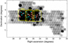 |
Fig. 1. VIDEO footprints overlaid on XXL-N exposure map. VIDEO covers eight VISTA footprints, the following three of them are within the XXL-N field: XMM1, XMM2, and XMM3. The darker part of the exposure map corresponds to the 46 ks exposure of the XMM-SERVS field. The cyan and salmon crosses correspond to the respective locations of the confirmed clusters and candidate clusters in our sample. |
This paper presents the identification and characterisation of a sample of distant galaxy clusters selected from the XXL-N/VIDEO field. In Sects. 2 and 3, we describe the identification and composition of the cluster sample. In Sect. 4, we compute the fraction of quenched galaxies within the cluster sample and as a function of salient properties, such as the cluster-centric distance and galaxy luminosity. In Sect. 5 we identify a sample of BCGs from the cluster sample and investigate the properties of their stellar populations and their star formation histories. In Sect. 6 we discuss the possible causes of the variety of observed cluster quenching fractions and of the BCG colour bimodality before summarising our main conclusions in Sect. 7. We employ a WMAP9 cosmology characterised by H0 = 69.32 km s−1 Mpc−1, Ωm = 0.2865, and ΩΛ = 0.7135 (Hinshaw et al. 2013). At redshifts of 1 and 1.5, an angular scale of 1 arcmin corresponds to 489 and 518 kpc, respectively. All photometry is quoted in the AB magnitude system.
The present paper relies on the new version of the XXL-XMM pipeline (V4), which is still in development, and on the related X-ray parameters and images. Compared to the V3 pipeline dealing with individual XMM observations on which all previous XXL publications were based, the V4 pipeline processes co-added observations that are assembled into 1 × 1 deg2 mosaics. By dealing with pointing overlaps, V4 ensures reaching the ultimate sensitivity at any position (Faccioli et al. 2018, hereafter XXL Paper XXIV). This is especially important for the VIDEO region, which is characterised by a high level of redundancies.
Throughout this paper, we consider that a cluster is confirmed if at least three galaxies within the X-ray emission have matching spectroscopic redshifts or if an obvious BCG has a spectroscopic redshift (Adami et al. 2018, hereafter XXL Paper XX). The expression “unconfirmed clusters” is used to refer to candidate clusters with insufficient information in order to be spectroscopically confirmed. Cluster names with the prefix “XLSSC” pertain to spectroscopically confirmed clusters only and they may be found in XXL Paper XX. The prefix “3XLSS” refers to X-ray sources that are a part of the Chiappetti et al. (2018, XXL Paper XXVII) catalogue. New V4 detections are labelled by the prefix “XLSSU”.
2. Observations and cluster detection
In this paper, we attempt to identify significant galaxy overdensities observed in optical-IR imaging data associated with extended X-ray sources. We employed the galaxy photometric redshift (from the VIDEO catalogue) distribution of positive matches to select candidate distant clusters at zphot ≥ 0.8.
2.1. X-ray data
In short, the XAMIN pipeline tests four models to characterise the detected sources, which generate likelihood estimates for point, extended, and double point sources, as well as an extended plus point source. This latter model, denoted AC, is intended to flag extended sources that are significantly contaminated by a central AGN. The coordinates of the X-ray source presented in Sect. 3 are based on the centre of the best-fit model. Cluster sources are further classified into C1 and C2 on the basis of pipeline parameters extent and extent_likelihood. The C1 sample corresponds to an almost pure sample of bright clusters, while the C2 sample, which is fainter, allows for up to 50% of the sample to be misclassified point sources (see Pacaud et al. 2006, XXL Paper XXIV). False C2 are routinely excluded by the examination of X-ray and optical overlays for cluster candidates below z = 1.
It is important to mention that the choice of the numerical pipeline parameter values used to define the C1 and C2 criteria are still those that are based on the detections performed with the V3 pipeline from simulated individual XMM observations. These criteria will be revised when the final V4 is fully validated and applied to mosaic simulations. However, we do not expect drastic changes in the class parameters since they are based on likelihoods. This situation does not impact the current study because it does not explicitly involve the cluster selection function at any stage.
2.2. Optical and near infrared photometry
The VIDEO observations consist of IR imaging undertaken with the VISTA telescope in the YJHKs photometric bands. In the XMM-SERVS field, these observations reach 5σ depths of at least 25.1, 24.7, 24.2, and 23.8 mag within 2 arcsec circular apertures for YJHKs, respectively (Adams et al. 2020). The VIDEO catalogue also contains additional imaging data consisting of the Canada-France-Hawaii Telescope Legacy Survey Deep-1 field (CFHTLS-D1) and of the deep “layer” of the Hyper Suprime-Camera (HSC) Subaru Strategic Program (HSC-SSP, Aihara et al. 2018a,b). The ultra-deep “layer” of HSC-SSP overlaps with the XMM1 field.
The photometric redshift analysis included in the catalogue employs an i-band selected source list where photometry in additional bands is obtained by applying SExtractor to astrometrically-matched pixel data at other wavelengths. In addition, we employed HSC-SSP iz and VIDEO JKs photometry from this catalogue to study the properties of candidate cluster member galaxies directly. The HSC-SSP deep data have 5σ limiting magnitudes of 25.4 and 24.6 in the i and z bands, respectively, and the ultra-deep data have limiting magnitudes of 26.4 and 26.3 (Adams et al. 2020).
Photometric redshifts for sources in the VIDEO catalogue are computed using the LEPHARE photometric redshift code (Ilbert et al. 2006). The code employs the COSMO template set (Ilbert et al. 2009), including 32 templates from Polletta et al. (2007) and from Bruzual & Charlot (2003). Dust attenuation follows a Calzetti et al. (2000) law, and the intergalactic medium absorption treatment is based on Madau (1995). Further details are provided by Adams et al. (2020).
2.3. Identification of galaxy clusters
We performed four steps to select candidate clusters from our X-ray sample and followed a similar procedure to that of Willis et al. (2013). Each step is summarised below:
-
Convolve the photometric redshift histogram for bright galaxies with a matched Gaussian filter chosen to match the properties of redshift peaks of spectroscopically confirmed clusters. Galaxies are selected to be brighter than the characteristic luminosity, L*, along the line-of-sight of each X-ray source (i.e. a 1 arcmin radius aperture centred on the X-ray best-fit model centre).
-
Identify overdensities corresponding to a bright galaxy excess of ≳4 and display the position of potential members on colour images together with X-ray emission contours.
-
Examine the i − z and z − J colour-magnitude diagrams of each candidate cluster.
-
Employ a Gaussian model of the photometric redshift distribution of selected overdensities to estimate a refined mean cluster redshift and its standard deviation.
Figure 2 presents a visual summary of these four steps. Similar images of the other candidate clusters are presented in Appendix B.
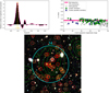 |
Fig. 2. Visual summary of the cluster identification process. Top left: background subtracted and Gaussian filtered photometric redshift distribution of the bright galaxies within the central arcmin of candidate 14. The dashed line indicates the highest bin in the redshift spike. Top right: i − z CMD plot of the galaxies above the VIDEO 5σ limit within 1 arcmin of the centre. The green squares indicate the galaxies with photometric redshifts that are consistent with the mean redshift plus or minus 1.5 times the standard deviation of the most accurate Gaussian modelling of the redshift spike. The blue lozenges indicate galaxies with redshifts that are consistent with the sidewings of the most accurate Gaussian model, up to three times the standard deviation. The deep pink line indicates where the red sequence should be at this redshift, based on the best fit calculated in Sect. 4.1. The light pink region indicates the uncertainty on this red-sequence model, which is also calculated in Sect. 4.1. Bottom panel: example of a Megacam r and i filter as well as a VIDEO H filter image for candidate 14, which is one of our candidate clusters. The cyan circle delimits the region within 1 arcmin of the X-ray best fit model centre, which is marked by a yellow cross. The red and brown circles highlight the bright galaxies with a redshift corresponding to the cluster photometric peak redshift ±0.02 and to the cluster redshift ±0.06, respectively. Darker circles indicate the galaxies outside the central region. The BCG is circled in white. The X-ray contours in green are logarithmically distributed in ten levels between the maximum and minimum emission observed in a 7 × 7 arcmin2 box around the X-ray source. |
The first step of the identification process is to select galaxies and AGN that might be associated with each X-ray source. We selected the galaxies and AGN sources by employing their goodness-of-fit when compared to stellar, galactic, and AGN templates (see Jarvis et al. 2013). Because galaxies in clusters are more likely to host radio-loud AGN than field galaxies (Best et al. 2007), we kept AGN and discarded only the star-like objects. Then, we selected objects within 1 arcmin of the considered X-ray detection. We refer to these objects as the “field-of-view” galaxies.
We selected bright galaxies in the field-of-view by employing luminosity function arguments: We computed the apparent magnitude of M*, assuming M* = −22.26 in the Ks band using Cirasuolo et al. (2010) with no evolution from z ∼ 3 to z ∼ 0 and a k-correction described by the bandwidth term. Galaxies brighter than the expected apparent m* magnitude at their photometric redshift were retained. We applied a further photometric cut based on the 5σ depth of the VIDEO Ks band, discarding any galaxy fainter than 23.8. The latter cut is important beyond z ∼ 1.4, where m* is fainter than the VIDEO 5σ limit.
Selected field-of-view galaxies were then binned in photometric redshift space, over the interval 0.2 < zphot < 3.2. Galaxies were sampled in bins of 0.04 in photometric redshift since this is the redshift iteration step employed in the photometric redshift analysis. We then used the catalogue distribution to perform a background subtraction by applying the same selection steps described above and by scaling the number distribution by the relative size of our field-of-view compared to that of the full the catalogue, that is to say
 (1)
(1)
where NFOV is the number of galaxies in a particular redshift bin in our field-of-view, Ncat is the number of galaxies listed in the catalogue in the corresponding redshift bin after applying the same cuts, rFOV is the 1 arcmin radius we used to select galaxies associated with an X-ray detection, and Acat is the catalogue area.
To identify structures in the photometric redshift histogram along the line-of-sight to each extended X-ray source, we employed a matched Gaussian filter with a full width at half maximum (FWHM) that is equal to 0.12 in redshift (i.e. three bins). The properties of the Gaussian profile are based on the unfiltered redshift peaks associated with spectroscopically confirmed clusters.
2.4. Overdensity assessment
We performed a visual inspection of all C1, C2, and AC X-ray sources that display a signal that is consistent with > 4 galaxies at a single photometric redshift. We typically employed riH images from CFHTLS and VIDEO with the candidate members indicated in addition to X-ray emission contours (see Fig. 2). We further generated i − z and z − J colour magnitude diagrams of each candidate cluster in order to determine if a red sequence is present.
The overdensity finding method provides a first estimate for the candidate cluster redshift based on the median redshift of the highest bins (see Fig. 2, bottom left panel). To refine this estimate, we modelled each candidate redshift signal as a Gaussian and employed the 13 central bins of the non-filtered redshift signal. We then used the Gaussian mean as the cluster redshift and the standard deviations as an estimate of the uncertainty.
3. The cluster sample
3.1. Sample selection
We processed a total of 284 extended X-ray detections within the XXL-N/VIDEO region. This parent sample generated a sample of 35 candidate distant galaxy clusters. Table 1 and Fig. 3 present these clusters, each of which represents a detection with a significance of approximately four galaxies or more in a photometric redshift bin satisfying zphot ≥ 0.8 (see also Fig. 1). Of these 35 candidate clusters, ten have been spectroscopically confirmed while 15 are presented here for the first time. Ten additional candidates have been previously identified as distant clusters; however, to our knowledge, they have never been spectroscopically confirmed (see Olsen et al. 2007; Finoguenov et al. 2010; Durret et al. 2011; Wen & Han 2011; Licitra et al. 2016, XXL Paper XX).
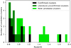 |
Fig. 3. Histogram of the candidate cluster redshifts. The black bars correspond to the spectroscopic redshifts of the confirmed clusters and the green bars represent the photometric redshifts of the candidate clusters, which were either previously observed (dark green) or newly detected (lighter green). |
Detections above z ∼ 0.8.
Nine of the confirmed cluster detections were confirmed by prior spectroscopy (e.g. Pierre et al. 2006; Willis et al. 2013, XXL Paper XX), including one at z = 1.803 (Andreon et al. 2014). With the spectroscopic redshifts listed in the CESAM database1 (XXL Paper XX), we were able to confirm one additional cluster (candidate 3), bringing the total number of confirmed clusters to ten. All of these X-ray detections meet our criteria for candidate clusters.
Four confirmed distant clusters in this area (Pierre et al. 2006; Papovich et al. 2010, XXL Paper XX) are not a part of our sample because their coordinates do not correspond to a V4 C1, C2, or AC detection. This is the case for a z = 1.62 cluster (Papovich et al. 2010). Although IRC-0218A and our detections at similar redshifts possess comparable masses (IRC-0218A M200 is 7.7 ± 3.9 × 10¹³ M⊙), IRC-0218A X-ray emission is completely dominated by a point source (Pierre et al. 2012).
We nevertheless applied our optical and IR detection criteria to those four clusters. Two clusters satisfied these criteria, including IRC-0218A, and were included in our photometric redshift accuracy assessment (see the following section). The clusters XLSS J022609.9-043120 and XLSSC 203 (see Pierre et al. 2006, XXL Paper XX) located at z = 0.82 and z = 1.077, respectively, did not satisfy them. Since V4 works on co-added and thus deeper images, we expect its source characterisation to be more reliable.
3.2. Photometric redshift accuracy
To estimate the reliability of our photometric redshift estimates for the candidate clusters, we compared the spectroscopic redshift of 12 confirmed clusters in the field (six clusters listed in (XXL Paper XX), four from Pierre et al. 2006; Papovich et al. 2010; Willis et al. 2013; Andreon et al. 2014, and two other confirmed clusters in the XXL-N/VIDEO area) to the photometric redshift generated by the cluster finding procedure. Figure 4 shows the result of this comparison. At z ∼ 1, the differences between the photometric and spectroscopic redshifts fall well within the photometric redshift error estimates. These error bars represent the standard deviation of the best-fitting Gaussian model. For the two high redshift clusters, the photometric redshifts seem to underestimate the spectroscopic values. Therefore, we calculated the root mean square (RMS) of the z ∼ 1 and z ≳ 1.5 clusters separately. We obtained 0.02 and 0.14, respectively. For now on, we use these RMS values as the uncertainties on the photometric redshifts.
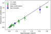 |
Fig. 4. Comparison between the spectroscopic redshifts of confirmed clusters within the XXL-N/VIDEO overlap and the corresponding photometric overdensities in the VIDEO catalogue. The error bars correspond to the standard deviation of the Gaussian model that fits the photometric spike best. All clusters, except two (not included), were detected in optical. The green dots are the clusters that are a part of our sample, while the blue squares are not included in our sample since they do not meet our X-ray selection criteria. The magenta diamond is the newly confirmed candidate 3. The dashed line represents the ideal case, where zphot = zspec. |
3.3. Clusters’ estimated masses
Following a similar methodology as the second data release of XXL, we used scaling relations to provide an estimate of the mean parameters for clusters for which the data quality is not sufficient enough to perform a direct spectral fit. A detailed description is provided in Sect. 4.3 of XXL Paper XX, and we provide a brief overview here. We estimated count-rates in the pn data in the [0.5–2] keV band within 300 kpc of the cluster centre, using the Bayesian approach to the fixed aperture photometry measurement outlined in Willis et al. (2018). We then converted this count-rate to the corresponding X-ray luminosity by adopting an initial gas temperature, a metallicity fixed to 0.3 times the solar value (as tabulated in Anders & Grevesse 1989), and the cluster spectroscopic (when available) or photometric redshift. With the same initial guess as to the temperature, we estimated r500, scal from the mass-temperature relation constrained from a subset of 105 XXL clusters that have both measured HSC lensing masses and X-ray temperatures (see Umetsu et al. 2020). We stress that here we use a M500 | TX relation, which was obtained using the Bayesian regression scheme implemented in the LIRA package (Sereno 2016; Sereno et al. 2016), and not the TX − M500 relation reported in Umetsu et al. (2020). The luminosity was then extrapolated from 300 kpc to r500, scal, assuming a β-model for the cluster emissivity with parameters (rc, β) = (0.15r500, scal, 2/3). Then a new temperature was evaluated using the best-fit result for the luminosity-temperature relation quoted in Table 6 of XXL Paper XX (XXL fit). The iteration on the gas temperature was stopped when the input and output values agreed within 5%, and in general the process converges after 2–3 steps. The uncertainties on the derived parameters, and in particular the masses, are obtained by the propagation of errors on the scaling parameters, including the measured correlation among them.
3.4. Other clusters in XXL-N/VIDEO
There are 54 previously confirmed clusters that are either within or overlap with the XXL-N/VIDEO field (XXL Paper XX). Of these, 47 are located at z < 0.8 with the remaining seven clusters located at z ≥ 0.8. These seven clusters correspond to a surface density of 1.6 distant clusters per square degree. This number represents a lower limit because some known clusters associated with an extended X-ray detection (e.g. JKCS 041, a z = 1.803 confirmed cluster Andreon et al. 2014) were excluded from XXL Paper XX compilation.
Adding all of our detections would bring this number up to approximately 8.2 clusters per square degree, with a flux limit of 1.7 × 10⁻¹⁵ erg cm−2 s−1 in the [0.5–2] keV band (Chen et al. 2018). This represents 3.6 times and 0.51 times the surface densities reached by Willis et al. (2013) and Finoguenov et al. (2010) with depths of 1 × 10⁻¹⁴ erg cm−2 s−1 and 2 × 10⁻¹⁵ erg cm−2 s−1 in the [0.5–2] keV band, respectively.
4. Quenching and star formation in clusters
The fraction of quenched galaxies in a sample of distant, X-ray selected galaxy clusters has the potential to provide an unbiased view of the star formation conditions in massive, virialised structures. In this section, we compute the fraction of quenched galaxies within the XXL-N/VIDEO distant cluster sample, focussing on the clusters at z < 1.4, because the catalogue 5σ magnitude limit restricts the number of selected galaxies beyond that redshift. We achieved this by employing four related analysis techniques, while intending to investigate whether each provides consistent results. Only the galaxies brighter than the 5σ limit in J and Ks are used in these computations.
-
The first employs the i − z colour histogram of background corrected galaxies in the field of each candidate cluster. This colour space distribution is then modelled using two Gaussian functions to represent the red sequence and the blue cloud (see Fig. 5).
-
The second method employs the same background corrected colour distribution as above, but it employs a single colour cut to divide the distribution into quenched and star-forming galaxies.
-
The third method selects cluster galaxies using photometric redshift and then applies the boundary method used in the method above (2).
-
The fourth method is similar to method 2 with the additional constraint that each galaxy, including the background, must be brighter than L* at the candidate cluster redshift. The L* evolutionary k-correction is computed using the results from method 1 (see Fig. 6).
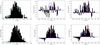 |
Fig. 5. Illustration of two steps of the first method. Left panels: i − z colour histograms in two fields-of-view (candidate 13 and candidate 8) where the default background (pink line) is either too high or too low. The adjusted background is overplotted in green. Middle panels: resulting colour distribution is the background is left unadjusted. For comparison purposes, the Gaussian models of the red sequence and the blue cloud are shown in pink and blue, respectively; although, they were computed with an adjusted background. The mauve dash-dotted line is the “boundary” used in method 2, 3, and 4. Right panels: colour distribution once the background was adjusted. |
4.1. First quenching method
The first step consists of defining the appropriate area within which one can select field-of-view galaxies for each cluster. Some previous studies (e.g. Wetzel et al. 2012; Pintos-Castro et al. 2019) analyse the quenched and star-forming fraction up to several virial radii. However, since several of our fields appear to contain secondary overdensities, we chose to restrict our analysis to closer to the cluster centre, namely within a radius of 1.35 Mpc around the X-ray coordinates. A radius of 1.35 Mpc corresponds to approximately 1.5 times the value of r500 for a 1 × 10¹⁴ M⊙ galaxy cluster (Chen et al. 2007) and to an angle of 2.76 arcminutes at z = 1. We further selected galaxies with a photometric redshift between 0.60 and 2.04, both in the cluster field and background catalogue, and sampled the resulting distributions into 0.04 wide bins in i − z colour.
We then corrected this field-of-view distribution using the same method as applied in Eq. (1). A visual inspection reveals that the resulting colour distribution is bimodal (see Fig. 5). We modelled this bimodal colour distribution using two Gaussian functions - one representing the red sequence and the other the blue cloud. In some fields, we note that the background correction is either too large or too small to yield to a clear bimodal distribution, resulting in poor fits or even in a non-convergent fitting algorithm (candidate 7). In such cases, we adjusted the background correction by up to 20% before determining whether the adjusted background results in an improved fit. Figure 5 presents the effect of an unadjusted background on the colour distribution on two typical fields. Although both cases that are too high and too low are presented, the former concerns only four clusters. One of these clusters is confirmed (candidate 3) and two others (including the case presented in Fig. 5) are among the sample of other photometric studies (see Olsen et al. 2007; Wen & Han 2011; Licitra et al. 2016). Thus, most of them are unlikely to be false detections.
Three out of the eight clusters with an increased background lie in overlaps between two VIDEO footprints and thus have, according to Jarvis et al. (2013) longer exposure times. Moreover, two additional clusters are in the XMM1 field, which is a part of the ultra-deep layer of the HSC-SPP survey, and they thus possess 1 to 1.5 mag deeper photometry in the i and z band (see Adams et al. 2020).
The quenched fraction was then computed as the integral of the best-fitting red sequence Gaussian profile, divided by the sum of the integrals of the blue cloud and red sequence Gaussian profiles. Some clusters were removed from the analysis. We removed 1, 4, 10, 21, and 24 since there are indications of more than one overdensity along the line-of-sight to each of these X-ray sources. Candidate clusters at z ≥ 1.4 were also removed, resulting in a sample of 21 candidate clusters.
Next, we investigate whether the Gaussian modelling produces consistent average star formation histories, that is whether the red sequence colour can be adequately described by a simple stellar population model. We used Flexible Stellar Population Models (FSPS; see Conroy et al. 2009; Conroy & Gunn 2010; Foreman-Macke et al. 2014), modelling the red sequence stellar population with an exponentially decreasing star formation rate characterised by an e-folding timescale τ, displaying solar metallicity and no dust. We generated a grid of models with two free parameters: We tested 100 formation redshifts between 4 and 16, and 100 τ values between 0.1 and 2.5 Gyr for a total of 10 000 models. The model providing the best fit has a formation redshift of 16 with a characteristic time of 1.19 Gyr and a reduced  , corresponding to a rejection probability of 24%. The red sequence displayed on the colour-magnitude diagram (CMD) plot in Fig. 2 is based on this model. The associated uncertainty is the standard deviation of the difference of red sequence colours, as predicted by the model, and the Gaussian modelling results. We also used this fit to compute the evolutionary and K-correction associated with the characteristic luminosity used in method 4.
4.2. Other quenching methods
The second method to identify quenched galaxies employs the same colour binning and background subtraction procedure as the one used by the Gaussian method described above. We specified the colour where the blue and red Gaussian models are equal as the boundary between the red sequence and the blue cloud. We further restricted the colour interval by rejecting any galaxy that is redder than 2.5 times the standard deviation of the red Gaussian or bluer than 2.5 times the standard deviation of the blue Gaussian. We performed a fractional calculation within the affected bins where those boundaries fall within a colour bin.
The third method does not include the area-corrected background subtraction used in the first two methods, but it instead selects cluster members based on their photometric redshift. Any galaxy within the field-of-view and with a redshift consistent with the cluster mean redshift plus or minus 1.5 times its standard deviation (calculated in Sect. 2.4) is considered as a cluster member. We then selected the red sequence and blue cloud members using the colour boundaries defined in method 2.
All the methods described above employ the 5σ limit of the VIDEO catalogue in J and Ks bands as a magnitude selection threshold. The fourth quenching method is essentially the same as method 2, yet with an evolving magnitude limit based on the values of L* in J and Ks bands computed using our best-fitting FSPS model for the red sequence, that is, including both an evolutionary and k-correction (see Fig. 6). As in Sect. 2.3, we assume a characteristic absolute magnitude of −22.26 at z = 0 (see also Cirasuolo et al. 2010).
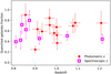 |
Fig. 6. Fraction of quenched galaxies as a function of the redshift, according to method 4, for each VIDEO candidate, excluding candidates 1, 4, 10, 21, and 24 and the candidate clusters above z = 1.4. Spectroscopically confirmed clusters are indicated by squares, and circles are used to show the other ones. The error bars are the propagation on the Poissonian uncertainties on the integrals of the red sequence and the blue cloud models. |
A comparison between method 1 and the other methods is presented in Fig. 7. Each method generates similar quenched fractions compared to method 1. Within the limited variation of the approaches taken by each method, this indicates that the quenched fractions are robust from method to method. The few clusters for which the quenched fractions obtained by method 1 are more than 1.5 times the standard deviation above or below the mean are identified and highlighted. From now on, we focus on the results from method 4.
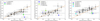 |
Fig. 7. Comparison between the quenched fractions obtained by methods 1 and 2 (left panel), methods 1 and 3 (middle panel), or methods 1 and 4 (right panel). The error bars are based on the Poissonian uncertainties on the number of quenched galaxies in the cluster and on the number of galaxies in the considered field-of-view. The background uncertainty included is estimated to 5% of the unscaled background subtraction since we adjusted the subtracted background by steps of 10%. Clusters that have quenching ratios above or below 1.5 times the standard deviation of |

4.3. Quenching results
Figure 6 shows the quenched fraction results of the fourth method and indicates that there are a wide variety of quenching levels within the interval 0.8 ≤ z ≤ 1.2. The wide range of computed quenched fractions is nominally consistent with the expectation expressed in Sect. 1 that the X-ray selection of galaxy clusters should be less biased to the properties of their member galaxies than optical and IR overdensity methods.
Next, we test, despite the range of quenched fractions, whether there is a consistent variation in the quenched fraction as a function of cluster-centric distance within the sample of clusters as a whole. We computed the quenched fraction for each cluster within three equal radial annuli out to 1.35 Mpc. We then computed the mean cluster quenched fractions as a function of the radius into two groups based upon the total quenched fraction, that is, we stacked those clusters that are quenched at the level greater than the median quenched fraction into one group and those quenched at less than the median level into another.
We then investigated if the quenched fraction depends on the galaxy luminosity. We computed the quenched fraction in three bins of J/Ks luminosities (0.5 to 1 L*, 1 to 2 L*, and 2 to 4 L*). Once again, the results for each cluster were stacked on the basis of their overall quenching level. This test is limited to z < 1.4, because beyond this, 0.5 L* falls below the 5σ magnitude cut.
Figure 8 displays no significant trend between the mean quenched fraction and the cluster-centric radius, especially for the highly quenched half of the sample. We note, however, a slight increase in the quenched fraction towards the centre of the lowly quenched cluster, suggesting a weak dependence of the quenched fraction with the distance. The bottom panels of Fig. 8 show that more luminous galaxies are more quenched, although the variation is less pronounced in highly quenched clusters.
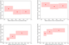 |
Fig. 8. Top row: mean quenched fraction for each distance bin, for the low quenching (left) and high quenching (right) candidate clusters. Symbols mark the mean quenched fraction, while the shaded regions represent the bin size (x axis) and the standard deviation (y axis) of the quenched fraction. Bottom row: mean quenched fraction for each luminosity bin according to method 2/4 (method 2 is equivalent to method 4 in this context). Luminosities are expressed in terms of L*. We stress that L*, the absolute magnitude, changes with the redshift to reflect the passive evolution of a quenched galaxy. In the interval 0.8 ≤ z < 1.4, the absolute magnitude M* varies from −22.87 to −23.14 in the Ks band and the corresponding stellar masses from 1.45 × 10¹¹ M⊙ to 1.47 × 10¹¹ M⊙. Again, clusters are divided into low quenching (left) and a high quenching (right) groups. These plots only include clusters below z = 1.4 in order to mitigate the selection effects of the catalogue 5σ limit. |
5. Brightest cluster galaxies
To identify candidate BCGs within each galaxy cluster, we initially noted that 80% of BCGs are located within 0.1 virial radii of the cluster’s X-ray emission peak (Lin & Mohr 2004). They are usually, but interestingly not always (e.g. Lange et al. 2018), the most luminous galaxy in the cluster. We, therefore, selected galaxies within 225 kpc of the X-ray detection coordinates where this distance corresponds to approximately 15% of the virial radius of a 1 × 10¹⁴ M⊙ cluster (we added an extra 5% to account for possible offsets between the X-ray best-fit model centres and the X-ray emission peaks). We then applied a luminosity cut to select galaxies brighter than 3 L* in J and Ks bands (using the model computed in Sect. 4.1 to compute evolutionary effects and a full k-correction). If the luminosity cut resulted in less than three candidate BCGs, we extended the cut to 2.5 L*. If there still remained less than three galaxies, we enlarged our search radius to 450 kpc. We implemented this three candidate limit because we noticed that some fields contained faint stars that were misclassified as galaxies or quasars in the VIDEO catalogue.
To identify spurious candidates, we subsequently performed a visual check of the BCG candidates, while paying special attention to the brightest and second brightest candidates. We also flagged, but did not remove, candidates with unreliable photometry, such as candidates within the halo of a star or blended sources. We then created i − z, z − J, and J − Ks colour magnitude diagrams of the central 225 kpc of each cluster to determine which candidate BCGs possess colours that are consistent with the cluster redshift. This step also resulted in the benefit that it identified galaxies with magnitudes and colours comparable to the two most luminous candidates that might have been missed by the previous cuts. We then selected up to three potential BCGs within each cluster. In most of the clusters considered, a single BCG candidate is prominent. In cases with more than one candidate BCG, we used the Ks band luminosities to select the most likely BCG, followed by the projected cluster-centric distance if Ks band magnitudes were similar. When possible, we used the CESAM spectroscopic database to check the redshift of our selected BCG candidates and made adjustments in the case of obvious inconsistencies with the estimated cluster redshift.
We compared our BCG list to Wen & Han (2011), XXL Paper XV, and Ricci et al. (2018, hereafter XXL Paper XXVIII), even though we have only 15, 1, and 5 clusters in common, respectively. Those three studies have slightly different BCG selection criteria: Wen & Han (2011) used the i, i*, or the r band depending on the data available, while XXL Paper XV and XXL Paper XXVIII used z and i′ band photometry as their main selection criterion, respectively. Each of them used larger search radii and, in the case of XXL Paper XXVIII, a stricter photometric redshift cut.
We found the same BCGs for 11 of the 15 shared candidates with Wen & Han (2011). When our selection disagrees, the BCG from Wen & Han (2011) is either fainter than our selected candidate (candidates 13 and 18), it possesses an incompatible spectroscopic redshift (candidate 12), or it is an obvious foreground galaxy (candidate 1). For candidate 20, which is the only candidate we have in common with XXL Paper XV, our BCG selection agrees. In the case of clusters that we have in common with XXL Paper XXVIII, four of the five common clusters have matching BCGs (candidates 3, 8, 20, and 21). For candidate 2, they selected our second-best BCG candidate, which, unlike our chosen candidate, possesses a spectroscopic redshift. However, the preferred candidate of XXL Paper XXVIII is fainter than our chosen candidate in the i, z, J, and Ks band.
As a final step, we employed FSPS to generate a suite of stellar population models, which we compared to the J − Ks colours of our total sample of BCGs as a function of redshift. We tested 100 different formation redshifts between three and 16, in combination with 100 different metallicities between 0.1 and 5 Z⊙. We assumed an instantaneous starburst, no dust extinction, and a Salpeter initial mass function (Salpeter 1955). We then tested the effect of including a third free parameter, using ten different formation redshifts and 50 metallicities within the same intervals as above. We first tested the effect of dust, which was calculated as a power law with a −0.7 index, with 25 dust obscuration percentages covering 0 to 99.3%. We also investigated the effect of permitting a dust-free, exponentially decreasing star formation rate (SFR) employing 25 τ values between 0.004 and 1 Gyr.
We limited the stellar population modelling to BCGs drawn from clusters in the interval 0.8 ≤ z < 1.4 and also removed BCGs with unreliable photometry. We also excluded candidate 10 because no suitable BCG candidate was identified. We thus performed our fits with a sample of 23 BCGs. The models described above generate fits that are characterised by reduced χ2 (hereafter noted  ), which is approximately equal to 3.5 in each case. The left panel of Fig. 9 presents these best fitting models and their associated confidence intervals. An examination of that figure indicates that the single model fits might well be averaging two groups of BCGs, namely a group with red J − Ks colours and a comparatively bluer group. We refer to these groupings as red and blue BCGs. Only one of the BCGs in the blue sample is bluer than the red sequence model, which is displayed as a magenta dotted line in Fig. 9. This discrepancy is discussed further in Sect. 6.2.
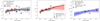 |
Fig. 9. Best fits for different sub-samples. In each case, three fits were tested: a simple model, in which the metallicity and the formation redshift, assuming an instantaneous starburst, were allowed to vary; and two other models where an additional parameter was allowed to vary, which is the dust content in one case (green dashed line) or the characteristic timescale of the star formation, assuming an exponentially decreasing star formation rate, instead of an instantaneous starburst (purple dash-dotted line). For comparative purposes, we also display the best fit model of Lidman et al. (2012) and our red sequence fit on two panels (the dotted cyan and dotted magenta lines, respectively; see Sect. 4.1). The shaded region corresponds to the 95% confidence region for the simplest model tested and the darker zone corresponds to the 68% confidence region. Left panel: best fits for all BCGs at 0.8 ≤ z ≤ 1.2, except candidate 10 and three BCGs with known photometric problems. Red galaxies are a part of the red sample and blue galaxies are a part of the blue sample. Middle panel: best fits for the red BCGs sub-sample. Right panel: best fits for the blue sub-sample. |
We find that none of the fitted stellar population models appear to capture the overall slope of colour versus redshift for the combined BCG sample. However, we noted with interest that the stellar population model of Lidman et al. (2012) appears to provide an effective method to segregate the red and blue BCGs. We therefore segregated the red and blue BCGs by employing the colour difference with respect to the Lidman et al. (2012) model colours as a function of redshift (see Fig. 10, left panel). Having split the BCGs into red and blue on the basis of this criterion, we then applied the FSPS fitting procedure described above to both populations and performed a final check of the BCG colour evolution versus redshift with respect to the best-fitting red and blue models (Fig. 10, centre and right panels). All three approaches generate the same division between red and blue BCGs.
 |
Fig. 10. Division of the blue and red BCGs based on their colour difference with a reference model; the dashed line represents the limit between the two groups. Left: division based on the Lidman et al. (2012) model. Middle: assessment of our sample bimodality based on the red BCGs best fit. Right: same as the left side, but based on the best fit of blue BCGs. |
Treating the red and blue BCGs as separate populations provides a significant improvement to the quality of the stellar population fits (see Fig. 9, middle and right panels). Tables 2 and 3 give the  and best parameter fits for every model tested. The uncertainties are based on the 1σ photometry errors. Despite relatively good
  (1.140 for the simplest model), none of the red BCG fits seem to be able to capture the slope of the J − Ks colours of the high-redshift half of the sample. Both the simple and dusty models perform similarly, but the plausibility of the latter seems questionable since it features a starlight dust absorption percentage of 61%.
Summary of the stellar population fits obtained for the red BCGs.
Summary of the stellar population fits obtained for the blue BCGs.
For the blue BCGs, there is no visible slope discrepancy between the data and the model. However, the  are larger than in the case of red BCGs, which is probably because none of the applied models include a term for intrinsic scatter. In fact, the 95% confidence interval of the simplest model, which also has the minimum
  , is barely spawning the variety of colours observed in the blue BCGs. This may indicate that the blue BCG population is too diverse to be represented by a single stellar population model.
Nevertheless, we computed the BCG stellar masses for the red and the blue BCGs, using the parameters from the simple model (i.e the instantaneous starburst model with no dust). We adopted a similar approach as in Lidman et al. (2012) by computing the mass as the quotient between the observed and the modelled flux density in the Ks band, correcting with the model stellar mass. To estimate the uncertainties, we computed the Ks band fluxes of every model enclosed in the 68% χ2 confidence region. We then considered their standard deviation as the uncertainty on the flux and propagated this error to the mass.
The results are presented in Tables 4 and 5. The mean masses are 5 ± 1 × 10¹¹ M⊙ and 2.8 ± 0.6 × 10¹¹ M⊙ for the red and blue BCGs, respectively.
Positions and stellar masses of the red BCGs.
Positions and stellar masses of the blue BCGs.
6. Discussion
6.1. Cluster quenched fractions
Figure 6 presents a wide variety of quenched fractions, with no clear trend; despite this, only the most luminous (massive) galaxies are visible at higher redshifts. The fourth method of computing the quenched fraction incorporates a luminosity cut specifically intended to mitigate this bias. However, although this method generates slightly higher quenched fractions (except for the two lowest redshift clusters in our sample; see Fig. 7), it does not otherwise affect the apparent diversity of quenched fractions. There is thus no evidence of evolution with redshift in Fig. 6.
The results presented in Sect. 4.3 demonstrate a link between the quenched fraction and the Ks band luminosity, although the link seems weaker for the highly quenched half of our sample. The Ks band luminosities are a proxy for galaxy stellar masses, assuming dust extinction is negligible. This type of link has been observed before (e.g. Peng et al. 2010, 2012; Muzzin et al. 2012; Balogh et al. 2016; Kawinwanichakij et al. 2017; Jian et al. 2018; Pintos-Castro et al. 2019); however, whether this is due to mass-dependent galaxy evolution and/or to the environment remains an open question.
We observe no significant evidence that the quenching fraction varies with the cluster-centric distance, although the quenched fraction is slightly higher towards the centre of the lowly quenched clusters in our sample – an observation that is in agreement with previous studies (e.g. Muzzin et al. 2012; Pintos-Castro et al. 2019). The more quenched half of our sample possesses levels of quenching above 70% in all bins, which might be because only galaxies above L* are included in this profile and since bright galaxies tend to be slightly more quenched at all radii.
6.2. Potential bimodal brightest cluster galaxy population
The J − Ks colours of the candidate BCGs in the distant cluster sample are not consistent with the properties of a single, passively-evolving stellar population. There is tentative evidence for a bimodal distribution of BCG colours. In separating the sample employing the fiducial stellar population model of Lidman et al. (2012), we find that the colours of the redder BCGs in our sample are consistent with an older, instantaneous burst of metal-rich stars, whereas the bluer BCG colours are more diverse and they are possibly related to a younger component in the stellar population.
Despite the variety of colours, only one of the BCGs is bluer than the red sequence model computed in Sect. 4.1 (see also Fig. 9). This might indicate that BCG stellar populations have different properties (such as metallicity) than the average quenched galaxies in cluster, as suggested by some low-redshift studies (e.g. Von Der Linden et al. 2007; Loubser et al. 2009).
Figure 11 shows the degeneracy between metallicity and formation redshift as applied to the stellar population models describing the two BCG samples. We observe that the 95% confidence regions of the two BCG samples do not overlap, supporting the idea that the stellar populations of the blue and red BCGs are indeed different. The confidence intervals for the blue sample are centred on lower metallicities than the red sample regions, while formation redshift also tends to be lower; although, the confidence regions of both models extend over a wide range of redshifts.
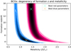 |
Fig. 11. Contour plots for the red and blue BCG sub-samples showing the |

Based on the stellar population analysis, one might infer that blue BCGs have formed more recently than the red ones. However, Li & Han (2007) reported that when more than one stellar population is present, the age and metallicity obtained by colours alone might be biased towards the younger and more metal-rich stars. Therefore, the blue BCGs might be bluer because they have experienced either an extended star formation episode or more than one bursts in the past. In these types of scenarios, differences in the duration of the star formation or in the relative importances and epochs of the secondary bursts would account for the spread in colour observed in the bluer BCGs.
One factor that may trigger a star formation episode is a cooling flow. Several studies have reported the existence of blue, moderately star-forming BCGs in cool-core clusters at low to moderate redshifts (e.g. Egami et al. 2006; Bildfell et al. 2008; Stott et al. 2008; Loubser et al. 2009, 2016; Pipino et al. 2009; Rawle et al. 2012; Green et al. 2016). Since X-ray selected clusters are biased towards relaxed clusters (Rossetti et al. 2017), this might partially explain why the blue BCGs represent a significant part of our sample.
Alternatively, statistical studies based on IR- (e.g. Webb et al. 2015, Bonaventura et al. 2017) or SZ-selected clusters (e.g. McDonald et al. 2016) have shown that in-situ star formation is an important mechanism at z ≳ 1, which is possibly triggered by galaxy interactions (McDonald et al. 2016). This suggests that a range of BCG colours might be a part of every high-redshift sample, regardless of the sample selection.
One limitation of the current analysis is that the fitted stellar population models are unable to accommodate the slope of the high-redshift end of the red sample J − Ks colour variation with redshift (see Fig. 9) and that no BCGs are red beyond z = 1.05. This suggests that the stars making up the red BCGs formed later or evolve faster than predicted by our model. The former is supported by the degeneracy between formation redshift and metallicity. The best-fitting formation redshift, zform ∼ 12, might be considered high compared to the predictions of the most recent simulations (e.g. Ragone-Figueroa et al. 2018; Rennehan et al. 2020); however, it is consistent with recent observations (Hashimoto et al. 2018; Willis et al. 2020).
Dust extinction might be evoked to explain why these objects are so red. Indeed, a fit including dust provides an equivalent statistical description of the red BCGs (see Table 2), although we note that the colour of a model stellar population is degenerate between the star formation history, metallicity, and dust obscuration. For this reason, we prefer a simple, dust free model for the analysis of the red BCG population.
Ultimately, the current data available for the BCGs sample are unable to provide a definitive explanation as to the blue and red dichotomy. The acquisition of rest-frame optical spectroscopy of several BCGs of both groups is needed in order to get a more accurate and thorough picture of the star formation history of these objects (e.g. Lonoce et al. 2015, 2020; Belli et al. 2017; Saracco et al. 2019).
7. Summary
We have identified a sample of 35 X-ray-selected distant galaxy clusters in the XXL-N/VIDEO field and performed a preliminary analysis of their galaxy populations. Clusters were selected as extended X-ray sources (C1, C2, or AC) coincident with overdensities of bright galaxies in photometric redshift space. Of the 35 candidate clusters at zphot ≥ 0.8, ten are spectroscopically confirmed clusters, and a further 15 are presented here for the first time. The ten remaining clusters have been detected previously but never confirmed.
The sample of clusters displays a wide variety of quenched fractions, a result that is nominally consistent with the assertion made in Sect. 1 that selecting clusters on the ICM properties is insensitive to the star formation history of their member galaxies. The relationship between the galaxy luminosity and quenched fraction appears to be in place at z ∼ 1, although we do not observe a significant variation in the quenched fraction with the cluster-centric radius.
The sample of BCGs is inconsistent with a single stellar population model. The observed distribution is bimodal in colour and is consistent with an old, passive population and a possibly younger, relatively bluer, and more diverse population. Although we are unable to provide a definite explanation for this split, we suggest that the blue BCGs may have experienced either an extended or more than one star-formation episode.
Acknowledgments
AT is supported by the Natural Sciences and Engineering Research Council of Canada (NSERC) Postgraduate Scholarship-Doctoral Program. JPW acknowledges support from the NSERC Discovery Grant program. The Saclay group acknowledges long-term support from the Centre National d’Etudes Spatiales (CNES). This work was supported by the Programme National Cosmology et Galaxies (PNCG) of CNRS/INSU with INP and IN2P3, co-funded by CEA and CNES. NA acknowledges funding from the Science and Technology Facilities Council (STFC) Grant Code ST/R505006/1. RAAB is supported by the Glasstone Foundation, MJJ and RAAB acknowledge support from the Oxford Hintze Centre for Astrophysical Surveys which is funded through generous support from the Hintze Family Charitable Foundation and the award of the STFC consolidated grant (ST/N000919/1). XXL is an international project based around an XMM Very Large Programme surveying two 25 deg2 extragalactic fields at a depth of ∼6 × 10⁻¹⁵ erg cm−2 s−1 in the [0.5–2] keV band for point-like sources. The XXL website is http://irfu.cea.fr/xxl. Multi-band information and spectroscopic follow-up of the X-ray sources are obtained through a number of survey programmes, summarised at http://xxlmultiwave.pbworks.com/. This work is based on data products from observations made with ESO Telescopes at the La Silla Paranal Observatory under ESO programme ID 179.A- 2006 and on data products produced by the Cambridge Astronomy Survey Unit on behalf of the VIDEO consortium. This research has made use of the NASA/IPAC Extragalactic Database (NED), which is funded by the National Aeronautics and Space Administration and operated by the California Institute of Technology.
References
- Adami, C., Giles, P., Koulouridis, E., et al. 2018, A&A, 620, A5 (XXL Paper XX) [NASA ADS] [CrossRef] [EDP Sciences] [Google Scholar]
- Adams, N. J., Bowler, R. A. A., Jarvis, M. J., et al. 2020, MNRAS, 494, 1771 [CrossRef] [Google Scholar]
- Aihara, H., Arimoto, N., Armstrong, R., et al. 2018a, PASJ, 70, S4 [NASA ADS] [Google Scholar]
- Aihara, H., Armstrong, R., Bickerton, S., et al. 2018b, PASJ, 70, S8 [NASA ADS] [Google Scholar]
- Alberts, S., Pope, A., Brodwin, M., et al. 2014, MNRAS, 437, 437 [NASA ADS] [CrossRef] [Google Scholar]
- Anders, E., & Grevesse, N. 1989, Geochim. Cosmochim. Acta, 53, 197 [Google Scholar]
- Andreon, S., Newman, A. B., Trinchieri, G., et al. 2014, A&A, 565, A120 [NASA ADS] [CrossRef] [EDP Sciences] [Google Scholar]
- Balogh, M. L., & McGee, S. L. 2010, MNRAS, 402, L59 [NASA ADS] [CrossRef] [Google Scholar]
- Balogh, M. L., McGee, S. L., Mok, A., et al. 2016, MNRAS, 456, 4364 [NASA ADS] [CrossRef] [Google Scholar]
- Belli, S., Genzel, R., Förster Schreiber, N. M., et al. 2017, ApJ, 841, L6 [NASA ADS] [CrossRef] [Google Scholar]
- Bellstedt, S., Lidman, C., Muzzin, A., et al. 2016, MNRAS, 460, 2862 [NASA ADS] [CrossRef] [Google Scholar]
- Best, P. N., von der Linden, A., Kauffmann, G., Heckman, T. M., & Kaiser, C. R. 2007, MNRAS, 379, 894 [NASA ADS] [CrossRef] [Google Scholar]
- Böhringer, H., Schuecker, P., Guzzo, L., et al. 2001, A&A, 369, 826 [NASA ADS] [CrossRef] [EDP Sciences] [Google Scholar]
- Bildfell, C., Hoekstra, H., Babul, A., & Mahdavi, A. 2008, MNRAS, 389, 1637 [NASA ADS] [CrossRef] [Google Scholar]
- Bleem, L. E., Stalder, B., de Haan, T., et al. 2015, ApJS, 216, 27 [NASA ADS] [CrossRef] [Google Scholar]
- Bonaventura, N. R., Webb, T. M. A., Muzzin, A., et al. 2017, MNRAS, 469, 1259 [NASA ADS] [CrossRef] [Google Scholar]
- Brodwin, M., Stanford, S. A., Gonzalez, A. H., et al. 2013, ApJ, 779, 138 [NASA ADS] [CrossRef] [Google Scholar]
- Bruzual, G., & Charlot, S. 2003, MNRAS, 344, 1000 [NASA ADS] [CrossRef] [Google Scholar]
- Calzetti, D., Armus, L., Bohlin, R. C., et al. 2000, ApJ, 533, 682 [NASA ADS] [CrossRef] [Google Scholar]
- Carlstrom, J. E., Holder, G. P., & Reese, E. D. 2002, ARA&A, 40, 643 [NASA ADS] [CrossRef] [Google Scholar]
- Chen, C.-T. J., Brandt, W. N., Luo, B., et al. 2018, MNRAS, 478, 2132 [NASA ADS] [CrossRef] [Google Scholar]
- Chen, Y., Reiprich, T. H., Böhringer, H., Ikebe, Y., & Zhang, Y.-Y. 2007, A&A, 466, 805 [NASA ADS] [CrossRef] [EDP Sciences] [Google Scholar]
- Chiappetti, L., Fotopoulou, S., Lidman, C., et al. 2018, A&A, 620, A12 (XXL Paper XXVII) [NASA ADS] [CrossRef] [EDP Sciences] [Google Scholar]
- Cirasuolo, M., McLure, R. J., Dunlop, J. S., et al. 2010, MNRAS, 401, 1166 [NASA ADS] [CrossRef] [Google Scholar]
- Clerc, N., Sadibekova, T., Pierre, M., et al. 2012, MNRAS, 423, 3561 [NASA ADS] [CrossRef] [Google Scholar]
- Conroy, C., & Gunn, J. E. 2010, ApJ, 712, 833 [NASA ADS] [CrossRef] [Google Scholar]
- Conroy, C., Gunn, J. E., & White, M. 2009, ApJ, 699, 486 [NASA ADS] [CrossRef] [Google Scholar]
- Croton, D. J., Springel, V., White, S. D. M., et al. 2006, MNRAS, 365, 11 [NASA ADS] [CrossRef] [Google Scholar]
- De Lucia, G., & Blaizot, J. 2007, MNRAS, 375, 2 [NASA ADS] [CrossRef] [Google Scholar]
- Donahue, M., Scharf, C. A., Mack, J., et al. 2002, ApJ, 569, 689 [NASA ADS] [CrossRef] [Google Scholar]
- Dressler, A. 1978, ApJ, 223, 765 [NASA ADS] [CrossRef] [Google Scholar]
- Durret, F., Adami, C., Cappi, A., et al. 2011, A&A, 535, A65 [NASA ADS] [CrossRef] [EDP Sciences] [Google Scholar]
- Eckert, D., Molendi, S., & Paltani, S. 2011, A&A, 526, A79 [NASA ADS] [CrossRef] [EDP Sciences] [Google Scholar]
- Edwards, L. O. V., Salinas, M., Stanley, S., et al. 2020, MNRAS, 491, 2617 [CrossRef] [Google Scholar]
- Egami, E., Misselt, K. A., Rieke, G. H., et al. 2006, ApJ, 647, 922 [NASA ADS] [CrossRef] [Google Scholar]
- Euclid Collaboration (Adam, R., et al.) 2019, A&A, 627, A23 [CrossRef] [EDP Sciences] [Google Scholar]
- Faccioli, L., Pacaud, F., Sauvageot, J.-L., et al. 2018, A&A, 620, A9 (XXL Paper XXIV) [NASA ADS] [CrossRef] [EDP Sciences] [Google Scholar]
- Finoguenov, A., Watson, M. G., Tanaka, M., et al. 2010, MNRAS, 403, 2063 [NASA ADS] [CrossRef] [Google Scholar]
- Foltz, R., Wilson, G., Muzzin, A., et al. 2018, ApJ, 866, 136 [NASA ADS] [CrossRef] [Google Scholar]
- Foreman-Macke, D., Sick, J., & Johnson, B. 2014, Python-fsps: Python bindings to FSPS (v0.1.1) [Google Scholar]
- Gioia, I. M., Maccacaro, T., Schild, R. E., et al. 1990, ApJS, 72, 567 [NASA ADS] [CrossRef] [Google Scholar]
- Gladders, M. D., & Yee, H. K. C. 2000, ApJ, 120, 2148 [Google Scholar]
- Gladders, M. D., & Yee, H. K. C. 2005, ApJS, 157, 1 [NASA ADS] [CrossRef] [Google Scholar]
- Green, T. S., Edge, A. C., Stott, J. P., et al. 2016, MNRAS, 461, 560 [CrossRef] [Google Scholar]
- Gursky, H., Solinger, A., Kellogg, E. M., et al. 1972, ApJ, 173, L99 [NASA ADS] [CrossRef] [Google Scholar]
- Hashimoto, T., Laporte, N., Mawatari, K., et al. 2018, Nature, 557, 392 [NASA ADS] [CrossRef] [Google Scholar]
- Hinshaw, G., Larson, D., Komatsu, E., et al. 2013, ApJS, 208, 19 [NASA ADS] [CrossRef] [Google Scholar]
- Ilbert, O., Arnouts, S., McCracken, H. J., et al. 2006, A&A, 457, 841 [NASA ADS] [CrossRef] [EDP Sciences] [Google Scholar]
- Ilbert, O., Capak, P., Salvato, M., et al. 2009, ApJ, 690, 1236 [NASA ADS] [CrossRef] [Google Scholar]
- Jaffé, Y. L., Poggianti, B. M., Moretti, A., et al. 2018, MNRAS, 476, 4753 [NASA ADS] [CrossRef] [Google Scholar]
- Jarvis, M. J., Bonfield, D. G., Bruce, V. A., et al. 2013, MNRAS, 428, 1281 [NASA ADS] [CrossRef] [Google Scholar]
- Jian, H.-Y., Lin, L., Oguri, M., et al. 2018, PASJ, 70, S23 [NASA ADS] [CrossRef] [Google Scholar]
- Kawinwanichakij, L., Papovich, C., Quadri, R. F., et al. 2017, ApJ, 847, 134 [NASA ADS] [CrossRef] [Google Scholar]
- Lange, J. U., van den Bosch, F. C., Hearin, A., et al. 2018, MNRAS, 473, 2830 [CrossRef] [Google Scholar]
- Lavoie, S., Willis, J. P., Démoclès, J., et al. 2016, MNRAS, 462, 4141 (XXL Paper XV) [NASA ADS] [CrossRef] [Google Scholar]
- Li, Z., & Han, Z. 2007, A&A, 471, 795 [NASA ADS] [CrossRef] [EDP Sciences] [Google Scholar]
- Licitra, R., Mei, S., Raichoor, A., Erben, T., & Hildebrandt, H. 2016, MNRAS, 455, 3020 [NASA ADS] [CrossRef] [Google Scholar]
- Lidman, C., Suherli, J., Muzzin, A., et al. 2012, MNRAS, 427, 550 [NASA ADS] [CrossRef] [Google Scholar]
- Lin, Y.-T., & Mohr, J. J. 2004, ApJ, 617, 879 [Google Scholar]
- Lonoce, I., Longhetti, M., Maraston, C., et al. 2015, MNRAS, 454, 3912 [NASA ADS] [CrossRef] [Google Scholar]
- Lonoce, I., Maraston, C., Thomas, D., et al. 2020, MNRAS, 492, 326 [CrossRef] [Google Scholar]
- Loubser, S. I., Sánchez-Blázquez, P., Sansom, A. E., & Soechting, I. K. 2009, MNRAS, 398, 133 [NASA ADS] [CrossRef] [Google Scholar]
- Loubser, S. I., Babul, A., Hoekstra, H., et al. 2016, MNRAS, 456, 1565 [NASA ADS] [CrossRef] [Google Scholar]
- Madau, P. 1995, ApJ, 441, 18 [NASA ADS] [CrossRef] [Google Scholar]
- McDonald, M., Stalder, B., Bayliss, M., et al. 2016, ApJ, 817, 86 [NASA ADS] [CrossRef] [Google Scholar]
- Muzzin, A., Wilson, G., Yee, H. K. C., et al. 2012, ApJ, 746, 188 [NASA ADS] [CrossRef] [Google Scholar]
- Nantais, J. B., Muzzin, A., van der Burg, R. F. J., et al. 2017, MNRAS, 465, L104 [NASA ADS] [CrossRef] [Google Scholar]
- Oemler, A., Jr 1976, ApJ, 209, 693 [NASA ADS] [CrossRef] [Google Scholar]
- Olsen, L. F., Benoist, C., Cappi, A., et al. 2007, A&A, 461, 81 [NASA ADS] [CrossRef] [EDP Sciences] [Google Scholar]
- Pacaud, F., Pierre, M., Refregier, A., et al. 2006, MNRAS, 372, 578 [NASA ADS] [CrossRef] [Google Scholar]
- Papovich, C., Momcheva, I., Willmer, C. N. A., et al. 2010, ApJ, 716, 1503 [NASA ADS] [CrossRef] [Google Scholar]
- Peng, Y. J., Lilly, S. J., Kova, K., et al. 2010, ApJ, 721, 193 [NASA ADS] [CrossRef] [Google Scholar]
- Peng, Y.-J., Lilly, S. J., Renzini, A., & Carollo, M. 2012, ApJ, 757, 4 [NASA ADS] [CrossRef] [Google Scholar]
- Pierre, M., Valtchanov, I., Altieri, B., et al. 2004, J. Cosmol. Astropart. Phys., 2004, 011 [Google Scholar]
- Pierre, M., Pacaud, F., Duc, P.-A., et al. 2006, MNRAS, 372, 591 [NASA ADS] [CrossRef] [Google Scholar]
- Pierre, M., Clerc, N., Maughan, B., et al. 2012, A&A, 540, A4 [NASA ADS] [CrossRef] [EDP Sciences] [Google Scholar]
- Pierre, M., Pacaud, F., Adami, C., et al. 2016, A&A, 592, A1 (XXL Paper I) [NASA ADS] [CrossRef] [EDP Sciences] [Google Scholar]
- Pintos-Castro, I., Yee, H. K. C., Muzzin, A., Old, L., & Wilson, G. 2019, ApJ, 876, 40 [Google Scholar]
- Pipino, A., Kaviraj, S., Bildfell, C., et al. 2009, MNRAS, 395, 462 [NASA ADS] [CrossRef] [Google Scholar]
- Plionis, M., López-Cruz, O., & Hughes, D. 2008, A Pan-chromatic View of Clusters of Galaxies and the Large-scale Structure, Lecture notes in physics (Dordrecht: Springer), 740 [CrossRef] [Google Scholar]
- Poggianti, B. M., Bridges, T. J., Komiyama, Y., et al. 2004, ApJ, 601, 197 [NASA ADS] [CrossRef] [Google Scholar]
- Poggianti, B. M., Desai, V., Finn, R., et al. 2008, ApJ, 684, 888 [NASA ADS] [CrossRef] [Google Scholar]
- Poggianti, B. M., Fasano, G., Omizzolo, A., et al. 2016, ApJ, 151, 78 [NASA ADS] [CrossRef] [Google Scholar]
- Poggianti, B. M., Gullieuszik, M., Tonnesen, S., et al. 2019, MNRAS, 482, 4466 [Google Scholar]
- Polletta, M., Tajer, M., Maraschi, L., et al. 2007, ApJ, 663, 81 [NASA ADS] [CrossRef] [Google Scholar]
- Postman, M., Lubin, L. M., Gunn, J. E., et al. 1996, ApJ, 111, 615 [NASA ADS] [CrossRef] [Google Scholar]
- Ragone-Figueroa, C., Granato, G. L., Ferraro, M. E., et al. 2018, MNRAS, 479, 1125 [NASA ADS] [Google Scholar]
- Rawle, T. D., Edge, A. C., Egami, E., et al. 2012, ApJ, 747, 29 [NASA ADS] [CrossRef] [Google Scholar]
- Rennehan, D., Babul, A., Hayward, C. C., et al. 2020, MNRAS, 493, 4607 [CrossRef] [Google Scholar]
- Ricci, M., Benoist, C., Maurogordato, S., et al. 2018, A&A, 620, A13 (XXL Paper XXVIII) [NASA ADS] [CrossRef] [EDP Sciences] [Google Scholar]
- Rossetti, M., Gastaldello, F., Ferioli, G., et al. 2016, MNRAS, 457, 4515 [Google Scholar]
- Rossetti, M., Gastaldello, F., Eckert, D., et al. 2017, MNRAS, 468, 1917 [NASA ADS] [CrossRef] [Google Scholar]
- Sadibekova, T., Pierre, M., Clerc, N., et al. 2014, A&A, 571, A87 [NASA ADS] [CrossRef] [EDP Sciences] [Google Scholar]
- Salpeter, E. E. 1955, ApJ, 121, 161 [Google Scholar]
- Saracco, P., La Barbera, F., Gargiulo, A., et al. 2019, MNRAS, 484, 2281 [CrossRef] [Google Scholar]
- Sarazin, C. L. 1986, Rev. Mod. Phys., 58, 1 [NASA ADS] [CrossRef] [Google Scholar]
- Sereno, M. 2016, MNRAS, 455, 2149 [NASA ADS] [CrossRef] [Google Scholar]
- Sereno, M., Fedeli, C., & Moscardini, L. 2016, J. Cosmol. Astropart. Phys., 01, 042 [NASA ADS] [CrossRef] [Google Scholar]
- Stott, J. P., Edge, A. C., Smith, G. P., Swinbank, A. M., & Ebeling, H. 2008, MNRAS, 384, 1502 [NASA ADS] [CrossRef] [Google Scholar]
- Stott, J. P., Collins, C. A., Burke, C., Hamilton-Morris, V., & Smith, G. P. 2011, MNRAS, 414, 445 [NASA ADS] [CrossRef] [Google Scholar]
- Strazzullo, V., Gobat, R., Daddi, E., et al. 2013, ApJ, 772, 118 [NASA ADS] [CrossRef] [Google Scholar]
- Strazzullo, V., Pannella, M., Mohr, J. J., et al. 2019, A&A, 622, A117 [NASA ADS] [CrossRef] [EDP Sciences] [Google Scholar]
- Sunyaev, R. A., & Zel’dovich, Y. B. 1970, Comments Astrophys. Space Phys., 2, 66 [Google Scholar]
- Sunyaev, R. A., & Zel’dovich, Y. B. 1972, Comments Astrophys. Space Phys., 4, 173 [Google Scholar]
- Sunyaev, R. A., & Zel’dovich, I. B. 1980a, ARA&A, 18, 537 [NASA ADS] [CrossRef] [Google Scholar]
- Sunyaev, R. A., & Zel’dovich, I. B. 1980b, MNRAS, 190, 413 [NASA ADS] [CrossRef] [Google Scholar]
- Tonnesen, S. 2019, ApJ, 874, 161 [CrossRef] [Google Scholar]
- Tremaine, S. D., & Richstone, D. O. 1977, ApJ, 212, 311 [NASA ADS] [CrossRef] [Google Scholar]
- Umetsu, K., Sereno, M., Lieu, M., et al. 2020, ApJ, 890, 148 [CrossRef] [Google Scholar]
- Vikhlinin, A., McNamara, B. R., Forman, W., et al. 1998, ApJ, 502, 558 [NASA ADS] [CrossRef] [Google Scholar]
- Von Der Linden, A., Best, P. N., Kauffmann, G., & White, S. D. M. 2007, MNRAS, 379, 867 [NASA ADS] [CrossRef] [Google Scholar]
- Webb, T. M. A., Muzzin, A., Noble, A., et al. 2015, ApJ, 814, 96 [NASA ADS] [CrossRef] [Google Scholar]
- Wen, Z. L., & Han, J. L. 2011, ApJ, 734, 68 [NASA ADS] [CrossRef] [Google Scholar]
- Wetzel, A. R., Tinker, J. L., & Conroy, C. 2012, MNRAS, 424, 232 [NASA ADS] [CrossRef] [Google Scholar]
- Willis, J. P., Clerc, N., Bremer, M. N., et al. 2013, MNRAS, 430, 134 [NASA ADS] [CrossRef] [Google Scholar]
- Willis, J. P., Ramos-Ceja, M. E., Muzzin, A., et al. 2018, MNRAS, 477, 5517 [CrossRef] [Google Scholar]
- Willis, J. P., Canning, R. E. A., Noordeh, E. S., et al. 2020, Nature, 577, 39 [CrossRef] [Google Scholar]
- Wilson, G., Muzzin, A., Lacy, M., et al. 2006, ArXiv e-prints [arXiv:astro-ph/0604289] [Google Scholar]
- Wilson, G., Muzzin, A., Yee, H. K. C., et al. 2009, ApJ, 698, 1943 [NASA ADS] [CrossRef] [Google Scholar]
- Zel’dovich, Y. B., & Sunyaev, R. A. 1969, Astrophys. Space Sci., 4, 301 [Google Scholar]
Appendix A: Notes on individual objects
Candidate 1/24. Candidate 1/24 was observed by Gemini South in 2010 and classified as a distant cluster (John Stott, personal communication), but, to our knowledge, the results were never published. We observed two spikes in the photometric redshift space of this source, one at zphot = 0.80 ± 0.02 and one at zphot = 1.19 ± 0.02. Furthermore, the X-ray emission associated with this detection is complex with several brighter spots. This suggests that there might be two distant clusters in the same line-of-sight.
Candidate 5. The BCG of this z = 0.84 cluster has a possible companion that is 0.454 magnitudes less luminous in the Ks band. The optical centre of both galaxies lie at a projected separation of 58.2 kpc (7.48 arcsec). The projected separation between the BCG and the X-ray coordinates is 27.4 kpc and 43.6 kpc for the companion. Neither the BCG nor the companion exhibit signs of interactions. We were able to confirm this cluster with archival spectroscopic observations stored in the CESAM database (XXL Paper XX).
Candidates 6 and 27. Both candidates 6 and 27 are faint detections (compared to the other X-ray sources discussed in this paper) in the vicinity of bright point sources. Thus, in these two fields, we increased the number of X-ray contours from 10 to 25. Candidate 6 is at z = 0.86 ± 0.02 and candidate 27 is at z = 1.44 ± 0.14.
Candidate 10. Despite appearing as an isolated spike in the redshift space, candidate 10 seems to be constituted of two or more overdensities: The background subtracted colour diagram of candidate 10 exhibit four “bumps” rather than two. Similarly, none of our BCG candidates seem reliable: The best one exhibits a very red J − Ks colour, which is more consistent with z ∼ 1 than z ∼ 0.9 and indeed has a photometric redshift of z ∼ 0.98. The two other BCG candidates both sit at more than 750 kpc of projected separation with the X-ray coordinates. Since candidate 10 meets our detection criteria, we included it in our list of candidate clusters, but not in our analysis.
Candidate 30. Candidate 30 has a photometric redshift of 1.48 ± 0.14, which makes it one of our newly discovered, very high-z clusters. Unfortunately, the photometry of the BCG and of another central galaxy are unreliable because they are in the halo of a foreground star.
Candidate 33. Among the candidate clusters presented here for the first time, candidate 33 is probably the second most distant one, with a photometric redshift of 1.79 ± 0.14. This is again a robust (significance between 4.5 and 5.5 galaxies) detection in the photometric space. X-ray emission is regular, and the distance between its coordinates and the BCG is 60.8 kpc. The BCG is extremely red: its Z − J and J − Ks colours are 2.45 and 1.59, respectively, while the mean colours of the other z ≳ 1.5 BCGs with reliable photometry (i.e. excluding candidate 31) are 1.45 and 0.90. Interestingly, the i − z colour discrepancy between candidate 33 and the other high-z BCGs is smaller in i − z: 0.88 for candidate 33 compared to 0.63. These types of colours might originate from the presence of dust in this object, but more data are needed to confirm this.
Candidate 35. This candidate cluster is probably the farthest object in our sample, with a photometric redshift of 1.93 ± 0.14. This X-ray detection is associated with multiple spikes in the photometric redshift space. Since the photometric redshift does not perform very well at z ∼ 2, some of these spikes might be associated with the main overdensity. However the presence of a significant spike at z ∼ 1 suggests the presence of at least another overdensity along the line-of-sight.
Other candidate clusters at z ≳ 1.4. There are four other new candidate clusters at z ≳ 1.4 in our sample: candidates 28, 29, 31, and 32 sitting at redshifts of 1.45 ± 0.14, 1.48 ± 0.14, 1.54 ± 0.14, and 1.57 ± 0.14. Candidate 32 is a weaker X-ray detection than the three others, but it also features the most significant photometric redshift spike.
Appendix B: Candidate clusters
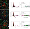 |
Fig. B.1. Left columns: Megacam R and I filter and VIDEO H filter images for each confirmed cluster at z ≥ 0.8 meeting our selection criteria, classified by increasing redshifts. The cyan circles delimit regions within 1 arcmin of the X-ray best fit model centres, which are marked by yellow crosses. The red and brown circles highlight the bright galaxies with a redshift corresponding to the cluster peak redshift ±0.02 and to the cluster redshift ±0.06, respectively. Darker circles indicate the galaxies outside of the central region. The BCGs are circled in white. The X-ray contours in green are logarithmically distributed in ten levels between the maximum and minimum emission observed in a 7 × 7 arcmin2 box around the X-ray source. Middle columns: background subtracted and Gaussian filtered redshift distribution of the bright galaxies within the central arcmin, for the corresponding candidates. The dashed line highlights the median redshift of the highest bin in the redshift spike. Its colour assesses the importance of the overdensity and, therefore, our confidence in the detection: gold for the most reliable candidates (the highest bin height is above 5.5), grey for the reliable one (above 4.5), and beige for the other. Right columns: i − z (0.8 ≤ z < 1.2) or z − J (z ≥ 1.2) CMD plot of the galaxies above the VIDEO 5σ limit within 1 arcmin of the centre. The green squares indicate the galaxies with photometric redshifts that are consistent with the mean redshift plus or minus 1.5 times the standard deviation of the most accurate Gaussian modelling of the redshift spike. The blue lozenges indicate the galaxies with redshifts that are consistent with the sidewings of the most accurate Gaussian model, so up to three times the standard deviation. The deep pink lines indicate the colours predicted by the stellar population model computed in Sect. 4.1. The light pink region is the standard deviation of the difference of this model with method 1 red sequences. |
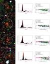 |
Fig. B.1. continued. |
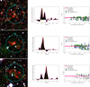 |
Fig. B.1. continued. |
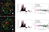 |
Fig. B.2. Left columns: Megacam R and I filter and VIDEO H filter images for the two candidate clusters along the same line-of-sight. Definitions of symbols and contours are given in Fig. B.1. Middle columns: background subtracted and Gaussian filtered redshift distribution of the bright galaxies within the central arcmin for the corresponding candidates. Bottom columns: i − z (0.8 ≤ z < 1.2) or z − J (z ≥ 1.2) CMD plot of the galaxies above the VIDEO 5σ limit within 1 arcmin of the centre. |
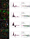 |
Fig. B.3. Left columns: Megacam R and I filter and VIDEO H filter images for the previously detected but unconfirmed candidate clusters at z ≥ 0.8, which are classified by increasing redshifts. The X-ray contours in green are logarithmically distributed in ten levels between the maximum and minimum emission observed in a 7 × 7 arcmin2 box around the X-ray source, except for candidate 6 which displays 25 levels based on a 4 × 4 arcmin2 box. Definitions of symbols are given in Fig. B.1. Middle columns: background subtracted and Gaussian filtered redshift distribution of the bright galaxies within the central arcmin for the corresponding candidates. Bottom columns: i − z (0.8 ≤ z < 1.2) or z − J (z ≥ 1.2) CMD plot of the galaxies above the VIDEO 5σ limit within 1 arcmin of the centre. |
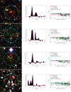 |
Fig. B.3. continued. |
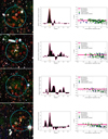 |
Fig. B.4. Left columns: Megacam R and I filter and VIDEO H filter images for the new candidate clusters at z ≥ 0.8, which are classified by increasing redshifts. The X-ray contours in green are logarithmically distributed in ten levels between the maximum and minimum emission observed in a 7 × 7 arcmin2 box around the X-ray source, except for candidate 27 which displays 25 levels based on a 4 × 4 arcmin2 box. Definitions of symbols are given in Fig. B.1. Middle columns: background subtracted and Gaussian filtered redshift distribution of the bright galaxies within the central arcmin for the corresponding candidates. Bottom columns: i − z (0.8 ≤ z < 1.2) or z − J (z ≥ 1.2) CMD plot of the galaxies above the VIDEO 5σ limit within 1 arcmin of the centre. |
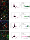 |
Fig. B.4. continued. |
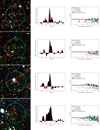 |
Fig. B.4. continued. |
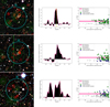 |
Fig. B.4. continued. |
All Tables
All Figures
|
Fig. 1. VIDEO footprints overlaid on XXL-N exposure map. VIDEO covers eight VISTA footprints, the following three of them are within the XXL-N field: XMM1, XMM2, and XMM3. The darker part of the exposure map corresponds to the 46 ks exposure of the XMM-SERVS field. The cyan and salmon crosses correspond to the respective locations of the confirmed clusters and candidate clusters in our sample. |
| In the text | |
|
Fig. 2. Visual summary of the cluster identification process. Top left: background subtracted and Gaussian filtered photometric redshift distribution of the bright galaxies within the central arcmin of candidate 14. The dashed line indicates the highest bin in the redshift spike. Top right: i − z CMD plot of the galaxies above the VIDEO 5σ limit within 1 arcmin of the centre. The green squares indicate the galaxies with photometric redshifts that are consistent with the mean redshift plus or minus 1.5 times the standard deviation of the most accurate Gaussian modelling of the redshift spike. The blue lozenges indicate galaxies with redshifts that are consistent with the sidewings of the most accurate Gaussian model, up to three times the standard deviation. The deep pink line indicates where the red sequence should be at this redshift, based on the best fit calculated in Sect. 4.1. The light pink region indicates the uncertainty on this red-sequence model, which is also calculated in Sect. 4.1. Bottom panel: example of a Megacam r and i filter as well as a VIDEO H filter image for candidate 14, which is one of our candidate clusters. The cyan circle delimits the region within 1 arcmin of the X-ray best fit model centre, which is marked by a yellow cross. The red and brown circles highlight the bright galaxies with a redshift corresponding to the cluster photometric peak redshift ±0.02 and to the cluster redshift ±0.06, respectively. Darker circles indicate the galaxies outside the central region. The BCG is circled in white. The X-ray contours in green are logarithmically distributed in ten levels between the maximum and minimum emission observed in a 7 × 7 arcmin2 box around the X-ray source. |
| In the text | |
|
Fig. 3. Histogram of the candidate cluster redshifts. The black bars correspond to the spectroscopic redshifts of the confirmed clusters and the green bars represent the photometric redshifts of the candidate clusters, which were either previously observed (dark green) or newly detected (lighter green). |
| In the text | |
|
Fig. 4. Comparison between the spectroscopic redshifts of confirmed clusters within the XXL-N/VIDEO overlap and the corresponding photometric overdensities in the VIDEO catalogue. The error bars correspond to the standard deviation of the Gaussian model that fits the photometric spike best. All clusters, except two (not included), were detected in optical. The green dots are the clusters that are a part of our sample, while the blue squares are not included in our sample since they do not meet our X-ray selection criteria. The magenta diamond is the newly confirmed candidate 3. The dashed line represents the ideal case, where zphot = zspec. |
| In the text | |
|
Fig. 5. Illustration of two steps of the first method. Left panels: i − z colour histograms in two fields-of-view (candidate 13 and candidate 8) where the default background (pink line) is either too high or too low. The adjusted background is overplotted in green. Middle panels: resulting colour distribution is the background is left unadjusted. For comparison purposes, the Gaussian models of the red sequence and the blue cloud are shown in pink and blue, respectively; although, they were computed with an adjusted background. The mauve dash-dotted line is the “boundary” used in method 2, 3, and 4. Right panels: colour distribution once the background was adjusted. |
| In the text | |
|
Fig. 6. Fraction of quenched galaxies as a function of the redshift, according to method 4, for each VIDEO candidate, excluding candidates 1, 4, 10, 21, and 24 and the candidate clusters above z = 1.4. Spectroscopically confirmed clusters are indicated by squares, and circles are used to show the other ones. The error bars are the propagation on the Poissonian uncertainties on the integrals of the red sequence and the blue cloud models. |
| In the text | |
|
Fig. 7. Comparison between the quenched fractions obtained by methods 1 and 2 (left panel), methods 1 and 3 (middle panel), or methods 1 and 4 (right panel). The error bars are based on the Poissonian uncertainties on the number of quenched galaxies in the cluster and on the number of galaxies in the considered field-of-view. The background uncertainty included is estimated to 5% of the unscaled background subtraction since we adjusted the subtracted background by steps of 10%. Clusters that have quenching ratios above or below 1.5 times the standard deviation of |
| In the text | |
|
Fig. 8. Top row: mean quenched fraction for each distance bin, for the low quenching (left) and high quenching (right) candidate clusters. Symbols mark the mean quenched fraction, while the shaded regions represent the bin size (x axis) and the standard deviation (y axis) of the quenched fraction. Bottom row: mean quenched fraction for each luminosity bin according to method 2/4 (method 2 is equivalent to method 4 in this context). Luminosities are expressed in terms of L*. We stress that L*, the absolute magnitude, changes with the redshift to reflect the passive evolution of a quenched galaxy. In the interval 0.8 ≤ z < 1.4, the absolute magnitude M* varies from −22.87 to −23.14 in the Ks band and the corresponding stellar masses from 1.45 × 10¹¹ M⊙ to 1.47 × 10¹¹ M⊙. Again, clusters are divided into low quenching (left) and a high quenching (right) groups. These plots only include clusters below z = 1.4 in order to mitigate the selection effects of the catalogue 5σ limit. |
| In the text | |
|
Fig. 9. Best fits for different sub-samples. In each case, three fits were tested: a simple model, in which the metallicity and the formation redshift, assuming an instantaneous starburst, were allowed to vary; and two other models where an additional parameter was allowed to vary, which is the dust content in one case (green dashed line) or the characteristic timescale of the star formation, assuming an exponentially decreasing star formation rate, instead of an instantaneous starburst (purple dash-dotted line). For comparative purposes, we also display the best fit model of Lidman et al. (2012) and our red sequence fit on two panels (the dotted cyan and dotted magenta lines, respectively; see Sect. 4.1). The shaded region corresponds to the 95% confidence region for the simplest model tested and the darker zone corresponds to the 68% confidence region. Left panel: best fits for all BCGs at 0.8 ≤ z ≤ 1.2, except candidate 10 and three BCGs with known photometric problems. Red galaxies are a part of the red sample and blue galaxies are a part of the blue sample. Middle panel: best fits for the red BCGs sub-sample. Right panel: best fits for the blue sub-sample. |
| In the text | |
|
Fig. 10. Division of the blue and red BCGs based on their colour difference with a reference model; the dashed line represents the limit between the two groups. Left: division based on the Lidman et al. (2012) model. Middle: assessment of our sample bimodality based on the red BCGs best fit. Right: same as the left side, but based on the best fit of blue BCGs. |
| In the text | |
|
Fig. 11. Contour plots for the red and blue BCG sub-samples showing the |
| In the text | |
|
Fig. B.1. Left columns: Megacam R and I filter and VIDEO H filter images for each confirmed cluster at z ≥ 0.8 meeting our selection criteria, classified by increasing redshifts. The cyan circles delimit regions within 1 arcmin of the X-ray best fit model centres, which are marked by yellow crosses. The red and brown circles highlight the bright galaxies with a redshift corresponding to the cluster peak redshift ±0.02 and to the cluster redshift ±0.06, respectively. Darker circles indicate the galaxies outside of the central region. The BCGs are circled in white. The X-ray contours in green are logarithmically distributed in ten levels between the maximum and minimum emission observed in a 7 × 7 arcmin2 box around the X-ray source. Middle columns: background subtracted and Gaussian filtered redshift distribution of the bright galaxies within the central arcmin, for the corresponding candidates. The dashed line highlights the median redshift of the highest bin in the redshift spike. Its colour assesses the importance of the overdensity and, therefore, our confidence in the detection: gold for the most reliable candidates (the highest bin height is above 5.5), grey for the reliable one (above 4.5), and beige for the other. Right columns: i − z (0.8 ≤ z < 1.2) or z − J (z ≥ 1.2) CMD plot of the galaxies above the VIDEO 5σ limit within 1 arcmin of the centre. The green squares indicate the galaxies with photometric redshifts that are consistent with the mean redshift plus or minus 1.5 times the standard deviation of the most accurate Gaussian modelling of the redshift spike. The blue lozenges indicate the galaxies with redshifts that are consistent with the sidewings of the most accurate Gaussian model, so up to three times the standard deviation. The deep pink lines indicate the colours predicted by the stellar population model computed in Sect. 4.1. The light pink region is the standard deviation of the difference of this model with method 1 red sequences. |
| In the text | |
|
Fig. B.1. continued. |
| In the text | |
|
Fig. B.1. continued. |
| In the text | |
|
Fig. B.2. Left columns: Megacam R and I filter and VIDEO H filter images for the two candidate clusters along the same line-of-sight. Definitions of symbols and contours are given in Fig. B.1. Middle columns: background subtracted and Gaussian filtered redshift distribution of the bright galaxies within the central arcmin for the corresponding candidates. Bottom columns: i − z (0.8 ≤ z < 1.2) or z − J (z ≥ 1.2) CMD plot of the galaxies above the VIDEO 5σ limit within 1 arcmin of the centre. |
| In the text | |
|
Fig. B.3. Left columns: Megacam R and I filter and VIDEO H filter images for the previously detected but unconfirmed candidate clusters at z ≥ 0.8, which are classified by increasing redshifts. The X-ray contours in green are logarithmically distributed in ten levels between the maximum and minimum emission observed in a 7 × 7 arcmin2 box around the X-ray source, except for candidate 6 which displays 25 levels based on a 4 × 4 arcmin2 box. Definitions of symbols are given in Fig. B.1. Middle columns: background subtracted and Gaussian filtered redshift distribution of the bright galaxies within the central arcmin for the corresponding candidates. Bottom columns: i − z (0.8 ≤ z < 1.2) or z − J (z ≥ 1.2) CMD plot of the galaxies above the VIDEO 5σ limit within 1 arcmin of the centre. |
| In the text | |
|
Fig. B.3. continued. |
| In the text | |
|
Fig. B.4. Left columns: Megacam R and I filter and VIDEO H filter images for the new candidate clusters at z ≥ 0.8, which are classified by increasing redshifts. The X-ray contours in green are logarithmically distributed in ten levels between the maximum and minimum emission observed in a 7 × 7 arcmin2 box around the X-ray source, except for candidate 27 which displays 25 levels based on a 4 × 4 arcmin2 box. Definitions of symbols are given in Fig. B.1. Middle columns: background subtracted and Gaussian filtered redshift distribution of the bright galaxies within the central arcmin for the corresponding candidates. Bottom columns: i − z (0.8 ≤ z < 1.2) or z − J (z ≥ 1.2) CMD plot of the galaxies above the VIDEO 5σ limit within 1 arcmin of the centre. |
| In the text | |
|
Fig. B.4. continued. |
| In the text | |
|
Fig. B.4. continued. |
| In the text | |
|
Fig. B.4. continued. |
| In the text | |
Current usage metrics show cumulative count of Article Views (full-text article views including HTML views, PDF and ePub downloads, according to the available data) and Abstracts Views on Vision4Press platform.
Data correspond to usage on the plateform after 2015. The current usage metrics is available 48-96 hours after online publication and is updated daily on week days.
Initial download of the metrics may take a while.