| Issue |
A&A
Volume 642, October 2020
|
|
|---|---|---|
| Article Number | A131 | |
| Number of page(s) | 11 | |
| Section | Cosmology (including clusters of galaxies) | |
| DOI | https://doi.org/10.1051/0004-6361/202038558 | |
| Published online | 13 October 2020 | |
Infall of galaxies onto groups
1
Instituto de Astronomía Teórica y Experimental (IATE), CONICET-UNC, Laprida 854, X5000BGR Córdoba, Argentina
2
Observatorio Astronómico de Córdoba (OAC), Universidad Nacional de Córdoba (UNC), Córdoba, Argentina
e-mail: This email address is being protected from spambots. You need JavaScript enabled to view it.
Received:
2
June
2020
Accepted:
30
June
2020
Abstract
Context. The growth of the structure within the Universe manifests in the form of accretion flows of galaxies onto groups and clusters. Thus, the present-day properties of groups and their member galaxies are influenced by the characteristics of this continuous infall pattern. Several works both theoretical (in numerical simulations) and observational, have studied this process and provided useful steps for a better understanding of galaxy systems and their evolution.
Aims. We aim to explore the streaming flow of galaxies onto groups using observational peculiar velocity data. The effects of distance uncertainties are also analyzed, as well as the relation between the infall pattern and the group and environment properties.
Methods. This work deals with the analysis of peculiar velocity data and their projection in the direction of group centers, in order to determine the mean galaxy infall flow. We applied this analysis to the galaxies and groups extracted from the Cosmicflows–3 catalog. We also used mock catalogs derived from numerical simulations to explore the effects of distance uncertainties on the derivation of the galaxy velocity flow onto groups.
Results. We determine the infalling velocity field onto galaxy groups with cz < 0.033 using peculiar velocity data. We measured the mean infall velocity onto group samples of different mass ranges, and also explored the impact of the environment where the group resides. Far beyond the group virial radius, the surrounding large-scale galaxy overdensity may impose additional infalling streaming amplitudes in the range of 200−400 km s−1. Also, we find that groups in samples with a well-controlled galaxy density environment show an infalling velocity amplitude that increases with group mass, consistent with the predictions of the linear model. These results from observational data are in excellent agreement with those derived from the mock catalogs.
Key words: techniques: radial velocities / galaxies: clusters: general / large-scale structure of Universe
© ESO 2020
1. Introduction
In the nearby Universe, galaxy peculiar velocities manifest the evolution of the large-scale structure. This structural growth, within hierarchical clustering scenarios, causes the increase of the masses of galaxy groups and clusters through the continuous accretion of smaller systems. Thus, the galaxy velocity field of the infalling regions of clusters is expected to contain a significant radial infall component superposed to other orbits with larger angular momentum content.
The spherical infall model (Regos & Geller 1989) describes the dynamical behavior of objects surrounding isotropic overdense regions with a collapsing velocity field whose amplitude depends on the distance (r) to the local overdensity (Diaferio & Geller 1997). Peebles (1976, 1980) derived a linear approximation to the velocity field induced by an isotropic mass overdensity (δ), and the predicted infall velocity is  δ(r), where Ω0 is the density parameter and H0 is the Hubble constant at present. However, a pure spherical infall model cannot correctly predict the amplitude of the velocity field, since in this model the amplitude of the velocity field depends on local conditions and not on the surrounding mass distribution.
Peculiar velocities arise through galaxy motions departing from a pure Hubble flow induced by the gravitational potential of mass overdensities distributed at large scales, meaning that global conditions are needed to fully describe the velocity field around a mass concentration.
Observationally, the effects of peculiar motions can be reliably inferred statistically via redshift-space distortion (hereafter RSD) studies (Croft et al. 1999; Padilla et al. 2001; Ceccarelli et al. 2006; Paz et al. 2013; Cai et al. 2016). Besides this, peculiar velocities can also be measured directly and used in other ways to extract useful information on the dynamics of galaxies and galaxy systems.
It is important to remember that peculiar velocity measurements directly trace the mass distribution, avoiding the complications of galaxy bias, which is present in RSD (Desjacques & Sheth 2010). These measurements comprise a large range of scales and may also be used to add information regarding the nature of gravity by comparison to other modelings of galaxy motions.
For the aforementioned reasons, the evolution of large structures can be constrained either by direct measurements of peculiar velocities, or by the effects of redshift space distortions. Galaxy peculiar velocities generated by mass irregularities are superimposed to the cosmological expansion so that it can be easily inferred from its redshift and a redshift-independent distance estimation.
Along these lines, galaxy peculiar velocities are attracting interest as promising cosmological probes that provide new information on the dynamics of galaxies and systems at low redshift (Johnson et al. 2014; Huterer et al. 2017; Dupuy et al. 2019; Adams & Blake 2020; Kim & Linder 2020). Tonegawa et al. (2020) analyze redshift–space distortions in clustering measures to constrain cosmological parameters and examine the satellite velocity bias between galaxies and dark matter inside haloes. Recent works reconstruct peculiar velocities and the associated density fields using Cosmicflows-3 data. Their results highlight the ability of peculiar velocities to probe the mass distribution and reveal underdense/overdense structures in the Local Universe (Graziani et al. 2019).
Several authors have performed studies of the streaming motions on large and intermediate scales using peculiar velocities (in regions that extend up to ≈100 h−1 Mpc). In these studies, the bulk flow amplitude derived form the observational velocity field is often compared to the predictions of the standard Λ CDM cosmological model (Watkins et al. 2009; Lavaux et al. 2010; Feldman et al. 2010; Colin et al. 2011; Nusser & Davis 2011; Turnbull et al. 2012; Ma & Pan 2014).
For this work, we studied the accretion of galaxies onto groups using the peculiar velocity field derived from redshift–independent distance measurements, and analyzed the infall amplitude dependence on mass-group and surrounding galaxy-density environments. We also analyzed the effects of anisotropies of the large-scale galaxy distribution on the infall velocity fields onto groups.
This paper is organized as follows: in Sect. 2, we introduce the data sets used; in Sect. 3, we describe the statistical method implemented to obtain the mean infall amplitude from observational peculiar velocities. In Sect. 4, we display and analyze our results regarding infall onto groups using simulated and observational data, respectively. In Sect. 5, we assess anisotropies on infall velocities. In Sect. 6, we examine local effects vs large-scale environments on infall. Finally, in Sect. 7 we summarize and discuss our results.
2. Data
2.1. Observational data
The Cosmicflows–3 catalog (CF3) comprises almost 18.000 distances of galaxies and is the largest compilation of redshift-independent extragalactic distances available (Tully et al. 2016). This catalog is based on the two previous versions, providing distances derived by the authors own observations, as well as estimates extracted from the literature, homogenized to the same scale system. Galaxy distances provided in the catalog were obtained from different methods, for example, the luminosity–linewidth (Tully–Fisher) relation, the fundamental plane (FP), surface-brightness fluctuations, Type Ia supernova (SNIa) observations, etc. Nearby galaxy distances are accurate on a level of 5−10%. However, at greater distances, the uncertainties raise up to 20−25%.
In this work, we used the online version of the CF3 consisting of data for groups of galaxies as well as individual galaxies with no association to groups. While the catalog includes groups identified over the full redshift range of the 2MRS survey (Huchra et al. 2012), following the advice in Tully et al. (2016), we only considered the groups with velocities between 3000 and 10 000 km−1, since the properties of the nearest and farthest groups are uncertain. It is worth mentioning that a group can have multiple contributions, and therefore their distance uncertainties are reduced by averaging over all data sources.
The group catalog also includes masses estimated from the virial theorem and derived from the integrated Ks band luminosity (Tully 2015). It is well known that applying the virial theorem provides a poor estimate of group masses when these systems have a low number of members, while estimates of group masses through their total luminosities may provide more suitable proxies to the actual masses (see Eke et al. 2004). In addition, we highlight that only groups with at least five members have mass estimates derived from the virial theorem. For this reason, we use mass estimates derived from the integrated Ks-band luminosity throughout the paper. In Fig. 1, we display the sky distribution of high- and low-mass groups, according to the median group mass value (red and blue circles for M > 3.4 × 10¹³ M⊙ and M < 3.4 × 10¹³ M⊙, respectively). As can be noticed, both distributions trace large-scale structures in a similar fashion. Further details of the group catalog can be found on Tully (2015) and Tully et al. (2016).
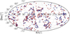 |
Fig. 1. Sky distribution of galaxy groups in equatorial coordinates. Color codes correspond to high/low mass groups, M > 3.4 × 10¹³ M⊙ (red circles), and M < 3.4 × 10¹³ M⊙ (blue circles), respectively. |
The CF3 provides measurements of redshifts and distance moduli so that galaxy peculiar velocities not explicitly included may be derived through:
 (1)
(1)
where vmod is the velocity with respect to the cosmic microwave background (CMB) corrected for cosmological effects (Tully et al. 2013). The calibration of CF3 distances is set by the choice of the fiducial value of H0 = 75 km s−1. Tully et al. (2016) showed that this value minimizes the monopole term with CF3 distances and results in a small global radial infall and outflow in the peculiar velocity field. For these reasons, we used this value in our analysis.
As it is well known, due to observational uncertainties that increase with distance, peculiar velocities can take unrealistic values. This is why we removed galaxies with relative distance errors larger than 20% and peculiar velocities larger than 1500 km s−1 (|vpec| > 1500 km s−1) from our analysis.
With these restrictions, the samples considered in this work comprise 2180 galaxies and 657 galaxy groups. This sample extracted from the CF3 is hereafter referred to as CF3S. In Table 1, we summarize the galaxy and group samples used here and their main characteristics. The first two lines correspond to the CF3S galaxy and group samples previously described. The subsequent lines contain information on the group subsamples selected for the analyses carried out in this work and are introduced in the corresponding sections.
Summary of the main characteristics of groups and galaxy samples.
2.2. Mock catalogs
In order to compare model predictions to observational results, we used mock catalogs based on galaxies extracted from the semi-analytical model presented by Henriques et al. (2015). This catalog includes 2MASS photometric bands, which are also in the group catalog supplement in CF3. This semi–analytical model is an update of the Munich galaxy formation model, consistent with the first–year Planck cosmology (Planck Collaboration I 2011), including a new treatment of baryonic processes to reproduce recent data on the abundance and passive fractions of galaxies from z = 3 down to z = 0. Henriques et al. (2015) used the Millennium simulation (Springel et al. 2005), which follows structure formation in a 500 h−1 Mpc-sized box, comoving with a resolution limit of 8.6 × 10⁸ h−1 M⊙. The cosmological parameters used in this semi-analytical model correspond to the first–year Planck, σ8 = 0.829, H0 = 67.3 km s−1 Mpc−1, ΩΛ = 0.685, Ωm = 0.315, Ωb = 0.0487.
We constructed 25 mock catalogs in order to compare model predictions to observational results and examine possible biases generated by systematic errors in the observational data. Each of these mock catalogs has a Hubble parameter of H0 = 75 km s−1, consistent with the Cosmicflows–3 catalog, and are used to estimate the effect of cosmic variance on our results. The set of mocks mimic (as much as possible) the characteristics of the observational catalogs. In order to reproduce the statistical properties of the observations, we placed an observer inside the simulation box and considered a volume representative of the observational volume. The same angular mask as the observational catalog was applied, excluding an area similar to that produced by the extinction of our galaxy’s disk (zone of avoidance). The galaxies are selected at random so as to obtain comparable number densities of galaxies with a similar redshift distributions. In addition, the mock catalogs are also designed to reproduce the current observational measured distances and their estimated uncertainties.
We used haloes identified using a friends of friends (FoF) algorithm with standard parameters (Henriques et al. 2015). We selected the FoF halos imposing a similar mass distribution to the observations. These restrictions provide suitable samples to test the dynamics of infalling semianalytic galaxies onto these mass inhomogeneities, resembling the infall of galaxies onto groups in the real universe.
Large uncertainties of distance measurements strongly affect the derived radial peculiar velocities and uncertainties can be as large as the peculiar velocities. In addition, distance estimates are subject to systematic biases, as homogeneous and inhomogeneous Malmquist biases (Strauss & Willick 1995; Dekel 1994), which can generate spurious artifacts in the inferred velocity field.
We analyzed and quantified the impact of uncertainties of distance measures on the infall mean velocity determination by assigning errors to the mock catalogs similar to those affecting the observational data In general, the different distance indicators have a fractional distance uncertainty. Primary distance estimators such as the tip of the giant branch, cepheids, or surface brightness fluctuations give distances with relative errors ranging from 5%−10%, whereas secondary indicators reach uncertainty estimates up to 25%.
As it is well known, uncertainties in redshift-independent galaxy distance estimates are consistent with a Gaussian distribution in distance moduli. As a consequence of this behavior, uncertainties of both distance and peculiar velocity are expected to have a log-normal distribution. In order to asses the effects of these distance uncertainties on our results, we assumed a Gaussian distribution of errors in distance moduli, with the mean and dispersion as derived from the CF3, that is to say, consistent with a mean relative-distance uncertainty of 17%. These uncertainties are used to modify the distances of each galaxy in the mock catalog dn = d × 10fd, where fd is taken from a Gaussian distribution. These mock catalogs are hereafter referred to as the biased mock catalogs, while mock catalogs with no errors in galaxy distances are referred to as the unbiased mock catalogs.
The left panel of Fig. 2 displays the distance distribution for both the CF3S and for a typical random mock with modified distances (biased mock). As it can be seen in this figure, both distributions are similar, providing confidence that our assumptions assigned accurate distance uncertainties in simulated data. The radial peculiar velocities computed from Eq. (1) are shown in the right panel. Dashed lines correspond to the CF3S, and dotted-dashed lines correspond to biased mock. In order to highlight how distance errors introduce biases in radial peculiar velocities, in the same panel we show the distribution of the velocities for the same mock with error-free distances (unbiased mock). The distributions of distances associated to CF3S and the biased mock reveal a skewness towards negative peculiar velocities and both are flatter than unbiased mock. This effect is a consequence of the asymmetry in the distribution of fractional errors on distance, skewing peculiar velocity measurements to negative values. Regarding the comparison between distances and peculiar velocities, there is a qualitatively good agreement between CF3S and the biased mock catalog. The galaxies from the biased mock catalog are distributed consistently with observations.
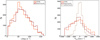 |
Fig. 2. Left panel: distributions of distances in CF3S (solid orange line) and in a typical mock catalog with distance errors included (biased mock, dashed brown line). Right panel: distribution of radial peculiar velocities in CF3S (solid line histogram) and in the biased mock catalog (dashed histogram). A large tail toward negative values is observed in both distributions. The distribution associated to the mock catalog without errors (unbiased mock, dotted brown line histogram) has a nearly Gaussian radial peculiar velocity distribution. |
3. A statistical approach to derive the mean infall component of galaxy peculiar velocities onto groups
3.1. Statistical method
From the dynamical point of view, galaxy groups can be idealized as spherical, isolated mass overdensities. Under this simplified approximation, the expected peculiar velocity field of galaxies in groups and in their surroundings results from the sum of a spherical infall component plus a random velocity dispersion induced by the virialization of the central region. This picture is consistent with linear theory, where convergent velocity fields may be directly associated to spherical, isolated-mass overdensities in a cosmological substratum. Given the limitations of the observations where only the line–of–sight (LoS) projection of the peculiar velocity of galaxies can be estimated, the derivation of the observed velocity field associated to the infall onto groups depends on the position of the galaxy relative to both the group center and the observer (see Eq. (2)). Then, for galaxies at a relative distance r to the group, the infall amplitude (Vinf(r)) can be derived from the LoS peculiar velocity (Vpr) by the lineal relation shown in Eq. (2):
 (2)
(2)
where θ is the angular separation between the galaxy, and the observer is as seen from the group center.
In order to derive Vinf(r), we considered galaxies located at different spherical concentric shells of radius r around the groups. For each shell, we examined the dependence of the peculiar velocity on cos(θ). Then, for different cos(θ) bins, we calculated the average galaxy peculiar velocity ⟨Vpr⟩, iteratively removing the galaxies of which the peculiar velocity lies at more than 1.5σVpr from the mean derived for each bin with the data used in the previous iteration. The mean infall amplitude Vinf(r) can be simply derived by applying a least-squares linear fit to the (cos(θ), ⟨Vpr⟩) vs group–centric radius r.
We note that in the reference system adopted, positive velocities correspond to infall motions while outflow velocities have negative values in our convention.
3.2. Recovering the mean infall amplitude in simulated data
The comparison between the mean infall amplitudes as a function of r obtained by averaging the peculiar velocities and those derived form Eq. (2) allows for a reliability test of our methods. To this aim, we took advantage of the information provided by synthetic catalogs, in particular the three-dimensional and the LoS peculiar velocities.
We explored the dependence of the peculiar velocity on cos(θ) in the unbiased mock catalogs and applied a least-squares linear fit to (cos(θ),⟨Vpr⟩). We show some examples of this relation in the four panels on the left of Fig. 3, where each panel corresponds to a different group-centric distance range, as indicated in the figure, where the slopes of the linear fits are displayed in the small upper boxes in each panel. These slopes correspond to the derived mean infall amplitudes and are used to generate the infall curve shown in the right panel of this figure.
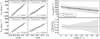 |
Fig. 3. Left figure: mean peculiar velocity as a function of the angle the galaxy-group and group-observer directions (Θ) in the unbiased mock catalogs. Each panel corresponds to a different galaxy-group distance, as is indicated in the figure. The dashed line indicates the best linear fitting, the slope is associated with the infall amplitude (Vunbiased mock) and it is specified in each panel. The gray region corresponds to the peculiar velocity dispersion. Right figure, upper panel: mean infall velocity as a function of distance to the group center in the unbiased mock catalogs. The solid line indicates the mean velocity directly obtained from the three-dimensional peculiar velocity (Vunbiased mock (3d)). Dashed line corresponds to the infall amplitude (Vunbiased mock) obtained by applying our statistical method at LoS peculiar velocities and coincides with the slopes of the lines in the left figure. The displayed velocities are averaged over 25 unbiased mock catalogs and the shadow region shows their dispersion. Right figure, lower panel: dispersion of the ratio between the mean infall velocities (Vunbiased mock (3d)) and the mean infall (Vunbiased mock) velocities for each unbiased mock. |
We derived the mean infall amplitude Vinf(r) as a function of distance to the group for the 25 mock catalogs, and in the upper-right panel of Fig. 3, we show the results averaged over the 25 unbiased mock catalogs. The solid line denotes the mean infall motion derived from the projection of the three–dimensional velocity vector (Vunbiased mock (3d)) along the group-centric direction, whereas the dashed line corresponds to the mean infall velocity (Vunbiased mock) inferred by the procedure described in Sect. 3 and shown in the left panels.
Uncertainties are derived from the scatter of measurements obtained from the 25 unbiased mock catalogs, consistent with a suitable measure of cosmic variance.
As it can be seen in the upper-right panel of Fig. 3, the mean infall velocity estimated via the three–dimensional vector (solid line) and those inferred from LoS peculiar velocities (dashed line) are in excellent agreement, indicating that the proposed statistical method allows us to derive the mean infall velocities from peculiar velocities.
We notice a convergent velocity field onto groups that can be clearly distinguished up to group-centric distances of 18 Mpc h−1, showing large-scale flows of galaxies directed onto groups.
Closer to group centres, the mean infall velocity reaches a maximum of approximately 200 km s−1, where the effects of the potential well associated with the groups dominates the local radial infall. At larger distances, the velocity field is no longer dominated by the group mass concentration, but instead obeys the surrounding large-scale structure, implying an average decline of the mean infall velocity.
The shaded region in the lower-right panel of Fig. 3 shows the dispersion of the ratio between the actual mean group-centric infall velocity and the mean infall velocities derived from peculiar velocities for each unbiased mock. As we can see, there is a suitable agreement between the two measures, which proves the reliability of our method in deriving infall amplitude determinations.
4. Observed velocity field around groups
Once we tested the reliability of our methods to assess the effects of LoS projection of peculiar velocity in the unbiased mock catalogs, we studied the streaming infall flow around groups. To this aim, we used observed peculiar velocity data, applying our analysis to the samples of galaxies and groups described in Sect. 2.
We derived the mean streaming velocity toward groups in the observational data by applying the same procedures used in the unbiased mock catalogs (Sect. 3.2). In Fig. 4, we show the mean projected peculiar velocity as a function of cos(θ) bins for the samples of galaxies and groups taken from the CF3S (points) and their best linear fitting (dashed lines). The different panels correspond to spherical shells at different distances (r) to the groups, as indicated in the figure. In this figure, uncertainties are derived from the scatter of measurements obtained from the CF3S (error bars), and gray shadow regions correspond to the dispersion of results obtained in 25 biased mock catalogs. We acknowledge the very good agreement between the results of the biased mock catalogs and the observations, which is totally consistent within uncertainties.
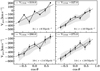 |
Fig. 4. Mean peculiar velocity as a function of the angle between the galaxy-group and group-observer (θ) directions in the CF3S (points). Each panel corresponds to a different galaxy-group distance, as is indicated in the figure. The dashed line indicates the best linear fitting, the slope is associated to the infall amplitude (VCF3S) and it is specified in each panel. The error bars correspond to the peculiar velocity dispersion. The gray shaded areas enclose the dispersion of mean peculiar velocity from the 25 biased mock catalogs. We note that the range of the y-axis in upper and lower panels is different. |
As can be seen, we obtain positive slopes consistent with a neat infall (see the small panels in the right of the figure) for all the distance ranges analyzed. Thus, our results clearly signal infall onto groups. Moreover, inspection of this figure reveals that the dispersion around the mean infall velocity is larger in the inner group-centric distance bin (upper left panel of Fig. 4) possibly due to the contribution of motions from the virialized and pre-virialized regions (Diaferio & Geller 1997; Diaferio 1999). Beyond this scale, the mean projected peculiar velocity becomes more stable and errors get smaller, showing the expected smoother flow from large distances. At larger scales, the influence of surrounding structures starts to affect the infall pattern, and the systematic, radially inward velocities decrease. This behavior is expected at large scales, where the infall signal becomes negligible due to the presence of the gravitational pull of neighboring groups, clusters, and filaments (we note the different peculiar velocity ranges of the upper and lower panels).
This behavior could be a consequence of biases that affect CF3S distances resulting in spurious velocity flows (Tully et al. 2016). Furthermore, the radial peculiar velocity distribution has a negative skewness, as shown in Fig. 2, and this asymmetric bias could contribute to us obtaining large negative peculiar velocities. It is worth noting that the biased mock catalogs present the same behavior (gray shaded areas), while unbiased mock ones do not show this trend.
In Fig. 5, we show the resulting mean velocity infall as a function of group-centric distance, Vinfall(r) for CF3S, (VCF3S, dot-dashed lines), as derived from the linear fit applied to each panel of Fig. 4. We also show, in this figure, the results from mock LoS peculiar velocities with (Vbiased mock) and without (Vunbiased mock) errors included (dashed and solid lines, respectively).
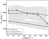 |
Fig. 5. Mean infall velocity as a function of distance to the group center for biased samples. Dashed line indicates the mean velocity obtained from the mock with errors included (biased mock), and the dot-dashed line corresponds to the Cosmicflows-3 sample (CF3S). For comparison, we include the mean infall velocity for the unbiased mock(solid line). Error bars correspond to the uncertainty in the mean infall velocities from CF3S. The shaded region indicates the variance obtained from 25 mocks without (with) errors included in the catalog realizations. |
It can be seen that when distance uncertainties are included, the mean infall velocity corresponding to the biased mock catalogs agrees well with those derived from CF3S data (dot-dashed and dashed lines, respectively). Upon inspection of Fig. 5, it is clear that VCF3S infall flow (dashed line) reaches a maximum of approximately 300 km s−1, which is 50% higher when compared to the infall flow from the unbiased mock catalogs (solid line).
As is evident from this analysis, it is crucial to properly address distance uncertainties to derive reliable peculiar velocity fields around groups.
4.1. Correcting for distance uncertainty effects on infall determination
The resulting average group-centric infall velocities recovered from the mock catalogs are used to calibrate and correct the observational results.
In order to correct for the effect of distance uncertainties in the inferred infall velocities, we compared the results from the mock catalogs with and without the inclusion of errors (biased mock and unbiased mock, respectively). We calculated the ratio f = Vbiased mock/Vunbiased mock, where Vbiased mock is the infall amplitude of the mock catalogs with distance errors (see dashed line in Fig. 5), and Vunbiased mock is the infall amplitude from the mock catalogs without distance uncertainties (see solid lines in Fig. 5).
A fitting function of the form f = ar2 + br + c is sufficient to provide a good description of the observed-to-actual-velocity ratio. We find that the parameters a = 1.2, b = 0.05, yc = −0.0002 provide a good fit to the measured values of f for this group sample. The fitting parameters obtained for different subsamples provide the factors (f) used to correct the infall velocities measured (VCF3S) in the corresponding CF3S. These observational flows corrected hereafter are called Vcorrected CF3S, in a similar way, flows corrected on the biased mock catalogs are called Vcorrected mock flows. The corrected infall pattern derived from the CF3S is shown as dot-dashed lines in Fig. 6, the dashed line corresponds to the average infall flow in 25 corrected mock catalogs, and the solid line corresponds to the actual mean infall flow directly obtained from peculiar velocities in unbiased mock catalogs. The gray region encloses the fifth and ninety-fifth percentiles of the infall distribution on the 25 corrected mock catalogs, which can be taken as a measure of cosmic variance.
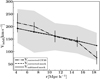 |
Fig. 6. Mean infall velocity as a function of distance to the group center for corrected samples. The dashed lines indicate the mean velocity obtained from the corrected mock catalogs, and the dot–dashed line corresponds to Cosmicflows–3 sample corrected (corrected CF3S). The solid lines correspond to the mean infall velocity for the unbiased mock catalogs shown in solid lines on Fig. 5. Error bars correspond to the uncertainty in the Vcorrected CF3S. The shaded regions indicate the variance obtained from the 25 corrected mock catalogs. |
As can be seen in Fig. 6, there is clear evidence of infall motions up to 16 Mpc h−1. We also notice that Vcorrected CF3S and Vcorrected mock reaches 200 km s−1 at regions close to the groups (≈4 Mpc h−1). The resulting mean velocities obtained here are consistent with those found by Ceccarelli et al. (2005). For greater distances to the groups, the infall amplitude decreases down to about 120 km s−1 and infall uncertainties increase.
Here and throughout, we used the Kolmogorov–Smirnov (KS) test to find the statistical significance of the differences between infall velocity amplitudes for the different samples. We consider that the differences between distributions are highly significant if the p-value is p < 0.011. The KS test confirms that the slope value of Vcorrected CF3S profile in Fig. 6 is significant at the 3σ level.
These results are reasonable considering that close to the groups, galaxy peculiar velocities are dominated by the group potential, whereas at larger distances the surrounding large-scale structure strongly affects the velocity field.
Taking into account our cosmic variance determinations, the Vcorrected CF3S mean infall velocities are consistent with the Vcorrected mock ones from the biased mock catalogs.
4.2. Dependencies on group properties
In this subsection, we analyze the characteristics of the peculiar velocity field around groups and its relation to group mass. We subdivided the group sample according to mass estimated from the integrated Ks-band luminosity (hereafter mass, M) into two group subsamples: groups with M > 3.4 × 10¹³ M⊙, and M < 3.4 × 10¹³ M⊙, dubbed high-mass (HM) and low-mass groups (LM), respectively. This limit was chosen in such way that each subsample contains a similar number of groups, as shown in Table 1.
Similarly, we analyzed the 25 mock catalogs and estimated the mean infall amplitude for galaxies in the unbiased mock and biased mock catalogs. This allowed us to infer the correction factors (f) for each subsample and use them to derive the true amplitudes of the infall velocity field in the observations. Here and throughout, observed mean infall velocities always refer to those corrected by the factor f in CF3S and the cosmic variance is obtained from the 25 corrected mock catalogs.
The resulting relative amplitude of the radially inward-streaming motions are shown in Fig. 7. We show the ratio ( ) between the infall amplitude of the two samples. As can be seen in this figure, there is a clear difference in the mean infall amplitude onto group samples of high and low masses, the infall velocity amplitude associated with the high-mass groups is systematically larger than that corresponding to the low-mass groups in the range of group centric distances explored. This behavior is stronger close to the center of the groups, where galaxies around high-mass groups exhibit noticeably higher infall than galaxies around low-mass groups. The KS test shows that the differences between infall velocity amplitudes are statistically significant (p < 0.01), consistent with a statistical confidence at the 3σ level. The gray shaded area in this figure corresponds to the cosmic variance taken from the mock catalogs, while error bars indicate the relative uncertainty between both samples as derived from the linear fitting of peculiar velocities and cos(θ).
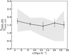 |
Fig. 7. Ratio of the mean infall velocity of high-to-low-mass groups as a function of distance to the group centers in observational data (solid line). Error bars indicate the uncertainty in the mean infall velocity, and the gray shadow region shows the dispersion of 25 mock catalogs. |
Based on these studies, we adopted mass estimated from luminosity as a suitable indicator of group mass.
5. Large-scale environment versus infall
5.1. Velocity field anisotropies
In a first approximation, the mean velocity field around groups of galaxies can be suitably described by the spherical infall model. The velocities predicted by this model are in qualitative agreement with our results (see Fig. 7, where the amplitude of the mean infall velocity field is strongly influenced by the group total mass). This model has also been successful in constraining group masses (Pivato et al. 2006), although we notice relevant departures from this simple picture given that the mass distribution around groups is strongly anisotropic due to the network of filaments, walls, and clusters dominating the large-scale Universe. For this reason, the velocity fields surrounding groups exhibit a significant variance that is strongly connected to surrounding large-scale structures (Kashibadze et al. 2020; Courtois et al. 2019; Tully et al. 2019; Libeskind et al. 2015). These effects have been reported and analyzed in numerical simulations (Ceccarelli et al. 2011), and in this work we aim to obtain observational counterparts of these theoretical results.
We note that since only the LoS components of observational peculiar velocities are available, the observational velocity field for groups with overdensities along the LoS can be strongly determined by galaxies residing in these filamentary regions. On the other hand, groups located in global overdensities perpendicular to the LoS may have galaxies with velocity dominated by flows from underdense regions onto groups. In this section, we examine these different cases by analysing the derived infall flow from overdense/underdense regions by selecting two samples of groups with large-scale surrounding regions parallel and perpendicular to the LoS. In order to perform this test, we computed the density in a spherical region of radius 15 Mpc h−1 centered in the groups and considered the regions close to the LOS,  , and perpendicular to it,
  , separately. This allows us to separate the total subsample into two groups, those with predominant LoS overdensities (∥), and those predominant overdensities in the plane of the sky (⊥). The number of groups for each sample is stated in Table 1.
With the aim of shedding light on the anisotropic infall onto groups in the observations, we estimated the mean velocity field around the two samples of groups. Applying a similar analysis to that performed in the previous subsection, we computed the ratio between both subsamples, and show the results in Fig. 8. It is clear that mean velocities are significantly different, as inferred from the KS test, which gives a high statistical significance above the 5σ level. The Vinfall ∥/Vinfall ⊥ ratio for the two group samples remains below 1 (solid line, Vinfall ⊥ > Vinfall ∥), indicating that the streaming motion of galaxies onto groups with large underdense regions is faster than those of galaxies from global overdensities. This result is in sync with those of Pereyra et al. (2019), Mahajan et al. (2012) and Ceccarelli et al. (2011), which showed that a relatively high galaxy density in the infalling regions of groups promotes tidal interactions with neighboring galaxies, resulting in a smaller magnitude of the velocities along these high-density regions. We stress the fact that both subsamples of groups have similar mass and luminosity distributions, so these differences should be put down to an environmental difference.
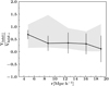 |
Fig. 8. Mean infall velocity ratio (Vinfall ∥/Vinfall ⊥) for groups with overdensities in the direction parallel and perpendicular to the LoS in the observational data. Error bars indicate the uncertainty in the relative mean velocity, and the gray shaded region shows the variance as in previous figures. |
5.2. Overall density around groups
The spherical infall model assumes an isotropic mass distribution of groups as well as their isolation so that infall pattern is associated with an isotropic convergent velocity field. Given that groups of galaxies are not isolated but immersed in the cosmic web, local irregularities can affect the local dynamics, and even more, large-scale bulk motions may imprint significant peculiar velocities on the galaxies beyond the small/intermediate effects associated with the galaxy groups (Kitaura et al. 2012; Hoffman et al. 2018; Graziani et al. 2019).
We analyzed the effects of the surrounding density field around groups on the infalling velocity pattern by selecting three subsamples of groups embedded in underdense, intermediate, and overdense regions. For the environment characterization, we computed the integrated galaxy overdensity in a region from 5 Mpc h−1 to 10 Mpc h−1 (δρe) centered in the group, and we estimated the mean velocities as a function of group-centric distance for each sample. The low-density subsample is defined by 0 < δρe < 2, the intermediate-density subsample by 2 < δρe < 4, and the high-density subsample, by δρe > 4.
In Fig. 9, we show the resulting infall velocity pattern derived from the three group subsamples that consider their mean surrounding density. The solid line corresponds to 0 < δρe < 2, the dashed line to 2 < δρe < 4, and the dot–dashed line to δρe > 4. As you can see in this figure, groups in all density environments show systematic infalling velocities over the entire range of distances explored, with increasing amplitude for higher density environments. In Fig. 9, it can be appreciated that as the density environment around groups increases, the amplitude of the streaming infall velocity field increases as well. The KS tests confirm that the differences among infall velocity amplitudes of high-, intermediate-, and low-density environments are statistically significant at a very high confidence level (> 3σ for all samples). As expected, we find a strong dependence of the velocity field around groups on both group mass and surrounding mass density on significantly large scales (Einasto et al. 2003a, 2005).
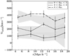 |
Fig. 9. Dependence of infall onto groups from regions with different density environments in observational data. The lines correspond to the mean infalling velocity onto groups embedded in regions with δρe > 4 (dot–dashed), 2 < δρe < 4 (dashed), and 0 < δρe < 2 (solid). The three gray shaded regions represent the variance from equivalent high-, medium-, and low-density environments in the mock catalogs, respectively. Error bars correspond to the uncertainties in the derived mean infalling velocities. |
6. Local versus global velocity fields
Several works (e.g., Einasto et al. 2003a,b, 2005; Lietzen et al. 2012) have shown that groups and clusters of galaxies in high-density regions are richer, more massive, and more luminous than groups and clusters of galaxies in low-density regions. In this context, the results obtained in the previous section could be biased by the inclusion of samples of different mass groups. Therefore, in this section, we examine the inferred mean infall pattern considering the effects of group mass and environment separately.
6.1. Density around groups
We restricted the sample construction so that the groups have comparable statistical mass properties. Given that we selected samples of groups with similar statistical properties, the possible differences in their velocity fields should be associated only with the environment.
We selected three subsamples of groups with similar mass (and luminosity) distributions and embedded in regions of different overall galaxy density bins, where these density bins correspond to those in Sect. 5.2. Since the mass distributions of the three subsamples are similar, we expect similar contributions to the mean infall by the group itself. Therefore, the differences between the resulting velocity field of the two samples can be associated with the difference imposed by the surrounding environment. In Fig. 10, we show the mean infall amplitude as a function of group-centric distance for groups in different galaxy density environments, solid lines 0 < δρe < 2, dashed line 2 < δρe < 4, and dot-dashed line δρe > 4. As you can see in the figure, the velocities are comparable for distances to the group center smaller than ∼6 Mpc h−1 where the infall amplitude rises to Vinfall ≈ 200 km s−1 at r ≈ 6 Mpc h−1. This is consistent with the fact that the three samples have comparable mass distributions. So, the effect of similar group masses on the surrounding velocity field can be clearly appreciated. On the other hand, in Fig. 10 we see that the velocity curves differ significantly at large separations (r > 8 Mpc h−1), with associated KS test p-values < 0.01. These results show the impact of the large-scale environment on the velocity field, which is in agreement with previous works (Einasto et al. 2005; Lietzen et al. 2012).
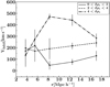 |
Fig. 10. Same as Fig. 9 with observational group subsamples restricted to have a similar mass distribution. The line types correspond to the same environmental density ranges analyzed in Fig. 9. Error bars indicate the uncertainty in the mean infalling velocities. |
6.2. Group mass dependence
Once we examined the effect of the global overdensity on the velocity field around poor galaxy groups, we then explored the contribution of group mass to the velocity field in an environment-controlled subsample We restricted the sample of groups to those residing in global environments within a restricted galaxy overdensity (1 < δρe < 2.5) corresponding to the 25 and 75 percentiles and comprises 50% of the total group sample. Within this constraint, we selected two subsamples of groups with masses larger/smaller than the total sample median mass (≈3.4 × 10¹³ M⊙). The mean/median mass for the larger (smaller) subsample is 10.4 × 10¹³/6.74 × 1013 M⊙ (18.8 × 10¹²/17.8 × 1012 M⊙), with mean/median mass ratios 5.5/3.7.
Given that we select the two subsamples of groups in similar large–scale environments, any differences on the peculiar velocity field should be attribute to the group mass.
We derive the mean infall amplitude for the two subsamples and show the results in Fig. 11, where the solid (dashed) line corresponds to group masses larger (lower) than the median. As we can see in this figure, high- and low-mass groups exhibit mean infall amplitudes clearly distinguishable closer to the group (r < 8 Mpc h−1): the infall amplitude reaches 300 km s−1 for high-mass groups (solid line) and remains bellow 100 km s−1 for low-mass groups (dashed line) at the smallest group-centric distances analyzed (∼4 Mpc h−1). The KS test shows that, up to 8 Mpc h−1, the differences between the infall velocity amplitudes of these samples are statistically significant at the 2.5σ level. Consequently, the infall amplitude ratio of high-mass to low-mass groups is a factor of 4.5 ± 1.0 in this close surroundings of groups, consistent with the mass ratio values (5.5 mean, 3.7 median) of the two group subsamples. This ratio is in very good agreement with the linear infall model predictions for the velocity field. As we can see in Figs. 10 and 11, we can easily distinguish two regimes characterizing the peculiar velocity field on small and large scales.
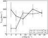 |
Fig. 11. Infall dependence on group mass in the observational data. The group subsamples are restricted to reside in similar density environments (1 < δρe < 2.5). The solid (shaded) line corresponds to high- (low-) mass groups with M larger (smaller) than Mmedian. Error bars represent the uncertainty in the derived mean infalling velocities. |
7. Discussion
Galaxy peculiar velocities originate in departures of motions from a pure Hubble flow induced by irregularities of the mass distribution at large scales. These motions have a statistical imprint on the redshift–space distortions of the two-point correlation function and provide useful information on the global dynamics. However, peculiar velocities can be directly estimated through redshift-independent distance indicators and may be used to extract useful information on the dynamics of galaxies and galaxy systems besides the correlation function analysis. Since peculiar velocity measurements provide a direct trace of the mass distribution, there are no issues regarding galaxy bias, which adds complexity in redshift–space correlation analysis. For this reason, direct estimates of galaxy peculiar velocities may provide a useful cosmological test in forthcoming surveys with more accurate determinations in the Universe. In this work, we focused our analysis on the measurements of infall of galaxies onto groups, and its dependence on group mass and environment. Since groups of galaxies are part of the cosmic web, the local dynamics cannot be simply addressed through a spherical infall model given that large scale bulk motions affect the local effects associated to group mass overdensities.
Firstly, we applied the spherical infall model to derive the mean infall velocity pattern onto groups of different characteristics. Since only the LoS projection of galaxy peculiar velocities can be obtained, the derived infall velocity field relates to galaxy positions relative to both the group center and the observer (see Eq. (2)). Present data are affected by large distance measurement uncertainties which lead to large peculiar velocity errors. This fact is associated with the presence of systematic effects of distance estimates that can bias the inferred velocity field. To properly address the impact of distance measurement uncertainties on the mean infall velocity determination we assign suitable errors to mock catalogs constructed in a similar fashion to the observations.
We obtain accurate determinations of the mean infall velocity profile around groups of different mass ranges and in different environments, which exhibit amplitudes in the range of 200 − 350 km s−1, entirely consistent with numerical simulation results. We extended our work by considering the impact of a large-scale environment on the mean infall galaxy velocity onto groups.
We compared the effects of large-scale inhomogeneities around galaxy groups on the mean infall velocity, finding that the effects are significantly smaller along the direction of high-density enhancement compared to those in the low-density direction. This provides evidence that groups grow in a different fashion from filaments than from elsewhere. These results are in agreement with previous studies of the environmental effects on groups and clusters growing via mass accretion from their surrounding structures, ranging from isolated galaxies to large groups that merge to form larger systems (McGee et al. 2009). McGee et al. (2009) also showed that a large fraction of galaxies accreted onto clusters were formerly in groups.
We obtain a significant dependence of the mean infall pattern on the group large-scale environment consistent with higher infall velocities onto groups residing in large overdense regions.
We recall that infall models are mainly based on assumptions of spherical symmetry onto an isolated mass overdensity. This simplified scenario may have an impact on total group mass determinations, taking into account our studies of the streaming motions dependence on the global density environment and anisotropic mass distribution around groups in observations.
Due to upcoming improvements on observational data and peculiar velocity precision, studies such as that presented in this work may aid our current understanding of the growth of structures in the Universe.
When we quote the statistical significance of a difference between two distributions (xi and yi), we compute P(Δχ2, Nd.o.f.) where Δχ2 = ∑i[di/σ(di)]2 with di = (xi–yi) for each bin and  . We note that P(x, N) is a χ2 distribution with N degrees of freedom.
Acknowledgments
This work has been partially supported by Consejo de Investigaciones Científicas y Técnicas de la República Argentina (CONICET), and the Secretaría de Ciencia y Técnica de la Universidad Nacional de Córdoba (SeCyT).
References
- Adams, C., & Blake, C. 2020, MNRAS, 494, 3275 [CrossRef] [Google Scholar]
- Cai, Y.-C., Taylor, A., Peacock, J. A., & Padilla, N. 2016, MNRAS, 462, 2465 [NASA ADS] [CrossRef] [Google Scholar]
- Ceccarelli, M. L., Valotto, C., Lambas, D. G., et al. 2005, ApJ, 622, 853 [NASA ADS] [CrossRef] [Google Scholar]
- Ceccarelli, L., Padilla, N. D., Valotto, C., & Lambas, D. G. 2006, MNRAS, 373, 1440 [NASA ADS] [CrossRef] [Google Scholar]
- Ceccarelli, L., Paz, D. J., Padilla, N., & Lambas, D. G. 2011, MNRAS, 412, 1778 [CrossRef] [Google Scholar]
- Colin, J., Mohayaee, R., Sarkar, S., & Shafieloo, A. 2011, MNRAS, 414, 264 [NASA ADS] [CrossRef] [Google Scholar]
- Courtois, H. M., Kraan-Korteweg, R. C., Dupuy, A., Graziani, R., & Libeskind, N. I. 2019, MNRAS, 490, L57 [CrossRef] [Google Scholar]
- Croft, R. A. C., Dalton, G. B., & Efstathiou, G. 1999, MNRAS, 305, 547 [NASA ADS] [CrossRef] [Google Scholar]
- Dekel, A. 1994, ARA&A, 32, 371 [NASA ADS] [CrossRef] [MathSciNet] [Google Scholar]
- Desjacques, V., & Sheth, R. K. 2010, Phys. Rev. D, 81, 023526 [NASA ADS] [CrossRef] [Google Scholar]
- Diaferio, A. 1999, MNRAS, 309, 610 [NASA ADS] [CrossRef] [Google Scholar]
- Diaferio, A., & Geller, M. J. 1997, ApJ, 481, 633 [NASA ADS] [CrossRef] [Google Scholar]
- Dupuy, A., Courtois, H. M., & Kubik, B. 2019, MNRAS, 486, 440 [NASA ADS] [CrossRef] [Google Scholar]
- Einasto, M., Einasto, J., Müller, V., Heinämäki, P., & Tucker, D. L. 2003a, A&A, 401, 851 [NASA ADS] [CrossRef] [EDP Sciences] [Google Scholar]
- Einasto, J., Hütsi, G., Einasto, M., et al. 2003b, A&A, 405, 425 [NASA ADS] [CrossRef] [EDP Sciences] [Google Scholar]
- Einasto, J., Tago, E., Einasto, M., et al. 2005, A&A, 439, 45 [NASA ADS] [CrossRef] [EDP Sciences] [Google Scholar]
- Eke, V. R., Frenk, C. S., Baugh, C. M., et al. 2004, MNRAS, 355, 769 [NASA ADS] [CrossRef] [Google Scholar]
- Feldman, H. A., Watkins, R., & Hudson, M. J. 2010, MNRAS, 407, 2328 [NASA ADS] [CrossRef] [Google Scholar]
- Graziani, R., Courtois, H. M., Lavaux, G., et al. 2019, MNRAS, 488, 5438 [CrossRef] [Google Scholar]
- Henriques, B. M. B., White, S. D. M., Thomas, P. A., et al. 2015, MNRAS, 451, 2663 [NASA ADS] [CrossRef] [Google Scholar]
- Hoffman, Y., Carlesi, E., Pomarède, D., et al. 2018, Nat. Astron., 2, 680 [CrossRef] [Google Scholar]
- Huchra, J. P., Macri, L. M., Masters, K. L., et al. 2012, ApJS, 199, 26 [NASA ADS] [CrossRef] [Google Scholar]
- Huterer, D., Shafer, D. L., Scolnic, D. M., & Schmidt, F. 2017, JCAP, 2017, 015 [CrossRef] [Google Scholar]
- Johnson, A., Blake, C., Koda, J., et al. 2014, MNRAS, 444, 3926 [NASA ADS] [CrossRef] [Google Scholar]
- Kashibadze, O. G., Karachentsev, I. D., & Karachentseva, V. E. 2020, A&A, 635, A135 [CrossRef] [EDP Sciences] [Google Scholar]
- Kim, A. G., & Linder, E. V. 2020, Phys. Rev. D, 101, 023516 [CrossRef] [Google Scholar]
- Kitaura, F.-S., Erdoǧdu, P., Nuza, S. E., et al. 2012, MNRAS, 427, L35 [NASA ADS] [Google Scholar]
- Lavaux, G., Tully, R. B., Mohayaee, R., & Colombi, S. 2010, ApJ, 709, 483 [NASA ADS] [CrossRef] [Google Scholar]
- Libeskind, N. I., Hoffman, Y., Tully, R. B., et al. 2015, MNRAS, 452, 1052 [NASA ADS] [CrossRef] [Google Scholar]
- Lietzen, H., Tempel, E., Heinämäki, P., et al. 2012, A&A, 545, A104 [NASA ADS] [CrossRef] [EDP Sciences] [Google Scholar]
- Ma, Y.-Z., & Pan, J. 2014, MNRAS, 437, 1996 [NASA ADS] [CrossRef] [Google Scholar]
- Mahajan, S., Raychaudhury, S., & Pimbblet, K. A. 2012, MNRAS, 427, 1252 [NASA ADS] [CrossRef] [Google Scholar]
- McGee, S. L., Balogh, M. L., Bower, R. G., Font, A. S., & McCarthy, I. G. 2009, MNRAS, 400, 937 [NASA ADS] [CrossRef] [Google Scholar]
- Nusser, A., & Davis, M. 2011, ApJ, 736, 93 [NASA ADS] [CrossRef] [Google Scholar]
- Padilla, N. D., Merchán, M. E., Valotto, C. A., Lambas, D. G., & Maia, M. A. G. 2001, ApJ, 554, 873 [NASA ADS] [CrossRef] [Google Scholar]
- Paz, D., Lares, M., Ceccarelli, L., Padilla, N., & Lambas, D. G. 2013, MNRAS, 436, 3480 [NASA ADS] [CrossRef] [Google Scholar]
- Peebles, P. J. E. 1976, ApJ, 205, 318 [NASA ADS] [CrossRef] [Google Scholar]
- Peebles, P. J. E. 1980, The Large-Scale Structure of the Universe (Princeton: Princeton University Press) [Google Scholar]
- Pereyra, L. A., Sgró, M. A., Merchán, M. E., Stasyszyn, F. A., & Paz, D. J. 2019, ArXiv e-prints [arXiv:1911.06768] [Google Scholar]
- Pivato, M. C., Padilla, N. D., & Lambas, D. G. 2006, MNRAS, 373, 1409 [NASA ADS] [CrossRef] [Google Scholar]
- Planck Collaboration I. 2011, A&A, 536, A1 [NASA ADS] [CrossRef] [EDP Sciences] [Google Scholar]
- Regos, E., & Geller, M. J. 1989, AJ, 98, 755 [NASA ADS] [CrossRef] [Google Scholar]
- Springel, V., White, S. D. M., Jenkins, A., et al. 2005, Nature, 435, 629 [NASA ADS] [CrossRef] [PubMed] [Google Scholar]
- Strauss, M. A., & Willick, J. A. 1995, Phys. Rep., 261, 271 [NASA ADS] [CrossRef] [Google Scholar]
- Tonegawa, M., Park, C., Zheng, Y., et al. 2020, ApJ, 897, 17 [CrossRef] [Google Scholar]
- Tully, R. B. 2015, AJ, 149, 171 [NASA ADS] [CrossRef] [Google Scholar]
- Tully, R. B., Courtois, H. M., Dolphin, A. E., et al. 2013, AJ, 146, 86 [NASA ADS] [CrossRef] [Google Scholar]
- Tully, R. B., Courtois, H. M., & Sorce, J. G. 2016, AJ, 152, 50 [NASA ADS] [CrossRef] [Google Scholar]
- Tully, R. B., Pomarède, D., Graziani, R., et al. 2019, ApJ, 880, 24 [NASA ADS] [CrossRef] [Google Scholar]
- Turnbull, S. J., Hudson, M. J., Feldman, H. A., et al. 2012, MNRAS, 420, 447 [NASA ADS] [CrossRef] [Google Scholar]
- Watkins, R., Feldman, H. A., & Hudson, M. J. 2009, MNRAS, 392, 743 [NASA ADS] [CrossRef] [Google Scholar]
All Tables
All Figures
|
Fig. 1. Sky distribution of galaxy groups in equatorial coordinates. Color codes correspond to high/low mass groups, M > 3.4 × 10¹³ M⊙ (red circles), and M < 3.4 × 10¹³ M⊙ (blue circles), respectively. |
| In the text | |
|
Fig. 2. Left panel: distributions of distances in CF3S (solid orange line) and in a typical mock catalog with distance errors included (biased mock, dashed brown line). Right panel: distribution of radial peculiar velocities in CF3S (solid line histogram) and in the biased mock catalog (dashed histogram). A large tail toward negative values is observed in both distributions. The distribution associated to the mock catalog without errors (unbiased mock, dotted brown line histogram) has a nearly Gaussian radial peculiar velocity distribution. |
| In the text | |
|
Fig. 3. Left figure: mean peculiar velocity as a function of the angle the galaxy-group and group-observer directions (Θ) in the unbiased mock catalogs. Each panel corresponds to a different galaxy-group distance, as is indicated in the figure. The dashed line indicates the best linear fitting, the slope is associated with the infall amplitude (Vunbiased mock) and it is specified in each panel. The gray region corresponds to the peculiar velocity dispersion. Right figure, upper panel: mean infall velocity as a function of distance to the group center in the unbiased mock catalogs. The solid line indicates the mean velocity directly obtained from the three-dimensional peculiar velocity (Vunbiased mock (3d)). Dashed line corresponds to the infall amplitude (Vunbiased mock) obtained by applying our statistical method at LoS peculiar velocities and coincides with the slopes of the lines in the left figure. The displayed velocities are averaged over 25 unbiased mock catalogs and the shadow region shows their dispersion. Right figure, lower panel: dispersion of the ratio between the mean infall velocities (Vunbiased mock (3d)) and the mean infall (Vunbiased mock) velocities for each unbiased mock. |
| In the text | |
|
Fig. 4. Mean peculiar velocity as a function of the angle between the galaxy-group and group-observer (θ) directions in the CF3S (points). Each panel corresponds to a different galaxy-group distance, as is indicated in the figure. The dashed line indicates the best linear fitting, the slope is associated to the infall amplitude (VCF3S) and it is specified in each panel. The error bars correspond to the peculiar velocity dispersion. The gray shaded areas enclose the dispersion of mean peculiar velocity from the 25 biased mock catalogs. We note that the range of the y-axis in upper and lower panels is different. |
| In the text | |
|
Fig. 5. Mean infall velocity as a function of distance to the group center for biased samples. Dashed line indicates the mean velocity obtained from the mock with errors included (biased mock), and the dot-dashed line corresponds to the Cosmicflows-3 sample (CF3S). For comparison, we include the mean infall velocity for the unbiased mock(solid line). Error bars correspond to the uncertainty in the mean infall velocities from CF3S. The shaded region indicates the variance obtained from 25 mocks without (with) errors included in the catalog realizations. |
| In the text | |
|
Fig. 6. Mean infall velocity as a function of distance to the group center for corrected samples. The dashed lines indicate the mean velocity obtained from the corrected mock catalogs, and the dot–dashed line corresponds to Cosmicflows–3 sample corrected (corrected CF3S). The solid lines correspond to the mean infall velocity for the unbiased mock catalogs shown in solid lines on Fig. 5. Error bars correspond to the uncertainty in the Vcorrected CF3S. The shaded regions indicate the variance obtained from the 25 corrected mock catalogs. |
| In the text | |
|
Fig. 7. Ratio of the mean infall velocity of high-to-low-mass groups as a function of distance to the group centers in observational data (solid line). Error bars indicate the uncertainty in the mean infall velocity, and the gray shadow region shows the dispersion of 25 mock catalogs. |
| In the text | |
|
Fig. 8. Mean infall velocity ratio (Vinfall ∥/Vinfall ⊥) for groups with overdensities in the direction parallel and perpendicular to the LoS in the observational data. Error bars indicate the uncertainty in the relative mean velocity, and the gray shaded region shows the variance as in previous figures. |
| In the text | |
|
Fig. 9. Dependence of infall onto groups from regions with different density environments in observational data. The lines correspond to the mean infalling velocity onto groups embedded in regions with δρe > 4 (dot–dashed), 2 < δρe < 4 (dashed), and 0 < δρe < 2 (solid). The three gray shaded regions represent the variance from equivalent high-, medium-, and low-density environments in the mock catalogs, respectively. Error bars correspond to the uncertainties in the derived mean infalling velocities. |
| In the text | |
|
Fig. 10. Same as Fig. 9 with observational group subsamples restricted to have a similar mass distribution. The line types correspond to the same environmental density ranges analyzed in Fig. 9. Error bars indicate the uncertainty in the mean infalling velocities. |
| In the text | |
|
Fig. 11. Infall dependence on group mass in the observational data. The group subsamples are restricted to reside in similar density environments (1 < δρe < 2.5). The solid (shaded) line corresponds to high- (low-) mass groups with M larger (smaller) than Mmedian. Error bars represent the uncertainty in the derived mean infalling velocities. |
| In the text | |
Current usage metrics show cumulative count of Article Views (full-text article views including HTML views, PDF and ePub downloads, according to the available data) and Abstracts Views on Vision4Press platform.
Data correspond to usage on the plateform after 2015. The current usage metrics is available 48-96 hours after online publication and is updated daily on week days.
Initial download of the metrics may take a while.