| Issue |
A&A
Volume 647, March 2021
|
|
|---|---|---|
| Article Number | A104 | |
| Number of page(s) | 28 | |
| Section | Planets and planetary systems | |
| DOI | https://doi.org/10.1051/0004-6361/202037788 | |
| Published online | 16 March 2021 | |
Revised planet brightness temperatures using the Planck/LFI 2018 data release
1
INAF/Trieste Astronomical Observatory,
Via G.B.Tiepolo 11 - 34143,
Trieste, Italy
e-mail: michele.maris@inaf.it
2
Dipartimento di Fisica “Aldo Pontremoli”, Università degli Studi di Milano,
Via G.Celoria 16,
20133
Milano, Italy
3
Trieste University: Physics Department,
Via A. Valerio 2 - 34127,
Trieste, Italy
4
INAF/Bologna Astronomical Observatory,
Via Gobetti 93/3 - 40129,
Bologna, Italy
Received:
21
February
2020
Accepted:
3
December
2020
Aims. We present new estimates of the brightness temperatures of Jupiter, Saturn, Uranus, and Neptune based on the measurements carried in 2009–2013 by Planck/LFI at 30, 44, and 70 GHz and released to the public in 2018. This work extends the results presented in the 2013 and 2015 Planck/LFI Calibration Papers, based on the data acquired in 2009–2011.
Methods. Planck observed each planet up to eight times during the nominal mission. We processed time-ordered data from the 22 LFI radiometers to derive planet antenna temperatures for each planet and transit. We accounted for the beam shape, radiometer bandpasses, and several systematic effects. We compared our results with the results from the ninth year of WMAP, Planck/HFI observations, and existing data and models for planetary microwave emissivity.
Results. For Jupiter, we obtain Tb = 144.9, 159.8, 170.5 K (± 0.2 K at 1σ, with temperatures expressed using the Rayleigh-Jeans scale) at 30, 44 and 70 GHz, respectively, or equivalently a band averaged Planck temperature Tb(ba) = 144.7, 160.3, 171.2 K in good agreement with WMAP and existing models. A slight excess at 30 GHz with respect to models is interpreted as an effect of synchrotron emission. Our measures for Saturn agree with the results from WMAP for rings Tb = 9.2 ± 1.4, 12.6 ± 2.3, 16.2 ± 0.8 K, while for the disc we obtain Tb = 140.0 ± 1.4, 147.2 ± 1.2, 150.2 ± 0.4 K, or equivalently a Tb(ba) = 139.7, 147.8, 151.0 K. Our measures for Uranus (Tb = 152 ± 6, 145 ± 3, 132.0 ± 2 K, or Tb(ba) = 152, 145, 133 K) and Neptune (Tb = 154 ± 11, 148 ± 9, 128 ± 3 K, or Tb(ba) = 154, 149, 128 K) agree closely with WMAP and previous data in literature.
Key words: cosmic background radiation / planets and satellites: general / instrumentation: detectors / methods: data analysis
© ESO 2021
1 Introduction
The Planck mission was led by the European Space Agency (ESA) and measured the intensity and polarization of the microwave radiation from the sky in a wide frequency range (30–850 GHz). The primary scientific purpose of the mission was to fully characterize the spatial anisotropies of the flux of the cosmic microwave background (CMB) over the full sky sphere and to measure the polarization anisotropies of the CMB itself. Secondary science done with Planck data has provided important results in several domains of astrophysics such as the characterization of Galactic cold clumps and detection of Sunyaev-Zeldovich sources. The Planck spacecraft orbited around the L2 Lagrangian point of the Sun-Earth system and measured the full sky sphere once every six months. The spacecraft hosted two instruments: the High Frequency Instrument (HFI) was an array of bolometers working in the 100–850 GHz range, while the Low Frequency Instrument (LFI) was an array of High Electron Mobility Transistors (HEMT)-based polarimeters working in the 30–70 GHz range. Because of the design of the 100 mK cooling system used to cool down its bolometers, HFI was able to perform its measurements until January 2012. On the other hand, LFI was operated without significant interruptions for four years, completing eight surveys of the sky.
In this work, we present new estimates for the flux densities of Jupiter, Saturn, Uranus, and Neptune in the frequency range 30–70 GHz, obtained using the LFI on board the Planck spacecraft. This work follows Planck Collaboration Int. LII (2017), which presented estimates for the same planets using HFI data at higher frequencies (100–850 GHz). The Planck observations were carriedout over the period from August 2009 to September 2013. Each planet was observed seven or eight times and each observation lasted a few days. We used the data included in the latest Planck data release (Planck Collaboration I 2020), which implements the most recent and accurate calibration and systematics removal algorithms, as described in the Planck Explanatory Supplement1.
There are several reasons why planetary measurements for a mission like Planck are important. The first one is that planets like Jupiter and Saturn are bright sources when observed at the frequencies used by CMB experiments: the signal-to-noise ratio (S/N) for measurements of the flux of Jupiter using LFI can be greater than 300. Thus, the measurement of their flux can be used as a way to calibrate the instrument or to assess the quality and stability of the calibration. Moreover, it can be used to compare the calibration among different experiments. The second is that planets are nearly point sources when observed with the beams used in a typical CMB experiment: the largest apparent radius of a planet is always less than one arcminute, thus smaller than the typical resolution of CMB surveys. This fact, combined with the remarkable brightness of planets like Jupiter and Saturn, permits us to calibrate the response of the optical system. The third is that we can put constraints on radiative transfer modelling of gaseous planets like Jupiter and Saturn, which are useful to better understand their structure.
We did not use planets to calibrate the LFI detectors in any of the Planck data releases (Planck Collaboration V 2014, 2016). The Doppler effect caused by the motion of the spacecraft with respect to the rest frame of the CMB produces a dipolar signature in the CMB itself that is better suited for the calibration of LFI and HFI. If compared with Jupiter and other point-like bright sources, the dipole is always visible and its spectrum is identical to the CMB anisotropies. As a consequence, the scanning strategy adopted by Planck was not optimized to observe planets. The observation of any planet occurred when Planck beams were sufficiently close to the planet itself. This happened roughly twice per year for each of the planets considered in this work, that is, Jupiter, Saturn, Uranus, and Neptune. In this paper, we do not present results about Mars. Owing to its larger proper motion and time variability, the analysis of its observations requires a more complex approach, which we postpone to a future work.
In Planck Collaboration IV (2014) and Planck Collaboration IV (2016), we used observations of Jupiter to characterize the beam response of each LFI detector. For the kind of beams used in experiments like Planck, beam responses are characterized by a nearly Gaussian peak centred along the beam axis, whose full width half maximum (FWHM) characterizes the angular resolution of the instrument. Far from the beam axis, the beam response is significantly smaller (roughly 0.1–0.4%), but its characterization is still important because it can lead to non-negligible systematics (Planck Collaboration III 2014, 2016). Therefore, Planck Collaboration IV (2014) and Planck Collaboration IV (2016) used numerical simulations to estimate the beam response over the 4π sphere and used the Jupiter measurement to validate the simulations within a few degrees from the beam axis in the regions called the “main beam” and “intermediate beam” (as explained in Appendix A.1).
The structure of this paper is the following: in Sect. 2 we present a general review of the terms and conventions used in the field, the geometry of observations, and a description of the way LFI radiometers measure the signal from the sky. In Sect. 3, we explain how we derived estimates of planet antenna temperatures from the timelines acquired by the LFI radiometers. In particular, Sect. 3.4 contains a description of the method we used to convert antenna temperatures into brightness temperatures, which are physically more significant. Section 4 uses the estimates derived in Sect. 3.4 to compare our estimated spectral energy distributions (SEDs) with those produced by the Wilkinson Microwave Anisotropy Probe (WMAP) team. Finally, Sect. 5 sums up the results of this work. Appendix A contains detailed information about our data analysis pipeline.
2 Methodology and models used in the analysis
In this section, we define the frame of reference and conventions that we use in the following sections to describe the observing conditions and the planet signal. When possible, we adhere to the conventions used in Planck Collaboration Int. LII (2017). Our approach to the analysis of planetary signals is the following: We model how the SED of a planet produces a signal that is measured as an antenna temperature, and from this result we provide a chi-squared formula to derive the best estimate of the SED using the observations. When we have an estimate of the SED, it is then possible to derive an estimate of the brightness of the planet.
2.1 Planck/LFI focal plane, scanning strategy, and observing conditions
The timing and geometry of planets transits depend on the focal plane geometry, scanning strategy, and orbit of Planck, these are fully described in Planck Collaboration I (2014) and Planck Collaboration IV (2014). We recall that during nominal operations, Planck scanned the sky spinning at a nearly constant rate of about one rotation per minute around its spin axis Ŝ. The vector Ŝ was kept stable for some time, equivalent to 30–60 rotations, and then de-pointed by a small amount. This provides a fundamental timescale for the analysis of the Planck observations. This “pointing period” is composed of a short period with unstable spin axis and unreliable attitude reconstruction followed by a long stable period when attitude information can be derived reliably.
The focal plane of Planck/LFI contained 22 beams, which belonged to 11 horns. Each beam was sensitive to one of the two orthogonal linear polarizations of each horn and fed a dedicated radiometric chain. The two polarizations are denoted in many ways in papers by the Planck Collaboration, for example, S/M, 1/0, and X/Y. For instance, 27-1, 27X and 27S are the same polarized beam in horn 272. Beams in the focal plane where aimed at fixed positions with respect to Ŝ and the spacecraft structure, so that each beam scanned the sky in circles with radii defined by their boresight angle βfh, which is the angle between the effective spin axis Ŝ of the spacecraft and the pointing direction  of the beam.
Horns on the focal plane where paired according to the scan direction. The pairs in order of increasing boresight angles are listed as LFI18/23, LFI19/22, LFI20/21 (70 GHz); LFI25/26 (44 GHz); LFI24 (44 GHz), and LFI27/28 (30 GHz). We note that LFI24 (44 GHz) was alone and was nearly aligned with the LFI27/28 pair. Paired horns saw a source in the sky nearly at the same time. However, owing to different boresight angles, the same source transited through different pairs at different times. The direction of the orbital motion of the Planck spacecraft splits a scan circle into a “leading” and a “trailing” side, the former being the side towards which Planck was moving. Transits are classified accordingly. For planets, in leading transits the angle between the planet and the spin axis increased in time, so the planet was observed at first by LFI18/23 and at last by LFI27/28 plus LFI24. The opposite occurred in the trailing case. However, the geometry of the transits was such that a pair with a larger boresight angle observed the planet when it wasnearer to the spacecraft than a pair with a smaller boresight angle, irrespective of the fact that the transit was leading or trailing. Therefore, LFI27/28 and LFI24 always saw a planet with a smaller solid angle than LFI18/23.
The apparent motion of a planet in the reference frame of a beam was complex. The Planck team implemented a number of predictors and used these at different stages of mission planning (Maris & Burigana 2009). The principle behind these predictors can be derived from Fig. 1, which shows the most important parameters that describe a transit within a beam: (1) the beam boresight angle βfh, (2) the location of the spacecraft at the epoch of observation within the Solar System RS, and (3) the corresponding planet location Rpl. The figure defines the spacecraft-planet vector
 (1)
(1)
and the instantaneous planet boresight angle β
 (2)
(2)
Using these quantities, the condition for a transit is written as
 (3)
(3)
Figure 2 is adapted from Planck Collaboration V (2016) and depicts β (continuous line) as a function of observational epoch. Jumps and interruptions in the line denote changes in the scanning strategy. The grey band in the figure represents the range of βfh angles for the whole set of the Planck/LFI feed-horns. It is important to note that LFI27/28 (30 GHz) and LFI24 (44 GHz) have the smallest βfh, LFI25/26 (44 GHz) have the largest βfh, and LFI18–23 (70 GHz) have βfh within theseextremes; Planck/HFI beams fall in the latter category too. Sometimes transits are indicated either with (L) or (T), whether the planet encounters the scan circle in its leading or trailing sides, defined with respect to the direction of the Planck orbital motion. In a (L) transit, the planet enters the scan circle from outside, that is,  , while in a (T) transit the planet exits the scan circle from inside. The labels SS1–SS8 are used to indicate the eight Planck sky surveys. In general, planet transits are labelled sequentially as Tr1–Tr8, but there is no one-to-one correspondence between transits and surveys. For example, no Jupiter transits occurred in SS4, but two transits occurred in SS5 (Tr4 and Tr5). In Fig. 2, as in the rest of the paper, we follow the convention of marking epochs in Planck Julian days (PJD), which is the number of Julian days after the launch; therefore,
 (4)
(4)
In Sect. 4, we tabulate the geometrical quantities described in this section for each planet and transit: see Tables 5 (Jupiter), 8 (Saturn), 11 (Uranus), and 12 (Neptune). The meaning of the columns is the following: (1) “Tr” lists the transit; (2) “Epoch” is the calendar date of the middle of the transit; (3) “PJD_Start” refers to the epoch when the planet enters in one of the main beams for the first time, and “PJD_End” refers to the last time the planet is seen, PJD is defined in Eq. (4); (4) “Nsmp” is the number of samples in the timeline that were acquired while the planet was within a main beam; (5) “EcLon” and “EcLat” are the ecliptic coordinates of the planet as seen from Planck; (6) “GlxLat” is the Galactic latitude of the planet as seen from Planck; (7) |Rpl | is the Sun-planet distance; (8) Δ is the Planck-planet distance; (9) Θp is the apparent angular diameter of the planet; (10) DP is the aspect angle of the planet as observed by Planck (0°/90° means that the planet is seen along the equator/poles), but this quantity also represents the sub-Planck latitude observed from the planet at the epoch when the radiation observed by Planck left the planet (see Appendix A.5). All the time-dependent quantities are evaluated in the middle of the transit period, which corresponds approximately to the epoch in which the planet transits at the centre of the focal plane. These are computed using the Horizons web service3.
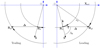 |
Fig. 1 Geometrical configuration of a planet observation by Planck. Left and right frames: trailing and leading observations respectively. The position of the spacecraft is denoted by RS, the position of the planet by Rpl. The Sun is indicated with the symbol ⊙. Both the spacecraft and the planet revolve counter-clockwise around the Sun in circular and coplanar orbits. For a detailed discussion of the symbols, see the text. |
 |
Fig. 2 Time dependence of the angle between Jupiter’s direction and the spin axis of the Planck spacecraft. The darker horizontal bar indicates the angular region of the 11 LFI beam axes, while the lighter bar is enlarged by ± 5°. Saturn, Uranus, and Neptune show a similar pattern. The labels SS1…SS8 denote Planck sky surveys, as defined in Planck Collaboration V (2016), from which the figure is taken. Tr1…Tr7 denote the transits; letters T and L indicate whether it was a trailing or leading transit, according to Fig. 1. |
2.2 Modelling of planet signals
The power collected by a horn pointing towards some direction  close to a planet is the sum of four components:
 (5)
(5)
where ΔIin,p is the power delivered by the planet, ΔIin,bck the power from the background minus ΔIin,block the radiation coming from the background but blocked by the planet, and ΔI0 the noise from the instrument.
The signal from a generic source with spatial brightness distribution  (flux over solid angle) and SED S(ν) is written as
 (6)
(6)
where τ(ν) is the instrumental bandpass;  is the pattern of beam response at frequency ν for a pointing direction
  in the beam reference frame; and
  is the matrix describing the transformation from the ecliptic reference frame to the beam reference frame4, accounting for the beam pointing direction
  and orientation
  at the time of observation5. We assume that τ(ν) ≤ 1, with total bandwidth Δν = ∫ τ(ν) dν and central frequency νcent = ∫ τ(ν)ν dν∕Δν. In the following, the dependence on
  and
and  is omitted. If
  is the versor of the Z-axis of the beam reference frame, aligned with the beam optical axis
  , then
  is the peak value of the beam. The quantity
 (7)
(7)
is the beam solid angle at frequency ν. If beam normalization is assumed to have  then
then  . In this paper, we follow the usual convention to map the main beam over a Cartesian (u, v) system drawn on a plane normal to
  in the beam reference frame, so that pointing
  corresponds to the following (u, v) coordinates:
 (8)
(8)
We indicate band-integrated quantities using the apex ⋅(ba), such as  , S(ba), and so on. Therefore, for a generic source it holds that

2.3 Estimation of planet signals
We now tackle the problem of connecting the quantities in Eq. (5) to the SEDs of the planets, background, and blocking radiation. For this purpose, we now detail the model behind each of the terms in that equation. Using the conventions presented in the previous paragraphs, the integrated power for planet, background and blocking terms are written as

where  is the band averaged black-body brightness; it is assumed that the planet is an extended source with solid angle
  and that most of the blocked radiation is the CMB with SED Bν(Tcmb, ν), so that
 (15)
(15)
In the equations above, we used the following definition:
 (16)
(16)
which denotes the band-averaged beam response for a planet located within the main beam at epoch t. This stems from the fact that  is the position of the planet with respect to the beam reference frame, where
  is the direction in which the planet is seen at time t in the ecliptical reference frame centred on the spacecraft. The difference between
  and
and  is in the SED used to compute the band-averaged integral. Usually,
  and
and  are averaged accounting for the background SED, but in the following sections we do not account for this detail.
2.4 Converting signals to antenna temperatures
We now provide the equations we used to connect SEDs to antenna temperatures, which are the quantities that are actually measured by the instrument. Calibration of radiometers maps the measured input power ΔIin onto a scale of antenna temperature variations based on the cosmological dipole, whose antenna temperature ΔTdip depends on the pointing direction  (Planck Collaboration V 2014, 2016). If we assume that the gain is linear, applying Eq. (6) to the cosmological dipole
 (17)
(17)
where ΔTdip is the temperature fluctuation of the cosmological dipole, convolved with the appropriate band-averaged beam pattern

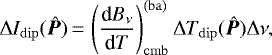
Therefore, the planet signal is mapped onto an equivalent variation of thermodynamic temperature through ΔTant,p∕ΔTdip = ΔIin,p∕ΔIdip. Assuming that the planet is aligned with the centre of the beam, the variation of antenna temperature caused by the presence of the planet is given by
 (21)
(21)
During a transit, the planet motion within the beam causes a time modulation of the antenna temperature  . Therefore, the planet antenna temperature
  for each transit and radiometer can be estimated through the minimization of the quantity
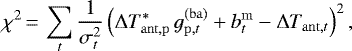 (22)
(22)
where σt is the confusion noise for the sample at time t,  the background model discussed in Appendix A.2, and
  the beam model described in Appendices A.3 and A.4. A rigorous treatment would also include a term to account for the blocked radiation
 (23)
(23)
by the addition of a term  in Eq. (22), as shown in Appendix A.9. This would lead to an estimate for
  that is already corrected for the blocking factor. However, since blocking is a minor effect, it is customary to correct it later. We chose to follow this approach, and therefore in this work
  does not include correction for blocking. This convention introduces a small systematic effect, since
  . Table 1 summarizes all the radiometer-dependent quantities that are relevant for photometric analysis, which we presented in this section, together with other parameters that are discussed later.
3 Data analysis
In this section, we describe the data analysis procedures used to implement the equations presented in Sect. 2. The results of our analysis are discussed in Sect. 4. Since it is not possible to list the full set of measurements per planet, transit, and radiometer in this paper, we present only summary plots showing data at various data reduction steps. The technical details of our data analysis pipeline are explained in Appendix A.
3.1 Characteristics of the input data
In our analysis, we used the Planck 2018 data release, whose timelines were calibrated using the procedure described in Planck Collaboration II (2020). We do not detail the procedure used to produce these data, it is sufficient to recall that in the Planck/LFI 2018 data processing pipeline (i) The timelines are cleaned of the dipole signal; (ii) the Galactic pick-up through beam sidelobes has been removed; (iii) ADC non-linearities are corrected, (iv) the pointing is corrected for a number of systematics6. Each sample in the LFI timelines consists of the following fields: (i) the UTC time of acquisition; (ii) the antenna temperature Tant, calibrated in Kcmb; (iii) the apparent pointing direction  (direction of the beam axis) in the J2000 reference frame; (iv) the beam orientation in the sky; (v) the quality flags; (vi) the absolute address of the sample within the global mission timeline. The pointing directions and beam orientations can be used to compute the Ubeam,ecl,t matrix for the sample.
To produce sky maps from timelines, the Planck/LFI pipeline needs to reduce the level of noise in the timelines. Planck/LFI timelines suffer from the presence of correlated noise, whose spectral shape can be approximated by the function
![\begin{equation*}P(f)\,{=}\,\left[1 + \left(\frac{f_k}f\right)^{\alpha}\right] \frac{\sigma^2}{f_s}, \end{equation*}](/articles/aa/full_html/2021/03/aa37788-20/aa37788-20-eq59.png) (24)
(24)
where f is the frequency, fs is the sampling frequency of the detector, σ is the level of white noise in the data, and fk is the so-called knee frequency of the 1∕f noise; in the case of the Planck/LFI receivers, fk ≈ 20−60 mHz (Mennella et al. 2010). The presence of 1∕f noise invalidates many assumptions used in common data analysis tasks, and several works have dealt with the problem of removing it from time streams. One of the most simple yet effective solutions is the destriping algorithm, which is able to determine the time dependence of 1∕f noise through an approximation of the noise time stream with a number of simple basis functions (Maino et al. 2002; Keihänen et al. 2004). Each basis function is constrained by the requirement that each pass on the same pixel should yield the same measurement if the noise part in Eq. (24) were negligible. In its simplest incarnation, a destriper uses constant-valued basis functions: in this case, each function is called a baseline, and its duration in time must be smaller than 1∕fk in order for the destriper to be effective.
Madam (Keihänen et al. 2004), the map-maker implemented in the Planck/LFI pipeline, uses a destriping technique to produce frequency maps that are cleaned from correlated noise and a set of baselines that approximate the correlated noise in the timeline. However, we were not able to use this information to clean the timelines in our analysis. One of the fundamental assumptionsof the destriping algorithm is that the signal measured on the sky must be constant in time. Therefore, the LFI pipeline masks all those samples acquired while a moving object was within the main beam, and these samples are not considered in the application of the destriping algorithm. We must add that the destriping technique is able to find a reliable solution if there are enough crossings of the same point in the sky among different scan circles. We attempted to use destriping on each planet transit within the main beam of each radiometer: as one transit lasts only a few hours, planets can be considered as fixed point sources. However, the quality of the solution was poor because the number of rings was not sufficient to fully constrain the solution. A comparison of the estimates for  obtained with and without the application of destriping show differences within the random errors due to white noise. For this reason, we decided not to use destriping in our pipeline.
Photometric parameters for Planck/LFI radiometers and band averaged beams.
3.2 Overview of the analysis procedure
To estimate the antenna temperature  for the sources considered in this work, we minimized the value of χ2 shown in Eq. (22). We only considered those samples that were acquired when the point source fell within a circular region of interest (ROI) centred on the main axis of the beam (details are provided in Appendix A.1), whose radius is always 5°, regardless of the radiometer, transit, or planet. An example of the ROI is shown in Fig. 3. As in Planck Collaboration V (2014) and Planck Collaboration V (2016), the background was estimated by splitting the ROI in two concentric circles: the “planet ROI” and the “background ROI” (see Fig. 3 and Appendix A.1). However, unlike Planck Collaboration V (2014) and Planck Collaboration V (2016), we did not consider the background as a constant but we allowed for spatial variations of the background, as described in Appendix A.2. This permits us to remove weak background sources and to mask bright sources, as we show in Fig. 3. We modelled the beam
  using a band-averaged map of the main beam, described in Appendix A.3. We accounted for the apparent motion of the planet and the background within the beam during the acquisition of a sample using the so-called smearing algorithm, which is described in Appendix A.4.
Figure 4 shows the regression of  for Jupiter, Saturn, Uranus, and Neptune for the first transit and for the three radiometers LFI27-0, LFI24-0, and LFI18-0, which are representative of the 30 GHz, 44 GHz, and 70 GHz frequency channels, respectively. Samples are plotted as a function of the radial distance between the planet and the beam centre. The blue and green points represent samples in the planet and background ROIs, while the grey points represent samples not used in the fit; the best-fit model is represented by red points. The dispersion of red points as a function of radial distance is mainly caused by the ellipticity of the beam. This did not occur for WMAP, as the WMAP team used a symmetrized beam (Weiland et al. 2011; Bennett et al. 2013). We note that there is an apparent increase in dispersion for large radius. Thisis not due to an actual increase in the variance of the samples, but to the fact that at larger distances the population of samples increases in size, thus widening the spanning of the plotted points. The LFI data for Jupiter and Saturn show a S/N that is high enough to be seen in raw data. The same does not hold for Uranus and Neptune.
Figure 5 shows the distribution of the residuals of the fit, radially averaged in constant-width bins; the bars denote the RMS of the residuals in each bin. In most cases, the radial pattern of the residuals is nearly flat, apart from Jupiter 24 and 27, which show a systematic error with a peak-to-peak amplitude ≲ 10−3 Kcmb (to be compared with a temperature of ≈0.3 Kcmb). We chose to neglect this residual, as at this stage it is not easy to understand whether this effect is due to uncertainties in the beam modelor bandpass or other perturbations. Moreover, the definition of a new beam model for Planck/LFI is outside the purpose of this paper.
Figure 6 provides a summary of our measures for  for the whole set of planets, transits, and radiometers. For Jupiter and Saturn the dispersion of
  is only partially affected by random noise, which introduces a RMS scatter in
  of at most a few 10−4 Kcmb. When converted into a relative error per planet, transit, and radiometer, the order of magnitude for Jupiter is 10−3, for Saturn 10−2, about 5 × 10⁻¹ for Uranus, and up to 1 for Neptune. The range of errors for our estimates are provided in Table 2.
Because of the small S/N, in some cases the signal for Uranus and Neptune is consistent with zero. This occurs when the confusion noise from the instrument and the background are larger than the signal induced by the planet. Whenever this happened, we removed the affected data from our analysis.
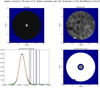 |
Fig. 3 Example of a map in the (u, v) reference frame for Jupiter. This image shows the first transit as seen by radiometer 27–0 (30 GHz). Top left: map of Tant in Kcmb ranging from − 4 × 10⁻⁴ Kcmb to 0.4 Kcmb. Top right: map of the background model, expressed as Tant in Kcmb ranging from − 4 × 10⁻⁴ Kcmb to 1 × 10⁻³ Kcmb. Bottom left: histogram of Tant in Kcmb for the background. The green points indicate the samples in the histogram, the red line indicates the best-fit Gaussian distribution,and the threshold for the classification mask is shown by the dashed blue line. Bottom right: classification mask. The grey region shows the planet ROI, the white annulus is the background ROI, and the blue regions denote unused samples. |
Error bars for ΔTant,p.
3.3 Estimation of a fiducial antenna temperature
Figure 6 shows some variability among transits and radiometers for the same planet, with a clear pattern in the variation of  within the same frequency channel and transit. As an example,
  for LFI20/21 is larger than for LFI19/22, which in turn is larger than for LFI18/23. The first reason for these discrepancies is the difference in the value of Ωbeam among various radiometers because this value is largest for the radiometers located far from the centre of the focal plane, and produces the bent pattern of the 70 GHz channel or the jump between horn 24 and horn 25 and 26. Secondly, we must consider changes in the circumstances of the observation among different radiometers and transits, which leads to differences in the Planck–planet distance
  (Eq. (1)), and so in Ωp, producing the relative shift of the measurements between one transit and the other. We considered the change in
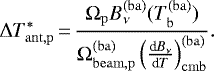
  among different transits and the change occurring while observing the same transit from different horns (refer to Sect. 2.1). Since planets are not spherical and their polar axis are tilted on their orbital planes, varying observing conditions led to different apparent aspect ratios of the shape of the planets. In addition we have to take care of systematics of the beam modelas its numerical efficiency and the beam aperture. We can reduce the antenna temperature to standardized conditions, using the following formula:
 (25)
(25)
where tilted quantities indicate fiducial values. For each channel we take as a fiducial value  , the median of the
  for that channel from Table 1. The actual values we used are 1.006 × 10⁻⁴ sterad (30 GHz), 8.263 × 10⁻⁵ sterad (44 GHz), and 1.607 × 10⁻⁵ sterad (70 GHz). Since the planet solid angle Ωp depends on the observer-to-planet distance,
  (Eq. (1)), the reduction to a fiducial solid angle is equivalent to reduction to a fiducial distance. In Table 3, we list the values we used for planet radii, distances to the observer, and solid angles of the planets. Several conventions and approximations are used in the literature to measure distances and solid angles. As an example, distances to Jupiter can range from 4.04 to 5.2 AU. To ease comparisons, we use the same scale of distances and solid angles as WMAP (Weiland et al. 2011; Bennett et al. 2013). The quantity fasp in Eq. (25) is the aspect correction factor described in Appendix A.5; this accounts for the fact that the aspect ratio of the planet seen by Planck changes in time. The parameter faper is the aperture correction described in Appendix A.6, and it corrects for the loss of signal in the background ROI. The quantity xη is a correction factor for the lack of numerical efficiency of the beam. As detailed in Appendix A.7, the limited accuracy in the numerical computation of the beam induces a systematic in the measured fluxes at the level of ~ 10−3. The precise value of xη cannot be determined precisely, but it is in the range ± fη given in Table 1. For this reason, we did not apply the correction, thus assuming xη = 0, and we included this in the overall uncertainty. We provide more details in Appendices A.7 and A.12. In the Planck Collaboration V (2014) and Planck Collaboration V (2016), a correction factor fSL was introduced to account for sidelobes. In this work, this correction is no longer needed because the GRASP beam model already includes the effect of side lobes; Appendix A.8 provides more details.
Figure 7 shows the derived distribution of the values  (Eq. (25)). The dispersion within the same frequency channel is significantly reduced for the 70 GHz and nearly flattens, and all the 44 GHz radiometers are now consistent. Geometric corrections do not affect the dispersion in 30 GHz channels significantly.
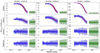 |
Fig. 4 Antenna temperature estimates Tant for Jupiter, Saturn, Uranus, and Neptune (top to bottom) and for three radiometers representative of the 30 GHz (left), 44 GHz (centre), and 70 GHz (right) channels, as a function of the angular distance from the beam centre. The blue bands show the distribution of samples in the planet ROI (dark blue: 1σ region; light blue: peak-to-peak variation). The green bands have the same interpretation, but indicate the background ROI. The grey bands show the data before having been σ-clipped; for the case of Saturn observed by LFI27-0 a point source is present that was removed before the analysis (not present in the green line). The separation between the blue and green lines indicates the presence of the avoidance ROI, not included in our fits. The red line shows the best-fit model, and its width is the root mean square (RMS) of the model due to the ellipticity of the beam. |
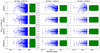 |
Fig. 5 Radial pattern of residuals averaged over the whole set of transits. |
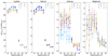 |
Fig. 6 Values of |

Fiducial geometric parameters.
3.4 Reduction of antenna temperatures to brightness temperatures
The result of our estimate is expected to be the brightness of the planet, expressed as a brightness temperature. The brightness for each radiometer and transit can be derived from  with the formula
 (26)
(26)
where  is the correction for the blocked radiation; see also Appendix A.9 and Table 1. We note that the factor
  removes the corresponding correction for standardized observing conditions.
We now turn to the problem of properly defining what we mean with “brightness temperature” Tb, as several definitions are available in the literature. One widely used convention is to define a Rayleigh-Jeans (RJ) brightness temperatureas
 (27)
(27)
where  is the RJ brightness at 1 K estimated at frequency νcent (see also Table 1). This is the convention followed by WMAP (Weiland et al. 2011; Bennett et al. 2013). On the other hand, when data are used to model planetary atmospheres, it is better to define Tb through the inversion of a Planckian curve (de Pater & Dunn 2003; Gibson et al. 2005; de Pater et al. 2016, 2019b; Karim et al. 2018)as follows:
 (28)
(28)
where “c” denotes one of the frequency channels 30, 44, or 70 GHz. In some cases, the following band-averaged formula can be used to define  :
:
 (29)
(29)
where  is the band-averaged SED of a Planckian black body. Its inversion is described in Appendix A.11. Conversion among the different conventions is not difficult, but a detailed model of the instrument bandpass must be taken in account. To simplify the comparison between our results and those from WMAP, and to produce numbers useful for atmospheric modelling, we provide the three quantities Tb,rj, Tb,c, and
  when needed7.
Figure 8 is a summary of the channel-averaged  for each single transit and planet as a function of the quantity DP, the sub-Planck latitude at the epoch of the observation as seen from the planet; it represents the planet aspect angle as seen from Planck. Since we already include the effect of band-averaging in Eq. (26), we do not need any colour-correction factor.
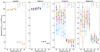 |
Fig. 7 Values of ΔTant,p after reduction to fiducial observing conditions and standardized Ωbeam and Ωp. |
4 Results
In comparing our results with those from WMAP, we must take in account the different value of the dipole amplitude used by Planck and WMAP, as this leads to a mismatch in the absolute calibration level: the Planck team used the value APlanck = 3364 ± 2 μK (Planck Collaboration V 2014, 2016; Planck Collaboration II 2020), while the WMAP team used AWMAP = 3355 ± 8 μK (Hinshaw et al. 2009). Therefore, we scaled the WMAP estimates of Tb,rj by the factor 1.002831. Moreover, WMAP reported Tb,rj rather than Tb,c or  . When needed, we used the WMAP bandpasses to derive Tb,c or
  from Tb,rj, according to the procedure outlined in Appendix A.19. Each of the quantities Tb,rj, Tb,c,
  includes the correction for blocking radiation, as explained in Appendix A.9. The definition of the main symbols is provided in Table 4.
4.1 Jupiter
Table 5 lists the seven transits of Jupiter that have been observed by LFI; the last three transits were not considered in the analysis presented by Planck Collaboration Int. LII (2017). Because of a combination of factors, fewer samples have been acquired in transits 1 and 4. All the transits occur near the Equator, with 0.3° < DP < 3.4° (see Sect. 2.4 for the definition of DP), so that fasp < 3 × 10⁻⁴. The Galactic latitude is always negative, with transit from 1 to 5 between − 62° and − 40°, transit 6 at − 13°, and transit 7 approximately at − 20°. The last twotransits are sufficiently close to the Galactic plane to suffer larger background contamination; this is particularly true at 30 GHz, where Jupiter is weaker and the Galactic background is larger. Figure 8 shows no evident correlations between brightness temperatures and DP. However, transits 6 and 7 at 30 GHz depart significantly from the average. For this reason, we limited our analysis to the first five transits. In total there are 110 measurements (+44 in transits 6 and 7), of which 20 (+8) at 30 GHz, 30 (+12) at 44 GHz, and 60 (+14) at 70 GHz.
Table 6 reports our values for Bp, Tb,rj, Tb,c, and  . We computed these as the weighted averages of the measurements for each frequency channel across the corresponding set of radiometers,still considering five transits. Adding transits 6 and 7 has a minor impact on the 70 GHz channel: Tb,rj = 170.40 ± 0.16 K, Tb,c = 172.08 ± 0.16 K,
  171.07 ± 0.17 K. This is a 0.1 K reduction in temperature, and a marginal improvement on the error bars. Since we consider band-averaged quantities, we used the weighted average of the individual νcent or νcent,eff of each radiometer as the reference frequency. We did not include the effect of the beam numerical efficiency fη (Appendix A.7) in Table 6, so we added an uncertainty of 0.3%; the calibration uncertainty introduces an additional 0.1% to the error budget.
To derive the averaged values in Table 6, we had to consider some subtleties in the analysis; these are described in Appendix A.12. Of course, averaging Bp and Tb,rj is not the same as averaging Tb,c and  , as these are not additive quantities. A more rigorous approach requires us to determine the values of Tb,c and
  that fit the observed Bp; this can be done through the minimization of the function of merit in Eq. (A.13), Appendix A.12. We verified that a simple average agrees with the result of a minimization within the second decimal figure, given the observing conditions of Planck/LFI. However, the numbers we report in Table 6 were derived using the rigorous approach.
Estimating uncertainties is more subtle, as several effects are to be considered. Firstly, there is a large variability in the error bars for Tb,rj, which are denoted as δrndTb,rj: in fact, δrndTb,rj varies from 0.06 to 0.26 K (1σ), These variations can look puzzling, but the transit-to-transit variability in δrnd Tb,rj is highly correlated with the number of samples NP in the planet ROI: the correlation coefficient between  and δrndTb,rj is ≥ 0.96. If we assume that the average of δrndTb,rj across a channel is representative of the uncertainties in the data, we should expect overall errors to be
  ,
,  , and
, and  , for the 30, 44, and 70 GHz channels, respectively. However, this is not what we see in Table 6, as the errors reported are of the order of 0.2 K, which are comparable to the worst δrndTb,rj on a single measure.
Another indication of some possible systematic error in our data is the scatter of Tb,rj among transits, which exceeds what would be expected from a normal distribution with variance  . The standard deviations for Tb,rj are 0.800 K at 30 GHz, 1.072 K at 44 GHz, and 1.439 K at 70 GHz, while peak-to-peak variations are 3.38 K at 30 GHz, 4.13 K at 44 GHz, and6.06 K at 70 GHz. Moreover, the distribution of the residuals is not Gaussian.
Figure 7 shows that the estimates for ΔTant at 70 GHz are distributed around the mean, but they are not completely compatible with random fluctuations. A closer inspection reveals that most of the effect comes from data collected by the radiometers associated with horns 18 and 22. The averaged Tb,rj from horn 18 deviates by − 2.5 K from the average for 70 GHz, while for horn 22 the deviation is + 2. K; for others, the difference is less than 0.5 K, which is compatible with the hypothesis of random noise fluctuations. However, removing these samples does not change the results in the table significantly; as an example, we obtained  K instead of
  K (but the 1σ error decreases from 0.19 to 0.11 K).
Part of the observed variability across radiometers is intrinsic to the source, given the relatively wide bandwidth of our frequency channels, especially at 70 GHz (Planck Collaboration V 2016). This means that introducing some correction to flatten this effect would introduce another kind of distortion in the data. However when computing uncertainties on channel averaged quantities, the adequacy of usual error propagation formula must be assessed. To validate our estimates for uncertainties given by least-square fits, we used a bootstrap technique and a Markov chain Monte Carlo (MCMC). In case of significant discrepancies, we picked the largest error estimate.
Values of Tb,rj, Tb,c, and  in Table 6 are very similar, with differences smaller than 2 K (~ 1%). This happens because the brightness temperature of Jupiter is greater than 140 K: since the radiometers of Planck measure frequencies below 100 GHz the difference between Planck’s law and the RJ approximation is not large. However, the difference exists and explains the fact that
  at 30 GHz and the opposite at 44 and 70 GHz. In fact, below 30 GHz Planck’s law is sufficiently approximated by the RJ law with brightness scaling as ν2; in this case, the band averaged brightness is larger than the RJ brightness computed at the central frequency. Consequently,
  is needed toexplain the same brightness. At higher frequency, the two laws diverge more significantly, and the band-averaged brightness is always lower than the RJ brightness at central frequency; therefore,
  is needed to explain the same brightness. The critical frequency where this swap occurs is mainly determined by the bandwidth: for 30 and 44 GHz radiometers, the critical frequency is in the range 29–37 GHz, while for 70 GHz radiometers is 53–60 GHz. The central frequencies for the 30 GHz channel are just below the critical frequencies, while the opposite happens for 44 and 70 GHz radiometers,thus explaining the observed difference. We provide a more quantitative discussion in Appendix A.14.
In Fig. 9 we plot the estimates for  reported in Table 6 and compare these with a selection of results and models available in the literature. Points are plotted at νcent for each frequency channel. The violin plots at the top give insight into how τ(ν) changes within each frequency channel. The quoted error bars are comparable with the size of the symbols, even including the effect of the ± 0.3% fη correction uncertainty. The black points in the figure represent the WMAP measurements, taken from Weiland et al. (2011) and Bennett et al. (2013), and converted to
  as detailed at the begin of this section and in Appendix A.19. The WMAP results compare well with ours. The plot includes measurements taken from8 Joiner & Steffes (1991), Greve et al. (1994), Gibson et al. (2005), Karim et al. (2018) and de Pater et al. (2019a). The results from Gibson et al. (2005) are measures provided by Klein & Gulkis (1978) (Tab.II in the paper) and reprocessed. According to the conventions used in this paper they are similar to Tb,c.
Apart from WMAP, Fig. 9 compares our estimates with other results found in the literature. The few measurements above 40 GHz are consistent with our estimates; the error bars are however large, and the consistency is therefore of little significance. Below 40 GHz, the situation is much better. In particular, the CARMA measurements in Karim et al. (2018) cover the 27.7–34.7 GHz fairly well. Our estimate at 30 GHz is consistent with CARMA, but we see an excess in  of nearly 2 K. As we explain below, this excess is likely due to the presence of a synchrotron contribution to the Jupiter signal that has been removed in the CARMA data (Karim et al. 2018).
The sparse frequency coverage of measurements in the literature makes it difficult to quantitatively compare our measurements with those of other authors without adopting an interpolation scheme. But microwave emission of Jupiter cannot be reduced to a simple polynomial expression at Planck/LFI frequencies. The emissivity observed outside the atmosphere is the result of the radiative transfer of microwave emission produced by different layers within the atmosphere that radiate towards the observer and are extinguished by the traversed layers (see de Pater & Massie 1985; Gibson et al. 2005). At Planck/LFI frequencies, extinction is dominated by the NH3 absorption. For this reason, it is interesting to compare our data with representative models in the literature, but before discussing the comparison with models, we note that this paper is devoted to the presentation of Planck/LFI data and not to a detailed discussion of models for planetary thermal microwave emission.
We take as a reference the Jupiter radiative-transfer (RT) model described in Karim et al. (2018). The model estimates the full-disc thermal emissivity  of Jupiter for wavelengths between 0.3 and 4 cm and compares well with a number of observations, including CARMA and WMAP seven-year measurements. In the plot,
  is represented by a thick black line. The dashed lines are two further models provided by Karim et al. (2018), which represents an upper and a lower limit for the predicted
  . Our estimates and the model agree very well at 70 GHz, but we overshoot the model at lower frequencies; in particular, at 30 GHz the overshoot is almost 2 K. This happens because at frequencies below 40 GHz the measurement is affected by a small synchrotron emission due to solar high-energy electrons trapped in radiation belts (analogous to Earth’s Van Allen belts) within a few Jupiter radii from the planet (Klein & Gulkis 1978).
For Jupiter, the synchrotron emission is mainly concentrated around the equatorial plane, with two emission lobes clearly seen in Very Large Array maps (de Pater 1981; de Pater & Dunn 2003; Kloosterman et al. 2005), and this emission is polarized at the level of 20–25% (de Pater & Dunn 2003). Gradual changes over time in the total intensity of the emission have been reported by Klein et al. (2001), Dunn et al. (2003) and Kloosterman et al. (2005) at 2.3 and 1.4 GHz. These are mainly connected to secular changes in the density of relativistic electrons in the Jupiter magnetosphere (Dunn et al. 2003; Kloosterman et al. 2005), thereby leading to changes in the synchrotron total intensity but not in its spatial distribution, and to a minor extent to changes in viewing geometry. Abrupt changes in both the intensity and spatial distribution were recorded as a consequence of impacts of minor bodies with Jupiter, as in the case of comet Shoemaker-Levy 9 in 1994 (de Pater et al. 1995; Klein et al. 2001) and of an unidentified object in July 2009 (Santos-Costa et al. 2011), a few months before the first scan of Jupiter from Planck. While WMAP did not attempt any removal of this contribution (Weiland et al. 2011), it is expected to amount to about 1% of the thermal emission of the disc at 28.5 GHz (Karim et al. 2018). Therefore, this effect is comparable or larger than our error bars.
To include the amount of contamination from synchrotron emission, we follow the formalism in de Pater & Dunn (2003), Weiland et al. (2011) and Karim et al. (2018). According to this formalism, the synchrotron emission seen by an observer at Earth has a ν−0.4 spectral dependence, and at the reference frequency of 28.5 GHz the expected synchrotron flux is Fsync = 1.5 ± 0.5 Jy (de Pater & Dunn 2003; Karim et al. 2018), assuming Jupiter as seen at Δ = 4.04 AU corresponding to an  . The total brightness is the sum of the thermal and synchrotron components as follows:
 (30)
(30)
where  is derived from the RT model.
The addition of the 1.5 Jy synchrotron emission explains the 30 GHz overshoot. To better constrain our data, we left Fsync as a free parameter and fitted it against the 30 and 44 GHz data taken separately and then together. We fitted band averaged brightness from models against the individual B(ba) for each transit and radiometer. This is obtained by replacing BRT+sync(ν) and the ν−0.4 dependence with the corresponding band-averaged quantities in Eq. (30) as follows:

where  is tabulated for each radiometer in Table 1.
To analyse the effect of the uncertainty on the beam numerical efficiency correction fη, we scaled B(ba) by (1 ± fη) obtaining an upper and a lower limit for Fsync. Similarly we accounted for the uncertainty in the  model by replacing the best-fit model in Fig. 9 with the upper or the lower limits models represented by the dashed lines. The best-fit Fsync and its uncertainties were derived with the fitting methods already discussed above; we used a bootstrapping algorithm to validate these uncertainties.
Results are shown in the bottom part of Table 7 for the 30 and 40 GHz alone and then taken together. The top part of the table lists weighted averages of  taken across the data sets, and of
  computed for the final model and its lower and upper limits. At 30 GHz the best fit is for Fsync = 1.50 ± 0.15 Jy, to be compared with the expected Fsync = 1.5 ± 0.5 Jy. The uncertainty introduced by the unknown numerical beam efficiency increases the width of the confidence region to 1.15 Jy < Fsync < 1.84 Jy. If we use the best-fit model of Karim et al. (2018) with the lower or the upper limit, we get Fsync = 2.83 Jy and Fsync = 0.47 Jy, respectively. The 44 GHz suggests an higher value, Fsync = 2.53 Jy, but the uncertainty is larger; moreover, the upper model would not require any synchrotron component. Combining 30 and 44 GHz gives nearly identical results to the 30 GHz alone. The thermal model plus Fsync = 1.5 Jy computed from Eq. (30) is represented by the red line in Fig. 9. The grey band represents the difference between upper and lower limit models. The effect of the uncertainty in the fη correction is comparable to the width of the red dots, and it is not displayed. The inclusion of transits 6 and 7 affects mainly the 30 GHz; in this case, the best fit leads to Fsync = 1.75 ± 0.12.
The presence of some synchrotron could potentially introduce a source of variability for the Jupiter disc averaged brightness. However, apart from the case of transits 6 and 7 at 30 GHz, we found no other significant correlation with time or with the geometry of observation in our transit-averaged data. Therefore, we may conclude that during our observations Jupiter behaved as a stable microwave source within ~ 10−3 over three years, in agreement with Weiland et al. (2011).
Before going further, we want to note that Planck Collaboration V (2016) reports slightly different results for Jupiter. This is caused by a number of small differences in data processing; the most important is the evaluation of faper, as explained in Appendix A.6. In addition, Planck Collaboration V (2016) compared Tb,c (Eq. (28)) with  (including blocking radiation), which have relative differences of −5 × 10⁻⁴ to −3 × 10⁻³, equivalent to −0.07 to −0.44 K at 30 GHz, 2 × 10⁻³ to −3 × 10⁻³ equivalent to 0.3 K at 44 GHz, and 6 × 10⁻⁶ to −5 × 10⁻³ equivalent to 0.1−0.8 K at 70 GHz.
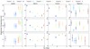 |
Fig. 8 Values of channel-averaged |

Observing conditions of Jupiter per transit.
Channel-averaged results for Jupiter, excluding transits 6 and 7.
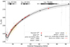 |
Fig. 9 Comparison of Jupiter measurements made in this paper (red circles) with WMAP (black points, taken from Weiland et al. (2011); Bennett et al. (2013) and converted to
|


Derivation of Fsync from the overshooting of 30 GHz and 44 GHz.
Observing conditions of Saturn per transit.
Channel-averaged Tb,rj and Bp for Saturn, for each transit.
4.2 Saturn
Saturn was observed in eight transits, all of which occurred with DP > 0°; Saturn did not cross the Galactic plane in any case. The observing circumstances for Saturn are listed in Table 8; 0.4 we note the higher sampling density in transits 2, 4, and 5. Because of changes in the scanning strategy of the Planck spacecraft, only horns 24, 27, and 28 observed Saturn during transit 5. Transits from 1 to 4 happened simultaneously with Planck/HFI(Planck Collaboration Int. LII 2017), while transits from 5 to 8 were observed by Planck/LFI alone. Transits 1 and 2 occurred near the last two WMAP seasons (Bennett et al. 2013). In total, there are 326 measurements: 96 made by 70 GHz channels, 50by 44 GHz channels, and 36 by 30 GHz channels.
Table 9 lists the weighted average of Tb,rj and Bp for each transit and channel. Errors in the averaged Tb,rj and Bp are derived using usual error propagation and are cross-checked both with bootstrap and Monte Carlo simulations. The 44 GHz channel is divided in two sub-channels: 44(24) refers to horn 24, and 44(25–26) refers to the average of horns 25 and 26. This split accounts for the fact that the transits in horn 24 and in the pair 25–26 occurs about five to nine days apart. The correction for blocking in both Tb,rj and Bp is already introduced. The correction for the beam numerical efficiency fη is not, this adds an uncertainty in Tb,rj or Bp of ± 0.30 K (or ± 7.45 MJy sr−1) for the 30 GHz channel, ± 0.13 K (or ± 7.81 MJy sr−1) for the 44(24) GHz sub-channel, ± 0.22 K (or ± 12.12 MJy sr−1) for the 44(25-26) GHz sub-channel, ± 0.44 K (or ± 66.89 MJy sr−1) for the 70 GHz channel independent from the transit down to the second decimal figure. The difference in magnitude for the effect in the 44(24) GHz and 44(25-26) GHz is connected to the location of the feed horns in the focal plane. Horn 24 was between the 30 GHz, while horns 25 and 26 where on the opposite site of the focal plane with respect to horn 24.
The aspect-angle correction we applied to other planets is unreliable in the case of Saturn, because of the presence of the rings. They emit microwave radiation and partially extinguish the microwave emission radiated from the regions of Saturn’s disc along lines of sight intersecting both the ring and the disc. On the other hand, they scatter but do not block background radiation (Weiland et al. 2011).
Following the approach in Weiland et al. (2011), Bennett et al. (2013) and Planck Collaboration Int. LII (2017), we used an empiricalmodel to separate the disc and the ring contribution as follows:
 (33)
(33)
where Tb,rj are the RJ brightness temperatures quoted in Table 9 for each frequency channel and transit, Td and Tr are RJ temperatures for the disc and the rings (free parameters of the model),  is the equatorial solid angle of the disc, Ωc,r is the solid angle of the fraction of the disc that is hidden by the rings, Ωuc is the solid angle of the unimpeded disc, Ωuh,r is the solid angle of the part of ring r that is not obscured by the disc, and B = DP is the ring opening angle. All the quantities are calculated at the epoch of the given transit. Rings are numbered starting from the outermost (ring A is r = 1) to the innermost (inner C is r = 7). The radii of the rings and their optical depths τr are fixed parameters of the model and are taken from Table 10 of Weiland et al. (2011), which follows Dunn et al. (2002). The possibility of considering all the τr as free parameters was discussed in Weiland et al. (2011), Bennett et al. (2013), and Planck Collaboration Int. LII (2017), without conclusive results; because of our error bars, we decided to keep them as fixed parameters.
For each set of observations, we derived Td and Tr through the minimization of the quantity
 (34)
(34)
where t runs over the list of transits, and wD,t and wR,t are abbreviations for the coefficients in front of Td and Tr in Eq. (33). In general, wD,t + wR,t≠1. The weights wD,t and wR,t are weighted averages of coefficients derived for each radiometer in a given channel and are tabulated in Table 9.
Figure 10 shows Tb,rj for each transit and frequency channel as a function of the planet aspect angle DP. Continuous curves show the best-fit model of Saturn brightness temperature, obtained with different data cuts: (1) all the transits, (2) all but 7 and 8, and (3) all but 3, 7, and 8. The reason why we considered transit 3 as peculiar is the occurrence of a massive Saturnian storm during the transit (Janssen et al. 2013). The exclusion of transits 7 and 8 is motivated by the fact that an analysis performed including those transits produces a significantly lower Tr than expected from WMAP and literature measurements. This anomaly is more important at 70 GHz, but it can be traced in the other channels as well. Therefore, at 70 GHz the expectation from WMAP is Tr ≈ 16 KRJ, while Planck/LFI data lead to Tr = 11.6 ± 1.0 KRJ (all transits), Tr = 13.9 ± 1.0 KRJ (no 7 and 8), and Tr = 16.2 ± 0.7 KRJ (no 3, 7, and 8). Moreover, the reduced χ2 for the three cases shows a clear progression:  , 4.1, 0.97. Inspection of Fig. 10 suggests that the reason for this anomaly resides in the fact that Tb,rj for transits 7 and 8 are too low when compared to the other transits. We have no explanation for this result because there were no background sources bright enough to disturb our measurements during those transits, and there were no obvious anomalies in the timelines. We note that the massive Saturnian storm was still visible in 2015 (de Pater et al. 2018); however, without other independentobservations to compare, we decided to tag transits 7 and 8 as anomalous. In the remaining discussion, transits 3, 7, and 8 are not used in the fit.
Table 10 gives the list of fitted Tr, Td for each channel excluding transits 3, 7, and 8. As for the other planets, disc RJ brightness Td are also converted to Td,c which are equivalent to a Tb,c for the other planets, and to  which are equivalent to a
  . The former are derived from Td using
  , where
  and wt,r are the weights per transit and radiometer (t, r) used to derive the Tb,rj in Table 9 and the latter are obtained through a numerical inversion of
  , where
  . As our starting point is Table 9, Td is already corrected for blocking, we verified that adding the blocking correction to Tb,rj has a minor effect on Tr compared tothe errorbars. As usual we estimated errors using error propagation, bootstrap, and Monte Carlo simulations. We find a good agreement between the three methods, but where differences were relevant, we quoted the largest one. The effect of fη is equivalent to add a systematic uncertainty of ± 0.35 K for the 30 GHz channel, ± 0.13 K for the 44(24) GHz sub-channel, ± 0.26 K for the 44(25-26) GHz sub-channel, and ± 0.46 K for the 70 GHz channel at Td, Td,c and
  . For Tr the uncertainty is ± 3.5 × 10⁻³ K for the 30 GHz channel, ± 8.6 × 10⁻² K for the 44(24) GHz sub-channel, ± 2.0 × 10⁻² K for the 44(25-26) GHz sub-channel, ± 4.6 × 10⁻² K for the 70 GHz channel.
Figure 11 compares Tr in Table 10 with results from Weiland et al. (2011), Bennett et al. (2013) and Planck Collaboration Int. LII (2017). Data from literature are presented as grey marks (Janssen & Olsen 1978; Schloerb et al. 1979a,b; Epstein et al. 1980; Dunn et al. 2005). Moreover, we compared our results with the model of Dunn et al. (2005). Our estimates for Planck/LFI compare well with the other available data. In particular, both Planck/LFI and WMAP measurements fit well the result of Janssen & Olsen (1978) near 40 GHz and with Dunn et al. (2005) at 100 GHz and 110 GHz. Also both for the case of Planck/LFI and WMAP Tr matches a power law of the form  , consistent with the model of Dunn et al. (2005). For WMAP A = (1.35 ± 0.12) KRJ and α = 0.58 ± 0.02, while for Planck/LFI A = (1.36 ± 0.55) KRJ and α = 0.58 ± 0.10. It is interesting to note that Planck/HFI data exhibits a less steep power law with A = (3.88 ± 0.92) KRJ and α = 0.311 ± 0.044, thereby predicting a lower Tr at 70 GHz and a higherTr at 30 GHz; the agreement at 44 GHz is much more significant. When taken together, Planck/LFI, WMAP, and Planck/HFIseem to suggest a change in slope around 100 GHz, but the only measure in significant disagreement with Planck/HFIseems to be that from WMAP 90 GHz. The remaining data from literature are not sufficiently accurate to make a decision. This could be an interesting point for a future observing campaign in the 50–150 GHz frequency range.
Figure 12 compares  for Planck/LFI with WMAP (Weiland et al. 2011; Bennett et al. 2013) and Planck/HFI (Planck Collaboration Int. LII 2017). There is a good agreement between the three datasets, even though our data seem to prefer a slightly warmer disc than those of WMAP. Older data taken from literature (Klein et al. 1978; de Pater & Dickel 1991; Greve et al. 1994; Goldin et al. 1997; Dunn et al. 2005)9 are very sparse in frequency coverage and exhibit wider error bars. In the frequency interval 50–150 GHz, measurements from the literature span the range 135–160 K, but most of the measurements are in the lower side of the interval, while measurements from WMAP andPlanck favour the upper side. The reason could be in the absolute calibration of those old observations, as an absolute calibration error of the order of ten percent is often quoted in these works, and observations are not usually calibrated against the same sources. This is the opposite of WMAP and Planck, which share the same calibration.
Most of the models proposed in literature underestimate the combined WMAP and Planck data; some of those models are presented in Fig. 12. In all these models, the atmosphere is assumed to have abundances of NH3, H2O, H2 S, CH4 enhanced with respect to the Sun by a factor of 3, 5, 11 and 5, respectively. The first model presented in the figure (de Pater & Mitchell 1993, labelled “de Pater and Mitchel (1993,A)”) does not include any contribution from cloud absorption, and this model underestimates the observed brightness below 90 GHz; above this frequency, the first model matches our data, but overestimates the majority of the older measurements. The inclusion of clouds with NH3 ice, H2O liquid, and ice, NH4SH ice leads to the model labelled as “de Pater and Mitchel (1993,D)”, which underestimates our measurements. Similar behaviour appears with the models in van der Tak et al. (1999), with abundances of NH3, H2O, H2 S, CH4 enhanced bya factor of 1.9, 4, 11, and 4 with respect to solar values (not shown, for brevity), and in Dunn et al. (2005), which is an improved version of the nominal model in de Pater & Mitchell (1993). Encrenaz & Moreno (2002) proposed two models with two different profiles for the extinction of the NH 1.28 cm line: BRJS (Ben-Reuven 1966; Joiner & Steffes 1991) and VVW2, a Van Vleck-Weisskopf profile (de Pater & Massie 1985; Lellouch & Destombes 1985; Moreno 1998). The authors favour VVW2, since it fits the data in literature better, with the caveat that its model line profile heavily underestimates Planck and WMAP data, while the BRJS fits them much better. We note that neither de Pater & Mitchell (1993) nor Dunn et al. (2005) include the PH3 absorption band at 263 GHz, which is instead present in the last two models.
In Planck Collaboration Int. LII (2017), a model named ‘ESA2 model’ was used to compare Planck/HFI results with WMAP and earlier Planck/LFI results. The predicted brightness temperature is very similar to that predicted by the model in Encrenaz & Moreno (2002), with VVW2 profile. The work also provides uncertainty limits; in particular, the upper limit is very similar to the Encrenaz & Moreno model with BRJS profile; this upper limit fits both WMAP and Planck data. Unfortunately no references or details are given about this model, and for this reason it is not presented in this work.
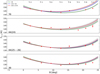 |
Fig. 10 Saturn Tb,rj for 70 GHz frequency channel (first frame from top), 44 GHz frequency channel (second and third frames), and 30 GHz frequency channel (fourth frame) as a function of DP. Labels Tr1, Tr2, …, Tr8 denotes the transit from which each observation originates. Continuous curves refers to the best-fit models of Tb with various selections of data: all transits, transits 7 and 8 excluded, and transits 3, 7, and 8 excluded. The grey bands are 1σ uncertainties in the models. |
Channel-averaged Tr, Td, Td,c and  for Saturn from transits 1, 2, 4, 5, and 6.
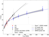 |
Fig. 11 Spectral energy distribution of Saturn rings from Planck/LFI (red), Planck/HFI (blue), and WMAP (black). Data from previous literature outside WMAP and Planck are shown in light grey (references in the text). |
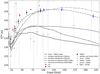 |
Fig. 12 Spectral energy distribution of Saturn disc from Planck/LFI (red), Planck/HFI (blue) and WMAP (black). The model labelled dePater and Mitchel (1993,A) does not include clouds, while dePater and Mitchel (1993,D) includes clouds. For other details about the other models, see the text. |
Observing conditions of Uranus per transit.
Observing conditions of Neptune per transit.
4.3 Uranus and Neptune
Tables 11 and 12 describe the observing conditions for Uranus and Neptune. There are eight transits in which both planets are observed; all the cases transits occurred far from the Galactic plane. For both Uranus and Neptune, the signal is very weak, especially at 30 and 44 GHz, and they are therefore difficult to detect. For Uranus,  is in the range 6 × 10⁻⁵−5 × 10⁻⁴ Kcmb at 30 GHz, 3 × 10⁻⁴−9 × 10⁻⁴ Kcmb at 44 GHz, and 7 × 10⁻⁴−3 × 10⁻³ Kcmb at 70 GHz, While for Neptune
  is in the range 2 × 10⁻⁵−3 × 10⁻⁴ Kcmb at 30 GHz, 4 × 10⁻⁵−5 × 10⁻⁴ Kcmb at 44 GHz, and 6 × 10⁻⁵− 1.3 × 10⁻³ Kcmb at 70 GHz. In some cases, the result of the fit is
  , which means that the planet is not detected: for Uranus, this occurs in transits 2 and 3 for horns 25 and 26, and in transit 3 for horns 24, 27, and 28; for Neptune, this occurs in transit 3 for radiometers 25M and 28M. We decided not to include these data in our analysis.
Figure 8 shows that the scatter in the channel averages for each transit are consistent with the error bars, except for  at 30 GHz in transit 2, and at 70 GHz in transit 3. We removed these two data points before computing the channel averaged results presented in Table 13 (Uranus) and in Table 14 (Neptune). It is known that Uranus has a significant time variability in microwave over a timescale of decades, mainly connected to the change in the DP of the observation (Klein & Hofstadter 2006; Kramer et al. 2008). A relative variation of 0.5%∕year or 0.1% at 90 GHz for one degree of variation of DP was reported by Kramer et al. (2008). Assuming that the same numbers are valid at 70 GHz and a time span between our observations of about 3.6 yr, corresponding to a span of about 20.4° in DP, we expect to detect a change of the order of 2–2.6 %. As shown in Fig. 8, the scatter in our data is larger than this effect; therefore, we decided not to consider it.
Figure 13 compares Planck/LFI Uranus and Neptune  measurements with Planck/HFI measurements at 100 and 143 GHz from Planck Collaboration Int. LII (2017), and WMAP seven-year measurements converted to
 . In addition we show a selection of measurements published in the past literature. The data for Uranus are taken from Gulkis et al. (1978); de Pater & Richmond (1989), Muhleman & Berge (1991), Greve et al. (1994) and de Pater (2018)10; for Kramer et al. (2008); we only show the average of the data. For Neptune data are taken from Cunningham et al. (1981), de Pater & Richmond (1989), de Pater et al. (1991, 2014), Muhleman & Berge (1991), Griffin & Orton (1993), Greve et al. (1994), and Tollefson et al. (2019). Our measurements for both Uranus and Neptune are in general agreement with WMAP, Planck/HFI, and the past literature.
In contrast to Jupiter and Saturn, where the 1.3 cm NH3 inversion line and PH3 transitions significantly affect the spectrum, it has been observed that Uranus and Neptune spectra in the 20–150 GHz smoothly decrease with frequency (de Pater et al. 1991; Encrenaz & Moreno 2002). A simple law can be used to transfer observations from one frequency to the other, similar to the fourth-order polynomial in log10ν provided by Griffin & Orton (1993); in the range of frequencies of interest for this work, this can be reduced to the simpler form
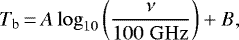 (35)
(35)
with A and B free parameters. For Uranus A = −74.5 ± 31.6 K, B = 118.9 ± 0.9, K, and for Neptune A = −72.3 ± 9.9 K, B = 117.8 ± 0.2 K. The corresponding fit is shown as a grey band in the figures. For Uranus, the discrepancy between the 70 GHz datum and WMAP is ~ 2 K, a bit more than 1%. On the contrary, for Neptune the WMAP V and W bands overestimate both our number at 70 GHz and the Planck/HFI estimate at 100 GHz.
At odds with the expected smooth Tb variation with frequency, the WMAP team noted that Tb in their Ka, K and Q bands (Weiland et al. 2011); the significance of this drop is reinforced by comparison with other observations in the literature. Our results does not disconfirm this finding, as our measure at 44 GHz agree with WMAP Q band, while the 30 GHz datum is between the WMAP K and Ka bands. The combination of all of the observations suggests the presence of a drop in the thermal emission of Uranus, which is centred at about 30 GHz, of about 4–5 GHz and a depth of 20–50 K. However, the uncertainty in the magnitude of the drop is very large; data in literature have wide error bars and use different calibrations. Therefore, we think that more data are needed to validate the existence of this spectral feature.
Models of the microwave emission of Uranus and Neptune are available in Griffin & Orton (1993), Kramer et al. (2008), Griffin et al. (2013) and Bendo et al. (2013). In this work, we consider the models in de Pater (2018) for Uranus and in de Pater et al. (2014) and Tollefson et al. (2019) for Neptune, together with the ESA models used for the calibration of Herschel; the latter has a quoted 5% uncertainty (Moreno 1998; Teyssier & Marston 2017)11. They are included in our figure because they are important for the inter-calibration between Herschel and Planck (Bertincourt et al. 2016; Müller et al. 2016; Planck Collaboration Int. LII 2017).
The model of de Pater (2018) for Uranus assumes abundances of H2O, H2 S, CH4 enhanced of a factor 10 with respect to solar abundances of O, S, and C. Ammonia is kept at solar N abundance and is captured in NH4SH clouds; therefore, it is depleted above the corresponding atmospheric layer. According to this model, at our frequencies opacity is mainly due to H2 S absorption and collisionally-induced absorptions from H2. The figure shows that the model essentially matches our scaling law and only slightly underestimates our 44 and 70 GHz data; it does not predict any drop around 30 GHz.
The ESA2 model for Uranus is an updated version of the model in Moreno (1998) used for the calibration of Herschel. This model was used to validate Planck/HFI data and for comparison with WMAP (Planck Collaboration Int. LII 2017). Our 70 GHz measure is in close agreement with this model, and even the 30 GHz datum agrees with this model. It is interesting to note that the model predicts a decrease of signal around 30 GHz, but it fails to follow the pattern of the spectrum below 45 GHz. Unfortunately, few details are provided for this model, so it is not possible to push the analysis further. After the release of the ESA2 model, the Herschel collaboration proposed another model of the spectrum of Uranus named ESA4, which includes observations from Spitzer (Orton et al. 2014)and extends down to 60 GHz. It is evident that the model significantly overestimates the brightness below 100 GHz.
For Neptune, we considered the model in de Pater et al. (2014). The model featured abundances of H2 S, H2O, and CH4 enhanced by a factor of 30 with respect to solar abundances of S, O, and C, and a wet lapse rate. The model matches our scaling law but underestimated Tb of about 10%. We included in our analysis the model inTollefson et al. (2019)12. It features an abundance of H2S, CH4, and H2O that is 30 times the proto-solar abundance. The model fits the data for Planck/LFI 70 GHz and Planck/HFI 100 GHz and 144 GHz very well, but it underestimates the measurements at 30 and 44 GHz. The ESA2 and ESA5 models are also shown in the figure as blue and orange lines, respectively. ESA5 was used to validate the Planck/HFI data, but it has been not used for the final calibration of Herschel 13. As already noted in Planck Collaboration Int. LII (2017), the model slightly overestimated the brightness temperature in the range 70–200 GHz and underestimated our 30 and 44 GHz data. It is interesting to note the good agreement between ESA2 and our measurement at 70 GHz. For Neptune, both ESA2 and ESA5 models marginally fit our results above 70 GHz, and ESA5 looks slightly better than ESA2.
Channel-averaged results for Uranus.
Channel-averaged results for Neptune.
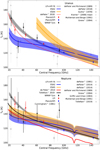 |
Fig. 13
|

5 Conclusions
We analysed the data in the Planck 2018 public data release to characterize the emission of the planets Jupiter, Saturn, Uranus, and Neptune in the frequency range 30–70 GHz, using all the data acquired by the LFI instrument during its four-year lifetime (August 2009–October 2013). In each transit, a planet was observed by Planck/LFI for a few hours rather than days or weeks as in the case of WMAP. Within each transit, the cumulative integration time was about few seconds per planet, transit, and radiometer. The LFI observed Jupiter seven times and the other planets eight times. In the past, just part of those transits were fully analysed in a self-consistent manner. On the contrary, we treated all the observations in a fully homogeneous manner. Moreover, we used our improved knowledge of the beam and bandpasses to refine our earlier analysis.
In the case of Jupiter and Saturn, the sensitivity of Planck/LFI allowed us to reduce the impact of instrumental white noise to a small amount, and the dispersion of our measurements within each frequency channel after geometrical corrections shows a residual variability that is larger than the noise. Calibration uncertainties on individual radiometers could be a source of such variability: in particular, we cannot exclude that part of the radiometer-by-radiometer variability we observed in our sample of Jupiter’s observations could be connected to uncertainties in the model of the bandpass of each radiometer. This could introduce small differences between the calculated radiometers central frequencies, bandwidths, or higher order bandpass moments and the real ones. In principle, by comparing measures of a bright source, such as Jupiter, with a well-calibrated model or set of measures from another instrument, it would be possible to derive a correction for this effect. But if blindly applied, this method forces every other possible residual systematic in this correction. For this reason and because of a lack of a sufficiently accurate model of the emissivity of Jupiter, including non-thermal emission, we did not attempt to derive this kind of correction in this work. We guess that improved calibration methods, such as those described in BeyondPlanck Collaboration (2020), will improve this result.
Despite the difference in the time span of observations, our results are directly comparable to WMAP observations (Weiland et al. 2011; Bennett et al. 2013), which were obtained in a similar range of frequencies. In particular, we confirm the good agreement between the Planck/LFI and WMAP estimates of the SED of Jupiter. Our results improve the frequency coverage in the range 20–90 GHz. A comparison with existing models below 70 GHz allowed us to estimate Jupiter’s synchrotron contribution in the 30 GHz channel in the range 0.9–2.4 Jy. As Planck/LFI and Planck/HFI cover separate ranges of frequencies, to compare these values we had to rely on far-infrared emissivity models for giant planets. The result of our comparison shows a good agreement between the measurements of the two instruments.
Our estimates for Saturn’s disc SED agree with WMAP at 30 GHz, but our results favour a slightly warmer disc at 44 and 70 GHz. With the present knowledge of the instrument it is not possible to assess whether the difference is due to some systematic in either Planck/LFI or WMAP, or if it is connected to the fact that WMAP observations were centred at negative planetocentric latitudes, while Planck/LFI observations were centred at positive latitudes. Given the large error bars of older measurements in literature, we can only say that our measures agree with most of the older measurements. We compared our Saturn’s measurements with known models published in the literature. All but two significantly underestimated the SED in the frequency range considered here. About rings, we may note the excellent agreement of Planck/LFI with both WMAP and existing estimates for frequencies below 100 GHz. Data below 100 GHz show some discrepancy with Planck/HFI, but the existing data does not allow us to assess the significance of this mismatch.
Measures for Uranus and Neptune have very low S/N. For some transit and/or radiometer, confusion noise prevented a proper detection: consequently, error bars are larger than for Jupiter and Saturn, although they agree with those in literature. In particular, our results are in agreement with WMAP and Planck/HFI at 100 and 143 GHz. We compared a selection of existing models for the microwave emissivity of Uranus and Neptune with our data plus WMAP and Planck/LFI. These comparisons show a good agreement in the 100–143 GHz range, but significant discrepancies below 100 GHz. In particular, the Uranus model presented in de Pater (2018) and the Neptune model found in Tollefson et al. (2019) show a better agreement with our data. For observers willing to use these planets as calibrators, we advise that a simple power law is very good at modelling the dependence on Tb for Uranus and Neptune in the frequency range 20–143 GHz within the current error bars.
In earlier generations of CMB experiments, giant planets have been considered good beam calibrators and have been used as calibration sources between different experiments, thanks to their high S/N (Weiland et al. 2011; Bennett et al. 2013; Planck Collaboration V 2014, 2016). Planetary observations will likely maintain the same importance in future missions, such as the planned LiteBIRD mission (Hazumi et al. 2019). The increased demand for accurate and sensitive CMB measurements will necessarily require more accurate models for the analysis of planetary emission in the microwave range. Outer planets, in particular Jupiter and Saturn, have complex spectra and no simple scaling law will work, especially when combining data from detectors with different bandpasses. In this case, people should use reliable models of planetary emissivities (including both thermal and non-thermal components); however, current models have uncertainties that are larger than the measurement errors. An observing campaign with ground-based instruments, coupled with progresses in modelling, could solve this problem.
Acknowledgements
This work is based on the 2018 Release of Planck/LFI data. The writers acknowledges the support of: Planck Collaboration, ESA, ASI, CNR, Università di Milano and INAF (Italy); CNES and CNRS/INSU-IN2P3-INP (France); NASA and DoE (USA); STFC and UKSA (UK); CSIC, MINECO, JA, and RES (Spain); Tekes, AoF, and CSC (Finland); DLR and MPG (Germany); CSA (Canada); DTU Space (Denmark); SER/SSO (Switzerland); RCN (Norway); SFI (Ireland); FCT/MCTES (Portugal); and ERC and PRACE (EU). A description of the Planck Collaboration and a list of its members, indicating which technical or scientific activities they have been involved in, can be found at http://www.cosmos.esa.int/web/planck/. This work have been partially supported by INAF/Trieste Astronomical Observatory through “Ricerca di Base 2019” F.U. 1.05.01.01. M.M. acknowledges Maria Teresa Capria for useful suggestions about models of planetary atmospheres. The authors acknowledge the staff of the Library of the INAF/Trieste Astronomical Observatory: Laura Abrami and Chiara Doz, for their kind help in recovering the needed bibliography during the lockdown imposed in Italy by the COVID 19 pandemic. The authors thank the two anonymous referees for their suggestions, which helped to considerably improve the paper. This research made use of Astropy (http://www.astropy.org), a community-developed core Python package for astronomy (Astropy Collaboration 2013, 2018); EMCEE (https://github.com/dfm/emcee) (Foreman-Mackey et al. 2013) HEALPix (https://healpix.jpl.nasa.gov) (Górski et al. 2005); HEALPy (https://github.com/healpy/healpy) (Zonca et al. 2019); IPython (https://ipython.org) (Pérez & Granger 2007); MatPlotLib (https://matplotlib.org) (Hunter 2007); NumPy (https://numpy.org) (Virtanen et al. 2020); Pandas https://pandas.pydata.org) (McKinney 2010). PyQuarantine (https://www.ict.inaf.it/gitlab/michele.maris/pyquarantine.git) SciPy (https://www.scipy.org) (Virtanen et al. 2020); WebPlotDigitizer (https://automeris.io/WebPlotDigitizer/) (McKinney 2010).
Appendix A Technical aspects of the data analysis procedure
In this appendix, we provide more information about some of the most technical issues we have tackled to produce estimates for brightness temperatures.
Range of variability for ΔTant,p, in mKcmb.
A.1 Selection of samples and ROI
We used the Horizons web service14 to compute the apparent position of the planet for each sample in the time-ordered data acquired by the Planck/LFI radiometers.Using these positions, we selected those samples within the stability period of each pointing period according to the following criteria: they are not flagged as bad and their pointing direction in the sky is within 5° from the planet (the ROI). This radius limits the amount of data to process to a reasonable amount, and enables full coverage of the angular size of the main beam; moreover, it is large enough to estimate the contribution of the background. The 5° angular size separates the intermediate beam region and the far side-lobe region, for which the Planck collaboration provided GRASP beam maps (Planck Collaboration IV 2016).
We divided the 5° radius ROI into three concentric regions: the planet ROI is the ring with radius RROI-I = 1.3 FWHM of the beam used to estimate ΔTant,p; the avoidance ROI is the annulus between RROI-I and RROI-II = 2 FWHM; and finally, the background ROI is everything within RROI-II and RROI. Typical values for RROI-I are about ≈0.7°, ≈ 0.5°, ≈ 0.3° at 30, 44, and 70 GHz respectively,while for RROI-II ≈ 1.1°, ≈ 0.8°, ≈ 0.4°. The number of samples in the planet ROI is in the range 103−104; the number of samples in the background ROI is in the range 105−106. Owing to changes in the scanning strategy during the mission, the density of samples in the ROI largely changed among different transits. As an example, Fig. 3 shows the classification and masking of data in the first transit for radiometer LFI27-0 (30 GHz).
A.2 Background modelling
In the Planck Collaboration V (2014) and Planck Collaboration V (2016), the background was modelled as a constant derived from the median of the background ROI. The constant included contributions from diffused foregrounds, CMB, point sources, and zero-point differences among different radiometers. However, after having masked point sources, the typical RMS of the diffuse background (ΔTant,p) in the background ROI is RMSbackground ≈ 10−4 Kcmb Compared to  for the planets observed by Planck/LFI (Table A.1), it is evident that this fluctuation is equivalent to
  of the Jupiter signal, which is negligible. For weaker planets, background fluctuations are more relevant: for Saturn
  ≈ (0.4 ÷ 3) × 10−2, for Uranus
  ≈ 0.1−0.6, and for Neptune
  ≈ 0.2−1.4. Proper background removal is mandatory for all the planets but Jupiter.
To remove the background, we used the Planck 2018 sky maps to build a timeline bk,t for each transit and each radiometer. These timelines were computed using bilinear interpolation on the sphere at each pointing direction  . As for planets, we considered smearing as well (see Appendix A.4). Since sky maps refer to the central frequency of the channel, the simulated timelines bk,t do not account for differences in bandpasses among different radiometers. To fix this, we introduced a scaling parameter αbck and a zero point zbck in the fit, so that bt = αbckbk,t + zbck. We determined the parameters αbck and zbck for each radiometer by fitting the background model against the samples in the background ROI. Typical αbck varies from 0.5 to 1.3, while zbck varies within ± 0.2 mKcmb.
Figure 3 in the top right frame shows a background map derived from bt. In the bottom left frame, we show the histogram of the background model using green dots, and we overlap a Gaussian distribution with the same mean and RMS (red line). The long tail in the right wing of the distribution is due to the bright source on the bottom left corner of the map. We used a simple σ-clipping, whose threshold is shown as a dashed blue line in the plot, to mask that region (bottom right part of the figure).
A.3 Bandpasses and beam patterns
Equation (22) shows that proper modelling of the beam shape is critical. The results presented in this paper are based on the official band-averaged beam model, computed using GRASP. We derived a band-averaged map of the beam out of a set of gridded monochromatic maps, which were weighted according to the product between theSED of the incoming radiation and the bandpass of the radiometer. For planets, we used a ν2 SED, as it represents the SED of a planet emitting in the RJ regime. To estimate  (Sect. 2.3), we converted the instantaneous position of the planet in the (ut, vt) coordinates using Eq. (8), and we recovered the beam response using bilinear interpolation. There is a strong connection between the reduction of Jupiter observations and the estimation of the beam model because the former requires the latter, but the latter is usually validated through the former. Unfortunately, carrying on the two analysis tasks at the same time is prohibitive, owing to the computational time required by GRASP to estimate beam maps. Therefore, in our analysis we had to assume the correctness of the GRASP beam models produced by the Planck/LFI collaboration.
A.4 Smearing
The signal acquired by Planck/LFI radiometers was integrated over a discrete sampling time, δtsamp, which depended on the frequency of the detector (30, 44, or 70 GHz) and was in the range 0.01–0.03 s. In that time, the planet moved across the beam and causes smearing. Smearing smoothed the signal and it must be properly taken in account in data analysis because it reduced the value of  (about 1.4% at 30 GHz, 1.1% at 44 GHz, and 1.2% at 70 GHz). The amount of smearing was constant, as δtsamp for each radiometer was tuned to allow the beam to move by ≈FWHM∕3.
To model the smearing effect, a common approach is to create a beam map by stacking and averaging a number of repetitions of the simulated GRASP beam map, shifted along the direction of scan by a fixed amount. However, this approach does not account for the fact that the spin rate and the effective boresight angles can change during the mission. Therefore, we used a different strategy to deal with smearing. We over-sampled the modelled beam pattern along the path of the apparent motion of the planet in the beam reference frame and averaged the result.
To compute the planetary smearing for the ith sample taken at time ti, we took a triad of consecutive positions of the planet in the beam reference frame (u, v) at times ti−1, ti and ti+1. Given that the u and v directions are orthogonal, the motion is described by the equations

where l = (t − ti)∕δtsamp, so that l = −1, 0, + 1 for samples i − 1, i, i + 1, respectively. We derived the coefficients Au,i, Bu,i, and Cu,i from the positions ui−1, ui, and ui+1 using least-squares minimization. The result is

and identical expressions can be derived for Av,i, Bv,i, Cv,i replacing u with v. We implemented over-sampling through an evaluation of the beam response over a number of positions Nsmear calculated for  and including the background. Our tests showed that Nsmear = 11 is sufficient. We applied a similar procedure for the background calculation too, as mentioned in Appendix A.2.
A.5 Geometric corrections
Geometric corrections have to be introduced to correct for different conditions of observations, in particular differences in planet-observer distances and planet aspect angles15. The WMAP collaboration reduced all the observations to a fiducial distance before computing Tb (Weiland et al. 2011; Bennett et al. 2013). While this step is not needed to recover Tb, as those effects can be directly accounted in the fit, it is convenient for the discussion to add this step. A geometrical correction factor is defined as
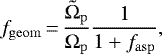 (A.6)
(A.6)
where Ωp is the planet solid angle at the epoch of observation and  is the planet solid angle at an arbitrary fiducial planet-planck distance, in our case the distance of the first transit. Planets are oblate spheroids, so that the solid angle depends on the latitude of the observer as seen from the Planet DP (the sub-Planck point). Consequently, a fiducial Ωp may refer to an observer looking at the pole or at the equator. The difference between the two conventions is 6.9% for Jupiter Tb, 10.9% for Saturn (only the disc), 2.3% for Uranus, and 1.7% for Neptune. We follow the convention in Weiland et al. (2011), Bennett et al. (2013) and Planck Collaboration Int. LII (2017), and we refer to observation at the equator16. In this way,
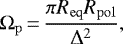 (A.7)
(A.7)
where Δ is the distance of the planet from Planck at the epoch of observation, and Req, Rpol the equatorial and the polar radius of the planet. In our observations, Ωp are in the ranges (2.7−3.1) × 10−8 sterad for Jupiter, (4.8−5.4) × 10−9 sterad for Saturn, (2.2−2.3) × 10−10 sterad for Uranus, and (9.4−9.6) × 10−11 sterad for Neptune.
The term fasp accounts for the fact that the planet is not always seen with the same aspect angle, that is, the same “sub-Planck latitude” DP:
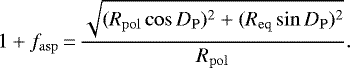 (A.8)
(A.8)
The correction is tiny, as fasp is 2.1 × 10⁻⁶−3 × 10⁻⁴ for Jupiter, 1.9 × 10⁻⁴−4.4 × 10⁻³ for Uranus, and 3.7 × 10⁻³−4.1 × 10⁻³ for Neptune. For Saturn, the disc would require a correction of the order 1.6 × 10⁻⁴−1.8 × 10⁻². However, having to account for the rings, we applied this correction together with that required for the rings (see Sect. 4.2).
A.6 Aperture correction
Our fitting code assumes that every signal outside the RROI-II is background. However, the beam extends outside RROI-II, so that the spilled signal is removed as background. The aperture correction is defined as
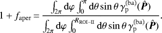 (A.9)
(A.9)
Typically, faper ~ 10−3; they are listed in Table 1.
A.7 Beam model efficiency
The integralover 4π of an ideal beam model must be normalized to some reference value, which is usually either 1 or 4π. However, real models computed with GRASP suffer numerical errors giving a slightly smaller results than the reference value. These numerical errors have many origins; the most important are the spatial resolution of the beam pattern, and the order of the approximation used by GRASP to propagate the electromagnetic field through the telescope. The effect has a magnitude of some 10−3 and its value for each radiometer is reported in Table 1, column fη. The quantity fη is defined as
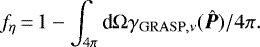 (A.10)
As this effect resembles a power loss in the beam, we dubbed fη as beam model efficiency.
There are two possible corrections to this effect. Firstly, we could assume that the GRASP model is the correct beam model scaled by 1 − fη. In this case,  is not affected by the beam model efficiency, but the measured ΔTant,p is scaled up by a systematic factor 1∕(1 − fη). This was the assumption used in Planck Collaboration V (2016). The problem with this approach is that the systematic effect leading to fη≠0 is supposed to be equally distributed between the main beam and the side lobes. However, a GRASP model is built to reproduce beam maps obtained from bright point sources, which are primarily sensitive to the shape of the main beam. Therefore, the cause for fη≠0 is likely in the side-lobe pattern, which cannot be easily constrained by observations. In this case
  is unaffected by the problem, but the value of
  that has been derived from the model is erroneously scaled down by 1 − fη.
Blocking corrections as antenna temperatures.
The truth is likely somewhere in the middle, and the measured brightness must be corrected by an unknown factor 1 + x, with − fη ≤ x ≤ +fη. As we could not tell what is the proper correction to apply, we avoided this step and left it as a source of uncertainty with a flat distribution in the range [−fη, fη]. Appendix A.12 provides more details of how this is accounted for in Monte Carlo simulations and bootstrap analyses.
Because it is a systematic effect, this error should be quoted separately as an unknown scaling factor applied to Bp, Tb,rj, Tb,c, or  . However, if we are estimating a total uncertainty budget, it is possible to consider this error as a random value with variance
  , which can be added to the noise variance. This is clear in the analysis of Bp, Tb,rj, Tb,c or
  derived from Monte Carlo simulations and bootstrap methods. A more conservative approach would be to drop the 1∕3 factor and simply add
  to the variance.
A.8 Side lobes
It is customary to include only the main beam in the value of Ωbeam. Correction for the power spilled in the side lobes is usually accounted with a term 1 + fSL that corrects for the side-lobe efficiency (Planck Collaboration V 2014, 2016). In this work, we do not follow this convention as we integrated  over the whole 4π sphere; therefore, no fSL correction is needed.
A.9 Blocking
Blocking can be considered as a negative contribution to brightness, as in Eq. (26), or as a correction on the brightness temperature. The former quantity is listed in Table 1, in Table A.2 we provide the corresponding antenna temperatures.
A.10 ( )cmb
)cmb
The  factor is used to convert the antenna temperature ΔTant,p into a brightness, like in Eq. (21). The assumption that the CMB spectrum follows the RJ law, (
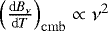 ), leads to overestimating the brightness of ≈12% at 70 GHz, 5% at 44 GHz, and 2.2% at 30 GHz. Replacing
  with
with  has the effect of slightly underestimating the brightness of 4.5 × 10⁻³−6.9 × 10⁻³ at 30 GHz, 2.1 × 10⁻³−3.2 × 10⁻³ at 44 GHz, and1.7 × 10−3−3.6 × 10⁻³ at 70 GHz.
A.11 Band averaged Bν
To solve for  from Eq. (29), we exploit the fact that
  is a nearly linear increasing function of Tb. For each radiometer, we tabulate the quantity
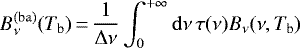 (A.11)
for 10 K ≤ Tb ≤ 500 K in steps of 1 K. The tabulated function is then inverted by interpolating Tb as a function of measured Bp, using the right side of Eq. (29) as input.
It is interesting to compare the difference in Tb accounting for band averaging versus simple analytical inversion of Bp = Bν(νcent, Tb). For this, we can define a further correction factor  . In all the cases, fTbBa < 0: this means that neglecting band averaging causes an overestimation of Tb. The quantity fTbBa varies between 3.9 × 10⁻³ and 8.2 × 10⁻³, depending on the radiometer. Differences in brightness temperatures are between − 1.5 K and − 0.5 K, depending on the radiometer and the planet. Different planets and/or transits alter fTbBa by less than 10−5.
A.12 Averaged values
There are various ways to compute averaged values from our list of measurements Bp, Tb,rj, Tb,c and  for a planet from each transit and radiometer. The simplest method is to compose a subset of measurements specifying a list of transits and radiometers belonging to a given frequency channel and then to derive the weighted average of Bp, Tb,rj, Tb,c, and
  . This is the approach used in Planck Collaboration V (2016), where channel averages were computed and then averaged across the transits. The final uncertainty
  of
of  can be derived analytically using error propagation; however, if the distribution of x is not Gaussian, then unreasonably small
  are obtained. A better approach is to follow a least-squares minimization, fitting
  to the list of xi in the subset
 (A.12)
where x is either Bp, Tb,rj, Tb,c, or  , and σi is the uncertainty. As is well known, the minimization of χ2 gives the weighted average formula, but the use of numerical minimization codes, such as the curve_fit function in the SciPy package (Virtanen et al. 2020), can estimate
  from the covariance matrix of errors of fitted parameters, leading to a more prudent estimate of the uncertainty.
Alternatively, a bootstrap of fitting residuals  can be used to resample the input xi, and to derive a distribution of possible values of
  from which
  can be obtained. In this case, we used the bootstrap algorithm provided by the scikit-learn package (Pedregosa et al. 2011). Finally by defining a likelihood for
  :
:  and a prior for
  , a posterior probability for
  can be formed and maximized. Uncertainties can be estimated with Monte Carlo simulations.
In this paper we follow all of those approaches to define the uncertainties of our estimated averaged values, employing emcee (Foreman-Mackey et al. 2013) for the estimation of uncertainties using Monte Carlo simulations. In general the results of the three methods are consistent each other, but in some cases the bootstrap approach provided larger uncertainties. We chose to take the largest uncertainty provided by the three methods for each averaged quantity.
Since Tb,c and  are not additive quantities like Bp and Tb,rj, we estimated
  through the minimization of the quantity
  , defined as
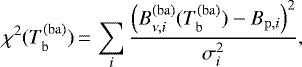 (A.13)
where σi is the uncertainty on the measured Bp,i, and  is the black-body emissivity averaged over the bandpass for the radiometer that acquired the ith sample. The application of the bootstrap method requires to sample the residuals
  . The application of the MCMC method requires to define the likelihood
 (A.14)
which constrains  . Similar formulas can be derived for Tb,c by replacing
  with Bν(νcent,i, T), where νcent,i is the central frequency of sample i.
To investigate the effect of the uncertainty in the correction for the beam numerical efficiency described in Appendix A.7, we redefined the bootstrapped simulated brightness for sample i as
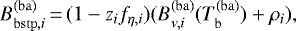 (A.16)
where {ρi} is a list of residuals sampled from the distribution of {ri}, {zi } is a list of random numbers taken from the uniform distribution [−1, 1]. Similarly, toinvestigate this effect using a Monte Carlo simulation we modified the likelihood in Eq. (A.14) by replacing  with
with  , where {zi } is a set of parameters with a flat distribution
 (A.17)
which multiplies the prior distribution for  .
.
Since we are dealing with averaged quantities, we had to define a reference frequency. For each subset of measurements we took the weighted average of the νcent of each measure, using the σi as weights. As the relative errors for Bp, Tb,rj, Tb,c, and  are similar, the resulting averaged νcent is nearly independent on the choice of the quantity to be averaged.
A.13 Conversion of T to Tb
to Tb
The WMAP collaboration provided planets brightness temperatures in form of Tb,rj and without any correction for blocking (e.g., Weiland et al. 2011). To properly compare WMAP results to models, Tb,rj must be converted either to Tb,c or  . In addition we must take in account the different value of the dipole amplitude used by Planck and WMAP, as this leads to a mismatch in the absolute calibration level. The Planck team used the value APlanck = 3364 ± 2 μK (Planck Collaboration V 2014, 2016; Planck Collaboration II 2020), while the WMAP team used AWMAP = 3355 ± 8 μK (Hinshaw et al. 2009). Therefore, we scaled the WMAP estimates of Tb,rj by a factor of GWMAP,Planck = 1.002831 ± 0.00246.

where ΔTant,block is provided by Page et al. (2003) for the bands K, Ka, Q, V, and W assuming values 2.2, 2, 1.9, 1.5 and 1.1 K respectively. We note that both Bν,rj,1(ν) and Bν (ν, T) depend on frequency; we evaluated them at the central frequencies of each band as defined in Table 3 of Weiland et al. (2011).
For  , we follow what we explained in Appendix A.11 and solve for
 (A.19)
where the bandpass τ(ν) for each band is taken from the Lambda website17.
We note that other authors such as Gibson et al. (2005) and Karim et al. (2018) convert Tb,rj to Tb,c applying an additive correction defined as follows:
 (A.20)
where ΔTrj→b is equal to 0.54, 0.79, 0.98, 1.46 and 2.23 K for the bands from K to W; this is because of the assumption that  shows only a slight dependence on T for ν < 100 GHz and T > 100 K. In this work however we prefer to apply Eq. (A.13).
Finally, we want to underline the fact that the concise descriptions usually reported in the literature for this conversion leave some ambiguity in reproducing the published results. An example is Table 2 from Gibson et al. (2005). The authors quoted Page et al. (2003) and reported the value Tb,rj = 146.6 K, but after the application of several corrections they end with a new estimate Tb,rj = 147.8 K that is converted in their final  by adding 0.79 K. However, the 0.79 K correction is the difference Tb,c,(Ka)(148.4 K) − 148.4 K that is derived from Eq. (A.18), and not the difference
  from Eq. (A.19), which is 0.23 K. The authors state that they converted Tb,rj to Tb through the integration of a black-body ideal brightness over the WMAP bandpass. The difference is negligible when compared to the final uncertainties, so that the conclusions in Gibson et al. (2005) and Karim et al. (2018) (as well as other papers that apply the same procedure) are not affected at all. But without the possibility to reconstruct the exact conversion procedure followed by other authors, it is difficult to judge whether small differences between our results and their results are significant or not.
A.14 T and Tb,rj relations
It might sound surprising that  for 70 GHz and 44 GHz data, while
  for 30 GHz data. However, this is expected and is mainly a consequence of the interplay of bandwidth and Planck’s law.
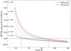 |
Fig. A.1 Ratio |

Let us assume that we are observing a source with brightness  . Then, Tb,rj, Tb,c, and
  are solutions of the equations
  and
and  . Given some temperature T, if
  then
then  , and vice versa. We model bandpasses as top-hat functions with τ(ν) = 1 in the frequency range νcent − δ∕2 ≤ ν ≤ νcent + δ∕2 and zero otherwise. However, to better model the nuances of the Planck/LFI bandpasses, instead of using Δ to characterize the bandwidth, we use the parameter q, defined as follows:
 (A.21)
which reduces to  for a top-hat bandpass. With those conventions, whenever the RJ approximation and Planck’s law agree, it follows that
 (A.22)
Given that the bandpass is symmetrical and receives more contribution from the high-frequency side, the band-averaged brighntess is larger than the monocromatic RJ. Consequently, in this approximation  . However as νcent increases, the RJ approximation overestimates the true black-body brightness. Because of this, above some central frequency νcent,1 we must have
  and
and  . The derivation of an approximated expression for νcent,1 is based on the factorization of Planck’s law as the product of the RJ law and a dumping factor x∕(ex − 1) with x = hν∕kbT. Given that we are in the limits of small x with a much smaller δ, we may assume that over the bandpass x∕(ex − 1) ≈ xc∕(exc − 1) ≈ 1∕(1 + xc∕2), where xc = hνcent∕kbT. Therefore, the band-averaged brightness has again the form of the right side of Eq. (A.22), but scaled by the factor x∕(ex − 1). The critical frequency is such that
  , and therefore
![\begin{equation*}\nu_{\mathrm{cent},1} \approx \sqrt[3]{\frac{2k_{\mathrm{b}} T}{h}} q^{2/3}; \end{equation*}](/articles/aa/full_html/2021/03/aa37788-20/aa37788-20-eq232.png) (A.23)
(A.23)
if T is expressed in K and q in GHz, then νcent,1 ≈ 3.47 T1∕3q2∕3 GHz. A representative case for Planck/LFI observations of Jupiter is T = 150 K and q in the range 1 GHz–6.5 GHz, resulting in νcent,1 in the range 18–64 GHz. A more accurate calculation can be easily obtained numerically, and this is shown in Fig. A.1, where the ratio  is calculated for the representative case T = 150 K. As expected from our calculation, since the dumping factor decreases with νcent, the ratio of the band-averaged brightness to the RJ brightness decreases too; the main parameter describing the curve is q. For radiometer 27S, q ≈ 2.4 GHz: in fact, the corresponding line fits nicely between the top-hat bandpasses with q = 2 GHz and q = 3 GHz. We find a similar behaviour for 18S, where q ≈ 6.5 GHz.
Effective bandwidth q and critical central frequency νcent,1.
For the Planck/LFI radiometers, νcent,1 always falls within the range 29.1–66.5 GHz. In particular for the 27S, we derive numerically νcent,1 = 29.2 GHz, while the analytical approximation gives 30 GHz. For the 18S, we derive 63.5 GHz numerically and 64 GHz analytically.
The explanation of the inverted behaviour of  and Tb,rj at 30 GHz and at 70 GHz is now clear. For 27S, νcent = 28.5 GHz, just below its critical value, so for this channel
  and
and  . On the contrary, for 18S νcent = 70.1 GHz, slightly above its critical value: this results in
  and
and  . Last but not least, the 44 GHz radiometers have q comparable to those of the 30 GHz, since νcent,1 ≈ 30 GHz, smaller than their central frequencies: therefore, they behave as the 70 GHz radiometers.
Table A.3 provides the estimates for q and νcent,1 for all the Planck/LFI radiometers. We computed the values for νcent,1 by numerical integration at the reference temperature of 150 K. These values can be scaled to different temperatures in the range 125–175 K by using the![$\sqrt[3]{T}$](/articles/aa/full_html/2021/03/aa37788-20/aa37788-20-eq239.png) dependence of Eq. (A.23) within a two percent accuracy.
dependence of Eq. (A.23) within a two percent accuracy.
References
- Astropy Collaboration (Robitaille, T. P., et al.) 2013, A&A, 558, A33 [NASA ADS] [CrossRef] [EDP Sciences] [Google Scholar]
- Astropy Collaboration (Price-Whelan, A. M., et al.) 2018, AJ, 156, 123 [Google Scholar]
- Ben-Reuven, A. 1966, Phys. Rev., 145, 7 [CrossRef] [Google Scholar]
- Bendo, G. J., Griffin, M. J., Bock, J. J., et al. 2013, MNRAS, 433, 3062 [NASA ADS] [CrossRef] [Google Scholar]
- Bennett, C. L., Larson, D., Weiland, J. L., et al. 2013, ApJS, 208, 20 [Google Scholar]
- Bertincourt, B., Lagache, G., Martin, P. G., et al. 2016, A&A, 588, A107 [NASA ADS] [CrossRef] [EDP Sciences] [Google Scholar]
- BeyondPlanck Collaboration 2020, BeyondPlanck I. Global Bayesian analysis of the Planck Low Frequency Instrument data [Google Scholar]
- Cunningham, C. T., Ade, P. A. R., Robson, E. I., Nolt, I. G., & Radostitz, J. V. 1981, Icarus, 48, 127 [Google Scholar]
- de Pater I. 1981, A&A, 93, 370 [Google Scholar]
- de Pater I. 2018, Nat. Astron., 2, 364 [Google Scholar]
- de Pater, I., & Dickel, J. R. 1991, Icarus, 94, 474 [NASA ADS] [CrossRef] [Google Scholar]
- de Pater, I., & Dunn, D. E. 2003, Icarus, 163, 449 [NASA ADS] [CrossRef] [Google Scholar]
- de Pater, I., & Massie, S. T. 1985, Icarus, 62, 143 [Google Scholar]
- de Pater, I., & Mitchell, D. L. 1993, J. Geophys. Res., 98, 5471 [Google Scholar]
- de Pater, I., & Richmond, M. 1989, Icarus, 80, 1 [NASA ADS] [CrossRef] [Google Scholar]
- de Pater, I., Kenderdine, S., & Dickel, J. R. 1982, Icarus, 51, 25 [NASA ADS] [CrossRef] [Google Scholar]
- de Pater, I., Romani, P. N., & Atreya, S. K. 1991, Icarus, 91, 220 [NASA ADS] [CrossRef] [Google Scholar]
- de Pater, I., Heiles, C., Wong, M., et al. 1995, Highlights Astron., 10, 637 [Google Scholar]
- de Pater, I., Fletcher, L. N., Luszcz-Cook, S., et al. 2014, Icarus, 237, 211 [NASA ADS] [CrossRef] [Google Scholar]
- de Pater, I., Sault, R. J., Butler, B., DeBoer, D., & Wong, M. H. 2016, Science, 352, 1198 [NASA ADS] [CrossRef] [Google Scholar]
- de Pater, I., Butler, B., Sault, R. J., et al. 2018, ASP Conf. Ser., 517, 49 [Google Scholar]
- de Pater, I., Sault, R. J., Moeckel, C., et al. 2019a, AJ, 158, 139 [NASA ADS] [CrossRef] [Google Scholar]
- de Pater, I., Sault, R. J., Wong, M. H., et al. 2019b, Icarus, 322, 168 [Google Scholar]
- Dunn, D. E., Molnar, L. A., & Fix, J. D. 2002, Icarus, 160, 132 [NASA ADS] [CrossRef] [Google Scholar]
- Dunn, D. E., de Pater, I., & Sault, R. J. 2003, Icarus, 165, 121 [NASA ADS] [CrossRef] [Google Scholar]
- Dunn, D. E., de Pater, I., Wright, M., Hogerheijde, M. R., & Molnar, L. A. 2005, AJ, 129, 1109 [Google Scholar]
- Encrenaz, T., & Moreno, R. 2002, AIP Conf. Ser., 616, 330 [Google Scholar]
- Epstein, E. E., Janssen, M. A., Cuzzi, J. N., Fogarty, W. G., & Mottmann, J. 1980, Icarus, 41, 103 [NASA ADS] [CrossRef] [Google Scholar]
- Foreman-Mackey, D., Hogg, D. W., Lang, D., & Goodman, J. 2013, PASP, 125, 306 [Google Scholar]
- Gibson, J., Welch, W. J., & de Pater, I. 2005, Icarus, 173, 439 [Google Scholar]
- Goldin, A. B., Kowitt, M. S., Cheng, E. S., et al. 1997, ApJ, 488, L161 [NASA ADS] [CrossRef] [Google Scholar]
- Górski, K. M., Hivon, E., Banday, A. J., et al. 2005, ApJ, 622, 759 [NASA ADS] [CrossRef] [Google Scholar]
- Greve, A., Steppe, H., Graham, D., & Schalinski, C. J. 1994, A&A, 286, 654 [Google Scholar]
- Griffin, M. J., & Orton, G. S. 1993, Icarus, 105, 537 [Google Scholar]
- Griffin, M. J., North, C. E., Schulz, B., et al. 2013, MNRAS, 434, 992 [NASA ADS] [CrossRef] [Google Scholar]
- Grossman, A. W., Muhleman, D. O., & Berge, G. L. 1989, Science, 245, 1211 [Google Scholar]
- Gulkis, S., Janssen, M. A., & Olsen, E. T. 1978, Icarus, 34, 10 [NASA ADS] [CrossRef] [Google Scholar]
- Hazumi, M., Ade, P. A. R., Akiba, Y., et al. 2019, J. Low Temp. Phys., 194, 443 [Google Scholar]
- Hinshaw, G., Weiland, J. L., Hill, R. S., et al. 2009, ApJS, 180, 225 [NASA ADS] [CrossRef] [Google Scholar]
- Hunter, J. D. 2007, Comput. Sci. Eng., 9, 90 [NASA ADS] [CrossRef] [Google Scholar]
- Janssen, M. A., & Olsen, E. T. 1978, Icarus, 33, 263 [Google Scholar]
- Janssen, M. A., Ingersoll, A. P., Allison, M. D., et al. 2013, Icarus, 226, 522 [Google Scholar]
- Joiner, J., & Steffes, P. G. 1991, J. Geophys. Res., 96, 17, 463 [Google Scholar]
- Karim, R. L., DeBoer, D., de Pater, I., & Keating, G. K. 2018, AJ, 155, 129 [Google Scholar]
- Keihänen, E., Kurki-Suonio, H., Poutanen, T., Maino, D., & Burigana, C. 2004, A&A, 428, 287 [NASA ADS] [CrossRef] [EDP Sciences] [Google Scholar]
- Klein, M. J., & Gulkis, S. 1978, Icarus, 35, 44 [Google Scholar]
- Klein, M. J., & Hofstadter, M. D. 2006, Icarus, 184, 170 [NASA ADS] [CrossRef] [Google Scholar]
- Klein, M. J., Janssen, M. A., Gulkis, S., & Olsen, E. T. 1978, NASA Conference Publication, 2068, 195 [Google Scholar]
- Klein, M. J., Bolton, S. J., Gulkis, S., et al. 2001, Planetary Radio Emissions V, 221 [Google Scholar]
- Kloosterman, J. L., Dunn, D. E., & de Pater, I. 2005, ApJS, 161, 520 [NASA ADS] [CrossRef] [Google Scholar]
- Kramer, C., Moreno, R., & Greve, A. 2008, A&A, 482, 359 [NASA ADS] [CrossRef] [EDP Sciences] [Google Scholar]
- Lellouch, E., & Destombes, J. L. 1985, A&A, 152, 405 [Google Scholar]
- Maino, D., Burigana, C., Górski, K. M., Mandolesi, N., & Bersanelli, M. 2002, A&A, 387, 356 [NASA ADS] [CrossRef] [EDP Sciences] [Google Scholar]
- Maris, M., & Burigana, C. 2009, Earth Moon Planets, 105, 81 [Google Scholar]
- McKinney, W. 2010, Proceedings of the 9th Python in Science Conference, eds. S. van der Walt, & J. Millman, 51 [Google Scholar]
- Mennella, A., Bersanelli, M., Butler, R. C., et al. 2010, A&A, 520, A5 [NASA ADS] [CrossRef] [EDP Sciences] [Google Scholar]
- Moreno, R. 1998, PhD thesis, Universite Paris VI, Paris [Google Scholar]
- Muhleman, D. O., & Berge, G. L. 1991, Icarus, 92, 263 [Google Scholar]
- Müller, T. G., Balog, Z., Nielbock, M., et al. 2016, A&A, 588, A109 [NASA ADS] [CrossRef] [EDP Sciences] [Google Scholar]
- Orton, G. S., Fletcher, L. N., Moses, J. I., et al. 2014, Icarus, 243, 494 [NASA ADS] [CrossRef] [Google Scholar]
- Page, L., Barnes, C., Hinshaw, G., et al. 2003, ApJS, 148, 39 [NASA ADS] [CrossRef] [Google Scholar]
- Pedregosa, F., Varoquaux, G., Gramfort, A., et al. 2011, J. Mach. Learn. Res., 12, 2825 [Google Scholar]
- Pérez, F., & Granger, B. E. 2007, Comput. Sci. Eng., 9, 21 [Google Scholar]
- Planck Collaboration I. 2014, A&A, 571, A1 [NASA ADS] [CrossRef] [EDP Sciences] [Google Scholar]
- Planck Collaboration III. 2014, A&A, 571, A3 [NASA ADS] [CrossRef] [EDP Sciences] [Google Scholar]
- Planck Collaboration IV. 2014, A&A, 571, A4 [NASA ADS] [CrossRef] [EDP Sciences] [Google Scholar]
- Planck Collaboration V. 2014, A&A, 571, A5 [NASA ADS] [CrossRef] [EDP Sciences] [Google Scholar]
- Planck Collaboration III. 2016, A&A, 594, A3 [NASA ADS] [CrossRef] [EDP Sciences] [Google Scholar]
- Planck Collaboration IV. 2016, A&A, 594, A4 [NASA ADS] [CrossRef] [EDP Sciences] [Google Scholar]
- Planck Collaboration V. 2016, A&A, 594, A5 [NASA ADS] [CrossRef] [EDP Sciences] [Google Scholar]
- Planck Collaboration I. 2020, A&A 641, A1 [CrossRef] [EDP Sciences] [Google Scholar]
- Planck Collaboration II. 2020, A&A 641, A2 [CrossRef] [EDP Sciences] [Google Scholar]
- Planck Collaboration Int. LII. 2017, A&A, 607, A122 [NASA ADS] [CrossRef] [EDP Sciences] [Google Scholar]
- Santos-Costa, D., Bolton, S. J., Sault, R. J., Thorne, R. M., & Levin, S. M. 2011, J. Geophys. Res Space Phys., 116, A12236 [Google Scholar]
- Schloerb, F. P., Muhleman, D. O., & Berge, G. L. 1979a, Icarus, 39, 214 [NASA ADS] [CrossRef] [Google Scholar]
- Schloerb, F. P., Muhleman, D. O., & Berge, G. L. 1979b, Icarus, 39, 232 [Google Scholar]
- Teyssier, D., & Marston, A. 2017, Release notes: Herschel Planetary Calibrator models, Tech. Rep. 1-0, ESA [Google Scholar]
- Tollefson, J., de Pater, I., Luszcz-Cook, S., & DeBoer, D. 2019, AJ, 157, 251 [Google Scholar]
- van der Tak, F., de Pater, I., Silva, A., & Millan, R. 1999, Icarus, 142, 125 [Google Scholar]
- Virtanen, P., Gommers, R., Oliphant, T. E., et al. 2020, Nat. Methods, 17, 261 [Google Scholar]
- Weiland, J. L., Odegard, N., Hill, R. S., et al. 2011, ApJS, 192, 19 [Google Scholar]
- Zonca, A., Singer, L., Lenz, D., et al. 2019, J. Open Source Softw., 4, 1298 [NASA ADS] [CrossRef] [Google Scholar]

Results from de Pater et al. (1982) and Goldin et al. (1997) are not included, as they are outside the frequency range of interest.
Data presented in Schloerb et al. (1979a), Epstein et al. (1980), Cunningham et al. (1981) and Grossman et al. (1989) are outside our frequency range.
Data from Cunningham et al. (1981), Griffin & Orton (1993) and Klein & Hofstadter (2006) are not shown here since they are outside the frequency range of interest.
Usually, analysis of planets assumes that a planet has a well-defined radius (i.e., the planet is a solid object). For a gas giant this is not true, since limb darkening and brightness temperature distribution across layers makes the radius a function of ν, so that different instruments with different bandpass see different Ωp. Analysis of this problem is postponed to another paper.
In Planck Collaboration V (2014), the fiducial Ωp was taken at the pole.
All Tables
All Figures
|
Fig. 1 Geometrical configuration of a planet observation by Planck. Left and right frames: trailing and leading observations respectively. The position of the spacecraft is denoted by RS, the position of the planet by Rpl. The Sun is indicated with the symbol ⊙. Both the spacecraft and the planet revolve counter-clockwise around the Sun in circular and coplanar orbits. For a detailed discussion of the symbols, see the text. |
| In the text | |
|
Fig. 2 Time dependence of the angle between Jupiter’s direction and the spin axis of the Planck spacecraft. The darker horizontal bar indicates the angular region of the 11 LFI beam axes, while the lighter bar is enlarged by ± 5°. Saturn, Uranus, and Neptune show a similar pattern. The labels SS1…SS8 denote Planck sky surveys, as defined in Planck Collaboration V (2016), from which the figure is taken. Tr1…Tr7 denote the transits; letters T and L indicate whether it was a trailing or leading transit, according to Fig. 1. |
| In the text | |
|
Fig. 3 Example of a map in the (u, v) reference frame for Jupiter. This image shows the first transit as seen by radiometer 27–0 (30 GHz). Top left: map of Tant in Kcmb ranging from − 4 × 10⁻⁴ Kcmb to 0.4 Kcmb. Top right: map of the background model, expressed as Tant in Kcmb ranging from − 4 × 10⁻⁴ Kcmb to 1 × 10⁻³ Kcmb. Bottom left: histogram of Tant in Kcmb for the background. The green points indicate the samples in the histogram, the red line indicates the best-fit Gaussian distribution,and the threshold for the classification mask is shown by the dashed blue line. Bottom right: classification mask. The grey region shows the planet ROI, the white annulus is the background ROI, and the blue regions denote unused samples. |
| In the text | |
|
Fig. 4 Antenna temperature estimates Tant for Jupiter, Saturn, Uranus, and Neptune (top to bottom) and for three radiometers representative of the 30 GHz (left), 44 GHz (centre), and 70 GHz (right) channels, as a function of the angular distance from the beam centre. The blue bands show the distribution of samples in the planet ROI (dark blue: 1σ region; light blue: peak-to-peak variation). The green bands have the same interpretation, but indicate the background ROI. The grey bands show the data before having been σ-clipped; for the case of Saturn observed by LFI27-0 a point source is present that was removed before the analysis (not present in the green line). The separation between the blue and green lines indicates the presence of the avoidance ROI, not included in our fits. The red line shows the best-fit model, and its width is the root mean square (RMS) of the model due to the ellipticity of the beam. |
| In the text | |
|
Fig. 5 Radial pattern of residuals averaged over the whole set of transits. |
| In the text | |
|
Fig. 6 Values of |
| In the text | |
|
Fig. 7 Values of ΔTant,p after reduction to fiducial observing conditions and standardized Ωbeam and Ωp. |
| In the text | |
|
Fig. 8 Values of channel-averaged |
| In the text | |
|
Fig. 9 Comparison of Jupiter measurements made in this paper (red circles) with WMAP (black points, taken from Weiland et al. (2011); Bennett et al. (2013) and converted to
|
| In the text | |
|
Fig. 10 Saturn Tb,rj for 70 GHz frequency channel (first frame from top), 44 GHz frequency channel (second and third frames), and 30 GHz frequency channel (fourth frame) as a function of DP. Labels Tr1, Tr2, …, Tr8 denotes the transit from which each observation originates. Continuous curves refers to the best-fit models of Tb with various selections of data: all transits, transits 7 and 8 excluded, and transits 3, 7, and 8 excluded. The grey bands are 1σ uncertainties in the models. |
| In the text | |
|
Fig. 11 Spectral energy distribution of Saturn rings from Planck/LFI (red), Planck/HFI (blue), and WMAP (black). Data from previous literature outside WMAP and Planck are shown in light grey (references in the text). |
| In the text | |
|
Fig. 12 Spectral energy distribution of Saturn disc from Planck/LFI (red), Planck/HFI (blue) and WMAP (black). The model labelled dePater and Mitchel (1993,A) does not include clouds, while dePater and Mitchel (1993,D) includes clouds. For other details about the other models, see the text. |
| In the text | |
|
Fig. 13
|
| In the text | |
|
Fig. A.1 Ratio |
| In the text | |
Current usage metrics show cumulative count of Article Views (full-text article views including HTML views, PDF and ePub downloads, according to the available data) and Abstracts Views on Vision4Press platform.
Data correspond to usage on the plateform after 2015. The current usage metrics is available 48-96 hours after online publication and is updated daily on week days.
Initial download of the metrics may take a while.