| Issue |
A&A
Volume 637, May 2020
|
|
|---|---|---|
| Article Number | A58 | |
| Number of page(s) | 23 | |
| Section | Extragalactic astronomy | |
| DOI | https://doi.org/10.1051/0004-6361/202037506 | |
| Published online | 14 May 2020 | |
The chemical evolution of galaxy clusters: Dissecting the iron mass budget of the intracluster medium
1
INAF – Osservatorio Astrofisico di Arcetri, Largo E. Fermi, 50125 Firenze, Italy
e-mail: This email address is being protected from spambots. You need JavaScript enabled to view it.
, This email address is being protected from spambots. You need JavaScript enabled to view it.
2
Department of Physics, Sapienza University of Rome, 00185 Rome, Italy
3
Department of Physics, University of Rome Tor Vergata, 00133 Rome, Italy
4
INAF – Osservatorio di Astrofisica e Scienza dello Spazio, Via Pietro Gobetti 93/3, 40129 Bologna, Italy
5
INFN, Sezione di Bologna, Viale Berti Pichat 6/2, 40127 Bologna, Italy
6
INAF – Osservatorio Astronomico di Brera, Via E. Bianchi, 46, 23807 Merate, LC, Italy
7
INAF – Istituto di Astrofisica Spaziale e Fisica cosmica di Milano, Italy
8
Dipartimento di Fisica e Scienze della Terra, Universitá degli Studi di Ferrara, Via Saragat 1, 44122 Ferrara, Italy
9
Department of Physics and Astronomy, Johns Hopkins University, 3400 N. Charles Street, Baltimore, MD 21218, USA
Received:
14
January
2020
Accepted:
26
March
2020
Abstract
Aims. We study the chemical evolution of galaxy clusters by measuring the iron mass in the ICM after dissecting the abundance profiles into different components.
Methods. We used Chandra archival observations of 186 morphologically regular clusters in the redshift range of [0.04, 1.07]. For each cluster, we computed the azimuthally averaged iron abundance and gas density profiles. In particular, our aim is to identify a central peak in the iron distribution, which is associated with the central galaxy, and an approximately constant plateau reaching the largest observed radii, which is possibly associated with early enrichment that occurred before or shortly after achieving virialization within the cluster. We were able to firmly identify two components in the iron distribution in a significant fraction of the sample simply by relying on the fit of the iron abundance profile. From the abundance and ICM density profiles, we computed the iron mass included in the iron peak and iron plateau, and the gas mass-weighted iron abundance of the ICM out to an extraction radius of 0.4r500 and to r500 by extending the abundance profile as a constant.
Results. We find that the iron plateau shows no evolution with redshift. On the other hand, we find a marginal (< 2σ c.l.) decrease with redshift in the iron mass included in the iron peak rescaled by the gas mass. We measure that the fraction of iron peak mass is typically a few percent (∼1%) of the total iron mass within r500. Therefore, since the total iron mass budget is dominated by the plateau, we find consistently that the global gas mass-weighted iron abundance does not evolve significantly across our sample. We were also able to reproduce past claims of evolution in the global iron abundance, which turn out to be due to the use of cluster samples with different selection methods combined with the use of emission-weighted, instead of gas mass-weighted, abundance values. Finally, while the intrinsic scatter in the iron plateau mass is consistent with zero, the iron peak mass exhibits a large scatter, in line with the fact that the peak is produced after the virialization of the halo and depends on the formation history of the hosting cool core and the strength of the associated feedback processes.
Conclusions. We conclude that only a spatially resolved approach can resolve the issue of iron abundance evolution in the ICM, reconciling the contradictory results obtained in the last ten years. Evolutionary effects below z ∼ 1 are marginally measurable with present-day data, while at z > 1 the constraints are severely limited by poor knowledge of the high-z cluster population. The path towards a full and comprehensive chemical history of the ICM requires the application of high angular resolution X-ray bolometers and a dramatic increase in the number of faint, extended X-ray sources.
Key words: galaxies: clusters: general / galaxies: clusters: intracluster medium / X-rays: galaxies: clusters
© ESO 2020
1. Introduction
Massive galaxy clusters (M500 > 1014 M⊙) are thought of as closed boxes that retain the past history of their cosmic evolution. The majority of their total mass takes the form of dark matter, which contributes 80–90% of the mass budget. While the stellar mass in member galaxies or in a diffuse component only constitutes a minor fraction (about 1–2% of the total and 6–12% of the baryonic mass; see Lin et al. 2012), the baryonic mass is dominated by the intracluster medium (ICM), which is a hot, optically-thin diffuse plasma at low densities in a local collisional equilibrium with temperatures of the order of 107 to 108 K. The thermodynamical and dynamical status of the ICM is non-trivially linked to the mass accretion history of the dark matter halo, the nuclear feedback from the central galaxy, and the star formation processes in the member galaxies. The latter, in particular, leaves its imprint on the ICM as a widespread chemical enrichment of heavy elements, mostly produced by supernovae explosions in the member galaxies, which can be efficiently measured with X-ray spectroscopy (Böhringer & Werner 2010; Mernier et al. 2018); this finding is also supported by relevant simulations (see Biffi et al. 2018a, and references therein). Tracing the evolution of metal abundance in the ICM can therefore provide useful information for revealing the star-formation history in cluster galaxies across cosmic time and the process that led to to the mixing of the intergalactic medium (IGM) with the ICM (Böhringer et al. 2004; de Plaa 2013).
The abundance of heavy elements (also generically referred to as “metals”) in the ICM can be measured through the equivalent width of their emission lines in the X-ray spectrum. In particular, iron is the element with the most prominent emission features and it is therefore the only heavy element that has been detected in galaxy clusters up to z ∼ 1.6 and possibly up to z ∼ 2 (Rosati et al. 2009; Tozzi et al. 2013, 2015; Mantz et al. 2018) thanks to the Kα emission line complex at 6.7–6.9 keV. The detection of other metals, instead, typically requires high signal-to-noise (S/N) spectra and is therefore basically limited to lower temperatures (kT < 3 keV), low redshifts, and central regions (De Grandi & Molendi 2009; Tamura et al. 2009; Mernier et al. 2017). In this framework, iron is the only element that can be robustly used to investigate the spatial distribution in the ICM and the cosmic evolution of metals on a timescale of ∼10 Gyr.
Several attempts have been made in the past decades to derive an average cosmic evolution of iron abundance in the ICM. Following the first attempts (e.g., Mushotzky & Loewenstein 1997; Tozzi et al. 2003), the first reliable assessment of the cosmic evolution of iron abundance in the ICM were obtained about ten years ago thanks to the exploitation of Chandra and XMM-Newton archives. These works suggested a statistically significant evolution of a factor of 2 in the redshift range 0 < z < 1.3 (Balestra et al. 2007; Maughan et al. 2008; Anderson et al. 2009). The picture became less clear over recent years, when new analyses showed little or no evolution (Ettori et al. 2015; McDonald et al. 2016). In addition, spatially resolved analysis adds further complications: the results are not only influenced by the radial range used to measure the abundance (Baldi et al. 2012; Mantz et al. 2017), but they also change significantly when using SZ-selected samples of clusters, instead of the former X-ray selected clusters (see, e.g., McDonald et al. 2016). Moreover, several works have shown that the spatial distribution of iron in the central regions evolves significantly with time (De Grandi et al. 2014), despite the fact that this does not necessarily imply a change in the amount of metals in the ICM, but rather a simple redistribution (Liu et al. 2018). As a consequence, a measurement of iron abundance without a resolution of its spatial distribution can potentially introduce systematic uncertainties as high as ∼25% (Liu et al. 2018). A further critical aspect is that very little is known about the distribution of metals at large radii, so statistical studies are meaningful only for radii below r500 (Molendi et al. 2016).
We argue that in order to reach a clearer picture of the evolution of iron in the ICM on the basis of current X-ray data archives, we should efficiently exploit what we know about the iron distribution. Both simulations and observations have indicated that the spatial distribution of iron in the ICM often appears to be well described as a combination of two main components: a peak in the inner regions, which is usually centered on the brightest cluster galaxy (BCG), and a large-scale component with abundance across the cluster that is either approximately uniform (De Grandi & Molendi 2001; Baldi et al. 2007; Leccardi & Molendi 2008; Sun et al. 2009; Simionescu et al. 2009, 2017; Werner et al. 2013; Thölken et al. 2016; Urban et al. 2017; Lovisari & Reiprich 2019) or slightly decreasing (e.g., Mernier et al. 2017; Biffi et al. 2018b). The BCG is thought to be largely responsible for the iron peak (associated with either Type Ia supernovae newly formed in the BCG or stellar mass loss in the BCG; see De Grandi et al. 2004; Böhringer et al. 2004), while multiple processes, such as active galactic nucleus (AGN) outflow, gas turbulence, galactic winds, ram pressure stripping, etc., effectively extract the metal rich IGM from the member galaxies across the entire lifetime of the cluster and leave their imprints on the distribution of iron in ICM, particularly in the densest, central regions (Kirkpatrick et al. 2009; Simionescu et al. 2009; Liu et al. 2018). Another minor, but interesting component, is a characteristic drop of the iron abundance in the very center, which is associated both to the mechanical feedback from the AGN and to the iron depletion associated with recent star formation events occurring in the BCG (see Panagoulia et al. 2015; Lakhchaura et al. 2019; Liu et al. 2019). The almost uniform, large-scale iron plateau, with a typical abundance of ∼1/3 Z⊙, is expected to come from early star formation in the member galaxies around cosmic noon (z > 2); therefore, prior to the virialization of the cluster itself (see Mantz et al. 2017).
In this work, we reconsider the cosmic evolution of iron in the ICM by performing spatially-resolved spectroscopic analysis on a large sample of high-quality Chandra data to fit the iron profile with a double-component model (an iron peak and a plateau) and we investigate the evolution of the gas mass-weighted iron abundance separately in each component. The paper is organized as follows. In Sect. 2, we describe the selection of cluster sample and the reduction of Chandra data. In Sect. 3, we investigate the global properties of the clusters and the azimuthally-averaged profiles of density, iron abundance, and, therefore, iron mass. In Sect. 4, we discuss the results of our analysis. Our conclusions are summarized in Sect. 5. Throughout this paper, we adopt the seven-year WMAP cosmology with ΩΛ = 0.73, Ωm = 0.27, and H0 = 70.4 km s−1 Mpc−1 (Komatsu et al. 2011). Quoted error bars correspond to a 1σ confidence level, unless noted otherwise.
2. Sample selection and data reduction
2.1. Sample selection
We start from a complete list of galaxy clusters with public Chandra archival observations as of February 2019. Our aim is to resolve the abundance profile and disentangle its spatial components under the assumption of spherical symmetry within the largest radius that still allows for a robust spectral analysis. Clearly, the requirement on spherical symmetry puts a strong constraint on the morphology of clusters suitable for our analysis. We selected our final sample of clusters on the basis of the following criteria.
First, we require our extraction radius Rext of the iron abundance profiles to be entirely covered by the field of view of the Chandra data. The adopted minimum value for Rext is needed to sample ICM regions far enough from the central peak in order to independently measure the large-scale plateau. Several studies have shown that ∼0.4r500, or ∼0.25r200, is typically well beyond the extension of the iron peak and reaches the iron plateau (Urban et al. 2017; Lovisari & Reiprich 2019). We also find that setting Rext = 0.4r500 allows for a robust spectral analysis for the large majority of the clusters in our sample. While for some of them it would be possible to extend the measurement of the abundance profile out to [0.5–0.6]r500, this would have a minor impact on the final profile given the large error in the outermost bin.
On the other hand, we remark that the electron density can be measured out to r500 for the large majority of the clusters, allowing for a proper constraint on the gas mass within r500. Since we are ultimately interested in the average gas mass-weighted abundance obtained as the ratio of iron mass and total gas mass within a given radius and considering that we assume a constant plateau for the abundance at large radii, we can express our results in terms of gas mass-weighted quantities within r500. The values of r500 used for sample selection are obtained from the literature (Böhringer et al. 2007; Piffaretti et al. 2011) or estimated from scaling relations (e.g., Vikhlinin et al. 2006). Most of the nearby clusters at z < 0.05 are excluded when we apply the criterion on extraction radius.
Second, to produce iron abundance profiles with acceptable quality, we require a number of net counts ≥5000 in the 0.5–7 keV energy band and within the extraction radius. This requirement is needed in order to have at least six independent annuli with more than ∼800 net counts each.
Third, since we necessarily assume spherical symmetry when deprojecting the azimuthally averaged profiles, clusters with clear signatures of non-equilibrium, such as an irregular morphology and obvious substructures or mergers (some well known cases are 1E0657-56, Abell520, Abell3667), should not be included in the sample. Major mergers are observed to affect mostly the inner regions, while at large radii often shows a rather flat abundance distribution, similar to relaxed clusters (Urdampilleta et al. 2019). There are many morphological parameters that can be used to determine whether a cluster is regular or not, such as the X-ray surface brightness concentration (Santos et al. 2008; Cassano et al. 2010), the power ratio (Buote & Tsai 1995, 1996), and the centroid shift (O’Hara et al. 2006; Cassano et al. 2010; Lovisari et al. 2017). In this work, we adopt the centroid shift parameter, which measures the variance of the separations between the X-ray peak and the centroids of emission obtained within a number of apertures of different radii:
 (1)
(1)
where Rmax is set as [0.3 − 1]r500, N is the total number of apertures within Rmax, Δi is the separation of the X-ray peak and the centroid computed within the ith aperture. The definition of the parameter varies slightly across the literature. In this work, we set Rmax to 0.4r500, and the number of apertures to 10. The boundary between regular and disturbed clusters adopted in the literature ranges from 0.01 to 0.02 (see, e.g., O’Hara et al. 2006; Cassano et al. 2010). Here we use a relatively loose criterion: w < 0.025, so that only the most disturbed targets are excluded at this step. Then we check visually the X-ray image of all the clusters that satisfy the centroid-shift criterion to further identify clusters with a clearly disturbed morphology.
We note that this method does not allow us to identify major mergers along the line of sight. This aspect may be investigated through the redshift distribution of member galaxies, however, this goes beyond the goal of this paper. In addition, unnoticed major merger are mostly caught before the first collisions since they are expected to also leave visible features in the plane of the sky (as expected in the case of a bullet-like cluster seen along the line of sight, see Liu et al. 2015). Therefore, we conclude that the presence of major mergers in our final sample is not significant.
Starting with a total of ∼500 targets in the Chandra data archive, the sample is reduced by ∼50% with the first and second criteria. After the morphology criterion and final check, we obtain a final sample consisting of 186 clusters, spreading over a redshift range 0.04 < z < 1.07, with the bulk of the clusters in the range 0.04 < z < 0.6. We note that since the sample is taken from the Chandra archive, rather than any existing flux-limited or volume-limited catalog, it has no completeness in mass or luminosity, etc. This aspect may constitute a limitations for the investigation of the cosmic evolution in the enrichment of the ICM. In particular, the requirement with regard to the morphology, with the resulting exclusion of clusters which experienced recent mergers, would unavoidably alter any selection based on mass or luminosity. However, the large sample analyzed with a uniform approach is optimal for our main scientific goal of identifying potential differences in the evolution of the two components in the iron distribution, namely the iron peak and plateau. Possible strategies to improve on the sample size and selection are discussed in Sect. 4.
2.2. Data reduction
The data reduction is performed with CIAO 4.10, with the latest release of the Chandra Calibration Database at the time of writing (CALDB 4.7.8). Unresolved sources within the ICM are identified with wavdetect, checked visually, and eventually removed. Time intervals with a high background are filtered out by performing a 3σ clipping of the background level. The light curves are extracted in the 2.3–7.3 keV band, and binned with a time interval of 200 s. For clusters with multiple observations, we extract the spectrum and compute the ancillary response file (ARF) and redistribution matrix file (RMF) for each observation separately with the command mkarf and mkacisrmf (for several observations with the temperature of the focal plane equal to −110 K we use mkrmf instead). Due to the large extent of the sources and our goal of measuring the low-surface brightness of the ICM out to ∼r500, the background spectrum is extracted from the “blank sky” files, and processed using the blanksky script (default options have been used with weight_method “particle” and bkgparams=[energy=9000:12000]). Whenever possible, we also repeat our analysis using the local background, generated by directly extracting the data from a source-free region on the same CCD chip. We confirm that the fitting results using this two backgrounds are in good agreement.
The spectral fits in this work were performed with Xspec 12.10.1 (Arnaud 1996) using C-statistics (Cash 1979). The AtomDB version is 3.0.9. All the abundance values in this paper are relative to the solar values of Asplund et al. (2009). To measure the iron abundance in a projected annulus, the emission of the ICM within this annulus is fitted with a double-vapec thermal plasma emission model (Smith et al. 2001) for a better fit to the multiple-temperature structure (see Kaastra et al. 2004). It has also been shown that the use of two temperatures is sufficient to remove the systematics associated to the thermal structure of the ICM, while the inclusion of more thermal components do not provide significant improvements (Molendi et al. 2016). The metal abundances of the two vapec components are linked. The abundances of O, Ne, Mg, and Al, which are mostly ejected by core-collapse supernovae, are independent from the Fe abundance and linked together. Other prominent metals are linked to Fe, while the abundance of He is always fixed to solar value. Due to the high temperature of the clusters in our sample and the relatively low S/N of the data, in most of the cases we are not able to obtain constraints on the abundance of the elements produced by core-collapse supernovae, at least not at a confidence level comparable to that of the iron abundance. For this reason, we do not discuss metals other than iron in this paper. Galactic hydrogen absorption is described by the model phabs (Balucinska-Church & McCammon 1992), where the Galactic column density nH at the cluster position is initially set as nH, tot from Willingale et al. (2013), which takes into account not only the neutral hydrogen, but also the molecular and ionized hydrogen that may bias the spectral fitting if not considered properly (Lovisari & Reiprich 2019). When fitting the global emission, we set the nH free to vary below a very loose upper limit at 10 × nH, tot, and measure the best-fit nH, free. This value is then adopted as the input nH in further spatially-resolved analysis, but it is allowed to fluctuate within its 1σ statistical confidence interval, or ±50% if its uncertainty is lower than 50%. We will discuss the impact of the nH value on our results in Sect. 4.
To determine the X-ray center of each cluster, we smooth the 0.5–7 keV image of the extended emission (after removing point sources) with a Gaussian kernel with FWHM = 3″, and find the position of the brightest pixel. This is a very quick and efficient method to identify the X-ray centroid for relaxed, cool-core clusters. In the case of a very low surface brightness also in the central regions, a more robust method is to perform a 0.5–7 keV band photometry within a circle with a fixed radius (typically ∼40 kpc), and choose the position that maximize the net counts. Clearly, having removed the clusters with irregular morphology, any change in the X-ray centroid within the uncertainties has a negligible impact on the final results.
3. Imaging and Spectral Analysis
3.1. Global properties: redshift, temperature, r500, and concentration
We first derive the global properties of the clusters, including the X-ray redshift, the global temperature, the value of r500 and M500. The X-ray redshift is measured by fitting the spectrum of the global emission within the radius maximizing the signal to noise ratio in the 0.5–7 keV band image. Among the 186 clusters in our sample, 184 have optical spectroscopic redshifts published in the literature. In Fig. 1 (top-left panel) we compare the X-ray and optical redshifts, and find that the rms of (zX − zopt) is slightly lower than the average statistical uncertainty in the redshift measurements, implying a good agreement between zX and zopt. Therefore, we fix the redshift at the best-fit X-ray value in the following analysis. In some clusters, the difference in X-ray and optical redshifts may slightly influence the measurement of abundance, but this influence is rather small and negligible for our purpose (e.g., Liu et al. 2018). In general, our sample contains a large fraction of low redshift clusters, with ∼70% clusters at z < 0.3, and only less than ten clusters at z > 0.6 (see bottom-left panel of Fig. 1). This is mostly due to the requirement on the minimum number of net counts.
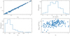 |
Fig. 1. General properties of the cluster sample used in this work (186 clusters). Upper left: X-ray redshift measured in this work compared to the optical redshift from the literature. Lower left: distribution of the redshift of the clusters in our sample. Upper right: distribution of the emission-weighted (spectroscopic-like) temperature in the radial range [0.1, 0.4]r500 across the sample. Lower right: distribution of M500, estimated according to Eq. (3), plotted versus redshift. |
The global temperature ⟨kT⟩ (or “spectroscopic-like” temperature, see Mazzotta et al. 2004) is measured by fitting the spectrum extracted in the region 0.1r500 < r < 0.4r500, a choice that is often adopted to obtain temperature values that more closely trace an ideal virial value, avoiding the effect of the cool core, when present. We use a single-temperature apec model, therefore ⟨kT⟩ is an emission-weighted value resulting from the range of temperatures present in the explored radial range. We find that the values of ⟨kT⟩ range from 4 to 12 keV, with a minority of clusters with ⟨kT⟩< 4 keV (see top-right panel of Fig. 1).
To estimate r500, we use the average relation described in Vikhlinin et al. (2006), which has been widely adopted in literature (Baldi et al. 2012; Liu et al. 2018; Mernier et al. 2019):
 (2)
(2)
where E(z) = (Ωm(1 + z)3 + ΩΛ)0.5. The global temperature ⟨kT⟩ and r500 are evaluated iteratively until converged. The total mass within r500 is also estimated from the scaling relation in Vikhlinin et al. (2006), or, equivalently, can be written as:
 (3)
(3)
where ρc(z) = 3H2(z)/8πG is the critical density at cluster’s redshift. Our sample spans a mass range of [1, 16] × 1014 M⊙, with only four clusters with M500 < 2 × 10¹⁴ M⊙ (see bottom-right panel of Fig. 1). We also note a posteriori that r500 is within the ACIS-I or ACIS-S1 field of view except for ten clusters, where the field of view covers only a radius of ∼0.6r500. In these cases, the ICM density profile up to r500 is obtained by extrapolating the profile beyond 0.6r500, an approximation that may not be extremely accurate but it may introduce only a few percent of uncertainty in less than 5% of our sample, which is well below the statistical errors.
Since cool-core and non-cool-core clusters are significantly different in both the abundance and spatial distribution of iron in the ICM, we estimate the fraction of cool-core clusters in our sample with the surface brightness concentration cSB (Santos et al. 2008, 2010), defined as the ratio of the fluxes observed within 40 kpc and 400 kpc:
 (4)
(4)
The fluxes in Eq. (4) are computed in the 0.5–2 keV band, and are estimated directly from the net count rate after considering the “beheading effect” due to the K-correction that depends on redshift and the minimum temperature observed in the core (see Santos et al. 2010, for more details). We remark that the concentration parameter is a simple and reliable parameter to classify the cool-core strength, which is, in reality, a definition that involve complex physics (Hudson et al. 2010). A bimodal distribution can be seen in the top panel of Fig. 2, which reflects the bimodality of cool-core and non-cool-core clusters as already investigated in other properties like pseudo-entropy (see Sanderson et al. 2009; Hudson et al. 2010, for example). Clearly, a more robust classification of cool-core and non-cool-core clusters should rely on more diagnostics, for example, central cooling time, temperature drop, etc. However, since this is not the main focus of this paper, we do not carry out any further analysis on the cool-core properties of the clusters but, rather, we investigate the global fraction of cool cores in our sample. Using cSB < 0.075 and cSB > 0.155 as the thresholds between non-cool-core and weak cool-core, and weak and strong cool-core clusters, respectively (see Santos et al. 2008), we find that 72 clusters in our sample are non-cool-core clusters, while 46 and 68 are weak- and strong-cool-core clusters. These numbers correspond to a percentage of 38.7%, 24.7%, and 36.6% of non-cool-core, weak-cool-core, and strong-cool-core clusters, respectively.
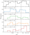 |
Fig. 2. Distribution of the surface brightness concentration cSB of the clusters in the full sample and in 4 independent redshift bins with roughly the same number of clusters (N). The vertical dashed lines indicate the threshold for non-cool-core and weak cool-core clusters: cSB = 0.075 and cSB = 0.155. |
Interestingly, the balance between cool-core and non-cool-core clusters in our sample is redshift-dependent. In the lower panels of Fig. 2, we show how the bimodality disappears at z > 0.2, while the cool-core clusters become dominant in the range z > 0.35. Given the coarse redshift binning, this is not in contradiction with previous claims on the dearth of cool-core clusters at z > 0.7 (see Santos et al. 2008), considering that we have only seven clusters at z > 0.7. In addition, we note that the requirement on the S/N slightly favors CC clusters as the redshift increases. Therefore, no claim can be made on the evolution of cool cores with cosmic time with the current sample.
Overall, assuming the fraction of ∼61% of clusters hosting a cool core in our sample is in line with what is usually found in X-ray selected samples, such as MACS, where Rossetti et al. (2017) found a cool-core fraction of (59 ± 5)%; however, it is significantly higher than the fraction found in SZ selected samples (∼30% for Planck clusters as found in Rossetti et al. 2017). This discrepancy, which is robust against differences in the detailed definition of cool-core, is the well known “cool core bias” (e.g., Eckert et al. 2011; Andrade-Santos et al. 2017) and may affect the overall thermal and chemical properties of a sample. In general, our sample shares the same core properties as other X-ray selected samples, despite its inclusion of a sizeable fraction of SZ-selected clusters.
3.2. Azimuthally-averaged profiles of electron density, iron abundance, and iron mass
We then measure the azimuthally-averaged profiles of gas density and iron abundance and, consequently, the iron mass cumulative profile. While accurate deprojection is always mandatory for density profiles, we chose to use only the projected profiles for iron abundance. The reason for this choice is twofold. First, since the typical metallicity variation across a cluster is usually smaller than a factor of ∼3 (∼Z⊙ at the iron peak to ∼Z⊙/3 in the outskirts), the projection effect has an actually mild impact on the measured abundance in most of the cases. Second, deprojection on metallicity usually requires much more photons but results in a much larger error in single measurement. If the cluster deviates from perfect spherical symmetry, which is, in fact, very common, deprojection induces extra uncertainty, which can not be properly assessed. It is for these reasons that we adopted deprojected profiles of density and projected profiles of iron abundance. This is a procedure that is commonly adopted in recent papers dealing with ICM abundance (see, e.g., Mernier et al. 2017; Lovisari & Reiprich 2019). The potential impact of this assumption is discussed in Sect. 4.
Each iron abundance profile contains six to 13 radial bins out to the extraction radius Rext ∼ 0.4r500, roughly corresponding to ∼0.25 r200. As previously discussed, this extraction radius is chosen on the basis of the expected iron plateau in most of the clusters, which is typically reached at these radii (see Urban et al. 2017). The inner and outer radii are adjusted to ensure that each bin encloses similar number of net photons. The minimum net photons in 0.5–7 keV energy band within each bin is 800 and can reach > 20 000 in some bright clusters with very deep observations. The spectrum of each bin is fitted with a double-vapec model, with independent temperatures and linked abundance, as described in Sect. 2.
Based on this modelization, we can efficiently remove the bias on the best-fit abundance value when the temperature gradient is significant within the spatial bin (see Molendi et al. 2016), especially in the center of cool-core clusters. In fact, in most cases we find no significant difference between the iron abundance obtained by fitting with a double vapec model and a single vapec or apec model. The use of double-temperature has little or no impact on metallicity outside the cool core. In spite of this, for the sake of simplicity, we do not change the spectral-fitting strategy with radius and we use a metallicity-linked double-vapec model to fit the spectral both within and outside the cool core. On the other hand, no attempt is made to consider different abundance values associated with different gas phases within a projected bin since it is not possible to investigate such an effect with present-day data. In fact, a relevant effect would be given by correlated fluctuations in the ICM density and abundance on a small (∼kpc) scale, an occurrence which has been never observed and is not expected. The only exception is given by the galactic coronae around BCGs (see Vikhlinin et al. 2001) and presence of low-surface brightness infalling clumps at large radii, which has been treated in dedicated works and is not expected to affect radii smaller than r500 (see Eckert et al. 2015). Therefore, we conclude that the assumption of a constant abundance in each projected bin is accurate for our science goals, and it provides a robust description of the actual azymuthally-averaged abundance profile.
The projected iron abundance profiles of all the clusters in our sample are plotted in Fig. 3, where the yellow points show the sample-average in seven radial bins. We confirm that, on average, the iron peak appears at radii < 0.1r500, while a plateau, or a very weakly decreasing profile, is evident at radii > 0.2r500.
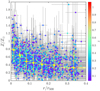 |
Fig. 3. Projected iron abundance profiles for all the clusters in our sample. Each point, color-coded by redshift, is the best-fit value in the corresponding radial bin. For clarity error bars are shown in light grey. The yellow points show the sample-average abundance and rms within seven radial bins. |
We fit the measured iron abundance profiles with a double-component model. The first component is a β model to fit the iron peak, while the second component is a constant representing the iron plateau:
![Mathematical equation: $$ \begin{aligned} Z = Z_{\rm peak}\cdot \left[1+\left(\frac{r}{r_0}\right)^2\right]^{-\alpha }+Z_{\rm plateau}. \end{aligned} $$](/articles/aa/full_html/2020/05/aa37506-20/aa37506-20-eq5.gif) (5)
(5)
The central drop component is not considered if not in the few cases where the innermost two-to-three bins are significantly lower than the outer bins. In this way we do not force this component to be used when the statistical significance is low. In fact, a systematic study of the iron drop is feasible only for nearby clusters (Liu et al. 2019), while a search throughout our sample would be dominated by noise. Despite this, the few cases where a central drop improves significantly the fit are discussed in Sect. 3.4.
For the electron density profiles, we extend the maximum extraction radius to ∼r500, and adopt a lower criterion of net photons in each bin in order to increase the spatial resolution. The spectrum in each bin is deprojected using the dsdeproj2 routine (Sanders & Fabian 2007; Russell et al. 2008), which deprojects a spectrum directly by subtracting the geometrically rescaled count rates of the foreground and background emission. The deprojected spectrum is then fitted with a single apec model. Electron density is derived directly from the geometrically scaled normalization parameter of the best-fit model:
![Mathematical equation: $$ \begin{aligned} \mathtt{norm} = \frac{10^{-14}}{4\pi [D_{\rm A}(1+z)]^2} \int n_{\rm e}n_{\rm p}\mathrm{d}V, \end{aligned} $$](/articles/aa/full_html/2020/05/aa37506-20/aa37506-20-eq6.gif) (6)
(6)
where z is the redshift of the cluster, DA is the corresponding angular diameter distance, V is the volume of the emission region. ne and np (nH) are the number densities of electron and proton. The ICM gas density is then computed by ρgas = nempA/Z, where mp is proton mass, A and Z are the average nuclear charge and mass of the ICM. For ICM with ∼1/3 solar abundance, A ≈ 1.4 and Z ≈ 1.2, and therefore ne ≈ 1.2np.
The deprojected electron density profiles are fitted with a double-β model, which can produce reasonable fit to the central density peak when a cool core is present. In the literature, the usual form of a double-β model used to describe density profiles, where density is computed from the surface brightness, is the square root of the quadratic sum of two β model components (e.g., Ettori 2000; Hudson et al. 2010; Ettori et al. 2013). Instead, the density in this work is measured directly from the deprojected spectrum, thus we simply adopt a double-β model as a linear summation of two β model components, that reads:
![Mathematical equation: $$ \begin{aligned} n_{\rm e}(r) = n_{01}\cdot \left[1+\left(\frac{r}{r_{01}}\right)^2\right]^{-3\beta _1 /2} + n_{02}\cdot \left[1+\left(\frac{r}{r_{02}}\right)^2\right]^{-3\beta _2 /2}. \end{aligned} $$](/articles/aa/full_html/2020/05/aa37506-20/aa37506-20-eq7.gif) (7)
(7)
For completeness, we also repeat the fit of the density profiles using the more conventional form of the quadratic sum of two β models, and find that the results are in very good agreement with those obtained using Eq. (7).
The best fits for the electron density profile ne(r) obtained with the double-β model are shown in the left panel of Fig. 4. From the iron abundance ![Mathematical equation: $ Z \equiv [n_{\mathrm{Fe}}/n_{\mathrm{H}}]/[n_{\mathrm{Fe}}^{\odot}/n_{\mathrm{H}}^{\odot}] $](/articles/aa/full_html/2020/05/aa37506-20/aa37506-20-eq8.gif) , assuming the same solar abundance used in the Xspec spectral fits
, assuming the same solar abundance used in the Xspec spectral fits ![Mathematical equation: $ [n_{\mathrm{Fe}}^{\odot}/n_{\mathrm{H}}^{\odot}] = 3.16\times 10^{-5} $](/articles/aa/full_html/2020/05/aa37506-20/aa37506-20-eq9.gif) (from Asplund et al. 2009), we then derive the cumulative profile of the Fe mass MFe(< r), as shown in the right panel of Fig. 4. We note that since our iron abundance profiles extend only up to 0.4r500, at larger radii, the iron mass is computed extrapolating the constant plateau up to r500, differently from the gas mass that is obtained from the data extending up to ∼r500. Therefore, the cumulative mass value above 0.4r500 depends on the assumption of a constant plateau at any radius. We note there that if the large scale iron distribution is, instead, a shallow power law, we may overestimate the total iron mass. Unfortunately, the measurement of the shape of the large scale iron profile (i.e., adopting a power-law instead of a constant plateau) across our sample is not within our reach. The assumption of a constant plateau is a clear limitation of our approach. A possible way out, but only for a minority of our sample, is to combine Chandra and XMM-Newton data, a strategy that is briefly mentioned in the discussion section of this paper.
(from Asplund et al. 2009), we then derive the cumulative profile of the Fe mass MFe(< r), as shown in the right panel of Fig. 4. We note that since our iron abundance profiles extend only up to 0.4r500, at larger radii, the iron mass is computed extrapolating the constant plateau up to r500, differently from the gas mass that is obtained from the data extending up to ∼r500. Therefore, the cumulative mass value above 0.4r500 depends on the assumption of a constant plateau at any radius. We note there that if the large scale iron distribution is, instead, a shallow power law, we may overestimate the total iron mass. Unfortunately, the measurement of the shape of the large scale iron profile (i.e., adopting a power-law instead of a constant plateau) across our sample is not within our reach. The assumption of a constant plateau is a clear limitation of our approach. A possible way out, but only for a minority of our sample, is to combine Chandra and XMM-Newton data, a strategy that is briefly mentioned in the discussion section of this paper.
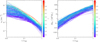 |
Fig. 4. Left panel: best-fit double-β model of the deprojected density profiles, color-coded by redshift, for all the clusters in our sample. Right panel: total iron mass profiles obtained by convolving the gas density profile with the best fit abundance profile for each cluster in our sample. At r > 0.4r500 the iron mass is computed extrapolating the constant plateau up to r500. |
3.3. The identification of two components in ZFe profiles
A necessary step before proceeding in our analysis is to check whether the use of a double-component model is statistically preferred to a simpler model. In other words, we want to assess the relevance of the two components not only on the basis of theoretical premises, but also from a blind fit of the measured abundance profiles. The relevance of this check is twofold. First, the distribution of iron in the ICM is sensitive to many dynamical processes, such as the outflow of central AGN, and large-scale sloshing. Some of these processes have relatively weak impact on the global morphology, but may significantly affect the distribution of iron. In these cases, the iron profile may not follow our idealized pattern of a central peak plus a constant plateau, even in the case of a rather regular morphology. Second, due to the relatively small extraction radii of the profiles (0.4r500), the iron plateau may not be well identified in cases where the iron peak has a large extension. Therefore, we repeat the fit of the iron abundance profiles, using a single-β model, without the iron plateau, and compare the goodness of the fit, estimated by the P-value of the two models. We note that a β model can provide an accurate description also in the case of a power-law behavior, which is typically obtained with small values for the core radius and the radial slope. Moreover, we are aware that the fit with a single-β model clearly predicts a rapidly declining metallicity value in the regions at radii > 0.4r500 not sampled by our data. This is in contradiction with the current and sparse knowledge about the ICM metallicity in the few clusters where outskirts have been properly studied (e.g., Urban et al. 2017; Mernier et al. 2018). As we have already stressed, we have no control on the actual abundance profile at large radii, so a constant plateau is one assumption of our modelization. In any case, the goal of this statistical test is to evaluate the robustness of our description on the basis of the data without using any prior.
We plot in Fig. 5 the (1 − P) value, which indicates the confidence level at which the fit is rejected. If we consider the 90% c.l. as our tolerance threshold, we find 16 clusters, shown as yellow circles in Fig. 5, for which both models are formally rejected. We check the images of the 16 clusters with these peculiar iron abundance profiles, and find no obvious signs of a disturbed morphology. Despite that, the iron profile appears to be dominated by significant intrinsic scatter between different annuli, making it impossible to fit the profile with a smoothly varying function. As we mentioned, there are various processes that can result in these peculiar profiles, for example, unnoticed mergers, major AGN outflows, core-sloshing in different scales, and projected gas clumps in cluster outskirts, among others. A concrete diagnosis on the physical reasons of the peculiar distribution of iron in these cases requires a more in-depth and case-by-case study of the dynamics of each cluster, which goes well beyond the goal of this paper. Therefore, we decide to exclude these 16 clusters in our following analysis and focus on a sample of the remaining 170 clusters.
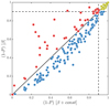 |
Fig. 5. Probability of rejection of the abundance profiles with and without the iron plateau. The dashed lines mark (1 − P) = 0.90, hence the yellow points shows clusters for which both the single- and double-component models are rejected at >90% c.l. Clusters colored in red favor the double-component model, while both models provide similar quality fits to the clusters colored in blue. In these cases, the double-component model returns a slightly lower goodness because of the inclusion of an additional parameter in the fit. |
In 39 clusters (colored in red), the double-component model provides a smaller (1 − P) value. Despite in several cases the difference is not dramatic, we find that at least in 1/5 of the sample the use of a double component in the iron distribution provides a significantly better fit, after considering the additional parameter. In the remaining 131 clusters, the profiles can be well fitted with both models within a confidence level of > 90%. In these cases, the double-component model returns a larger (1 − P) value because it has an additional free parameter and therefore a larger number of degrees of freedom.
One example for each of these three classes is shown in Fig. 6. The left panel shows a noisy iron abundance profile, that can be hardly reconciled with any smoothly-varying azimuthal function of the kind we consider here. In the central panel, the data clearly show a flat plateau that cannot be fitted with a single-β model. In some other cases, the central iron profile is better described by a broad bump rather than a well-defined peak, so that the plateau does not stand out clearly in the data. This situation is shown in the right panel, where it is not possible to differentiate statistically between the two models, and the abundance profile itself is indistinguishable from a simple power-law, at least in the explored range. For completeness, we repeat the same test, but using a power-law instead of a β model with no plateau. The results are very close to what we obtained in Fig. 5.
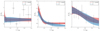 |
Fig. 6. Examples of abundance profiles with the corresponding double-component (red) and single-component (blue) best-fit models. From left to right: Abell 2050, CLJ1415+3612, and PSZ2 G241.77−24.00. The three examples are extracted from the yellow, red, and blue dots in Fig. 5, which are clusters that: cannot be fitted with either model (yellow); favor the double-component model (red); and can be fitted with both models in the observed radial range (blue). The best-fit values and uncertainties (of all the curve fittings in this paper, unless noted otherwise) are obtained using the MCMC tool of Foreman-Mackey et al. (2013). |
In general, we conclude that the β model with a constant plateau is statistically preferred with respect to the use of a single β model or power-law for a significant fraction of our sample. Clearly, a more complete modelling of the profiles would be a β model plus an transitional power-law, constrained to have a mild slope, plus a constant plateau in the external regions. A slow decrease is actually expected in some modelization of the iron distribution (see Mernier et al. 2017; Biffi et al. 2018b) and can be used to describe an intermediate regime where the iron distribution, far from the core, is still slowly decreasing before reaching the flat plateau associated to the pristine, uniform enrichment. However, the quality of data we use in this work is clearly not sufficient to assess the presence of this transitional component between the iron peak and plateau. We will dedicate a future work on a more extended modelization of the iron distribution, mostly in the perspective of the future X-ray missions (Tozzi et al., in prep.).
Finally, we also inspected the distribution of the size of the iron peak. Differently from what we have done in Liu et al. (2018), we can now directly compute an effective size of the iron peak as  , where r0 and α are the two best-fit parameters that fully characterize the shape of the peak. In principle, the global distribution of rFe reflects different physical phenomenon, including the effects of past or recent mergers that erased the peak or smoothed it into a broad bump, along with the broadening effects of the AGN feedback from the BCG plus minor mergers. In practice, it is impossible to disentangle the two phenomena. However, the broadening of the iron peak due to AGN feedback can be investigated by selecting the stronger cool cores, which are most likely to be the oldest ones, where no major merger had recently occurred. In this case, the typical size can be a way to parameterize the age of the peak through the broadening effect of the AGN feedback. This is what we have done in Liu et al. (2018) based on a sample with bright and strong cool core to reach the conclusion that the size of the iron peak of CC clusters is actually increasing by a factor of 3 with cosmic time in the redshift range 0.1 < z < 1. If we consider the CC clusters in our sample (defined as usual as those with cSB > 0.075), we find the same trend but weaker, consistent with the fact that, having a sample with less concentrated cores, we are including a wider range of ages for the observed iron peak, with younger peaks being narrower. The trend we obtain is an average increase of a factor of 2 (from 0.025 to 0.05r500) in the redshift range 0.05 < z < 0.6, still consistent with what we have found in Liu et al. (2018).
To summarize, we find that the choice to fit the abundance distribution with a β model along with a constant plateau is a good compromise between a comprehensive physical modelization and the data quality and that it is adequate to effectively describe a large sample of clusters observed with Chandra with a wide range in mass, redshift, and exposure time. While a two-component model is physically motivated and favoured by the data, a more sophisticated approach is not able to extract more information. Ideally, we should try to have more handle on the abundance profile at large radii. However, due to the limited field of view of ACIS, but mostly because of the rapidly decreasing signal, this is unfeasible. In fact, as we already mentioned, despite that the surface brightness is detected up to r500 in most of our clusters, at radii larger than 0.4r500, the spectral analysis would be strongly affected by uncertainties in the background subtraction. There are two ways to tackle this issue. The first is to use XMM-Newton for the clusters that have been observed with both instruments, exploiting the ∼5× larger collecting efficiency and the larger field of view. However, the discrepancy in the temperature measurements between Chandra and XMM-Newton (e.g., Schellenberger et al. 2015) increases the complexity of such a combined analysis. The second method is to wait for the X-ray micro-calorimeter Resolve onboard XRISM3, which is able to identify the iron line thanks to the ∼10× larger spectral resolution, in external regions of nearby clusters where angular resolution is not an issue; nonetheless, this would require a substantial investment of observing time due to the limited grasp of the bolometer. The first method goes beyond the goal of this paper and it is deferred to a further work on the entire Chandra and XMM-Newton archives. The second approach is definitely a time-consuming but promising way to use XRISM to tackle this problem (see Kitayama et al. 2014, for more XRISM science related to clusters), as we mention also in the discussion further on in this paper.
3.4. The effect of the central iron drop
The central iron drop observed in a few clusters is a significant feature with a typical scale of ∼10 kpc (Panagoulia et al. 2015; Liu et al. 2019; Lakhchaura et al. 2019). It requires a high spatial resolution and a high S/N to be detected and it has a negligible impact on the iron mass in most cases. We do not perform a systematic investigation of the iron drop in our sample due to the lack of a signal. Instead, we proceed by first identifying about 20 profiles that, following a visual inspection, may show a central drop. Typically, this occurs when the first or second bin shows an abundance value lower than the value of the second or third bin at ∼2σ. Then, we repeat the fit to the abundance profile including the central drop, allowing for this component in our fit in the form of a “negative Gaussian” as follows:
![Mathematical equation: $$ \begin{aligned} Z = Z_{\rm peak}\cdot \left[1+\left(\frac{r}{r_0}\right)^2\right]^{-\alpha }-a\cdot \mathrm{exp}\left[\frac{-(r-\mu )^{2}}{2\sigma ^2}\right]+Z_{\rm plateau}. \end{aligned} $$](/articles/aa/full_html/2020/05/aa37506-20/aa37506-20-eq11.gif) (8)
(8)
This modelization of the central drop is simpler than the one used in Liu et al. (2019) due to the lower quality of the profiles; it has also been used in Mernier et al. (2017). Then we collect all the cases where the improvement of the χ2 formally corresponds to a confidence level of 90%. In the end, we do find a central iron drop in eight out of 186 clusters. An example of this is shown in Fig. 7. The typical size of the iron drop measured in these eight clusters is ∼[0.05–0.1]r500, which is significantly larger than what has been found in nearby clusters and groups (Panagoulia et al. 2015; Liu et al. 2019). However, this is probably due to the relatively low resolution of the profiles we have in this work, which masks the small-scale iron drops, leaving only the large-scale ones. For these clusters, the final iron peak component is therefore computed by considering the “hole” in the iron distribution. Clearly, the amount of mass removed by the drop is limited to less than 10% of the total iron mass in the peak and it is often compensated by the re-adjustment of the iron peak profile, so that the impact on our final results is negligible. Nevertheless, we stress that the presence of a central drop in the iron distribution is an important component to be included when more detailed profiles are available, not only for its effect on the total iron budget, but also for its physical relevance. The effects of feedback and of dust depletion, which are responsible of the iron drop, are indeed expected to be present at least since z ∼ 1.
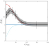 |
Fig. 7. Iron abundance profile of MACSJ0242.5−2132 with the best-fit showing a pronounced central iron drop. The red, cyan, and blue curves are the iron peak, iron drop, and iron plateau, respectively, as described by Eq. (8). |
3.5. Gas mass-weighted iron abundance
As already mentioned in Sect. 3.2, we first compute the average gas mass-weighted iron abundance, defined as  , without making any distinction between the two components. Here the index i runs over the annuli. In addition, where we are at radii r > 0.4r500, we simply have
  . Liu et al. (2018) have shown that gas mass-weighted value is more appropriate than the emission-weighted value in quantifying the average abundance of iron in the ICM because the latter, despite being much easier to measure4, can be affected by a significant bias in cool-core clusters. We note that the gas mass-weighted abundance is by definition different from a truly mass-weighted abundance as that obtained from numerical simulations, for instance. The point is that we assume a smooth ICM (i.e., not clumped) distribution within the angular scales resolved in the bins of our spectral analysis. Differently, in the presence of significant unresolved clumps, the emission-weighted value over-represents the cooler ICM. Therefore, excluding the presence of significant clumpiness, the observed gas mass can be considered an accurate estimate of the true gas mass, and the product of the emission-weighted abundance measured in each radial bin of the spectral analysis by the gas mass in that spherical shell can be considered a reliable proxy of the true gas mass-weighted abundance.
We show the gas mass-weighted iron abundance within r500 as a function of redshift in the left panel of Fig. 8. From a visual inspection, a good guess is to assume a value constant with redshift. If we compute the root mean square value around the mean over the redshift, or the raw scatter as defined in Pratt et al. (2009), we find that both quantities are comparable to the average statistical error. This implies that the intrinsic scatter, which is beyond any doubt present in a complex quantity such as Zmw(r < r500), is negligible with respect to the measurement uncertainty. Considering that the uncertainty on the redshift is not relevant here, we can safely search for a best-fit function by a simple χ2 minimization. If we fit the Zmw − z relation with a simple power-law defined as Zmw = Zmw, 0 ⋅ (1 + z)−γmw, we obtain the best-fit parameters Zmw, 0 = (0.38±0.03) Z⊙ and γmw = 0.28 ± 0.31, consistent with no evolution of Zmw across our sample.
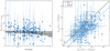 |
Fig. 8. Left panel: correlation between the average, gas mass-weighted iron abundance (within r500) and the redshift of all the clusters. The black curve and shaded area show the best-fit function Zmw = Zmw, 0 ⋅ (1 + z)−γmw with Zmw, 0 = (0.38 ± 0.03) Z⊙ and γmw = 0.28 ± 0.31. Right panel: gas mass-weighted abundance within 0.4r500 plotted against the emission-weighted value in the same radial range. The solid line corresponds to Zmw = Zew. Dashed lines show the average relation for cool-core and non-cool-core clusters, |
Limited by the extraction radius of our iron abundance profiles, the comparison between the gas mass- and emission-weighted abundances is only possible within 0.4r500. The last quantity is simply obtained fitting with a metallicity-linked double-temperature vapec model to the total emission within the same radius. In the right panel of Fig. 8 we compare the two quantities. We find that, on average, the emission-weighted abundance within 0.4r500 is higher than the gas mass-weighted value by ∼18%. We note that this is slightly lower than that found in Liu et al. (2018), where (Zew − Zmw)/Zmw ≈ 0.25. However, this is expected because most of the clusters in Liu et al. (2018) host a strong cool core, and the investigated radius is 0.2r500, thus, it is more affected by the iron peak. We expect that the difference between gas mass- and emission-weighted abundance would further decrease with larger extraction radius and higher fraction of non-cool-core clusters in the sample. This effect is more evident if we split our samples into two halves, populated by cool-core and non-cool-core clusters adopting as a threshold cSB = 0.075. We find that this discrepancy becomes 22% for cool-core clusters and drops to only 4% for non-cool-core clusters. A simple fit to the distribution with a linear function Zmw = Zew − δZ gives δZ = 0.11 Z⊙ for cool-core clusters, and δZ = 0.02 Z⊙ for non-cool-core clusters. The different behaviors of cool-core and non-cool-core clusters reflect the effect of the iron peak on the measurement of emission-weighted abundance.
The average emission-weighted abundance within 0.4r500 of cool-core clusters in our sample is (0.51 ± 0.01) Z⊙, significantly higher than that of non-cool-core clusters: (0.41 ± 0.01) Z⊙. This difference has been already noticed in several other works (e.g., De Grandi & Molendi 2001; De Grandi et al. 2004). We find that this difference is significantly reduced albeit still marginally significant when considering the average gas mass-weighted abundance, which turns out to be (0.41 ± 0.01) Z⊙ and (0.38 ± 0.02) Z⊙ for cool-core and non-cool-core clusters, respectively. These results confirm that the difference in iron abundance between cool-core and non-cool-core clusters is largely due to the use of emission-weighted abundance, while it almost disappears when using gas mass-weighted values, which are representative of the true iron mass content. At the same time, a residual difference in the average, gas mass-weighted abundances shows that the effect is not entirely due to the different ICM distribution, but it may be due to a slightly larger amount of iron in cool-core clusters, further strengthening the hypothesis of two different physical origins for the iron peak and the iron plateau.
3.6. The properties of the iron plateau and iron peak
In this section, we analyze the profiles of iron abundance and iron mass by resolving the two components, namely the iron plateau and the iron peak. From Fig. 9, we can immediately assess the contributions of the two components to the iron mass budget. In Fig. 10, we show the distribution of the ratio of iron peak mass to iron plateau mass within r500, and also the correlation of the ratio with redshift. No redshift-dependence of the ratio is found based on Fig. 10. Despite that the ratios for most clusters are distributed within the range of [5 × 10⁻⁵, 0.5] and centered at 0.008, we find clusters with extremely low iron peak mass. We check the spectral fits and profile fits for these cases and find that the clusters with low iron peak mass are consistently non-cool-core clusters which host no iron peak or a very weak iron peak in the center. A small number of clusters show  ; in these cases, the central iron distribution is broad and slowly declining, so that it is ascribed mostly to the central peak. These cases would probably be better described by a third component in the form of a shallow power-law, however, the quality of the data makes it impossible to identify such additional component. In these cases, the iron mass in the peak should not be associated to the BCG but, rather, to the mix of the two components that appears as a broad bump. This is admittedly a limitation of the method since it is impossible to spatially separate the two components when the central peak has been smeared out.
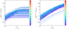 |
Fig. 9. Left panel: cumulative iron mass profiles corresponding to the peak component, color-coded by redshift for all the 170 clusters with regular abundance profiles considered in this work. Right panel: as in the left panel, but for the plateau component. |
We also note, based on Fig. 10 and also the right panel of Fig. 9, that a few clusters have a very low iron plateau. We check the profiles of these clusters, and find that this is mostly driven from one or more measurements of very low abundance in the outskirts, probably due to the low S/N of the data. A bias toward low abundance values in the outer regions has been noticed, and it has been shown that it can be removed by excluding the 0.9–1.3 keV rest-frame band (corresponding to the iron L band emission complex, S. Molendi, priv. comm.). However, due to the limited signal of the spectra in the outer bins, we are not able to verify this effect nor the robustness of these low measurements. If, in these cases, we fix the iron plateau to some value, for example, 0.2 Z⊙, we find that the ratio between the iron peak and iron plateau becomes, by construction, consistent with the average value of the sample, while the fit to the profiles are still good due to the poor statistical weight of the low-abundance data points in outskirts. This, in fact, implies that we have a very loose constraint on the iron plateau in several clusters, which is, nevertheless, already accounted for in the uncertainty of the fitting result. Given the low number of clusters with Zplateau ∼ 0 (5 out of 170), these cases do not require a change of our fitting strategy nor have an impact on our final results.
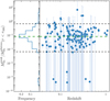 |
Fig. 10. Distribution of the ratio of iron peak mass to iron plateau mass within r500, and the correlation with redshift. The green dashed line indicates the weighted average at ∼0.008. The black dashed lines mark the [5 × 10⁻⁵, 0.5] range roughly corresponding to >90% of the clusters symmetrically distributed around the central value (as shown in the left-side panel). |
We then check the normalization of the iron plateau (Zplateau) across the sample. In the upper panels of Fig. 11, we present the distribution of Zplateau and its relation with redshift. From the upper left panel of Fig. 11, we can immediately observe that the distribution of Zplateau fits a symmetrical Gaussian well. This implies that the plateau is made up of many additive processes all acting independently, which is quite consistent with the picture that a wide range of randomly sampled galaxies eject out metals that are all adding up in the plateau ICM. We compute the weighted average of Zplateau (where the weights are defined  ) and find ⟨Zplateau⟩ = 0.38 Z⊙, thus consistent with a 1/3 solar abundance of the ICM in cluster outskirts, a value that has been commonly reported by many works (see Serlemitsos et al. 1977; Mushotzky et al. 1996; Simionescu et al. 2013; Molendi et al. 2016; Urban et al. 2017, for example). The arithmetic mean is also ⟨Zplateau⟩ = 0.38 Z⊙, while the total scatter with respect to the mean is 0.14 Z⊙. Since the average statistical error is 0.11 Z⊙, we can estimate the intrinsic scatter assuming
  , obtaining σintr = 0.09 Z⊙. The intrinsic scatter of the plateau normalization, therefore, is lower but not negligible with respect to the statistical uncertainty. This is shown in the upper-left panel of Fig. 11, where the histogram of the best-fit values of Zplateau is shown with a Gaussian centered on ⟨Zplateau⟩ and with width equal to the average statistical error. This implies that the intrinsic fluctuations in the plateau, which are naturally expected, amount to ∼25% of the average plateau value. This is consistent with a roughly uniform enrichment at high-z at least in the massive cluster range.
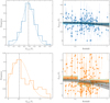 |
Fig. 11. Upper left: distribution of the abundance of the iron plateau component Zplateau. The dashed line indicates the weighted average value ⟨Zplateau⟩ = 0.38 Z⊙. The dashed curve shows a normalized Gaussian with σ = 0.11 Z⊙, corresponding to the average statistical error, and μ = 0.38 Z⊙, corresponding to the weighted average value. Upper right: abundance of the iron plateau plotted against cluster redshift. The black curve and shaded area show the best-fit function Zplateau = Zplateau, 0 ⋅ (1 + z)−γplateau with Zplateau, 0 = (0.41 ± 0.02) Z⊙ and γplateau = 0.21 ± 0.18, which are obtained by fitting the weighted average values and uncertainties of the four bins shown as blue solid lines and shaded areas. Lower left: distribution of the normalization of the iron peak component Zpeak. The dashed line indicates the weighted average value ⟨Zpeak⟩ = 0.52 Z⊙. The dashed curve shows a normalized Gaussian with σ = 0.42 Z⊙, corresponding to the average statistical error, and μ = 0.52 Z⊙, corresponding to the weighted average value. Lower right: normalization of the iron peak component Zpeak plotted against cluster redshift. The black curve and shaded area show the best-fit function Zpeak = Zpeak, 0 ⋅ (1 + z)−γpeak with Zpeak, 0 = (0.68 ± 0.07) Z⊙ and γpeak = 0.79 ± 0.53. |
These results hold under the assumption of a constant plateau normalization as a function of redshift. If we then focus on the evolution, from the top-right panel of Fig. 11, we can immediately notice the absence of a significant correlation with redshift.
Given the presence of a significant scatter in Zplateau, we should not fit the Zplateau − z relation with a simple χ2 minimization. To describe the properties of the iron plateau as a function of redshift, we decide to focus on four bins of redshift with a similar number of clusters, namely z < 0.12, 0.12 < z < 0.2, 0.2 < z < 0.3, and z > 0.3, with about 42 points each. We inspect the histogram distribution of the Zplateau values in each redshift bin, and verify that the weighted mean ⟨Zplateau, z⟩ closely traces the peak of the distribution. Then, we are allowed to use a χ2 minimization on the four bins to fit the behavior of the Zplateau distribution with redshift. We adopt an empirical function Zplateau = Zplateau, 0 ⋅ (1 + z)−γplateau, and obtain Zplateau, 0 = (0.41 ± 0.02) Z⊙ and γplateau = 0.21 ± 0.18, suggesting no evolution with redshift. This corroborates the hypothesis that the plateau is dominated by the contribution from a pristine and uniform enrichment, which possibly occurred before the virialization of the main halo.
Then we focus on the normalization of the iron peak Zpeak. In the lower panels of Fig. 11, we show the statistic of Zpeak and the Zpeak − z distribution. Unlike the Zplateau, whose distribution is well approximated by a Gaussian, the distribution of Zpeak is closer to a power law, suggesting that the underlying process may be described by random jumps, such as intense star-formation events associated to intermittent cooling flows and responsible for the creation and ejection of metals. The weighted average value of Zpeak is ⟨Zpeak⟩ = 0.52 Z⊙, with a rms dispersion of 0.49 Z⊙. Since the average statistical error is 0.42 Z⊙, the estimated intrinsic (and symmetric) scatter is ∼0.26 Z⊙. This is clearly seen in the bottom-left panel of Fig. 11, where the Gaussian centered on the weighted mean and representing the width of the statistical uncertainties, fails in describing the right side of the distribution. The reason is that the high-Zpeak values represent a population of clusters which experienced a relatively low number of minor and major mergers, so that the central regions evolved undisturbed for several Gyr with the late, BCG-related iron piling-up in the core. Ideally, all massive clusters should show a high iron peak if the mass growth is smooth, but in reality, the stochastic merger events reset the thermodynamic and chemical properties of the cores, creating the distribution of properties that we actually observe.
The estimate of the intrinsic scatter is based on a double assumption: a symmetric intrinsic scatter, and a constant ⟨Zpeak⟩ value with redshift. We can immediately see from Fig. 11 that the first assumption is not met. To test the evolution of ⟨Zpeak⟩, we use a χ2 minimization on the four redshift bins as in the previous case. Using the same empirical function for Zplateau, we obtain Zpeak, 0 = (0.68 ± 0.07) Z⊙ and γpeak = 0.79 ± 0.53. This result, despite the large scatter of Zpeak across the sample, is consistent with an increase of ∼75% from z ∼ 1 to low-redshift, but it is also consistent with no evolution within less then 2σ. Also, we need to bear in mind that despite our sample spans a redshift range 0.04 < z < 1.1, the weight of high-z (z > 0.6) clusters is limited and the fit shown in the lower-right panel of Fig. 11 is actually driven by the data points at redshifts below 0.6. In any case, a mild, positive evolution with cosmic time, if confirmed, supports a different origin of the iron peak, more recent in time and associated with the central BCG and epochs after the cluster virialization (z < 1). In other words, the observed iron peaks are consistent with being formed within the cluster in situ around the BCG, increasing in strength from redshift ∼1 to local as the feedback cycle associated to the BCG creates short but intense period of star formations, with the associated creation and diffusion of iron. Considering the redshift distribution of our sample, this evolution, if any, is occurring on a time scale of about 5 Gyr, which corresponds to the interval: 0.05 < z < 0.6.
Finally, we explore the evolution of iron in terms of the iron mass of the two components. In Fig. 12, we plot this two components within r500 divided by the gas mass within the same radius against cluster redshift. We find that Mplateau/Mgas appears to be distributed around an average value with a scatter entirely consistent with the statistical uncertainty, and, therefore, we can investigate its redshift dependence directly with a χ2 minimization. On the contrary, the quantity Mpeak/Mgas shows a significant intrinsic scatter, and we adopt the same strategy as before, consisting in fitting the weighted mean ⟨Mpeak⟩ in four redshift bins. Using the same function X = n ⋅ (1 + z)−γ, we obtain  for the iron plateau, and
  for the iron peak. Therefore, we can confirm that the plateau does not seem to evolve significantly in this redshift range, which is consistent with an early (z > 2) and uniform enrichment. On the other hand, the iron peak mass shows some hint of an increase with cosmic time. This growth is not statistically significant, similarly to that observed in the peak normalization. If confirmed, we can interpret this trend, regardless of its large uncertainty, large scatter, and the incompleteness of our sample particularly at high-z, as an average increase of ∼100% of the amount of iron produced and/or released within the clusters in the central region at z < 1.
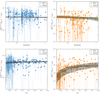 |
Fig. 12. Upper panels: ratio of iron mass of the plateau (left) and the peak (right) to the gas mass within r500 versus cluster redshift. The black curves show the best-fit functions |


The relatively recent origin of the iron peak and its strong dependence on the intermittent star formation history in the BCG, coupled to the stochastic merger events, are corroborated by the large observed scatter, particularly if compared to the scatter of the plateau. For the iron plateau mass (divided by gas mass), the total scatter turns out to be ∼90% of the average measurement (1σ) uncertainty, therefore implying no intrinsic scatter. Once again, this suggests an early and uniform enrichment. On the other hand, the distribution of the iron peak mass has a scatter several times higher than the statistical uncertainty: σtot ∼ 6 × σstat. This fact is due not only to a large diversity in the history of star formation episodes in the BCG responsible for the iron mass excess, abut also to the widely distributed dynamical age of the core, which strongly affects the ICM mass associated with the peak and, therefore, strongly amplifies the scatter with respect to the Zpeak distribution.
We know that the fraction of mass included in the iron peak is only ∼1% of the total iron mass in the ICM within r500. Therefore, the evolution of iron in the ICM is dominated by the amplitude of the iron plateau. The lack of evolution in the iron plateau, therefore, drives the total (peak plus plateau) iron abundance to be almost constant with redshift, as we already show in Fig. 8. Our approach also demonstrates that considering only the global abundance is not adequate to properly constrain the evolution and the physical origin of the (at least) two different components of the iron distribution.
We also investigate the possible difference in the behaviors of cool-core (cSB ≥ 0.075) and non-cool-core (cSB < 0.075) clusters. As can be seen in the top left panel of Fig. 12, cool-core and non-cool-core clusters do not show a different behavior when considering the iron plateau. However, we find from the upper right panel of Fig. 12 the expected result that non-cool-core clusters tend to be lower than cool-core clusters in the iron peak mass. To further explore the link between the iron peak and the presence of a cool core, we also investigate the correlation between the iron to gas mass ratios in the two components with the surface brightness concentration cSB, as shown in the lower panels of Fig. 12. We fit the distribution with a simple power-law, MFe/Mgas = A ⋅ (cSB)B. For the iron plateau, we obtain A = (5.7 ± 0.4)×10−4 and B = 0.05 ± 0.03. As expected, the strength of the cool core does not affect much the properties of the iron distribution on large scales. For the iron peak, we again divide the sample into four bins as before: cSB < 0.05, 0.05 < cSB < 0.095, 0.095 < cSB < 0.19, and cSB > 0.19, and fit the weighted average of the four bins. We obtain A = (5.4 ± 3.0)×10−5 and B = 1.32 ± 0.33, which implies a significant correlation between the amount of iron in the peak and the strength of the cool core. This is largely expected since the presence of a peak in the iron distribution has been always observed in association with a strongly peaked surface brightness, as already mentioned (De Grandi et al. 2004). Another way to express this result is in terms of the correlation of metallicity and density (or anticorrelation of metallicity and entropy) observed in the cluster center. This result is in line with the general picture that the iron peak is associated with the formation and evolution of the cool core, and it is mainly created in situ thanks to the periodic starburst occurring in the BCG. Here, a still missing link is the connection of the total amount of iron in the peak with the integrated star formation history consistent with the old stellar population of BCG. It is well known that episodic and recurrent starbursts occur in BCG, however a quantitative assessment of the amount of freshly (z < 1) produced iron in the BCG has never been accurately measured. The connection between the BCG star formation history and the iron peak will be investigated in a forthcoming paper (Liu et al., in prep.).
3.7. The correlation between M500 and iron abundance
In Fig. 13, we explore the relation between the gas mass-weighted abundance within r500 and M500, the total mass of the cluster within r500. As usual, we use a simple power-law Zmw = Z0 ⋅ (M500/1014 M⊙)−α. We perform a linear regression for the log(Z)−log(M) relation requiring a minimization of the orthogonal distance of the points from the best-fit relation, thus considering uncertainties in both quantities. The best-fit gives Z0 = (0.52 ± 0.08) Z⊙ and α = 0.14 ± 0.09. This implies that in the mass range [3–10] × 1014 M⊙, the global gas mass-weighted abundance change only by less than 20%, which is slightly higher at lower halo masses. Given the small mass range probed here, this is comparable to the correlation of stellar mass with halo mass found by Lin et al. (2012). Taken at face value, this relation would imply a rapidly increasing average abundance at lower masses (below 2 × 10¹⁴ M⊙ into the group regime), a range which is not explored here, based on the assumption that the entire stellar-mass budget is contributing to the chemical enrichment of the ICM. We must bear in mind, however, that Lin et al. (2012) do not include the contribution of the intracluster light (see Presotto et al. 2014, and references therein), that can be larger at high masses, effectively flattening the stellar mass – halo mass relation.
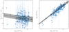 |
Fig. 13. Left: correlation between gas mass-weighted abundance within r500 and the total mass M500 for all the clusters in the sample. The black curve and shaded area denote the best fit function and the 1σ confidence interval: Zmw = (0.52 ± 0.08)⋅(M500/1014 M⊙)−0.14 ± 0.09. Right: correlation between the gas mass and M500. The black curve and shaded area denote the best fit function and the 1σ confidence interval: Mgas/1014 M⊙ = (0.131 ± 0.012)⋅(M500/1014 M⊙)1.05 ± 0.06. |
In the right panel of Fig. 13 we also show the correlation between the gas mass (within r500) and the total mass M500. Also in this case the statistical errors in both quantities are considered. The best-fit function of Mgas/1014 M⊙ = A ⋅ (M500/1014 M⊙)B gives A = 0.131 ± 0.012 and B = 1.05 ± 0.06. The slope we find here is still consistent with the value of 1.13 ± 0.03 found by Lin et al. (2012), which implied that smaller mass halos have slightly less ICM within r500 compared to the most massive clusters. However, despite the agreement, we do not find statistically significant evidence for this trend in our sample. If we include also a dependence on redshift of the form (1 + z)γ3 we find A = 0.130 ± 0.010, B = 1.04 ± 0.06 and γ3 = 0.08 ± 0.21, again in good agreement with Lin et al. (2012) and with previous claims by Vikhlinin et al. (2009). However, we remark that the observed evolution of fICM depends on cosmology (see Allen et al. 2011) and, therefore, we do not discuss possible physical implications for the trend found here.
A comprehensive discussion on the correlations between the integrated quantities (global metallicity, temperature, mass) has been postponed for the purposes of a forthcoming work.
4. Discussion
In this section, we discuss several aspects that range from the control of the systematics in our spectral analysis5 to the physical interpretation of our results and a direct comparison with previous works. We start from this last aspect, which is relevant here since the original motivation of this work was the contradictory results obtained in the last 10 years on the iron evolution in the ICM.
4.1. Comparison with previous works
Since the beginning of the era of Chandra and XMM, a number of attempts have been made to explore the cosmic evolution of ICM metal abundance. Although early works such as Tozzi et al. (2003) and Balestra et al. (2007) are likely to suffer from the limited size of cluster sample and the low S/N of the data, more recent works based on large samples and deeper observations present contradictory results and no obvious solution could be found to explain the observed discrepancies. Both the selection of the sample and the extraction radius used to measure the ICM abundance vary in these works, which increases the difficulty in comparing the previous results. Another issue is that all these previous results are obtained from emission-weighted measurements and, thus, they might be influenced by the fraction of cool-core clusters in the sample. This effect, as we know, would be mitigated, if not eliminated, once the gas mass-weighted abundances were used. Given these caveats, for the sake of comparison with the literature we consider only the evolution measurements based on the core-excised clusters, namely, using a radial range of 0.1 (or 0.15)−1r500. The functional form Z ∝ (1 + z)−γ is commonly used to quantify the evolution, thus, we can directly compare the slope γ. We list the measurements of γ in different works in Table 1, and compare them to the result we obtained by fitting the distribution of the gas mass-weighted abundance within r500 in this work.
Slope of the relation between average abundance and redshift from the literature compared to the values found in this work.
In general, we find that our results for the evolution of the gas mass-weighted abundance (γ = 0.28 ± 0.31) are consistent with most of the previous literature, based on emission-weighted measurements, with some noticeable exceptions. We first consider the results of Ettori et al. (2015), where significant and strong evolution is found in the innermost regions r < 0.1r500, whereas weaker and much less significant evolution is found at larger radii. While the evolution at small radii may be reconciled with our ∼2σ evolution in the peak component, we reconsider their results and average the [0.15–0.4]r500 and > 0.4r500 bins, finding γ = 0.48 ± 0.34, which is now consistent with our results. We also compare with the results of McDonald et al. (2016), where γ = 0.03 ± 0.06 for [0.15–1]r500, with a ∼2σ evolution when considering the full [0–1]r500 range. Again, given the expected effects of the emission-weighted analysis, we are fairly consistent with their results.
More difficult to reconcile are the results by Mantz et al. (2017), where no evolution is found in the very [0–0.1] and in the [0.5–1]r500 radial range, while a mild but very significant evolution is found for the range [0.1–0.5]r500. If we try to average their [0.1–0.5]r500 and [0.5–1]r500 bins, however, we find γ = 0.51 ± 0.46 which is again consistent with our findings. The point here is that a spatially-resolved analysis focusing on fixed radial bins normalized to r500 may not be adequate to properly follow the different components, so that the evolutionary behavior for fixed radial bins may return unstable results, unless the size and shape of each different component is properly identified.
Finally, the most discrepant result with respect to our findings is Maughan et al. (2008), where γ = 1.63 ± 0.35 is obtained based on a sample of 111 clusters6, suggesting a strong evolution at > 4σ c.l. However, we notice that a number of high-redshift clusters in the sample of Maughan et al. (2008) have only upper limits for the measured abundance, often with small uncertainties. This is probably due to the low S/N of the data. For example, Maughan et al. (2008) report an abundance  (adopting the solar abundance of Asplund et al. 2009) for CLJ1415.1+3612 at redshift 1. However, recent studies using deeper observations have presented much higher abundance of this cluster. For example, Santos et al. (2012) present a result of Z = 0.88 ± 0.11 within ∼0.35r500 (see also De Grandi et al. 2014), and in this work we consistently measure Z = 0.76 ± 0.12 within 0.4r500. If we remove this single data point, the best-fit slope decreases immediately from 1.63 ± 0.35 to 0.76 ± 0.35. Therefore, we suppose that the evolutionary signal detected by Maughan et al. (2008) is likely to be caused, at least partially, by several low S/N clusters at high redshifts which return unreliable low values of metallicity.
Moreover, we also explore the impact of the use of emission-weighted abundance on the evolutionary signal found in Maughan et al. (2008). Among the 115 clusters in the sample of Maughan et al. (2008), 48 are also in our sample. We therefore make a comparison between the gas mass-weighted abundance measured in this work, and the emission-weighted value provided in Maughan et al. (2008), as shown in Fig. 14. As expected, no significance evolution is found in the gas mass-weighted abundance, with γ = 0.25 ± 0.28, in perfect agreement with the full sample. On the other hand, for the emission-weighted abundance we obtain a best-fit γ of 0.95 ± 0.39. This result indicates that the use of emission-weighted abundance also contributes to the claim of evolution previously reported. In conclusion, past claims of evolution (or no evolution) are most likely due to the combined effect of the use of different sample selections (mostly X-ray versus SZ selected samples with different cool-core fractions) and emission-weighted abundance values, with the latter amplifying the effect of sample selection, especially in small samples. The use of larger samples, with a mixed selection function, and of gas mass-weighted measurements, shows a small amount of evolution within r500, if any, which is, according to our results, limited to the iron peak.
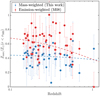 |
Fig. 14. Comparison between the gas mass-weighted abundance measured in this work and the emission-weighted abundance provided by Maughan et al. (2008), for the overlapping 48 clusters. The reference solar abundance for the data points of Maughan et al. (2008) has been adjusted from Anders & Grevesse (1989) to Asplund et al. (2009), for a direct comparison with our results. |
4.2. Projection effects
In this section, we estimate the impact of projection effect on the iron abundance profiles and, consequently, the final results. We repeat our analysis in a fraction (about 10%) of our sample, including clusters with the steepest abundance gradient to maximize the effects of projection. We find that, as expected, the plateau is almost unaffected by deprojection. Instead, the deprojected peak values are found, in a few cases, 10–20% higher than the projected ones. In particular, the normalization of the deprojected abundance in the iron peak is about 10–20% larger than the projected values and a larger effect, up to a maximum of ∼40%, is found for the deprojected iron peak mass. This is because a small change in the extension of the peak component is amplified by the volume effect.
We show the case of Abell 383, which hosts a strong cool core, a steep iron peak, and an intermediate S/N; therefore, it suffers a strongest projection effects among the clusters in our sample. The projected and deprojected abundance profiles of Abell 383 and the best-fit models are shown in Fig. 15. We find that the deprojection of the profile only induces a negligible change on the iron plateau. The main reason for this is that the plateau is dominated by the outer regions, where the projection effects are weak if not absent due to the flat temperature profile. Therefore, since the mass of the iron plateau contributes > 95% of the total iron mass budget, the impact of the projection effect on the total iron mass and the gas mass-weighted iron abundance within r500, is also negligible.
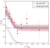 |
Fig. 15. Projected and deprojected iron abundance profiles of Abell 383: an example to show the impact of projection effect. The iron peak and iron plateau components in the best-fit model are plotted with dash-dotted lines and dashed lines, respectively. |
Instead, the iron peak is somewhat amplified by deprojection. In the case of Abell 383, the differences in the total iron mass, the iron plateau mass, and the gas mass-weighted abundance within r500 between projected and deprojected values are all lower than 3%. On the other hand, the normalization of the iron peak measured from the deprojected profile is 0.59 ± 0.21, ∼18% higher than that measured from the projected profile 0.50 ± 0.14. The deprojected iron peak mass within r500 is ∼43% higher than the projected value, since the slightly larger extension of the peak are amplified by the volume weighting. This increase, however, is smaller than the 1σ statistical errors, which, averaged over all the clusters in our sample, are equal to 48% and 67% for the normalization of the iron peak and the iron peak mass within r500, respectively. Since Abell 383 hosts one of the strongest iron peaks in our sample, these results can be taken conservatively as an upper limit of the magnitude of projection effect.
In summary, we acknowledge the fact that the strongest iron peaks in our analysis may be biased towards lower values by ∼few × 10%, mostly because of the uncertainty in the extension of the iron peak, which is a key quantity in determining Mpeak. We are also aware that any unnoticed irregular morphology in the central region may alter the deprojection results, which are based on a perfect spherical asymmetry and, even in the absence of such features, it is prone to amplification of noise. In other words, by applying deprojection, we risk introducing large random uncertainties possibly larger than the bias we aim to correct. Clearly, an accurate and stable quantification of the projection effect is possible only by taking into account many aspects, including the 3D morphology of the cluster emission and the 3D distributions of temperature and iron abundance, which is far beyond the goal of this paper, as well as the current state of advancement with regard to the technology that is available. Therefore, we decided to ignore the deprojection correction in this work and to present results based on the projected values of iron abundance.
4.3. The impact of nH on the measurement of iron abundance
The HI column density which quantifies the absorption of X-rays is an important factor that affects the fitting of X-ray spectra, in particular, the thermal continuum, therefore, also affecting the measurement of ICM metallicity. Usually there are three strategies to set the value of nH: (i) nH, LAB, the measurement from the Leiden/Argentine/Bonn (LAB) survey (Kalberla et al. 2005), which only takes into account the neutral hydrogen; (ii) nH, tot from Willingale et al. (2013), which also calculates the contribution of molecular and ionized hydrogen; (iii) nH, free, obtained directly by fitting the X-ray spectrum with nH set as a free parameter. The impact of these different values of nH on the measurement of metal abundance has been discussed in detail in Lovisari & Reiprich (2019). In general, nH, tot provides a better fit to the spectrum than nH, LAB. However, Lovisari & Reiprich (2019) also find that in a few cases, using nH, tot may not always be accurate. A safer strategy is obtained by setting nH free and putting some constraint on the range of possible values to avoid strong degeneracies with other parameters. This allows us to identify the preferred nH value without being too far from the reference value nH, tot. However, a caveat here is that the time-dependent contamination corrections of ACIS at low energies (below 2 keV) introduces some uncertainties in the Chandra calibration and this may also bias the measurement of nH. Therefore, we stress that leaving nH free and setting a constraint according to nH, tot, despite being an already very conservative strategy, does not always guarantee a return to the correct value for nH. In this framework, we adopt a two-step strategy: we fit the spectrum of the global emission by setting nH free to vary below a very loose upper limit at 10 × nH, tot, and obtain the nH, free; then for the spatially-resolved analysis, we adopt the measured nH, free, and allow it to vary within its statistical confidence interval, or within ±50% when its uncertainty is too small. With this strategy, we take into account not only the possible discrepancy between nH, tot and nH, free, but also the fluctuation of nH within the field of view of the cluster. We show in the upper panel of Fig. 16, the comparison between nH, tot and nH, free. Similarly to the result of Lovisari & Reiprich (2019), we find a general agreement between nH, tot and nH, free above 0.05 × 1022 cm−2, while the discrepancy is relatively large for low column densities, in which the best-fit values are systematically larger than nH, tot, despite being consistent within 1σ. In the lower panel of Fig. 16, we plot the ratios of all the abundance measured by adopting our strategy in nH (free to vary in a limited interval around nH, free) and by fixing nH to nH, tot, as a function of nH, tot. We only find a slight bias of few percent, Z/Z(nH, tot)∼0.98, with no dependence on nH, tot. Despite it being hard to decide whether nH, free or nH, tot is better for describing the absorption effects of the HI Galactic column density, we conclude that any effect related to nH is under control and it does not bias our results.
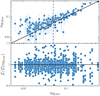 |
Fig. 16. Upper panel: comparison of the measured nH, free and nH, tot. The nH values are in units of 1022 cm−2. The vertical dashed line denotes 0.05 × 1022 cm−2. The solid line corresponds to nH, free = nH, tot. Lower panel: ratio of all the best-fit abundance values obtained by adopting our strategy in nH (free to vary in a limited interval around nH, free) and by fixing nH to nH, tot, as a function of nH, tot. |
4.4. Physical interpretation of the results and future perspectives
Our results are in general agreement with the well established picture that the bulk of iron in the ICM is produced at early epochs, approximately at z > 2, well before cluster virialization (see Willis et al. 2020). On the other hand, the signal of evolution of the iron peak, despite it being statistically weak, shows the complex effects of more recent processes occurring after cluster virialization (roughly z < 1), including the star formation and supernova explosion in member galaxies, the galaxy-scale dynamical activities which eject metals from the galaxies to the ICM, and the ICM motions induced by AGN feedback activities that continuously transport the metals from the cluster center to the outer regions. In particular, in Liu et al. (2018) we have shown the spatial broadening of the iron peak in a sample of 41 most relaxed Chandra clusters. However, in order to measure the size of the iron peak accurately, the sample in Liu et al. (2018) was selected with a strict requirement on cluster relaxation and we were not able to obtain any significant constraint on the evolution of the iron peak in mass. In this work, using a sample that is > 4 times larger, we find weak evidence for the evolution of the normalized mass content iron peak. We stress, however, that both the samples of Liu et al. (2018) and this work suffer from a not-well-defined selection in the total cluster mass. A coherent evolutionary picture of iron in the ICM will be reached only with a complete and large sample of galaxy clusters.
At present, the best sample is provided by the combination of the Chandra and XMM-Newton archives. Depending on the mass selection that can be adopted, the total number of clusters may reach ∼1000. Clearly, a proper spatially resolved analysis is feasible only for about 1/3 of the sample, while most of the clusters could be characterized by the X-ray morphology, a single temperature, and a single, average abundance. The abundance measurement would be emission-weighted, unless some priors on the abundance profile are assumed, to be combined with the observed surface brightness profile. In practice, the application of what we have learned with this sample to the largest sample that can be assembled today, would provide us with the most comprehensive study on ICM chemical evolution. Clearly, the ultimate test on the robustness of this approach would be available only when a mission like Athena (e.g., Barret et al. 2020), Lynx (Vikhlinin 2019) or AXIS (Mushotzky et al. 2019) would provide access to a large number of well-characterized, spatially resolved clusters with a wide range of halo mass and redshift. In particular, we stress the importance of keeping in line with a Chandra-like resolution, which is the only means with which we may sample the X-ray emission at scales below 10 kpc at any redshift, a mandatory requirement for any proper investigation of the core properties of medium and high-z clusters.
The present-day perspective allows for a significant improvement only with regard to relatively nearby clusters. XMM-Newton and, more gradually, Chandra, can provide steady growth in the number of spatially resolved clusters through pointed observations. At the same time, the survey mission eROSITA (see Merloni 2012) will dramatically increase the number of known clusters. However, its moderate resolution, but mostly the limited energy range of its spectral response, implies that abundance profiles can be attempted only for massive-, medium-, and high-z clusters, for which the hydrogen and helium-like iron line complex enters in the observed energy range. This however, occurs for clusters that would require a better angular resolution for the approach outlined here, so that the amount of eROSITA data that can be used here is necessarily limited. Finally, in the next future, XRISM will be able to add a substantial piece of information by observing the outer regions of local clusters with poor angular resolution (with a PSF of ∼1.5 arcmin) but ten times more improved spectral resolution thanks to the soft X-ray calorimeter Resolve. Despite the potential of XRISM to be the most efficient in tracing the global (i.e., not spatially resolved) evolution of various metal abundance ratios (e.g., Si/Fe) over cosmic time, the outer regions of at least a few bright, nearby clusters, constitute a potentially interesting target for XRISM.
In summary, the only perspective before the advent of Athena, or Lynx was to invest in the characterization of local and moderate redshift cluster to improve the educated guess applied to the high-redshift cluster sample available to date. In our view, this step would constitute the most optimally state-of-the-art picture that could be ever achieved before the year 2030.
5. Conclusions
We measure the amount of mass in iron in a sample of galaxy clusters observed with Chandra. We select 186 morphologically regular clusters in the redshift range of [0.04, 1.07] from deep and medium-deep Chandra archival observations. Most of the clusters in the sample are found at z < 0.6, so that any evolutionary behavior would reflect this range of redshift, corresponding to about 5 Gyr. The mass range of M500 is [1–16] × 1014 M⊙, with the large majority of the clusters spanning the [3–10] × 1014 M⊙ interval. For each cluster, we compute the azimuthally-averaged iron abundance and gas density profiles. We fit the iron abundance profile with a two-component model, namely, with a peak in the center and an approximately constant plateau across the entire cluster. In a few cases, we need to model a central drop in the iron abundance, as we already explored in a limited sample of nearby clusters (Liu et al. 2019). This approach is physically motivated by a picture in which the central peak is associated with relatively recent (z < 1) star formation in the BCG, occurring after the virialization of the cluster. Moreover, the almost constant plateau extending to large radii is possibly associated with uniform, early enrichment before cluster virialization (z > 2). With this approach we are able to derive the total iron mass (and therefore the gas mass-weighted average iron abundance of the ICM) in each component separately out to a typical extraction radius ∼r500. Therefore, we can investigate the chemical evolution of the ICM across cosmic epochs separately in the central regions and at large radii. Our conclusions are summarized as follows:
-
We find that at least two components (a central peak and a constant plateau) are statistically preferred to model the iron distribution within 0.4r500 in at least 39 clusters (more than 1/5 of the sample). Most of the remaining clusters are also well described with a single component (β model).
-
By fitting the distribution of the global, average gas mass-weighted iron abundance within r500 with a power-law in the form Zmw = Zmw, 0 ⋅ (1 + z)−γ, we obtain Zmw, 0 = 0.38 ± 0.03 Z⊙, and γ = 0.28 ± 0.31, consistent with no significant evolution of Zmw across our sample.
-
The iron mass included in the central peak component is typically a fraction of ∼1% with respect to the total iron mass included within r500. The large majority of iron in the ICM is therefore in the iron plateau.
-
We find an approximately constant distribution of the normalization of the iron plateau, centered around ⟨Zplateau⟩ = 0.38 Z⊙ with a total scatter of about 0.14 Z⊙, implying an intrinsic (physical) scatter of 0.09 Z⊙ (adopting the solar abundance table of Asplund et al. 2009). This supports a pristine, approximately uniform enrichment of the diffuse baryons before the cluster virialization.
-
On the other hand, the normalization of the iron peak component shows a larger spread and a marginal decrease (< 2σ c.l.) with redshift, in line with the fact that the peak is produced after the virialization of the halo and depends on the formation of a cool core and the strength of the feedback processes, which leave their imprint in a larger variance. We find ⟨Zpeak⟩ = 0.52 Z⊙ with a total scatter of 0.49 Z⊙, implying an intrinsic (physical) scatter of 0.26 Z⊙.
-
We also quantify the evolution of the two components using the ratio of the iron mass in each component to the total ICM mass within r500. We find that
 scales as (1 + z)−0.07 ± 0.07, while
  scales as (1 + z)−1.00 ± 0.61. Therefore, while the plateau mass does not evolve with redshift, the peak mass is consistent with an evolution of a factor of 2 from z = 1 to local, despite with a significance lower than 2σ. The redshift dependence of the two components are summarized in the upper and lower panels of Fig. 17, where we show the best-fit relations and their 1σ uncertainties for the quantities
  –
– and
and  –
– as a function of redshift.
 -
We find that the average emission-weighted abundance within 0.4r500 is higher than the average gas mass-weighted abundance within the same radius by ∼22% in cool-core clusters and by ∼4% in non-cool-core clusters. Quantifying this well-known effect is not only a mere exercise, but is also helpful to estimate the impact of the iron peak on the measurement of the global ICM abundance, particularly, for cool-core clusters, where the emission-weighted abundance is significantly amplified by the presence of the iron peak.
-
We are able to explain the previous claims of evolution in the average iron abundance in the ICM between z ∼ 1.3 and z ∼ 0 as the combined effect of sample selection and the use of emission-weighted abundance, possibly amplified by some evolution in the cool-core fraction with redshift across the sample.
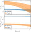 |
Fig. 17. Upper panel: dependence of |


In Table 2, we summarize the best-fit parameters describing the evolution of the quantities investigated in this paper, assuming the power-law behavior X = n ⋅ (1 + z)−γ, which are also shown in Fig. 17. Our results confirm the early-enrichment scenario suggested by recent works, with the majority of iron mass in the ICM of massive galaxy clusters produced at epochs earlier than z ∼ 1. Significant evolution is limited to the central peak component which, despite its contributing a minor fraction of the total iron mass, shows a ∼2σ significant decrease with redshift and a large intrinsic scatter. The overall picture of the iron distribution and its evolution, as we obtained in this work, will be important in extending our analysis to the total Chandra archive to include lower S/N data, therefore reaching a larger mass and redshift range. Another important extension of this work would be provided by the XMM-Newton data, which is already available for a fraction of our sample. This addition will be important to have a better handle on the iron plateau at large radii. Next future facilities, like XRISM, may provide further relevant information on the outer regions, despite the limited effective area and the small field of view (3 × 3 arcmin2) but only with a significant investment of observing time on a few, selected nearby targets. Only future (∼2030) X-ray facilities with an X-ray bolometer on board, such as Athena with X-IFU or Lynx, with its far better angular resolution, will provide high-quality observations for a large number of high redshift clusters and promise to provide a coherent picture of the chemical evolution of the ICM.
Best-fit parameters describing the evolution of the quantities investigated in this paper, assuming the power-law behavior X = n ⋅ (1 + z)−γ.
All the clusters observed with ACIS-S only have z > 0.08.
The X-ray Imaging and Spectroscopy Mission (XRISM), formerly named the “X-ray Astronomy Recovery Mission” (XARM), is a JAXA/NASA collaborative mission, with ESA participation (see Guainazzi & Tashiro 2018, and references therein), expected to be launched in 2022.
A global value can be obtained for a number of net counts in the 0.5–7 keV band as low as 1000.
We do not discuss two potential sources of systematics such as the calibration of the X-ray instruments and the plasma code used to fit the data, both of which are expected to affect the iron abundance at the level of few percent (see Molendi et al. 2016, and references therein).
The sample of Maughan et al. (2008) consists of 115 clusters, in which 111 clusters have measurements of metallicity within the extraction radius [0.15–1]r500.
Acknowledgments
We thank the anonymous referee for a constructive report that helped in improving the paper. A.L., P.T., and S.E. acknowledge financial contribution from the agreement ASI-INAF n.2017-14-H.0. PT acknowledges financial contribution from the Istituto Nazionale di Astrofisica (INAF) PRIN-SKA 2017 program 1.05.01.88.04 (ESKAPE). S.E. acknowledges financial contribution from the contracts ASI 2015-046-R.0, and from INAF “Call per interventi aggiuntivi a sostegno della ricerca di main stream di INAF”.
References
- Allen, S. W., Evrard, A. E., & Mantz, A. B. 2011, ARA&A, 49, 409 [NASA ADS] [CrossRef] [Google Scholar]
- Anders, E., & Grevesse, N. 1989, Geochim. Cosmochim. Acta, 53, 197 [Google Scholar]
- Anderson, M. E., Bregman, J. N., Butler, S. C., & Mullis, C. R. 2009, ApJ, 698, 317 [NASA ADS] [CrossRef] [Google Scholar]
- Andrade-Santos, F., Jones, C., Forman, W. R., et al. 2017, ApJ, 843, 76 [NASA ADS] [CrossRef] [Google Scholar]
- Arnaud, K. A. 1996, in Astronomical Data Analysis Software and Systems V, eds. G. H. Jacoby, & J. Barnes, ASP Conf. Ser., 101, 17 [NASA ADS] [Google Scholar]
- Asplund, M., Grevesse, N., Sauval, A. J., & Scott, P. 2009, ARA&A, 47, 481 [NASA ADS] [CrossRef] [Google Scholar]
- Baldi, A., Ettori, S., Mazzotta, P., Tozzi, P., & Borgani, S. 2007, ApJ, 666, 835 [NASA ADS] [CrossRef] [Google Scholar]
- Baldi, A., Ettori, S., Molendi, S., et al. 2012, A&A, 537, A142 [NASA ADS] [CrossRef] [EDP Sciences] [Google Scholar]
- Balestra, I., Tozzi, P., Ettori, S., et al. 2007, A&A, 462, 429 [NASA ADS] [CrossRef] [EDP Sciences] [Google Scholar]
- Balucinska-Church, M., & McCammon, D. 1992, ApJ, 400, 699 [NASA ADS] [CrossRef] [Google Scholar]
- Barret, D., Decourchelle, A., Fabian, A., et al. 2020, Astron. Nachr., 341, 224 [NASA ADS] [CrossRef] [Google Scholar]
- Biffi, V., Mernier, F., & Medvedev, P. 2018a, Space Sci. Rev., 214, 123 [NASA ADS] [CrossRef] [Google Scholar]
- Biffi, V., Planelles, S., Borgani, S., et al. 2018b, MNRAS, 476, 2689 [NASA ADS] [CrossRef] [Google Scholar]
- Böhringer, H., & Werner, N. 2010, A&ARv, 18, 127 [NASA ADS] [CrossRef] [Google Scholar]
- Böhringer, H., Matsushita, K., Churazov, E., Finoguenov, A., & Ikebe, Y. 2004, A&A, 416, L21 [NASA ADS] [CrossRef] [EDP Sciences] [Google Scholar]
- Böhringer, H., Schuecker, P., Pratt, G. W., et al. 2007, A&A, 469, 363 [NASA ADS] [CrossRef] [EDP Sciences] [Google Scholar]
- Buote, D. A., & Tsai, J. C. 1995, ApJ, 452, 522 [NASA ADS] [CrossRef] [Google Scholar]
- Buote, D. A., & Tsai, J. C. 1996, ApJ, 458, 27 [NASA ADS] [CrossRef] [Google Scholar]
- Cash, W. 1979, ApJ, 228, 939 [NASA ADS] [CrossRef] [Google Scholar]
- Cassano, R., Ettori, S., Giacintucci, S., et al. 2010, ApJ, 721, L82 [NASA ADS] [CrossRef] [Google Scholar]
- De Grandi, S., & Molendi, S. 2001, ApJ, 551, 153 [NASA ADS] [CrossRef] [Google Scholar]
- De Grandi, S., & Molendi, S. 2009, A&A, 508, 565 [NASA ADS] [CrossRef] [EDP Sciences] [Google Scholar]
- De Grandi, S., Ettori, S., Longhetti, M., & Molendi, S. 2004, A&A, 419, 7 [NASA ADS] [CrossRef] [EDP Sciences] [Google Scholar]
- De Grandi, S., Santos, J. S., Nonino, M., et al. 2014, A&A, 567, A102 [NASA ADS] [CrossRef] [EDP Sciences] [Google Scholar]
- de Plaa, J. 2013, Astron. Nachr., 334, 416 [NASA ADS] [CrossRef] [Google Scholar]
- Eckert, D., Molendi, S., & Paltani, S. 2011, A&A, 526, A79 [NASA ADS] [CrossRef] [EDP Sciences] [Google Scholar]
- Eckert, D., Roncarelli, M., Ettori, S., et al. 2015, MNRAS, 447, 2198 [NASA ADS] [CrossRef] [Google Scholar]
- Ettori, S. 2000, MNRAS, 318, 1041 [NASA ADS] [CrossRef] [Google Scholar]
- Ettori, S., Donnarumma, A., Pointecouteau, E., et al. 2013, Space Sci. Rev., 177, 119 [NASA ADS] [CrossRef] [Google Scholar]
- Ettori, S., Baldi, A., Balestra, I., et al. 2015, A&A, 578, A46 [NASA ADS] [CrossRef] [EDP Sciences] [Google Scholar]
- Foreman-Mackey, D., Hogg, D. W., Lang, D., & Goodman, J. 2013, PASP, 125, 306 [CrossRef] [Google Scholar]
- Guainazzi, M., & Tashiro, M. S. 2018, ArXiv e-prints [arXiv:1807.06903] [Google Scholar]
- Hudson, D. S., Mittal, R., Reiprich, T. H., et al. 2010, A&A, 513, A37 [NASA ADS] [CrossRef] [EDP Sciences] [Google Scholar]
- Kaastra, J. S., Tamura, T., Peterson, J. R., et al. 2004, A&A, 413, 415 [NASA ADS] [CrossRef] [EDP Sciences] [Google Scholar]
- Kalberla, P. M. W., Burton, W. B., Hartmann, D., et al. 2005, A&A, 440, 775 [NASA ADS] [CrossRef] [EDP Sciences] [Google Scholar]
- Kirkpatrick, C. C., Gitti, M., Cavagnolo, K. W., et al. 2009, ApJ, 707, L69 [NASA ADS] [CrossRef] [Google Scholar]
- Kitayama, T., Bautz, M., Markevitch, M., et al. 2014, ArXiv e-prints [arXiv:1412.1176] [Google Scholar]
- Komatsu, E., Smith, K. M., Dunkley, J., et al. 2011, ApJS, 192, 18 [NASA ADS] [CrossRef] [Google Scholar]
- Lakhchaura, K., Mernier, F., & Werner, N. 2019, A&A, 623, A17 [CrossRef] [EDP Sciences] [Google Scholar]
- Leccardi, A., & Molendi, S. 2008, A&A, 487, 461 [NASA ADS] [CrossRef] [EDP Sciences] [Google Scholar]
- Lin, Y.-T., Stanford, S. A., Eisenhardt, P. R. M., et al. 2012, ApJ, 745, L3 [NASA ADS] [CrossRef] [Google Scholar]
- Liu, A., Yu, H., Tozzi, P., & Zhu, Z.-H. 2015, ApJ, 809, 27 [CrossRef] [Google Scholar]
- Liu, A., Tozzi, P., Yu, H., De Grandi, S., & Ettori, S. 2018, MNRAS, 481, 361 [NASA ADS] [CrossRef] [Google Scholar]
- Liu, A., Zhai, M., & Tozzi, P. 2019, MNRAS, 485, 1651 [CrossRef] [Google Scholar]
- Lovisari, L., & Reiprich, T. H. 2019, MNRAS, 483, 540 [NASA ADS] [CrossRef] [Google Scholar]
- Lovisari, L., Forman, W. R., Jones, C., et al. 2017, ApJ, 846, 51 [NASA ADS] [CrossRef] [Google Scholar]
- Mantz, A. B., Allen, S. W., Morris, R. G., et al. 2017, MNRAS, 472, 2877 [NASA ADS] [CrossRef] [Google Scholar]
- Mantz, A. B., Abdulla, Z., Allen, S. W., et al. 2018, A&A, 620, A2 [NASA ADS] [CrossRef] [EDP Sciences] [Google Scholar]
- Maughan, B. J., Jones, C., Forman, W., & Van Speybroeck, L. 2008, ApJS, 174, 117 [NASA ADS] [CrossRef] [Google Scholar]
- Mazzotta, P., Rasia, E., Moscardini, L., & Tormen, G. 2004, MNRAS, 354, 10 [NASA ADS] [CrossRef] [Google Scholar]
- McDonald, M., Bulbul, E., de Haan, T., et al. 2016, ApJ, 826, 124 [NASA ADS] [CrossRef] [Google Scholar]
- Merloni, A. 2012, Science from the Next Generation Imaging and Spectroscopic Surveys, 43 [Google Scholar]
- Mernier, F., de Plaa, J., Kaastra, J. S., et al. 2017, A&A, 603, A80 [NASA ADS] [CrossRef] [EDP Sciences] [Google Scholar]
- Mernier, F., Biffi, V., Yamaguchi, H., et al. 2018, Space Sci. Rev., 214, 129 [NASA ADS] [CrossRef] [Google Scholar]
- Mernier, F., Werner, N., Bagchi, J., et al. 2019, MNRAS, 486, 5430 [NASA ADS] [CrossRef] [Google Scholar]
- Molendi, S., Eckert, D., De Grandi, S., et al. 2016, A&A, 586, A32 [NASA ADS] [CrossRef] [EDP Sciences] [Google Scholar]
- Mushotzky, R. F., & Loewenstein, M. 1997, ApJ, 481, L63 [NASA ADS] [CrossRef] [Google Scholar]
- Mushotzky, R., Loewenstein, M., Arnaud, K. A., et al. 1996, ApJ, 466, 686 [NASA ADS] [CrossRef] [Google Scholar]
- Mushotzky, R., Aird, J., Barger, A. J., et al. 2019, BAAS, 51, 107 [Google Scholar]
- O’Hara, T. B., Mohr, J. J., Bialek, J. J., & Evrard, A. E. 2006, ApJ, 639, 64 [NASA ADS] [CrossRef] [Google Scholar]
- Panagoulia, E. K., Sanders, J. S., & Fabian, A. C. 2015, MNRAS, 447, 417 [NASA ADS] [CrossRef] [Google Scholar]
- Piffaretti, R., Arnaud, M., Pratt, G. W., Pointecouteau, E., & Melin, J.-B. 2011, A&A, 534, A109 [NASA ADS] [CrossRef] [EDP Sciences] [Google Scholar]
- Pratt, G. W., Croston, J. H., Arnaud, M., & Böhringer, H. 2009, A&A, 498, 361 [NASA ADS] [CrossRef] [EDP Sciences] [Google Scholar]
- Presotto, V., Girardi, M., Nonino, M., et al. 2014, A&A, 565, A126 [NASA ADS] [CrossRef] [EDP Sciences] [Google Scholar]
- Rosati, P., Tozzi, P., Gobat, R., et al. 2009, A&A, 508, 583 [NASA ADS] [CrossRef] [EDP Sciences] [Google Scholar]
- Rossetti, M., Gastaldello, F., Eckert, D., et al. 2017, MNRAS, 468, 1917 [NASA ADS] [CrossRef] [Google Scholar]
- Russell, H. R., Sanders, J. S., & Fabian, A. C. 2008, MNRAS, 390, 1207 [NASA ADS] [CrossRef] [Google Scholar]
- Sanders, J. S., & Fabian, A. C. 2007, MNRAS, 381, 1381 [NASA ADS] [CrossRef] [Google Scholar]
- Sanderson, A. J. R., O’Sullivan, E., & Ponman, T. J. 2009, MNRAS, 395, 764 [NASA ADS] [CrossRef] [Google Scholar]
- Santos, J. S., Rosati, P., Tozzi, P., et al. 2008, A&A, 483, 35 [NASA ADS] [CrossRef] [EDP Sciences] [Google Scholar]
- Santos, J. S., Tozzi, P., Rosati, P., & Böhringer, H. 2010, A&A, 521, A64 [NASA ADS] [CrossRef] [EDP Sciences] [Google Scholar]
- Santos, J. S., Tozzi, P., Rosati, P., Nonino, M., & Giovannini, G. 2012, A&A, 539, A105 [NASA ADS] [CrossRef] [EDP Sciences] [Google Scholar]
- Schellenberger, G., Reiprich, T. H., Lovisari, L., Nevalainen, J., & David, L. 2015, A&A, 575, A30 [NASA ADS] [CrossRef] [EDP Sciences] [Google Scholar]
- Serlemitsos, P. J., Smith, B. W., Boldt, E. A., Holt, S. S., & Swank, J. H. 1977, ApJ, 211, L63 [NASA ADS] [CrossRef] [Google Scholar]
- Simionescu, A., Werner, N., Böhringer, H., et al. 2009, A&A, 493, 409 [NASA ADS] [CrossRef] [EDP Sciences] [Google Scholar]
- Simionescu, A., Werner, N., Urban, O., et al. 2013, ApJ, 775, 4 [NASA ADS] [CrossRef] [Google Scholar]
- Simionescu, A., Werner, N., Mantz, A., Allen, S. W., & Urban, O. 2017, MNRAS, 469, 1476 [NASA ADS] [CrossRef] [Google Scholar]
- Smith, R. K., Brickhouse, N. S., Liedahl, D. A., & Raymond, J. C. 2001, ApJ, 556, L91 [NASA ADS] [CrossRef] [Google Scholar]
- Sun, M., Voit, G. M., Donahue, M., et al. 2009, ApJ, 693, 1142 [NASA ADS] [CrossRef] [Google Scholar]
- Tamura, T., Maeda, Y., Mitsuda, K., et al. 2009, ApJ, 705, L62 [NASA ADS] [CrossRef] [Google Scholar]
- Thölken, S., Lovisari, L., Reiprich, T. H., & Hasenbusch, J. 2016, A&A, 592, A37 [NASA ADS] [CrossRef] [EDP Sciences] [Google Scholar]
- Tozzi, P., Rosati, P., Ettori, S., et al. 2003, ApJ, 593, 705 [NASA ADS] [CrossRef] [Google Scholar]
- Tozzi, P., Santos, J. S., Nonino, M., et al. 2013, A&A, 551, A45 [NASA ADS] [CrossRef] [EDP Sciences] [Google Scholar]
- Tozzi, P., Santos, J. S., Jee, M. J., et al. 2015, ApJ, 799, 93 [NASA ADS] [CrossRef] [Google Scholar]
- Urban, O., Werner, N., Allen, S. W., Simionescu, A., & Mantz, A. 2017, MNRAS, 470, 4583 [NASA ADS] [CrossRef] [Google Scholar]
- Urdampilleta, I., Mernier, F., Kaastra, J. S., et al. 2019, A&A, 629, A31 [CrossRef] [EDP Sciences] [Google Scholar]
- Vikhlinin, A. 2019, BAAS, 51, 30 [Google Scholar]
- Vikhlinin, A., Markevitch, M., Forman, W., & Jones, C. 2001, ApJ, 555, L87 [NASA ADS] [CrossRef] [Google Scholar]
- Vikhlinin, A., Kravtsov, A., Forman, W., et al. 2006, ApJ, 640, 691 [NASA ADS] [CrossRef] [Google Scholar]
- Vikhlinin, A., Burenin, R. A., Ebeling, H., et al. 2009, ApJ, 692, 1033 [NASA ADS] [CrossRef] [Google Scholar]
- Werner, N., Urban, O., Simionescu, A., & Allen, S. W. 2013, Nature, 502, 656 [NASA ADS] [CrossRef] [Google Scholar]
- Willingale, R., Starling, R. L. C., Beardmore, A. P., Tanvir, N. R., & O’Brien, P. T. 2013, MNRAS, 431, 394 [NASA ADS] [CrossRef] [Google Scholar]
- Willis, J. P., Canning, R. E. A., Noordeh, E. S., et al. 2020, Nature, 577, 39 [CrossRef] [Google Scholar]
Appendix A: Properties of the sample
In Table A.1, we list the results of our spectral analysis for the global quantities of the entire cluster sample. The 186 clusters (including the 16 clusters discarded from the final analysis because of the irregular abundance profile) are listed in alphabetical order according to the target name. The positions correspond to the X-ray centroid identified as described in Sect. 2.2. We report the X-ray redshift, which is the value used in our analysis, and the core-excised temperature, which is the emission-weighted value obtained fitting the projected emission in the range (0.1–0.4)r500 with a single apec model. M500 is the total halo mass obtained from Eqs. (2) and (3), while the ICM mass within r500 is measured directly from the deprojected ICM density profile integrated over the spherical volume within r500. Finally, we list the three abundance measurements used in this work: the emission-weighted iron abundance within 0.4r500, and the gas mass-weighted iron abundance within 0.4r500 and r500.
Global properties we measured for the 186 clusters.
All Tables
Slope of the relation between average abundance and redshift from the literature compared to the values found in this work.
Best-fit parameters describing the evolution of the quantities investigated in this paper, assuming the power-law behavior X = n ⋅ (1 + z)−γ.
All Figures
|
Fig. 1. General properties of the cluster sample used in this work (186 clusters). Upper left: X-ray redshift measured in this work compared to the optical redshift from the literature. Lower left: distribution of the redshift of the clusters in our sample. Upper right: distribution of the emission-weighted (spectroscopic-like) temperature in the radial range [0.1, 0.4]r500 across the sample. Lower right: distribution of M500, estimated according to Eq. (3), plotted versus redshift. |
| In the text | |
|
Fig. 2. Distribution of the surface brightness concentration cSB of the clusters in the full sample and in 4 independent redshift bins with roughly the same number of clusters (N). The vertical dashed lines indicate the threshold for non-cool-core and weak cool-core clusters: cSB = 0.075 and cSB = 0.155. |
| In the text | |
|
Fig. 3. Projected iron abundance profiles for all the clusters in our sample. Each point, color-coded by redshift, is the best-fit value in the corresponding radial bin. For clarity error bars are shown in light grey. The yellow points show the sample-average abundance and rms within seven radial bins. |
| In the text | |
|
Fig. 4. Left panel: best-fit double-β model of the deprojected density profiles, color-coded by redshift, for all the clusters in our sample. Right panel: total iron mass profiles obtained by convolving the gas density profile with the best fit abundance profile for each cluster in our sample. At r > 0.4r500 the iron mass is computed extrapolating the constant plateau up to r500. |
| In the text | |
|
Fig. 5. Probability of rejection of the abundance profiles with and without the iron plateau. The dashed lines mark (1 − P) = 0.90, hence the yellow points shows clusters for which both the single- and double-component models are rejected at >90% c.l. Clusters colored in red favor the double-component model, while both models provide similar quality fits to the clusters colored in blue. In these cases, the double-component model returns a slightly lower goodness because of the inclusion of an additional parameter in the fit. |
| In the text | |
|
Fig. 6. Examples of abundance profiles with the corresponding double-component (red) and single-component (blue) best-fit models. From left to right: Abell 2050, CLJ1415+3612, and PSZ2 G241.77−24.00. The three examples are extracted from the yellow, red, and blue dots in Fig. 5, which are clusters that: cannot be fitted with either model (yellow); favor the double-component model (red); and can be fitted with both models in the observed radial range (blue). The best-fit values and uncertainties (of all the curve fittings in this paper, unless noted otherwise) are obtained using the MCMC tool of Foreman-Mackey et al. (2013). |
| In the text | |
|
Fig. 7. Iron abundance profile of MACSJ0242.5−2132 with the best-fit showing a pronounced central iron drop. The red, cyan, and blue curves are the iron peak, iron drop, and iron plateau, respectively, as described by Eq. (8). |
| In the text | |
|
Fig. 8. Left panel: correlation between the average, gas mass-weighted iron abundance (within r500) and the redshift of all the clusters. The black curve and shaded area show the best-fit function Zmw = Zmw, 0 ⋅ (1 + z)−γmw with Zmw, 0 = (0.38 ± 0.03) Z⊙ and γmw = 0.28 ± 0.31. Right panel: gas mass-weighted abundance within 0.4r500 plotted against the emission-weighted value in the same radial range. The solid line corresponds to Zmw = Zew. Dashed lines show the average relation for cool-core and non-cool-core clusters, |
| In the text | |
|
Fig. 9. Left panel: cumulative iron mass profiles corresponding to the peak component, color-coded by redshift for all the 170 clusters with regular abundance profiles considered in this work. Right panel: as in the left panel, but for the plateau component. |
| In the text | |
|
Fig. 10. Distribution of the ratio of iron peak mass to iron plateau mass within r500, and the correlation with redshift. The green dashed line indicates the weighted average at ∼0.008. The black dashed lines mark the [5 × 10⁻⁵, 0.5] range roughly corresponding to >90% of the clusters symmetrically distributed around the central value (as shown in the left-side panel). |
| In the text | |
|
Fig. 11. Upper left: distribution of the abundance of the iron plateau component Zplateau. The dashed line indicates the weighted average value ⟨Zplateau⟩ = 0.38 Z⊙. The dashed curve shows a normalized Gaussian with σ = 0.11 Z⊙, corresponding to the average statistical error, and μ = 0.38 Z⊙, corresponding to the weighted average value. Upper right: abundance of the iron plateau plotted against cluster redshift. The black curve and shaded area show the best-fit function Zplateau = Zplateau, 0 ⋅ (1 + z)−γplateau with Zplateau, 0 = (0.41 ± 0.02) Z⊙ and γplateau = 0.21 ± 0.18, which are obtained by fitting the weighted average values and uncertainties of the four bins shown as blue solid lines and shaded areas. Lower left: distribution of the normalization of the iron peak component Zpeak. The dashed line indicates the weighted average value ⟨Zpeak⟩ = 0.52 Z⊙. The dashed curve shows a normalized Gaussian with σ = 0.42 Z⊙, corresponding to the average statistical error, and μ = 0.52 Z⊙, corresponding to the weighted average value. Lower right: normalization of the iron peak component Zpeak plotted against cluster redshift. The black curve and shaded area show the best-fit function Zpeak = Zpeak, 0 ⋅ (1 + z)−γpeak with Zpeak, 0 = (0.68 ± 0.07) Z⊙ and γpeak = 0.79 ± 0.53. |
| In the text | |
|
Fig. 12. Upper panels: ratio of iron mass of the plateau (left) and the peak (right) to the gas mass within r500 versus cluster redshift. The black curves show the best-fit functions |
| In the text | |
|
Fig. 13. Left: correlation between gas mass-weighted abundance within r500 and the total mass M500 for all the clusters in the sample. The black curve and shaded area denote the best fit function and the 1σ confidence interval: Zmw = (0.52 ± 0.08)⋅(M500/1014 M⊙)−0.14 ± 0.09. Right: correlation between the gas mass and M500. The black curve and shaded area denote the best fit function and the 1σ confidence interval: Mgas/1014 M⊙ = (0.131 ± 0.012)⋅(M500/1014 M⊙)1.05 ± 0.06. |
| In the text | |
|
Fig. 14. Comparison between the gas mass-weighted abundance measured in this work and the emission-weighted abundance provided by Maughan et al. (2008), for the overlapping 48 clusters. The reference solar abundance for the data points of Maughan et al. (2008) has been adjusted from Anders & Grevesse (1989) to Asplund et al. (2009), for a direct comparison with our results. |
| In the text | |
|
Fig. 15. Projected and deprojected iron abundance profiles of Abell 383: an example to show the impact of projection effect. The iron peak and iron plateau components in the best-fit model are plotted with dash-dotted lines and dashed lines, respectively. |
| In the text | |
|
Fig. 16. Upper panel: comparison of the measured nH, free and nH, tot. The nH values are in units of 1022 cm−2. The vertical dashed line denotes 0.05 × 1022 cm−2. The solid line corresponds to nH, free = nH, tot. Lower panel: ratio of all the best-fit abundance values obtained by adopting our strategy in nH (free to vary in a limited interval around nH, free) and by fixing nH to nH, tot, as a function of nH, tot. |
| In the text | |
|
Fig. 17. Upper panel: dependence of |
| In the text | |
Current usage metrics show cumulative count of Article Views (full-text article views including HTML views, PDF and ePub downloads, according to the available data) and Abstracts Views on Vision4Press platform.
Data correspond to usage on the plateform after 2015. The current usage metrics is available 48-96 hours after online publication and is updated daily on week days.
Initial download of the metrics may take a while.