| Issue |
A&A
Volume 694, February 2025
|
|
|---|---|---|
| Article Number | A149 | |
| Number of page(s) | 18 | |
| Section | Numerical methods and codes | |
| DOI | https://doi.org/10.1051/0004-6361/202451431 | |
| Published online | 07 February 2025 | |
The clus model in SPEX: Projection and resonant scattering effects on the iron abundance and temperature profiles of galaxy clusters
1
Leiden Observatory, Leiden University,
PO Box 9513,
2300RA
Leiden,
The Netherlands
2
SRON Netherlands Institute for Space Research,
Niels Bohrweg 4,
2333
CA
Leiden,
The Netherlands
3
Department of Theoretical Physics and Astrophysics, Faculty of Science, Masaryk University,
Kotlářská 2,
Brno
611 37,
Czech Republic
4
Kavli Institute for the Physics and Mathematics of the Universe, The University of Tokyo, Kashiwa,
Chiba
277-8583,
Japan
★ Corresponding author; This email address is being protected from spambots. You need JavaScript enabled to view it.
Received:
9
July
2024
Accepted:
11
December
2024
Abstract
In this paper we introduce the clus model, which has been newly implemented in the X-ray spectral fitting software package SPEX. Based on 3D radial profiles of the gas density, temperature, and metal abundance as well as the turbulent, inflow, and outflow velocities, the clus model creates spectra for a chosen projected region on the sky. Additionally, it can also take into account the resonant scattering. We show a few applications of the clus model on simulated spectra of the massive elliptical galaxy NGC 4636; galaxy clusters A383, A2029, A1795, and A262; and the Perseus cluster. We quantify the effect of projection as well as the resonant scattering on inferred profiles of the iron abundance and temperature, assuming a resolution similar to Chandra ACIS-S and XRISM Resolve. Our results show that depending on the mass of the object as well as the projected distance from its core, neither a single-temperature or double-temperature model nor the Gaussian-shaped differential emission measure model can accurately describe the input emission measure distribution of these massive objects. The largest effect of projection as well as resonant scattering was observed for projected profiles of iron abundance of NGC 4636, which is where we could reproduce the observed iron abundance drop in its innermost few kiloparsecs. Furthermore, we find that projection effects also influence the best-fit temperature, and the magnitude of this effect varies depending on the underlying hydrodynamical profiles of individual objects. In the core, the projection effects are the largest for A1795 and NGC 4636, while in the outskirts, the largest difference between 2D and 3D temperature profiles is for Perseus and A1795, regardless of the instrumental resolution. These findings might potentially have an impact on cross-calibration studies between different instruments as well as on the precision cosmology.
Key words: scattering / techniques: spectroscopic / galaxies: clusters: general / galaxies: clusters: intracluster medium / X-rays: galaxies: clusters
© The Authors 2025
 Open Access article, published by EDP Sciences, under the terms of the Creative Commons Attribution License (https://creativecommons.org/licenses/by/4.0), which permits unrestricted use, distribution, and reproduction in any medium, provided the original work is properly cited.
This article is published in open access under the Subscribe to Open model. This email address is being protected from spambots. You need JavaScript enabled to view it. to support open access publication.
1 Introduction
Galaxy clusters, galaxy groups, and massive elliptical galaxies appear as diffused sources of light at X-ray wavelengths (Forman et al. 1972; Kellogg et al. 1972). Plasma revealed in this way by X-ray emission is referred to as the intracluster medium (ICM), the intragroup medium (IGrM), or the circumgalactic medium (CGM) and forms a major fraction of the baryonic matter in all these mentioned objects. This X-ray plasma emits mostly through the free-free continuum (thermal bremsstrahlung) and through line emission. The X-ray spectroscopy of these sources can be used to derive many of their properties, for example, their electron temperature, electron density, turbulent velocities, and metal abundances (Böhringer & Werner 2010).
In the past few decades, the capabilities of X-ray spectroscopy have mainly been showcased through charged coupled device (CCD) and grating spectrometers. The Chandra X-ray Observatory, XMM-Newton, and Suzaku have allowed great progress thanks to their improved spectral and spatial resolution as well as larger effective area and low background. X-ray spectroscopy also reached a notable milestone in 2016 when a micro-calorimeter on board the Hitomi satellite was launched, which offered an unprecedented spectral resolution of 5 eV at the energy of 6 keV. More recently, XRISM was launched into its orbit in September 2023. It carries on the legacy of Hitomi and will continue observing the Universe through high-resolution spectroscopy.
Among the many discoveries enabled with Chandra, XMM-Newton, and Suzaku, these observatories have provided detailed measurements of the metal distribution in galaxy clusters, galaxy groups, and giant elliptical galaxies. Many of these objects show flattened or peaky metal (mostly iron) abundance profiles towards their cores; however, X-ray observations of some of them revealed a steep decrease (sometimes by as much as 50% of their global maximum) of metal abundances in the few innermost kiloparsecs (Churazov et al. 2003; Johnstone et al. 2002; Sanders & Fabian 2002, 2007; Million et al. 2010; Rafferty et al. 2013; Mernier et al. 2017).
A few possible scenarios have arisen to explain these central abundance drops but their origin has not yet been established. For example, metals can be transported to larger distances by the mechanical energy powered by the active galactic nucleus (AGN) feedback (Simionescu et al. 2008, 2009) or by galactic winds (Schindler et al. 2005). Studies by Panagoulia et al. (2013, 2015) have suggested instead that iron might get depleted into dust grains in the cores of these massive objects, and therefore it becomes ‘invisible’ in X-rays. If this scenario is true and if elements such as iron, silicon, sulphur, magnesium, or calcium show the central abundance drop, the noble gases such as neon or argon should be indifferent to this process. Such behaviour has been confirmed with Chandra in Lakhchaura et al. (2019), who report that in the central 10 kpc of the Centaurus galaxy cluster, elements such as Fe, Si, S, Mg, and Ca show an abundance drop. However, no abundance drop was found in Ar. Liu et al. (2019) found similar results for ten cool-core clusters. Contrary to these conclusions, measurements with XMM-Newton have suggested that the observed abundance drop in the Centaurus cluster could be partly caused by systematic uncertainties in the atomic data and response matrices, rather than the depletion of iron into dust (Fukushima et al. 2022). Future XRISM observations of metals in the Centaurus galaxy cluster promise to resolve this mystery. Other scenarios originate from the incompleteness of the spectral fitting models, for example projection effects (Sanders & Fabian 2007), modelling of the central brightest cluster galaxy (BCG), or a simplification of the multi-temperature plasma with a single-temperature fitting model, which is also known as the ‘iron bias’ (Buote 2000). Another scenario suggests sedimentation of helium nuclei in the cluster cores, which could potentially raise the helium abundance values above the solar one and therefore overestimate the continuum and underestimate all other abundances (Ettori & Fabian 2006). This scenario is, however, impossible to test directly in X-rays since He does not have transitions in X-ray wavelengths.
An alternative explanation arose from an idea proposed in Gilfanov et al. (1987), which shows that the radial X-ray surface brightness profile of galaxy clusters can be distorted by the scattering of X-ray photons in the resonant lines of highly charged and heavy-metal ions. Some lines in the ICM have optical depths larger than unity and undergo the resonant scattering (RS) process. If a photon is resonantly scattered, it gets absorbed and almost immediately re-emitted in a different direction. This causes the flux in the resonant line to drop in the cluster cores; however, in the outskirts, the flux of the same resonant line is enhanced. Since the optical depth of each spectral line also depends, among other things, on the turbulent velocity, RS has been used as an independent proxy to measure gas motions and turbulent velocities in the ICM and IGrM, in addition to the gas velocities obtained from the line broadening (see e.g. Churazov et al. 2004; Werner et al. 2009; de Plaa et al. 2012; Zhuravleva et al. 2013; Ogorzalek et al. 2017; Gu et al. 2018). A recent study of Nelson et al. (2023) has shown that RS could be used to observe the CGM around galaxies with future X-ray observatories. Additionally, RS has been studied in relation to the abundance drop in the Centaurus galaxy cluster. However, Sanders & Fabian (2006) showed that accounting for RS does not remove the central dip in its abundance profile. In the case of the massive elliptical galaxy NGC 4636, Werner et al. (2009) concluded that neglecting the effect of RS underestimates the chemical abundances of iron and oxygen by around 10–20%.
In this paper, we present the clus model, which has been newly implemented in the SPEctral X-ray and EUV (SPEX) software package and which calculates the spectrum and radial profiles for a spherically symmetric approximation of a cluster or a group of galaxies, or even massive elliptical galaxies. In Sect. 2, we describe details of this model, our sample selection, and the fitting procedure. In Sect. 3, we provide an application of the clus model to the Chandra ACIS-S and XRISM Resolve simulated data, and we address whether the clus model can help with understanding the origin of the iron abundance drops in the cores of some galaxy clusters, groups, or giant elliptical galaxies. We also discuss the effects on the projected temperature profiles. In Sect. 4, we discuss our results and compare our findings to existing literature studies. Lastly, Sect. 5 summarises our main conclusions.
2 Methods
2.1 SPEX
We used the SPEX software package (Kaastra et al. 1996; Kaastra et al. 2018, 2020) version 3.081 for modelling and analysis of high-resolution X-ray spectra. With its own atomic database, the SPEX Atomic Code & Tables (SPEXACT), it includes around 4.2 × 10⁶ lines from 30 different chemical elements (H to Zn). Since the first version of SPEX, many updates have been made, including the implementation of the clus model, which is described in more detail in this paper. Unless stated otherwise, we use the proto-solar abundances by Lodders et al. (2009).
2.2 The clus model
The clus model takes as input parametrised 3D radial profiles of the gas density, temperature, and metal abundance as well as the turbulent, inflow, and outflow velocities. Given these parametrised profiles, the emission in multiple 3D shells – each approximated as a single temperature model in collisional ionisation equilibrium (CIE) – is computed and projected onto the sky. The number of shells can be adjusted and is set by a user through the parameters nr (number of 3D shells for which the model is evaluated) and npro (number of projected annuli). The 3D model is evaluated on a logarithmically spaced grid, which is defined by the inner radius rin and outer radius rout, where at radius rout the density is set to zero. Radius rin is taken as 1% of r500, or if it is smaller, 10% of the smallest of the core radii in the density profile (see Sect. 2.2.1). For the innermost shell, the inner boundary rin is replaced by zero. The clus model can then be run in different modes, where the output is either the spectral energy distribution within a user-defined projected spatial region or a radial surface brightness profile in a user-requested energy band. More specifically, the assumed shapes of the underlying 3D profiles used as input in the clus model follow a two β model for the density distribution (with the additional possibility to introduce a jump or a break in the slope at a given radius; see Sect. 2.2.1); the same functional form for the temperature profile as that proposed in Vikhlinin et al. (2006), again with a possible additional jump (see Sect. 2.2.2), and the universal abundance profile as defined in Mernier et al. (2017) (see Sect. 2.2.3).
The hydrodynamical profiles such as density or temperature are evaluated for the middle radius of each shell using analytical parametrisation of the 3D profiles, and it is assumed that these quantities are constant within the shell. Therefore, the emission measure of each shell is simply evaluated as the product of electron and hydrogen density at the central radius of the shell multiplied by the volume of the shell. In case the user introduces a density discontinuity in the model, the radius of the density discontinuity is also chosen as an additional grid point; if it is close to an existing grid point, that existing grid point is moved to the discontinuity.
The clus model takes a linear grid for the projected 2D profiles, which emulates real detectors that are designed with a linear scale. For the 3D profiles, the quantities are evaluated at the shell central radii, while for the 2 D projected profiles the quantities are evaluated at sub-shell resolution (typically using 20 points for each shell). Within the shell, it is assumed that the emission measure as a function of radius follows a power law. The power-law slope is determined by comparing the emission measures of the neighbouring shells.
The clus model also has two ascii-output options: (a) the output clus gives the radius, hydrogen density, temperature, gas pressure, emission measure, turbulent velocity, outflow velocity, and relative abundances, and (b) the output clup provides the projected radial profile of the number of photons and energy flux in an energy band that is specified with parameters Emin and Emax (given in units of keV). The clus model has in total 80 different parameters, which are summarised in Table A.1.
2.2.1 Radial density profile
The hydrogen density distribution nH(r) is parametrised as the sum of two beta models (Cavaliere & Fusco-Femiano 1976; Mohr et al. 1999), modified by a possible density jump:
![Mathematical equation: $\[n_{\mathrm{H}}(r)=\left[n_{1}(r)+n_{2}(r)\right] \times f(r).\]$](/articles/aa/full_html/2025/02/aa51431-24/aa51431-24-eq1.png) (1)
(1)
Densities ni(r), where i = 1, 2, are defined as
![Mathematical equation: $\[n_{i}(r)=\frac{n_{0, i}}{\left[1+\left(r / r_{c, i}\right)^{2}\right]^{1.5 \beta_{i}}},\]$](/articles/aa/full_html/2025/02/aa51431-24/aa51431-24-eq2.png) (2)
(2)
where n0,1 and n0,2 are the central densities, rc,1 and rc,2 are the core radii, and β1 and β2 are the slopes of the beta profiles. The optional density jump f(r) is defined as
![Mathematical equation: $\[\begin{aligned}& r<r_s: f(r)=1 \\& r>r_s: f(r)=\Delta_d\left(r / r_s\right)^{\gamma_d},\end{aligned}\]$](/articles/aa/full_html/2025/02/aa51431-24/aa51431-24-eq3.png) (3)
(3)
where rs is the discontinuity radius and Δd is the density jump at rs. For Δd > 1, the density increases outside rs relative to the undisturbed profile, while for Δd < 1 it decreases. Further fine-tuning of this thermodynamic discontinuity (which can represent, e.g. a shock or a cold front) can be achieved by changing the power-law parameter γd. If γd > 0 (γd < 0), the values are increasing (decreasing) at large radii, while γd = 0 means a constant jump.
2.2.2 Radial temperature profile
The temperature profile T(r) can be written as
![Mathematical equation: $\[T(r)=T_{1}(r) \times f_{1}(r) \times f_{2}(r),\]$](/articles/aa/full_html/2025/02/aa51431-24/aa51431-24-eq4.png) (4)
(4)
where T1(r) is based on Vikhlinin et al. (2006) (Eq. (6)) and is re-written to a different but equivalent form following Eq. (10) in Kaastra et al. (2004)
![Mathematical equation: $\[\begin{aligned}T_1(r) & =T_c+\left(T_h-T_c\right) \frac{\left(r / r_{t c}\right)^\mu}{1+\left(r / r_{t c}\right)^\mu} \\f_1(r) & =\frac{\left(r / r_{t o}\right)^{-a}}{\left[1+\left(r / r_{t o}\right)^b\right]^{c / b}}.\end{aligned}\]$](/articles/aa/full_html/2025/02/aa51431-24/aa51431-24-eq5.png) (5)
(5)
The central and outer temperatures Tc and Th, respectively, are not the actual temperatures but the temperatures that would exist without the f1(r) and f2(r) terms. The temperature jump f2(r) is defined as
![Mathematical equation: $\[\begin{aligned}& r<r_s: f_2(r)=1, \\& r>r_s: f_2(r)=\Delta_t\left(r / r_s\right)^{\gamma_t},\end{aligned}\]$](/articles/aa/full_html/2025/02/aa51431-24/aa51431-24-eq6.png) (6)
(6)
where Δt and γt are the temperature jump and the power-law parameter, which are defined similarly to the density jump, and the discontinuity radius rs is the same as for the jump in the density profile. We assume that the ion temperature is equal to the electron temperature for each shell. If one aims to relate the clus model temperature parameters to those of Vikhlinin et al. (2006), then
![Mathematical equation: $\[T_{c}=T_{\min }, T_{h}=T_{0}, \mu=a_{\mathrm{cool}}, r_{t c}=r_{\mathrm{cool}}, r_{t o}=r_{t},\]$](/articles/aa/full_html/2025/02/aa51431-24/aa51431-24-eq7.png) (7)
(7)
where Tmin, T0, acool, rcool, and rt are parameters from Eqs. (4) and (5) in Vikhlinin et al. (2006).
2.2.3 Radial abundance profile
The relative metal abundances from hydrogen to zinc (parameters 01 to 30 in the clus model) are given in proto-solar units, where the user can specify which set of abundance tables is used (see the SPEX command ‘abundance’). By default, the reference element that serves as a scaling atom is hydrogen, but it can also be specified by the user. These abundances can be modified by a multiplicative radial scaling law fabu(r) whose form is a modified version of Eq. (6) from Mernier et al. (2017)
![Mathematical equation: $\[f_{\mathrm{abu}}(r)=\frac{A}{(1+r / B)^{C}}\left[1-D \exp ^{-(r / F) \times(1+r / E)}\right]+G,\]$](/articles/aa/full_html/2025/02/aa51431-24/aa51431-24-eq8.png) (8)
(8)
where the default values for parameters (A = 1.34, B = 0.021, C = 0.48, D = 0.414, E = 0.163, and F = 0.0165) are set to the universal abundance profile values from Mernier et al. (2017). If the abundances are meant to be constant as a function of radius, the user should take care that f(r) ≡ 1 for all radii. This can be achieved for instance by setting A = 0 and G = 1. The constant term G was not included in Mernier et al. (2017) but may be useful for some applications. The radial scaling works the same way for all chemical elements (i.e. all elements are assumed to have the same radial profile shape); the abundances themselves can be different. The radial scaling is only done for elements with a nuclear charge of three or more (i.e. lithium and higher). Hydrogen and helium are excluded from the scaling. It is therefore highly recommended to keep the reference atom at its default (hydrogen) for this model.
2.2.4 Turbulent velocity and radial motions of plasma
The turbulent velocity vturb is defined as
![Mathematical equation: $\[v_{\text {turb}}^{2}(r)=v_{a}^{2}+\frac{v_{b}\left|v_{b}\right| \times\left(r / r_{v}\right)^{2}}{1+\left(r / r_{v}\right)^{2}},\]$](/articles/aa/full_html/2025/02/aa51431-24/aa51431-24-eq9.png) (9)
(9)
and it is equivalent to the root-mean-square velocity vrms, which is related to the micro-turbulent velocity vmic following a relation
![Mathematical equation: $\[v_{\text {mic }}=\sqrt{2} v_{\text {rms }}=\sqrt{2} v_{\text {turb}}.\]$](/articles/aa/full_html/2025/02/aa51431-24/aa51431-24-eq10.png) (10)
(10)
The Doppler broadening ΔED of a line with a rest frame energy E0 is then expressed as
![Mathematical equation: $\[\Delta E_{D}=\frac{E_{0}}{c} \sqrt{\left(\frac{2 k_{B} T_{\text {ion}}}{A m_{p}}+v_{\text {mic}}^{2}\right)},\]$](/articles/aa/full_html/2025/02/aa51431-24/aa51431-24-eq11.png) (11)
(11)
where c is the speed of light, kB is the Boltzmann constant, A is the atomic weight, mp is the mass of a proton, and Tion is the ion temperature. The term ![Mathematical equation: $\[\sqrt{\frac{2 k_{B} T_{\text {ion }}}{A m_{p}}}\]$](/articles/aa/full_html/2025/02/aa51431-24/aa51431-24-eq12.png) represents the thermal broadening.
represents the thermal broadening.
At the centre, vturb is given by vturb = va; at large distances, it is given by ![Mathematical equation: $\[v_{\text {turb }}^{2}=v_{a}^{2}+v_{b}\left|v_{b}\right|\]$](/articles/aa/full_html/2025/02/aa51431-24/aa51431-24-eq13.png) . Positive values of vb mean increasing turbulence for larger radii, while negative values of vb mean decreasing turbulence for larger radii. To be more precise, we emphasise that the turbulent velocity as defined in Eq. (9) refers to the standard deviation of the velocities within each radial bin, including both microscopic and macroscopic gas motions. In addition, the thermal motions of the ion are added in quadrature using the relevant (ion) temperature. We note that for negative values of vb with vb < −va, the turbulent velocity would become imaginary (v2 < 0). To avoid a crash, SPEX cuts these values off to zero and continues its calculations.
. Positive values of vb mean increasing turbulence for larger radii, while negative values of vb mean decreasing turbulence for larger radii. To be more precise, we emphasise that the turbulent velocity as defined in Eq. (9) refers to the standard deviation of the velocities within each radial bin, including both microscopic and macroscopic gas motions. In addition, the thermal motions of the ion are added in quadrature using the relevant (ion) temperature. We note that for negative values of vb with vb < −va, the turbulent velocity would become imaginary (v2 < 0). To avoid a crash, SPEX cuts these values off to zero and continues its calculations.
In addition to turbulence, the model allows for systematic radial motion (inflow or outflow), which is defined as
![Mathematical equation: $\[v_{\mathrm{rad}}(r)=v_{c}+\frac{\left(v_{h}-v_{c}\right) \times\left(r / r_{z}\right)^{2}}{1+\left(r / r_{z}\right)^{2}},\]$](/articles/aa/full_html/2025/02/aa51431-24/aa51431-24-eq14.png) (12)
(12)
where parameter vc corresponds to the flow velocity at the core and vh is the flow velocity at large distances. Positive values of vrad correspond to the inflow, and negative values correspond to the outflow. Radii rv and rz are typical radii where the velocity fields (vturb, vrad) change.
2.2.5 Projection of the radial profiles
The clus model projects the spectra of all shells onto the sky. Instead of the spectrum for the full cluster, users can also specify calculation of the spectrum within a projected annulus, which is given by the inner (rmin) and outer (rmax) radii in units of rout. As previously mentioned, at radius rout, the density is set to zero. Thus, for rmin = 0 and rmax = 1, the full cluster spectrum is obtained.
If the user wants to calculate the spectrum or profile in a more complex region and not a simple annulus, for instance, the projection of a square detector (pixel), the clus model provides this option by using the parameter azim. For azim=0, the full annulus is used, while for azim=1, a more complex region can be used. In this latter case, the user must specify the name of an ascii-file through the parameter called fazi, which describes the covered azimuthal fraction of the desired region as a function of radius. For a more detailed description of the specific format of this ascii-file, we refer the reader to Sect. 4.1.6.10 of the SPEX manual2.
2.2.6 Resonance scattering
The resonance scattering (RS) is calculated using Monte Carlo simulations. For the most important spectral lines affected by RS, random photons are drawn per each spectral line. From the 3D emissivity profiles for the relevant lines, N × nr random photons are drawn, where nr is the number of 3D shells (introduced in Sect. 2.2) and N is an integer that can be set by the user. Each of these individual photons are followed. The calculation for the photon stops when it is either absorbed due to the photoionisation continuum (see Sect. 6.2 in Kaastra et al. 2008) or when it leaves the cluster. Alternatively, it can be absorbed and then (a) re-emitted in a new random direction (the resonance scattering), or (b) it can decay to a non-ground level, resulting in two or more photons until the atom reaches the ground state again. Such photons are followed until they are destroyed or they escape. At the end of the calculation, statistics are collected on the history of the photon. We note that the clus model assumes that all ions are in their ground state when they absorb a photon. Under the assumption of spherical symmetry, the magnitude of RS is the same throughout each spherical shell. The isotropic phase function was assumed for all relevant transitions.
The user can include the calculation of the RS by setting the parameter rsca to unity. There are two available modes for this calculation:
In mode 1, the number of initial photons is distributed according to the emissivity of individual shells. This mode is more suitable for the overall spectrum of the galaxy cluster, and its accuracy is higher in the cluster cores, which is where the bulk of the photons are emitted.
In mode 2, there is the same number of photons in each shell, while the final result is weighted with the shell emissivity. This mode is more accurate (in comparison to mode 1) when analysing radial line profiles of the resonant lines in the outskirts, where the emissivity is small.
The RS calculations include the most relevant 666 transitions for H-like to Na-like ions. We used a simple scaling law ![Mathematical equation: $\[N_{\text {hydrogen }}=10^{25} \sqrt{T}\]$](/articles/aa/full_html/2025/02/aa51431-24/aa51431-24-eq15.png) , where Nhydrogen is the total hydrogen column density from the core of the cluster to infinity (in units of per square metre) and T is the temperature (in keV). This matches approximately the Perseus cluster at a temperature of 4 keV. It is based on the simple scaling laws for cluster mass M, radius R, and density ρ:
, where Nhydrogen is the total hydrogen column density from the core of the cluster to infinity (in units of per square metre) and T is the temperature (in keV). This matches approximately the Perseus cluster at a temperature of 4 keV. It is based on the simple scaling laws for cluster mass M, radius R, and density ρ:
![Mathematical equation: $\[\begin{array}{ll}M \sim R^3 \rho, & \rho=\text { constant } \\M \sim T^{1.5}, & N_{\text {hydrogen }} \sim \rho ~R\end{array}\]$](/articles/aa/full_html/2025/02/aa51431-24/aa51431-24-eq16.png) (13)
(13)
We calculated the optical depths of all ground-state absorption lines in SPEX using the ‘hot’ absorption model for a grid of temperatures T ranging from 0.25 to 16 keV and with a step size of a factor of two while assuming no turbulence (i.e. the highest possible optical depths) and a column density five times higher than the scaling relation ![Mathematical equation: $\[N_{\text {hydrogen }}=10^{25} \sqrt{T}\]$](/articles/aa/full_html/2025/02/aa51431-24/aa51431-24-eq17.png) . From this list, we selected all lines with energy larger than 0.1 keV, optical depth larger than 0.03, and optical depth larger than 1% of the strongest line of that ion at that temperature. For each resonance line, we only considered the most important decay channels from the excited state (typically stronger than 1% of the total decay rate) in order to limit the number of decay routes to the ground to a manageable number. In practice, the number of decay routes was thus limited to a maximum of seven (including the main resonance line), and we limited the number of lines to a maximum of three per route (ignoring the lowest energy lines in a few cases, which were always at a much lower energy than the X-ray band). Transition energies, oscillator strengths, and branching ratios were thus obtained from the current atomic database of SPEX. When this database is updated, the same transitions will be used for the resonance scattering, but branching ratios, oscillator strengths, and line energies will automatically be adjusted; these quantities are initialised each time the first call of the clus model is made.
. From this list, we selected all lines with energy larger than 0.1 keV, optical depth larger than 0.03, and optical depth larger than 1% of the strongest line of that ion at that temperature. For each resonance line, we only considered the most important decay channels from the excited state (typically stronger than 1% of the total decay rate) in order to limit the number of decay routes to the ground to a manageable number. In practice, the number of decay routes was thus limited to a maximum of seven (including the main resonance line), and we limited the number of lines to a maximum of three per route (ignoring the lowest energy lines in a few cases, which were always at a much lower energy than the X-ray band). Transition energies, oscillator strengths, and branching ratios were thus obtained from the current atomic database of SPEX. When this database is updated, the same transitions will be used for the resonance scattering, but branching ratios, oscillator strengths, and line energies will automatically be adjusted; these quantities are initialised each time the first call of the clus model is made.
If the RS is included in the SPEX clus model calculation, the user has an option to output three diagnostic files with information on the resonant lines. These files have an ascii format and are named cluslin1, cluslin2 and cluslin3. In particular, cluslin1 includes a summary of all spectral lines where resonance scattering is taken into account, whereas cluslin2 and cluslin3 give the projected properties and 3D radial properties of all the lines summarised in cluslin1, respectively. For more details about these ascii files, we refer the reader to the SPEX manual.
Redshift zcluster and r500 of the clusters used in our study.
2.3 Sample selection and clus model simulations
In Table 1 we provide a sample of objects that were used in this study. The redshift and r500 values of A383, A2029, A1795, and A262 were taken from Vikhlinin et al. (2006); for the Perseus galaxy cluster, the values are from Hitomi Collaboration (2018b); and for the massive elliptical galaxy NGC 4636, they are from Pinto et al. (2015). We note that this sample is not fully representative of all galaxy clusters, groups, or massive elliptical galaxies but rather serves as a demonstrative example of the capabilities of the clus model and its potential applications.
We simulated the spectra of these objects using the clus model for two different types of X-ray detectors: (a) the ACIS-S CCD spectrometer on board of the Chandra X-ray observatory and (b) the Resolve micro-calorimeter on board the recently launched XRISM observatory. We obtained the input parameters for the density and temperature profiles by fitting the functional form defined in Sects. 2.2.1 and 2.2.2 to the profiles given in Vikhlinin et al. (2006) for galaxy clusters A383, A2029, A1795, and A262. For NGC 4636, we used data from Baldi et al. (2009), and for the Perseus cluster, we used data from Zhuravleva et al. (2015) corrected for Lodders et al. (2009) proto-solar abundances (for more details, see Sect. 5.1 in Hitomi Collaboration 2018b). Figure 1 shows a comparison of the density and temperature profiles for these objects. For the abundance profiles of all objects considered in this study, we assumed a universal abundance profile taken from Mernier et al. (2017). Such a profile does not have an abundance drop in the innermost few kiloparsecs.
In all simulations, we left the turbulent velocity at its default value of 100 km/s, and we applied no Poisson noise, which means that the photons in the simulated spectra are not randomised. However, we took the expected uncertainties into account in the determination of the uncertainties on the relevant parameters. This produced correct uncertainties on the parameters, and its advantage lies in the fact that only one simulation is needed. The result of such a simulation can be fully reproducible since the random fluctuations are not taken into account. We also took into account the absorption by the Milky Way (simulated with the hot component in SPEX), which was simplified to the absorption by neutral gas only and whose temperature we set to 1 × 10⁻⁶ keV. The total hydrogen column densities that we used for the neutral component of the ISM ![Mathematical equation: $\[N_{\mathrm{H}, \mathrm{TOT}}^{\text {neutral}}\]$](/articles/aa/full_html/2025/02/aa51431-24/aa51431-24-eq19.png) are from Willingale et al. (2013) (see Table 1). We made two different types of calculations: (a) we neglected the RS effect and therefore took into account only the projection effects of the gas (including its multi-temperature and multi-metallicity structure as mentioned in the first paragraph of the following Sect. 2.4), and (b) we added RS to simulations assuming mode 1 (see Sect. 2.2.6). We set the parameter rout to 2 × r500. In summary, the complete model with which all data in this study have been simulated includes three components: the redshift component, the hot component, and the clus model. Unless stated otherwise, all other parameters of the clus model were set to their default values in SPEX.
are from Willingale et al. (2013) (see Table 1). We made two different types of calculations: (a) we neglected the RS effect and therefore took into account only the projection effects of the gas (including its multi-temperature and multi-metallicity structure as mentioned in the first paragraph of the following Sect. 2.4), and (b) we added RS to simulations assuming mode 1 (see Sect. 2.2.6). We set the parameter rout to 2 × r500. In summary, the complete model with which all data in this study have been simulated includes three components: the redshift component, the hot component, and the clus model. Unless stated otherwise, all other parameters of the clus model were set to their default values in SPEX.
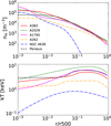 |
Fig. 1 Input radial profiles of hydrogen density nH (top panel) and temperature kT (bottom panel) for the sample selection from Table 1. These profiles were obtained by fitting the functional forms of density and temperature profiles as defined in Sects. 2.2.1 and 2.2.2 to the profiles given in Vikhlinin et al. (2006) (for galaxy clusters A383, A2029, A1795, and A262), to data from Baldi et al. (2009) (for NGC 4636), and to data from Zhuravleva et al. (2015) (for the Perseus cluster). |
2.4 Fitting procedure
The gas in galaxy clusters, groups, and massive elliptical galaxies is known to be multi-phase, and unless one fits only the high-energy part of the spectra around the Fe-K complex, single-temperature models cannot sufficiently describe the temperature structure in these objects (Buote 2000; Kaastra et al. 2004; Simionescu et al. 2009; Sanders 2023). More complex models, which are usually fitted to X-ray spectra, are either a double-temperature model or the so-called gdem model. Some earlier works preferred the wdem model instead (Kaastra et al. 2004; Werner et al. 2006; de Plaa et al. 2010). We note that the clus model accounts not only for multi-temperature but also multi-metallicity and multi-velocity structures projected along the line of sight. In our calculations, we neglected the multivelocity structure, but we took into account the presence of multiple temperatures and abundances in the 3D profiles of studied clusters.
A single-temperature model (1T) assumes the gas has just one temperature and that it is in CIE, while a double-temperature model (2T) is a superposition of two CIE models with two different temperatures. The gdem model assumes that the emission measure EM(T)3 as a function of temperature T follows a Gaussian distribution and that it can be described as
![Mathematical equation: $\[\frac{\operatorname{d~EM}(x)}{\mathrm{d} x}=\frac{\mathrm{EM}_0}{\sqrt{2 \pi} ~\sigma_x} ~\exp \left(-\frac{\left(x-x_0\right)^2}{2 \sigma_x^2}\right),\]$](/articles/aa/full_html/2025/02/aa51431-24/aa51431-24-eq20.png) (14)
(14)
where EM0 is the total integrated emission measure; x0 = log(kBT0), where T0 is the average temperature of the plasma; and σx is the width of the Gaussian distribution, which in this case is in units of x = log (kBT). To quantify the discrepancies between these three models (i.e. 1T, 2T, and gdem) and the clus model, we simulated the spectra following Sect. 2.3 and fit them with 1T, 2T, and gdem models (including the redshift and hot components). For Chandra ACIS-S, we used the 2004 response files created for the central 100 kpc of A2029 (Chandra observations ID 49774). We chose to use the response files from 2004 observations because the ACIS detectors did not suffer as much from the contamination5 at low energies (around and below 1 keV). For XRISM Resolve simulated data, we used the 20196 response files assuming 5 eV spectral resolution. For spectra simulated with Chandra ACIS-S, we ignored energies outside the 0.6–7 keV energy bins, and for XRISM Resolve, we ignored energies outside energy bins between 0.6 and 12 keV while assuming a gate valve open configuration. The data for Chandra ACIS-S CCD were simulated for an exposure time of 500 ks, while the XRISM Resolve micro-calorimeter data were simulated for an exposure time of 200 ks (except for Fig. 7, which was simulated with an exposure time of 500 ks). For all spectra in these energy ranges, we used optimal binning following Kaastra & Bleeker (2016). We evaluated the goodness of fit by using C-statistics (Cash 1979), which can be summarised as the maximum likelihood estimation in the limit of Poisson statistics. In SPEX, we used modified C-statistics based on Baker & Cousins (1984), which are described in detail in Kaastra (2017). The fit is considered good if the ΔC-statistics value of the fit is close to the expected C-statistics value. Because we do not include Poisson noise in our spectral simulations, the expected C-statistics for a model exactly matching the one used for the simulated data is identical to zero. The C-statistics of each of our fits therefore stem from the mismatches between the exact input model and the best-fit model. For the rest of this work, we denote this as ΔC-statistics.
For calculations using the 1T model, three parameters were allowed to vary: normalisation, temperature, and the iron abundance. The iron abundance is coupled to abundances from carbon to zinc. The gdem model has an additional free parameter σ, which defines the width of the Gaussian emission measure distribution (see Eq. (14); if σ = 0, the gdem model is identical to the 1T model in SPEX).
For the 2T model, we first fit the spectra with the 1T model, and only after finding the best-fit parameters of the 1T model did we add the second CIE component. The initial value for the normalisation of the second CIE component was assumed to be 10% of the best-fit normalisation of the first CIE component, and the temperature of the second CIE component was assumed to be 0.5 times the best-fit temperature of the first CIE component. We freed the temperature of the second component only if the normalisation of the second component was significant. The iron abundance of the first component was coupled to all abundances from carbon to zinc of the first component and to the abundances of the second CIE component. In the case of the 2T model, the best-fit values of temperature were then weighted by the emission measure (the normalisation of the CIE models in SPEX is equal to the emission measure). The EM weighted temperature was defined as
![Mathematical equation: $\[T_{\mathrm{EM}, \text {weighted}}=\frac{\mathrm{EM}_{\mathrm{CIE} 1} \times T_{\mathrm{CIE} 1}+\mathrm{EM}_{\mathrm{CIE} 2} \times T_{\mathrm{CIE} 2}}{\mathrm{EM}_{\mathrm{CIE} 1}+\mathrm{EM}_{\mathrm{CIE} 2}}.\]$](/articles/aa/full_html/2025/02/aa51431-24/aa51431-24-eq21.png) (15)
(15)
We calculated the error on TEM,weighted using the error propagation equation. Unless stated otherwise, all errors in this study are reported at the 1σ level. The best-fit values of the 2T model, for which the second CIE component was not significant (its normalisation was zero within the 2σ level), were removed from our sample.
3 Results
3.1 Simulations with the Chandra ACIS-S CCD
The angular resolution of Chandra allowed us to simulate spectra for the objects in Table 1 for multiple radial bins and therefore create radial profiles of the iron abundance and temperature. For all objects except NGC 4636, we defined an array of radii between 5 and 110 kpc, which are equally distributed on a logarithmic scale. Due to the low redshift as well as low mass of NGC 4636, we chose its radial bins between 0.3 and 35 kpc, which are also equally spaced on a logarithmic grid. Our results for the Perseus cluster, NGC 4636, A2029, A1795, A262, and A383 are plotted in Figs. 2, 3, B.1, B.2, B.3, and B.4, respectively. In these figures, we plot an upper limit to the expected value of C-statistics (purple dashed line in bottom left panels). The values of ΔC-statistics, which lie below the purple curve, all indicate an acceptable fit.
Figure 4 shows the results of fitting 1T, 2T, and gdem models to spectra simulated with the clus model that were extracted for the innermost and outermost radial bins (labelled in the caption). In the figure, we also plot the ratio of the best-fit values of the iron abundance and temperature to their input 3D values as defined in Eqs. (8) and (4), respectively. We evaluated the values of the 3D profiles of the iron abundance and temperature at the centres of these shells. On the x (y) axis, we plot the best-fit values to the spectra simulated without (with) RS. Deviations from the vertical line at x = 1 (along purple arrows in the bottom-right panel) indicate the magnitude of projection effects, and deviations from the diagonal line x = y (along coral arrows) indicate the magnitude of the RS effect, while deviations from the horizontal line at y = 1 (along teal arrows) indicate a combination of projection and RS effects. Due to the low count rate and large statistical uncertainties, we made the innermost and outermost shells of NGC 4636 in Fig. 4 thicker in comparison to shells chosen for the radial profiles shown in Fig. 3.
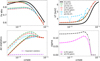 |
Fig. 2 Best-fit values of the iron abundance and temperature for spectra of the Perseus cluster simulated with Chandra ACIS-S. Spectra without RS (solid lines) and with RS (dotted lines) were fitted with 1T (green lines), 2T (blue lines), and gdem (red lines) models as described in Sect. 2.4. The top panels show the best-fit iron abundance values (top left) and best-fit temperature values (top right) together with the 3D profiles (black lines) defined in Eqs. (8) and (4), respectively. The bottom-left panel shows the values of the ΔC-statistics and the expected value of the C-statistics (purple dashed line; see Sect. 2.4 for more details). The bottom-right panel shows the best-fit value of the σ parameter, which is defined in the gdem model as the width of the Gaussian distribution of the emission measure as a function of temperature. Since the simulated data does not include the Poisson noise, the values of the ΔC-statistics that are below the purple curve indicate an acceptable fit. Spectra for every radial bin were simulated assuming an exposure time of 500 ks. |
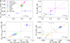 |
Fig. 4 Best-fit values of 1T (diamond points), 2T (cross), and gdem (empty circles) models to the Chandra ACIS-S simulated data with and without the effect of RS for an exposure time of 500 kiloseconds. The left panels show the best-fit iron abundance values, whereas the right panels show the best-fit values for temperature. The top and bottom panels show the best-fit values for the innermost and the outermost shells, respectively. The shell thickness for most of the objects is approximately between 5 and 6 kiloparsecs for rin and between 80 and 110 kiloparsecs for rout, with the exception of A383 (rin ∈ 5–8.5 kiloparsecs, rout ∈ 66–110 kiloparsecs) and NGC 4636 (rin ∈ 0.3–1.2 kiloparsecs, rout ∈ 12.6–35 kiloparsecs). All best-fit values have been divided by their corresponding input (3D) values. The best-fit values of the 2T model, for which the second CIE component was not significant, were removed from this plot (see last paragraph of Sect. 2.4). The 1T model results of NGC 4636 for the best-fit temperature at rout are plotted with an empty diamond point for visualisation purposes. |
3.1.1 Temperature profile
In the cores of all the studied objects, the projected temperature is higher than the input 3D temperature. For A262, A383, and Perseus, this difference is at most 10–13%, and for A2029, it is at most 20–25%. A1795 shows the largest difference out of all the studied clusters, as we observed an increase in the projected temperature by a factor of 1.5 (1T), 1.63 (gdem), and 1.8 (2T) in comparison with the input 3D temperature. The inferred temperatures are significantly higher for rin. This is expected since the 3D temperature profile as a function of radius increases towards smaller radii (before it starts decreasing in the innermost radius at approximately a few times 10−2 r500, depending on the mass of the object), and therefore there is hotter gas projected in front of and behind the inner region. However, it is worth noting that depending on the underlying profiles, some cool-core clusters are affected considerably more than others.
In the outskirts, the projected temperature is higher than its 3D value by at most 5–6% for most of the clusters. Perseus shows a slightly higher value of the projected temperature (by 7.5%). A262 and NGC 4636 (1T and gdem) show a lower projected value of the temperature in comparison with the input 3D value by at most 4%. For all the galaxy clusters studied in this paper, including or neglecting the RS effect does not make a difference when obtaining the projected temperature profiles in their cores or in their outskirts.
3.1.2 Iron abundance profile
As can be seen in the top-left panel of Fig. 4, the iron abundance of most of the clusters in our sample can be lower or higher by 5–10% in their cores due to the projection effects, with the exception of 1T and gdem fits to the A1795 spectrum, which show higher values by approximately 10–20% due to the projection effects. After fitting 1T, 2T, and gdem models to the simulated spectra of the Perseus cluster, A2029, and A383, we noticed similar behaviour of the best-fit iron abundance profiles in their cores. The projected iron abundance profiles show a clear separation between data simulated with and without RS. If constrained, all three models (1T, 2T, and gdem) predict lower iron abundance values in the cores of these clusters if the RS is present in their simulated spectra. Contrary to the results for the Perseus cluster, A2029, and A383, the projected profiles of the iron abundance in the cores of A1795 and A262 do not show such differences between fitting the data simulated with or without RS. The ΔC-statistics values are worse if RS is taken into account. This result is not surprising since the RS is not included in 1T, 2T, nor gdem models.
In the outskirts, the projected iron abundance of the more massive galaxy clusters (A2029, A1795, A383, and the Perseus cluster) in our sample is lower by approximately 10% due to the projection effects, while for the less massive object A262, this difference between the projected value and the input iron abundance value rises to approximately 14–20%. The projected values of iron abundance in the outskirts of all clusters in our sample are lower than their 3D input profiles.
3.1.3 NGC 4636
The differences between the 2D and 3D iron abundance and temperature profiles in the core (rin ∈ 0.3–1.2 kpc) and outskirts (rout ∈ 12.6–35 kpc) of NGC 4636 are shown in Fig. 4. The best-fit projected temperature in the core of NGC 4636 is higher by a factor of around 1.5 for 1T and 2T models, while the gdem model shows a smaller difference between 2D and 3D temperatures (an increase by approximately 10%). This difference is caused by the projection effects. In the outskirts, the projected temperature is lower by 3.5% for the 1T and gdem model, while the 2T model is statistically not significant. The effect of RS on the inferred temperature profile is the largest in the core and in the case of the gdem (increase by approximately 18%) and 2T models (decrease by approximately 17%), and it is the smallest in the case of the 1T model (increase by ~6%). In the outskirts, the effect of RS on the projected temperature is within <2%.
The massive elliptical galaxy NGC 4636 shows the biggest differences in the recovered shape of the iron abundance profile. Out of all the considered objects in this paper, this is the only case where we can reproduce a drop in the iron abundance profile in the few innermost kiloparsecs, which has been observed with XMM-Newton (see Sect. 4 for more details). Due to projection, the iron abundance in the core drops by ≈80% (1T) and ≈30% (2T). In the case of fitting its simulated spectra with the gdem model, we noticed an increase in the projected value of iron abundance by ≈20% in comparison with the input iron abundance value. For the 1T model, there is almost no difference between the best-fit iron abundance values with and without RS. On the other hand, if RS is present in the simulated data, the iron abundance inferred from fitting 2T and gdem models to simulated spectra shows a decrease by approximately 50 and 58%, respectively.
3.1.4 Comparison of the input and fitted emission measure distributions
In Fig. 5 we plot the input emission measure as a function of temperature for the Perseus cluster (left panels) and NGC 4636 (right panels), and we compare it to the Gaussian distribution retrieved from the best-fit gdem model following Eq. (14). The histograms in Fig. 5 were created by taking cylindrical cuts through the cluster for different radii (representing 2D/projected shells of the cluster). For each 3D radius within this cylinder, the 3D density and 3D temperature were calculated using the radial profiles defined in Sects. 2.2.1 and 2.2.2. This allowed us to obtain EM in each of these infinitesimally small integration volumes. We then calculated the distribution of EM as a function of temperature in each of these 2 D shells and plotted the results with histogram bars. The width of the temperature bins was assumed to be the same as the underlying EM distribution of the best-fit gdem model. We inspected two 2D shells while making sure that in one of these 2D shells the sigma parameter reached its maximum (see the bottom-right panel in Figs. 2 and 3).
Our results show that for both targets, the gdem model does not accurately represent the shape of the input EM. The smallest difference between the best-fit gdem model and the input EM distribution is for the shells with σ ≈ 0.14 (Perseus) and σ ≈ 0.2 (NGC 4636). Even in this case one might argue that the gdem model might not represent the input EM distribution of these shells most accurately and that a decreasing power law or a skewed gdem model would be preferred.
In the innermost projected shell of the Perseus cluster, the input EM is skewed towards a single temperature whose value coincides with the 3 D value in its core (≈3.3 keV). Both best-fit gdem models (with and without RS) overestimate the amount of gas with temperatures below and above this peak temperature.
In the case of NGC 4636, the best-fit gdem model (no RS) peaks at a slightly different temperature in comparison with the input EM distribution, which results in overestimating the amount of gas with temperatures below 0.1 keV and underestimating the gas at higher temperatures. The tail of the EM distribution of this massive elliptical galaxy (above 0.4 keV) agrees well with the gdem results (no RS). In the case of the best-fit gdem values including RS, the gdem model peaks at the same temperature as the input EM distribution; however, it overestimates the amount of gas with temperatures lower or higher that this peak. The tail of this gdem best-fit distribution agrees well with the input EM distribution for temperatures above ≈0.6 keV. Again, the input EM distribution could be described more accurately by a different model, such as the skewed gdem model.
In the outskirts of both objects, the best-fit gdem values of σ were either identical with zero or very close to zero. We stress that the plotted histograms in Fig. 5 only take into account the effect of projection. When we refer to the gas as being multiphase, we mean considering its 3D temperature profile as defined in Fig. 1, and we neglect other effects that can also change the phase of the gas (e.g. cooling instabilities).
3.2 Simulations with the XRISM Resolve micro-calorimeter
The design of the XRISM Resolve micro-calorimeter in combination with its 3′ × 3′ field of view and the angular resolution of 1.7 arcminutes limited our simulations to only two radial bins. From these bins, we extracted the spectra of the studied objects:
rin = 0–0.75′, which corresponds to a 1.5′ × 1.5′ array, and
rout = 0.75′−1.5′, which corresponds to the rest of the 3′ × 3′ array.
In Fig. 6, we show the results of fitting the 1T, 2T, and gdem models to simulated spectra extracted for the inner and outer radial bins as defined in the figure caption. In the figure, we plot the best-fit values of the iron abundance and temperature for two cases, namely with and without the effect of RS. The values of 3D profiles of the iron abundance and temperature are evaluated at the centres of these shells following Eqs. (8) and (4), respectively. Our simulations were done assuming the response files for an open gate valve; however, at the moment the gate valve opening attempts have not been successful. In the event that the gate valve remains closed for an extended period of time, we plan to redo our simulations in the future with the updated response files.
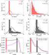 |
Fig. 5 Emission measure distribution as a function of temperature for the Perseus cluster (left panels) and NGC 4636 (right panels). The different colours represent different shells that were used to extract the input emission measure distribution as described in Sect. 3.1.4 (plotted with histograms). The Gaussian functions in each plot were obtained following Eq. (14) and by using the best-fit values obtained and described in more details in Sect. 3.1. The bottom row shows the radial profile of best-fit values of σ for the Perseus cluster and NGC 4636, where the red and black bars correspond to radial bins used for deriving the EM distribution in the first two rows of this figure. |
3.2.1 Temperature profile
In the inner shells, the differences between the 3D temperatures and the best-fit projected values are slightly larger in comparison with the outer shells due to the same reason we discussed in Sect.3.1.1. As shown in Fig. 6, the best-fit values for rin are larger by at most 6% (Perseus) to 26% (A1795, 2T), with the exception of A383, for which the best-fit temperature is lower by 2% in comparison with the input temperature. In the outer shells, the best-fit values are higher at most by ~3% (A2029, 1T) to 23% (Perseus, 2T) for most of the studied objects. For A383, the 2D temperature is lower by ~6%. For all objects besides A383, the best-fit temperatures are always higher than the input 3D temperatures for both inner and outer shells.
From Fig. 6, one can see that the presence or absence of RS in the spectra of almost all objects considered in this study does not affect the projected temperature (within error bars) recovered from fitting the simulated spectra with models such as 1T, 2T, or gdem (the data points lie on the diagonal solid black line). This is true for both of the radial bins (rin and rout). The only exception is the 2T fit in the outer radial bin of the Perseus cluster, where the projected temperature increased by approximately 7% due to the presence of RS in the simulated data.
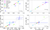 |
Fig. 6 Same as Fig. 4 but for data simulated with the XRISM Resolve micro-calorimeter. The exposure time was assumed to be 200 kiloseconds. The physical sizes of inner shells are approximately (0–3) kiloparsecs for NGC 4636, (0–16) kiloparsecs for Perseus and A262, (0–54) kiloparsecs for A1795, (0–66) kiloparsecs for A2029, and (0–142) kiloparsecs for A383. The physical sizes of outer shells are approximately (3–7) kiloparsecs for NGC 4636, (16–33) kiloparsecs for Perseus and A262, (54–108) kiloparsecs for A1795, (66–133) kiloparsecs for A2029, and (142–283) kiloparsecs for A383. The errors represent the standard deviation 1σ. Similar to Fig. 4, the best-fit values of the 2T model, for which the second CIE component was not significant, were removed from this plot (see the last paragraph of Sect. 2.4). The 1T model results of A383 for the best-fit temperature in both radial bins are plotted with an empty diamond point for visualisation purposes. |
3.2.2 Iron abundance profile
Compared to Chandra simulations, XRISM simulations yield slightly higher values for the effect of projection, as well as RS, on the iron abundance in the inner shell of galaxy clusters. The projection effects make the iron abundance in the cores of the galaxy clusters lower by ~1–20% when compared to the input 3D values. These effects are the lowest (~1–5%) for the Perseus cluster, A383, and A262 (the gdem model). For A2029, A1795, and A262 (1T), the projection effects make the iron abundance in the core of these clusters lower by approximately 8–20% in comparison with the input abundance. In the outer shells, the projection effects make the inferred iron abundance lower by 13–20%, with the exception of the Perseus cluster, for which we observed an effect of approximately 6–8%.
The effect of the RS on the inferred iron abundance is slightly higher in the cores of galaxy clusters in comparison with their outskirts; however, for all the clusters studied in this paper, we observed a maximum effect of 10% in both of the radial bins. Fitting 1T, 2T, and gdem models to spectra simulated with RS causes a decrease in the projected iron abundance for all clusters from our sample except the outskirts of A383. The largest effect of RS occurred in the case of the Perseus cluster (~11% in the core and ~8% in the outer shell). We summarise these results (together with NGC 4636, which is discussed in a separate section) in Table 2.
3.2.3 NGC 4636
The temperature in the core of NGC 4636 inferred from the gdem model is affected the least by the projection (~10%), while in the case of 1T and 2T models, this value rises to ~24%. In the outskirts, all three models yield similar results, and the projection effects cause an increase in temperature by at most 10% in comparison with the 3D values. In both radial bins, the RS does not significantly affect the projected temperature obtained from the 1T, 2T, and gdem models.
Similar to our conclusions in Sect. 3.1, the best-fit values of the iron abundance in the core of NGC 4636 are affected the most by fitting the 1T, 2T, and gdem models to the spectra simulated with the clus model. The projection effects make the iron abundance in the core lower by 55 and 15% for the 1T and 2T models, respectively. In the case of the gdem model, the projected iron abundance is higher by 5% in comparison with the input 3D profile. If the RS is taken into account in the simulated spectrum, the iron abundance decreases by approximately 10 (1T), 17 (2T), and 22% (gdem). In the outskirts, the 1T model shows the largest sensitivity to the projection effects, while the gdem model shows the largest sensitivity if RS is taken into account. Both of these effects are below 10%.
In Fig. 7, we show NGC 4636 simulated spectra (with RS) for a shell from 0.3 to 7 kpc (full field of view) for a 500 ks XRISM/Resolve observation. In the figure, we compare data simulated with the clus model (black points) to the best-fit 1T (blue solid line), 2T (green solid line), and gdem (red solid line) models. We plot the residuals between the simulated data and the 1T, 2T, and gdem models in the bottom three panels. These residuals show that the 1T, 2T, and gdem models cannot fully describe the richness of the NGC 4636 spectra, especially if the resolution of the observed spectrum is similar to XRISM Resolve. Additionally, the discrepancy between 2D and 3D profiles for XRISM simulated data is slightly lower in comparison with simulations for Chandra, which is mostly due to the difference in their spatial resolution.
4 Discussion
4.1 Multi-temperature and multi-metallicity structure of the ICM
Our results show that even if the temperature and gas density distribution is smooth and the gas is isothermal at every shell while no thermal instabilities are present in the ICM, the projection effects influence the best-fit temperatures obtained from fitting the complex spectra of galaxy clusters and NGC 4636 with models such as 1T, 2T, and gdem. In Fig. 4, we show that in the cores of some cool-core clusters, the projected temperature is within 8–12% of the input temperature (e.g. see the core of A262), while in other cool-core clusters, for example the core of A1795, the projection effects caused a difference between the input temperature and the projected temperature as large as a factor of 1.5–1.8. In the case of the core of NGC 4636 (1T and 2T models), this factor is 1.5, while the temperature inferred from the gdem model is 10% higher in comparison to the input value. For all objects studied in this paper, the 2D temperature is higher in comparison with the 3D input temperature.
Compared to the Chandra simulations, the temperature in the inner radius inferred from the XRISM simulations is less affected by the projection effects (for most of the clusters; see Fig. 6). On the other hand, the temperature inferred from the XRISM simulations in rout is affected slightly more by projection compared to the temperature inferred from the Chandra simulations.
It is well known that the 1T model cannot describe the multi-temperature structure of galaxy clusters accurately and that it leads to an ‘iron bias’ (Buote 2000) for the low-temperature objects and to an ‘inverse iron bias’ for the high-temperature objects (Rasia et al. 2008; Simionescu et al. 2009; Gastaldello et al. 2010). Simionescu et al. (2009) concluded that for the cool-core cluster Hydra A, one needs a broad emission measure distribution, such as the gdem model, to simultaneously fit the lines of the Fe-K and Fe-L complexes, which indicate a multi-temperature origin of the gas. Kaastra et al. (2004) concluded that, in most cases, the 2T model can sufficiently describe the spectra of cool-core clusters. However, as our results show, in many cases neither the 2T nor the gdem model can accurately describe the underlying emission measure distribution, as shown in Fig. 5, even when the fit is statistically acceptable (see all values of ΔC-statistics that lie below the purple dashed curve in the bottom-left panels of Figs. 3, B.1, B.2, B.3, and B.4). This shows the difficulty of reconstructing the input temperature profile from the projected values, even for a smooth temperature profile assuming a set of isothermal shells and neglecting any cooling instabilities. Such findings might impact the cross-calibration studies involving different instruments, which in return might affect the inferred masses of galaxy clusters and therefore also the cosmological parameters (e.g. see Wallbank et al. 2022; Migkas et al. 2024).
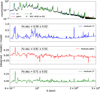 |
Fig. 7 XRISM Resolve spectra in the energy range 0.6–3 keV simulated with the clus model (including RS) for the 0.3–7 kpc aperture region of NGC 4636 (black points) while assuming the gate valve is open. The best-fit 1T, 2T, and gdem models are plotted with blue, green, and red solid lines together with the residuals that are shown in bottom three panels. The best-fit values of the iron abundance are given in the plots together with 1σ errors. The exposure time was assumed to be 500 ks. |
4.2 Measured Fe abundance drop in the cores
As already mentioned in the introduction of this paper, some galaxy clusters, galaxy groups, and massive elliptical galaxies show a sharp decrease in the radial profiles of the metal content in their innermost few kiloparsecs. A unified theory explaining the reason behind this abundance drop has not yet been established. In this paper, we investigated whether projection effects and the RS process can potentially explain the measured abundance profiles in some of these objects.
Out of the objects studied in this paper, only the cores of the Perseus cluster and the massive elliptical galaxy NGC 4636 have a confirmed abundance drop in their projected profiles, such as in the XMM-Newton observations (Werner et al. 2009 for NGC 4636 and Mernier et al. 2017 for NGC 4636 and the Perseus cluster). We compared our results to the work of Mernier et al. (2017) since the authors used the same set of proto-solar abundances by Lodders et al. (2009). The iron abundance was measured by fitting gdem to the XMM-Newton data, resulting in a decrease from 0.9 ZFe/ZFe,⊙ at ~0.02 r500 to 0.5 ZFe/ZFe,⊙ at ~0.003 r500 for NGC 4636, while for the Perseus cluster the iron abundance drops from 0.8 ZFe/ZFe,⊙ at ~0.03 r500 to 0.6 ZFe/ZFe,⊙ at ~0.004 r500. The authors find no abundance drop in A2029 nor in A1795, while A262 shows a sharp increase from 0.6 ZFe/ZFe,⊙ at ~0.1 r500 to 1.4 ZFe/ZFe,⊙ at ~0.007 r500. Similar conclusions of no significant abundance drop in the few innermost kiloparsecs were reached for A2029 with Chandra ACIS-S observations (Fig. 4 of Lewis et al. 2002), for A1795 with XMM-Newton observations (Fig. 1 of Tamura et al. 2001) and with Chandra ACIS observations (Fig. 7 of Ettori et al. 2002), and for A262 with Suzaku observations (Fig. 3 of Sato et al. 2009). Besides a global abundance value reported for A383 in Morandi et al. (2010), which reaches 0.52 ± 0.07 of the solar value for Grevesse & Sauval (1998) abundances, we could not find the radial profile of the iron abundance in currently existing literature.
A few previous works such as Rasmussen & Ponman (2007) and Russell et al. (2008) concluded that projection effects do not significantly impact the measured iron abundance profiles. Depending on the mass of the simulated objects as well as the projected distance from the core, we find different conclusions based on our simulations.
4.2.1 Perseus
For the core of the Perseus cluster, Churazov et al. (2004) and Gastaldello & Molendi (2004) concluded that there is no evidence for RS based on XMM-Newton data. However, measurements with the Hitomi SXS micro-calorimeter showed that the RS suppresses the flux measured in the Fe XXV Heα line by a factor of ~1.3 in the inner ~30 kpc (Hitomi Collaboration 2018b). From our simulations with Chandra ACIS-S as well as XRISM Resolve, we can conclude that
the projection effects cannot explain the abundance drop in the core of the Perseus cluster and that all the used models (1T, 2T, and gdem) cause an increase (decrease) in the iron abundance at most by 5% based on simulations with Chandra (XRISM).
the effect of RS can only partly explain the iron abundance drop in the core of Perseus, and according to our results, the measured iron abundance can maximally decrease by 10–15%.
Similar conclusions were reported in Sanders & Fabian (2006), who showed that RS cannot remove the central drop in the Chandra CCD spectra of galaxy clusters (namely Centaurus and A2199) and that this effect can change the measured metallicities at most by 10%. These results are in agreement with our studies. Additionally, the Perseus cluster is not a perfectly symmetric system, and faint X-ray cavities as well as weak shocks, ripples, and radio lobes around its central galaxy NGC 1275 are present in its ICM (e.g. see McNamara et al. 1996; Fabian et al. 2011; Hitomi Collaboration 2018a). Such effects are, however, neglected in our simulations. We defer simulations of non-spherically symmetric systems as well as of additional clusters known to host abundance dips to future work.
4.2.2 NGC 4636
The massive elliptical galaxy NGC 4636 is known for showing RS in its core, which changes the flux ratio between the resonant line at 15.01 Å and forbidden lines at 17.05 and 17.10 Å of Fe XVII (Xu et al. 2002; Kahn et al. 2003; Hayashi et al. 2009; Werner et al. 2009; Ahoranta et al. 2016). As we have mentioned earlier in this paper, it also has a steep abundance drop measured in its core, which makes it a perfect candidate to test the theory of whether accounting for the RS effect can remove this central abundance drop.
NGC 4636 was one of the five massive elliptical galaxies studied in Werner et al. (2009). The authors fitted the observed spectra with a 1T model and concluded that more complicated models did not improve the fit and that differential emission measure models always converged to the single-temperature approximation. This is not in agreement with our findings presented in Fig. 5, which shows that in the core, the differential emission measure should follow a decreasing power law or perhaps a skewed gdem model.
Depending on the model (1T, 2T, or gdem) used to fit the simulated data of NGC 4636, we confirm that the central abundance drop in this massive elliptical galaxy can potentially be explained by the RS and, in the case of the 1T model, also solely by projection effects. The models 1T, 2T, and gdem, neglect the RS effect, which influences the measurement of fluxes in Fe XVII lines. Our results indicate larger differences between 3D and projected values (50–58%, depending on the model) in comparison with those reported in Werner et al. (2009), where the authors concluded that the RS can lead to underestimation of Fe and O abundances by 10–20% in its core.
As previously mentioned, in Mernier et al. (2017) the iron abundance measured using the gdem model drops from 0.9 ZFe/ZFe,⊙ at ~0.02 r500 to 0.5 ZFe/ZFe,⊙ at ~0.003 r500. Using the same model as the authors (gdem) to fit the spectra, we performed the simulation with the clus model while taking into account the RS. We report a drop approximately from 0.86 ZFe/ZFe,⊙ at ~0.02 r500 to 0.33 ZFe/ZFe,⊙ at ~0.003 r500. These findings are in agreement with observations by Mernier et al. (2017) (within statistical uncertainties).
Similar to our discussion of the results for the Perseus cluster, we point out that NGC 4636 is known for its non-spherical nature. Its X-ray images show a presence of X-ray bubbles and cavities as well as spiral arms, which are believed to originate from shocks caused by the central AGN and its interaction with the surrounding ICM (e.g. see Jones et al. 2002; Baldi et al. 2009). The clus model assumes a spherical symmetry when simulating X-ray spectra. This assumption breaks down for NGC 4636, and it might affect the results reported in this paper. However, we do not expect that the central abundance drop for this object would completely disappear.
5 Conclusions
This paper introduces the clus model, which was recently implemented in the software package SPEX. The clus model can be used for any X-ray emitting plasma that is in CIE and that can be approximated with spherical symmetry. The advantage of this model lies in the forward modelling of spectra and radial profiles of selected sources, assuming their 3D temperature, density, velocity, and metal abundance profiles. The X-ray emitting gas is divided into a set of spherically symmetric shells where the emission in each shell is described with a single CIE model and projected onto the sky. This model also includes the RS effect, which is implemented through Monte Carlo simulations.
We used the clus model to simulate spectra of galaxy clusters Abell 383, Abell 2029, Abell 1795, and Abell 262; the Perseus cluster; and the massive elliptical galaxy NGC 4636. We modelled spectra of these objects with and without RS while assuming CCD-like (Chandra ACIS-S) and microcalorimeter (XRISM Resolve) spectral resolutions. We created projected radial profiles of their metal abundance and temperature by fitting their simulated spectra with single-temperature (1T), double-temperature (2T), and Gaussian-shaped differential emission measure (gdem) models.
As we have shown in this paper, the impact of projection and RS effects varies depending on the mass or temperature of the object as well as the projected distance from its core. Our main conclusions are summarised as follows:
As shown by the differential emission measure for the Perseus cluster and NGC 4636 (see Fig. 5), the 1T, 2T, and gdem models do not always accurately describe the underlying EM distribution. The EM distribution changes depending on the projected distance from the cluster core as well as the thickness of the shell. Depending on these properties, different models, such as a skewed gdem model or decreasing power law, might be more suitable to describe the EM profile. Hence, fitting data with a model that does not represent the underlying distribution can lead to fitting biases.
The projection effects cause an increase of temperature inferred from fitting 1T, 2T, or gdem models to the simulated spectra in the cores of studied objects, with the exception of XRISM simulations for A383. For clusters with a less prominent core in their density profile, this increase is 10–30% (6–18%) for Chandra (XRISM), while for the objects with a more prominent core in the density profile, such as A1795 and NGC 4636, this increase can be as high as a factor of 1.5–1.8 if spectra were simulated with Chandra. For XRISM simulations, these factors are slightly lower ~(1.2–1.26) due to a lower spatial resolution. In the outskirts of galaxy clusters, the differences are below 8% for Chandra; however, XRISM simulations show that the projected temperature can be higher by 3–23% in comparison with its input value.
Using models such as the clus model for fitting CCD and micro-calorimeter spectra is more crucial for obtaining the abundance profiles of low-mass and low-temperature objects (see Figs. 4 and 6). In the outskirts of A262, the projected iron abundance is 14–20% lower than the input profile irrespective of the model used for fitting its simulated spectra. In the core of the massive elliptical galaxy NGC 4636, the projected iron abundance is lower by almost 80% (55%) for the 1T model and higher by 20% (5%) for the gdem model if spectra were simulated with Chandra (XRISM). Regardless of the instrument, the gdem model is affected the least by the projection effects in the core of NGC 4636. However, we report non-negligible differences between the input and projected profiles also for hotter and more massive objects. For some cool-core clusters, the differences might be negligible (e.g. iron abundance in the core of A383 simulated with Chandra and XRISM), while in other cool-core clusters, for example A1795, the projected iron abundance in its core is approximately 20% higher (lower) in comparison with the input profile if data were simulated with Chandra (XRISM).
The RS can reduce the observed central abundance drop in galaxy clusters such as the Perseus cluster by at most 10–15%, but it cannot fully explain the abundance drop in the few innermost kiloparsecs. Similar conclusions were reported in Sanders & Fabian (2006) for the Centaurus and A2199 galaxy clusters.
In the case of the massive elliptical galaxy NGC 4636, the RS can potentially explain the abundance drop measured in its core. Depending on the model used for fitting its spectra, not accounting for the RS leads to an underestimation of the iron abundance in the core of this massive elliptical galaxy by ~50% (2T) to 58% (gdem) if data were simulated with Chandra. In the case of the 1T model, this abundance drop can also be solely explained by projection effects. The XRISM simulations show that RS can make the iron abundance in the core of NGC 4636 lower by at most 10–22%. Our results indicate larger differences between 3D and projected values (50–58% depending on the model) in comparison with those reported in Werner et al. (2009), where the authors concluded that RS can lead to underestimation of Fe and O abundances by 10–20% in its core.
In conclusion, our results show that depending on the mass of the object as well as the projected distance from its core, neither a single-temperature or double-temperature model nor the Gaussian-shaped differential emission measure model can accurately describe the input emission measure distribution of these massive objects. Additionally, we showed that depending on the underlying thermodynamic profiles of galaxy clusters, galaxy groups, and massive elliptical galaxies, the projection effects and the effect of resonant scattering can potentially explain the observed dip in the iron abundance profile in the cores of some of these objects. More specifically, we were able to reproduce such a behaviour for NGC 4636. However, in the more massive objects, for example galaxy clusters, these effects were not large enough to explain the observed lack of metals in their cores.
Data availability
The dataset generated and analysed during this study is available at https://doi.org/10.5281/zenodo.14652473.
Acknowledgements
The authors acknowledge the financial support from NOVA, the Netherlands Research School for Astronomy. A.S. acknowledges the Kavli IPMU for the continued hospitality. SRON Netherlands Institute for Space Research is supported financially by NWO. L.S. acknowledges the financial support of the GAČR EXPRO grant No. 21-13491X.
Appendix A Additional material
In Table A.1 we provide a complete set of all clus parameters. The acronyms of the parameters are their names as used in the SPEX interface and all variables are described in Sec. 2.2.
Complete set of 80 parameters of the clus model.
Appendix B Chandra simulations for other clusters
References
- Ahoranta, J., Finoguenov, A., Pinto, C., et al. 2016, A&A, 592, A145 [NASA ADS] [CrossRef] [EDP Sciences] [Google Scholar]
- Baker, S., & Cousins, R. D. 1984, Nucl. Instrum. Methods Phys. Res., 221, 437 [Google Scholar]
- Baldi, A., Forman, W., Jones, C., et al. 2009, ApJ, 707, 1034 [Google Scholar]
- Böhringer, H., & Werner, N. 2010, A&A Rev., 18, 127 [CrossRef] [Google Scholar]
- Buote, D. A. 2000, MNRAS, 311, 176 [Google Scholar]
- Cash, W. 1979, ApJ, 228, 939 [Google Scholar]
- Cavaliere, A., & Fusco-Femiano, R. 1976, A&A, 49, 137 [NASA ADS] [Google Scholar]
- Churazov, E., Forman, W., Jones, C., & Böhringer, H. 2003, ApJ, 590, 225 [NASA ADS] [CrossRef] [Google Scholar]
- Churazov, E., Forman, W., Jones, C., Sunyaev, R., & Böhringer, H. 2004, MNRAS, 347, 29 [NASA ADS] [CrossRef] [Google Scholar]
- de Plaa, J., Werner, N., Simionescu, A., et al. 2010, A&A, 523, A81 [NASA ADS] [CrossRef] [EDP Sciences] [Google Scholar]
- de Plaa, J., Zhuravleva, I., Werner, N., et al. 2012, A&A, 539, A34 [NASA ADS] [CrossRef] [EDP Sciences] [Google Scholar]
- Ettori, S., & Fabian, A. C. 2006, MNRAS, 369, L42 [NASA ADS] [CrossRef] [Google Scholar]
- Ettori, S., Fabian, A. C., Allen, S. W., & Johnstone, R. M. 2002, MNRAS, 331, 635 [Google Scholar]
- Fabian, A. C., Sanders, J. S., Allen, S. W., et al. 2011, MNRAS, 418, 2154 [Google Scholar]
- Forman, W., Kellogg, E., Gursky, H., Tananbaum, H., & Giacconi, R. 1972, ApJ, 178, 309 [Google Scholar]
- Fukushima, K., Kobayashi, S. B., & Matsushita, K. 2022, MNRAS, 514, 4222 [NASA ADS] [CrossRef] [Google Scholar]
- Gastaldello, F., & Molendi, S. 2004, ApJ, 600, 670 [Google Scholar]
- Gastaldello, F., Ettori, S., Balestra, I., et al. 2010, A&A, 522, A34 [NASA ADS] [CrossRef] [EDP Sciences] [Google Scholar]
- Gilfanov, M. R., Syunyaev, R. A., & Churazov, E. M. 1987, Sov. Astron. Lett., 13, 3 [NASA ADS] [Google Scholar]
- Grevesse, N., & Sauval, A. J. 1998, Space Sci. Rev., 85, 161 [Google Scholar]
- Gu, L., Zhuravleva, I., Churazov, E., et al. 2018, Space Sci. Rev., 214, 108 [Google Scholar]
- Hayashi, K., Fukazawa, Y., Tozuka, M., et al. 2009, PASJ, 61, 1185 [NASA ADS] [Google Scholar]
- Hitomi Collaboration (Aharonian, F., et al.) 2018a, PASJ, 70, 9 [NASA ADS] [Google Scholar]
- Hitomi Collaboration (Aharonian, F., et al.) 2018b, PASJ, 70, 10 [NASA ADS] [Google Scholar]
- Johnstone, R. M., Allen, S. W., Fabian, A. C., & Sanders, J. S. 2002, MNRAS, 336, 299 [NASA ADS] [CrossRef] [Google Scholar]
- Jones, C., Forman, W., Vikhlinin, A., et al. 2002, ApJ, 567, L115 [Google Scholar]
- Kaastra, J. S. 2017, A&A, 605, A51 [NASA ADS] [CrossRef] [EDP Sciences] [Google Scholar]
- Kaastra, J. S., & Bleeker, J. A. M. 2016, A&A, 587, A151 [NASA ADS] [CrossRef] [EDP Sciences] [Google Scholar]
- Kaastra, J. S., Mewe, R., & Nieuwenhuijzen, H. 1996, in UV and X-ray Spectroscopy of Astrophysical and Laboratory Plasmas, eds. K. Yamashita, & T. Watanabe (Japan: Academic Press), 411 [Google Scholar]
- Kaastra, J. S., Tamura, T., Peterson, J. R., et al. 2004, A&A, 413, 415 [NASA ADS] [CrossRef] [EDP Sciences] [Google Scholar]
- Kaastra, J. S., Paerels, F. B. S., Durret, F., Schindler, S., & Richter, P. 2008, Space Sci. Rev., 134, 155 [Google Scholar]
- Kaastra, J. S., Raassen, A. J. J., de Plaa, J., & Gu, L. 2018, https://doi.org/10.5281/zenodo.2419563 [Google Scholar]
- Kaastra, J. S., Raassen, A. J. J., de Plaa, J., & Gu, L. 2020, https://doi.org/10.5281/zenodo.4384188 [Google Scholar]
- Kahn, S. M., Peterson, J. R., Paerels, F. B. S., et al. 2003, ASP Conf. Ser., 301, 23 [NASA ADS] [Google Scholar]
- Kellogg, E., Gursky, H., Tananbaum, H., Giacconi, R., & Pounds, K. 1972, ApJ, 174, L65 [NASA ADS] [CrossRef] [Google Scholar]
- Lakhchaura, K., Mernier, F., & Werner, N. 2019, A&A, 623, A17 [NASA ADS] [CrossRef] [EDP Sciences] [Google Scholar]
- Lewis, A. D., Stocke, J. T., & Buote, D. A. 2002, ApJ, 573, L13 [Google Scholar]
- Liu, A., Zhai, M., & Tozzi, P. 2019, MNRAS, 485, 1651 [NASA ADS] [CrossRef] [Google Scholar]
- Lodders, K., Palme, H., & Gail, H. P. 2009, Landolt-Börnstein (Berlin: Springer), 4B, 712 [Google Scholar]
- McNamara, B. R., O’Connell, R. W., & Sarazin, C. L. 1996, AJ, 112, 91 [NASA ADS] [CrossRef] [Google Scholar]
- Mernier, F., de Plaa, J., Kaastra, J. S., et al. 2017, A&A, 603, A80 [NASA ADS] [CrossRef] [EDP Sciences] [Google Scholar]
- Migkas, K., Kox, D., Schellenberger, G., et al. 2024, A&A, 688, A107 [NASA ADS] [CrossRef] [EDP Sciences] [Google Scholar]
- Million, E. T., Allen, S. W., Werner, N., & Taylor, G. B. 2010, MNRAS, 405, 1624 [NASA ADS] [Google Scholar]
- Mohr, J. J., Mathiesen, B., & Evrard, A. E. 1999, ApJ, 517, 627 [Google Scholar]
- Morandi, A., Pedersen, K., & Limousin, M. 2010, ApJ, 713, 491 [NASA ADS] [CrossRef] [Google Scholar]
- Nelson, D., Byrohl, C., Ogorzalek, A., et al. 2023, MNRAS, 522, 3665 [NASA ADS] [CrossRef] [Google Scholar]
- Ogorzalek, A., Zhuravleva, I., Allen, S. W., et al. 2017, MNRAS, 472, 1659 [NASA ADS] [CrossRef] [Google Scholar]
- Panagoulia, E. K., Fabian, A. C., & Sanders, J. S. 2013, MNRAS, 433, 3290 [NASA ADS] [CrossRef] [Google Scholar]
- Panagoulia, E. K., Sanders, J. S., & Fabian, A. C. 2015, MNRAS, 447, 417 [CrossRef] [Google Scholar]
- Pinto, C., Sanders, J. S., Werner, N., et al. 2015, A&A, 575, A38 [NASA ADS] [CrossRef] [EDP Sciences] [Google Scholar]
- Rafferty, D. A., Bîrzan, L., Nulsen, P. E. J., et al. 2013, MNRAS, 428, 58 [CrossRef] [Google Scholar]
- Rasia, E., Mazzotta, P., Bourdin, H., et al. 2008, ApJ, 674, 728 [Google Scholar]
- Rasmussen, J., & Ponman, T. J. 2007, MNRAS, 380, 1554 [CrossRef] [Google Scholar]
- Russell, H. R., Sanders, J. S., & Fabian, A. C. 2008, MNRAS, 390, 1207 [NASA ADS] [CrossRef] [Google Scholar]
- Sanders, J. S. 2023, arXiv e-prints [arXiv:2301.12791] [Google Scholar]
- Sanders, J. S., & Fabian, A. C. 2002, MNRAS, 331, 273 [NASA ADS] [CrossRef] [Google Scholar]
- Sanders, J. S., & Fabian, A. C. 2006, MNRAS, 370, 63 [NASA ADS] [CrossRef] [Google Scholar]
- Sanders, J. S., & Fabian, A. C. 2007, MNRAS, 381, 1381 [Google Scholar]
- Sato, K., Matsushita, K., & Gastaldello, F. 2009, PASJ, 61, S365 [NASA ADS] [CrossRef] [Google Scholar]
- Schindler, S., Kapferer, W., Domainko, W., et al. 2005, A&A, 435, L25 [NASA ADS] [CrossRef] [EDP Sciences] [Google Scholar]
- Simionescu, A., Werner, N., Finoguenov, A., Böhringer, H., & Brüggen, M. 2008, A&A, 482, 97 [NASA ADS] [CrossRef] [EDP Sciences] [Google Scholar]
- Simionescu, A., Werner, N., Böhringer, H., et al. 2009, A&A, 493, 409 [NASA ADS] [CrossRef] [EDP Sciences] [Google Scholar]
- Tamura, T., Kaastra, J. S., Peterson, J. R., et al. 2001, A&A, 365, L87 [NASA ADS] [CrossRef] [EDP Sciences] [Google Scholar]
- Vikhlinin, A., Kravtsov, A., Forman, W., et al. 2006, ApJ, 640, 691 [Google Scholar]
- Wallbank, A. N., Maughan, B. J., Gastaldello, F., Potter, C., & Wik, D. R. 2022, MNRAS, 517, 5594 [NASA ADS] [CrossRef] [Google Scholar]
- Werner, N., de Plaa, J., Kaastra, J. S., et al. 2006, A&A, 449, 475 [NASA ADS] [CrossRef] [EDP Sciences] [Google Scholar]
- Werner, N., Zhuravleva, I., Churazov, E., et al. 2009, MNRAS, 398, 23 [NASA ADS] [CrossRef] [Google Scholar]
- Willingale, R., Starling, R. L. C., Beardmore, A. P., Tanvir, N. R., & O’Brien, P. T. 2013, MNRAS, 431, 394 [Google Scholar]
- Xu, H., Kahn, S. M., Peterson, J. R., et al. 2002, ApJ, 579, 600 [NASA ADS] [CrossRef] [Google Scholar]
- Zhuravleva, I., Churazov, E., Sunyaev, R., et al. 2013, MNRAS, 435, 3111 [NASA ADS] [CrossRef] [Google Scholar]
- Zhuravleva, I., Churazov, E., Arévalo, P., et al. 2015, MNRAS, 450, 4184 [NASA ADS] [CrossRef] [Google Scholar]
For the most recent version, see https://spex-xray.github.io/spex-help/changelog.html
The SPEX manual for the clus model can be found here: https://var.sron.nl/SPEX-doc/spex-help-pages/models/clus.html
We note that EM is defined as a product of nenHdV, where ne is the electron density, nH is the hydrogen density, and dV is the volume filled by the emitting gas.
A2029 Chandra observations with ID 4977 can be downloaded from https://doi.org/10.25574/04977
For more details about the contamination of the ACIS detectors or the optical blocking filters and its effect on quantum efficiency and effective areas, we refer to https://cxc.cfa.harvard.edu/ciao/why/acisqecontamN0010.html
For more details see https://heasarc.gsfc.nasa.gov/docs/xrism/proposals/~index.html
All Tables
All Figures
|
Fig. 1 Input radial profiles of hydrogen density nH (top panel) and temperature kT (bottom panel) for the sample selection from Table 1. These profiles were obtained by fitting the functional forms of density and temperature profiles as defined in Sects. 2.2.1 and 2.2.2 to the profiles given in Vikhlinin et al. (2006) (for galaxy clusters A383, A2029, A1795, and A262), to data from Baldi et al. (2009) (for NGC 4636), and to data from Zhuravleva et al. (2015) (for the Perseus cluster). |
| In the text | |
|
Fig. 2 Best-fit values of the iron abundance and temperature for spectra of the Perseus cluster simulated with Chandra ACIS-S. Spectra without RS (solid lines) and with RS (dotted lines) were fitted with 1T (green lines), 2T (blue lines), and gdem (red lines) models as described in Sect. 2.4. The top panels show the best-fit iron abundance values (top left) and best-fit temperature values (top right) together with the 3D profiles (black lines) defined in Eqs. (8) and (4), respectively. The bottom-left panel shows the values of the ΔC-statistics and the expected value of the C-statistics (purple dashed line; see Sect. 2.4 for more details). The bottom-right panel shows the best-fit value of the σ parameter, which is defined in the gdem model as the width of the Gaussian distribution of the emission measure as a function of temperature. Since the simulated data does not include the Poisson noise, the values of the ΔC-statistics that are below the purple curve indicate an acceptable fit. Spectra for every radial bin were simulated assuming an exposure time of 500 ks. |
| In the text | |
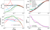 |
Fig. 3 Same as Fig. 2 but for NGC 4636. |
| In the text | |
|
Fig. 4 Best-fit values of 1T (diamond points), 2T (cross), and gdem (empty circles) models to the Chandra ACIS-S simulated data with and without the effect of RS for an exposure time of 500 kiloseconds. The left panels show the best-fit iron abundance values, whereas the right panels show the best-fit values for temperature. The top and bottom panels show the best-fit values for the innermost and the outermost shells, respectively. The shell thickness for most of the objects is approximately between 5 and 6 kiloparsecs for rin and between 80 and 110 kiloparsecs for rout, with the exception of A383 (rin ∈ 5–8.5 kiloparsecs, rout ∈ 66–110 kiloparsecs) and NGC 4636 (rin ∈ 0.3–1.2 kiloparsecs, rout ∈ 12.6–35 kiloparsecs). All best-fit values have been divided by their corresponding input (3D) values. The best-fit values of the 2T model, for which the second CIE component was not significant, were removed from this plot (see last paragraph of Sect. 2.4). The 1T model results of NGC 4636 for the best-fit temperature at rout are plotted with an empty diamond point for visualisation purposes. |
| In the text | |
|
Fig. 5 Emission measure distribution as a function of temperature for the Perseus cluster (left panels) and NGC 4636 (right panels). The different colours represent different shells that were used to extract the input emission measure distribution as described in Sect. 3.1.4 (plotted with histograms). The Gaussian functions in each plot were obtained following Eq. (14) and by using the best-fit values obtained and described in more details in Sect. 3.1. The bottom row shows the radial profile of best-fit values of σ for the Perseus cluster and NGC 4636, where the red and black bars correspond to radial bins used for deriving the EM distribution in the first two rows of this figure. |
| In the text | |
|
Fig. 6 Same as Fig. 4 but for data simulated with the XRISM Resolve micro-calorimeter. The exposure time was assumed to be 200 kiloseconds. The physical sizes of inner shells are approximately (0–3) kiloparsecs for NGC 4636, (0–16) kiloparsecs for Perseus and A262, (0–54) kiloparsecs for A1795, (0–66) kiloparsecs for A2029, and (0–142) kiloparsecs for A383. The physical sizes of outer shells are approximately (3–7) kiloparsecs for NGC 4636, (16–33) kiloparsecs for Perseus and A262, (54–108) kiloparsecs for A1795, (66–133) kiloparsecs for A2029, and (142–283) kiloparsecs for A383. The errors represent the standard deviation 1σ. Similar to Fig. 4, the best-fit values of the 2T model, for which the second CIE component was not significant, were removed from this plot (see the last paragraph of Sect. 2.4). The 1T model results of A383 for the best-fit temperature in both radial bins are plotted with an empty diamond point for visualisation purposes. |
| In the text | |
|
Fig. 7 XRISM Resolve spectra in the energy range 0.6–3 keV simulated with the clus model (including RS) for the 0.3–7 kpc aperture region of NGC 4636 (black points) while assuming the gate valve is open. The best-fit 1T, 2T, and gdem models are plotted with blue, green, and red solid lines together with the residuals that are shown in bottom three panels. The best-fit values of the iron abundance are given in the plots together with 1σ errors. The exposure time was assumed to be 500 ks. |
| In the text | |
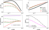 |
Fig. B.1 Same as Fig. 2 but for A2029. |
| In the text | |
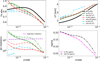 |
Fig. B.2 Same as Fig. 2 but for A1795. |
| In the text | |
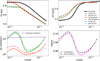 |
Fig. B.3 Same as Fig. 2 but for A262. |
| In the text | |
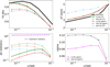 |
Fig. B.4 Same as Fig. 2 but for A383. |
| In the text | |
Current usage metrics show cumulative count of Article Views (full-text article views including HTML views, PDF and ePub downloads, according to the available data) and Abstracts Views on Vision4Press platform.
Data correspond to usage on the plateform after 2015. The current usage metrics is available 48-96 hours after online publication and is updated daily on week days.
Initial download of the metrics may take a while.