| Issue |
A&A
Volume 628, August 2019
|
|
|---|---|---|
| Article Number | A98 | |
| Number of page(s) | 15 | |
| Section | Interstellar and circumstellar matter | |
| DOI | https://doi.org/10.1051/0004-6361/201935731 | |
| Published online | 13 August 2019 | |
A multi-molecular line study of the star-forming globule CB88-230
1
INAF – Istituto di Radioastronomia & Italian ALMA Regional Centre,
Via P. Gobetti 101,
40129 Bologna,
Italy
e-mail: brand@ira.inaf.it
2
East Asian Observatory, 660 N. A’ohoku Place, University Park,
Hilo,
HI 96720,
USA
3
INAF – Osservatorio Astrofisico di Arcetri,
Largo E. Fermi 5,
50125 Florence,
Italy
4
Université Grenoble Alpes, Institut de Planétologie et d’Astrophysique de Grenoble (IPAG),
38401 Grenoble,
France
Received:
18
April
2019
Accepted:
13
June
2019
Context. This paper relates to low-mass star formation in globules, and the interaction of newly-formed stars with their environment. We follow up on the results of our earlier observations of this globule.
Aims. Our aim is to study the gas- and dust environment of the young stellar object (YSO) in globule CB88 230, the large-scale molecular outflow triggered by the jet driven by the YSO, and their interaction.
Methods. We carried out submillimetre continuum and multi-line molecular observations with several single-dish facilities, mapping the core of the globule and the large-scale outflow associated with the YSO.
Results. Dust continuum and molecular line maps (of 12CO, C18O, CS, CH3OH) show a flattened (axes ratio 1.5−1.7), asymmetric core with a full width at half maximum (FWHM)-diameter of 0.16−0.21 pc. Line profiles of 12CO, 13CO(2–1, 3–2), and CS(2–1) show self-absorption near the YSO; the absorption dip is at a slightly (~0.3 km s−1) redder velocity than that of the quiescent gas, possibly indicating infall of cooler envelope gas. The mass of the core, determined from C18O(1–0) observations, is about 8 M⊙, while the virial mass is in the range 5−8M⊙, depending on the assumed density distribution. We detect a slight velocity gradient (~0.98 km s−1 pc−1), though rotational energy is negligible with respect to gravitational and turbulent energy of the core. A fit to the spectral energy distribution of the core gives a dust temperature Td ≈ 18 K and a gas mass of ca. 2 M⊙ (assuming a gas-to-dust ratio of 100). More careful modelling of the sub-mm emission (not dominated by the relatively hot central regions) yields M ≈ 8M⊙. From the molecular line observations we derive gas temperatures of 10−20 K. A Bayesian analysis of the emission of selected molecules observed towards the YSO, yields Tkin ≈ 21.4 K (68% credibility interval 14.5−35.5 K) and volume density n(H2) ≈ 4.6 × 105 cm−3 (8.3 × 10⁴−9.1 × 105 cm−3). We have mapped the well-collimated large-scale outflow in 12CO(3–2). The outflow has a dynamical age of a few 104 yr, and contains little mass (a few 10−2 M⊙). A misalignment between the axis of this large-scale outflow and that of the hot jet close to the YSO indicates that the outflow direction may be changing with time.
Key words: stars: formation / stars: pre-main sequence / ISM: clouds / ISM: jets and outflows / ISM: individual objects: CB88-230
© ESO 2019
1 Introduction
Studies of the molecular environment in star-forming regions are often complicated by the presence of multiple emission line components at different velocities and by young stellar objects (YSOs) in different evolutionary stages stirring up the molecular cloud. This complication can be avoided by selecting a small cloud, such as a Bok globule, which is cold (~10−20 K) and relatively isolated, and in which only one or at most a few low-mass stars are being formed at the same time. Such small clouds consist of a dense core which can be starless, or host an embedded protostar or a slightly more evolved object, surrounded by a lower-density envelope.
A phenomenon associated with the early stages of the formation of stars of all masses are bipolar outflows, which in one scenario are the result of ambient molecular gas being swept up by fast, collimated winds from a YSO. Closest to the YSO one finds the fast, hot, jet-like component that can be detected through H2 ro-vibrational lines at Tex ~ 2000 K and by [FeII]-line emission. Further from the central object the flow cools down and where it hits the gas of the ambient cloud in which the star formation takes place, one may find molecular species with enhanced abundances as a consequence of being produced in a shock-driven chemistry (e.g. SiO, but also SO and CH3 OH; Bachiller 1996 and references therein). The cloud material is entrained by the jet component through turbulent flows or bow-shocks, and is driven away from the YSO to larger distances. This swept-up cloud material is the coolest (Tex ≈ 10−20 K; Bachiller 1996) component and is often easily observable through the emission of the lower-J transitions of CO. Another mechanism by which cloud material can be entrained is by wide-angle winds, launched from the accretion disk around the YSO. This wind blows into the ambient gas and forms a swept-up shell of matter, usually leading to a less collimated flow.
In a previous paper (Massi et al. 2004) we described our search for the jet-component in the near-infrared (NIR) through narrow-band H2 (2.122 μm) and [FeII] (1.644 μm) filters in four star-forming (Bok) globules. In two of the globules H2 and [FeII] emission remained after careful subtraction of the underlying continuum Massi et al. (2004): CB3 and CB230 (LDN1177). The latter is the subject of the present paper1.
CB230 is a 3′.4 × 2′.2 (Clemens & Barvainis 1988) globule at high galactic latitude (13. °16), probably associated with the reflection nebula Sh2-136 (a.k.a. vdB 141). The star illuminating the reflection nebula (BD+67 1300) has a parallax of 2.95 ± 0.35 mas (Gaia Collaboration 2016), meaning a distance of 339(+46, −36) pc2. We also adopted this as the distance to CB230; it is in agreement with the 300 pc used by Tobin et al. (2013), and the 293 ± 54 pc lower limit derived by Das et al. (2015). Embedded in CB230 is a YSO near the position of the IRAS source IRAS 21169+6804 (Lfir ~ 6.5−6.8L⊙; Young et al. 2003; Launhardt & Henning 1997; scaled to d = 339 pc). Yun & Clemens (1994a) detected a bipolar outflow in low-resolution (48′′) 12CO(1–0) observations. Their NIR observations at 1.25 and 2.2 μm (Yun & Clemens 1994b) show a 16′′ conical nebula that is open to the north. The IRAS source is at the apex of this nebula at the NIR peak. It is also detected in (sub)millimetre continuum emission (Launhardt & Henning 1997; Huard et al. 1999; Young et al. 2003; Launhardt et al. 2013). Figure 1 shows an optical image of LDN1177, the reflection nebula and the globule CB230. At the location of the embedded YSO a cone of scattered light is clearly visible.
The jet detected by Massi et al. (2004) in [FeII], originating from the YSO in CB230, is defined by two knots superimposed on a fainter, elongated emission feature (Fig. 5 in Massi et al. 2004). This jet is also traced by H2 emission, which is weaker and slightly less narrow than that of [FeII]. The presence of strong [FeII] and weaker H2 emission suggests the presence of fast, dissociative J-shocks. This is confirmed by the NIR spectra analysed by Massi et al. (2008). These authors also identify the YSO (CB230-A) as a Class 0/I object, confirming the classification by Froebrich (2005). A close companion, ~0′′.3 northeast of CB230-A was found by Tobin et al. (2013); it appeared to be resolved in their high-resolution Very Large Array (VLA) observations at 7.3 mm; its diameter of ~ 45 AU is interpreted by these authors as being indicative of a circumstellar disk. Considering also the embedded binary object (CB230-B1,2) found at about 9′′ east3 of CB230-A by Massi et al. (2004), this globule may contain a quadruple system. In the present paper we present molecular line- and submillimetre continuum data of the outflow and of the core from which it originates and in which the YSO (CB230A) is embedded.
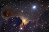 |
Fig. 1 Optical image (LRGB filters) of CB230 and surroundings. Approximate size 19.′5 × 13′. East is left, north is up. The bright patch below the centre with the veiled star BD+67 1300, is the reflection nebula Sh2-136/vdB 141. CB230 is the more opaque structure in the eastern part of the cloud, in which the cone of scattered light, associated with the outflow studied in this paper (Sect. 3.4), is clearly visible. Image credit: Adam Block, Mount Lemon Sky Center, University of Arizona, USA. Used with permission. |
2 Observations and data reduction
The various observations we carried out and which are described in this section, were not all centred on the same coordinates (though within 7′′.4). To facilitate comparison, unless stated otherwise, all offsets in this paper, including the figures, are relative to the YSO position (2MASS-coordinates). In Table 1 we give the positions of the point source detected at the apex of the nebula, as reported by different authors, and the IRAS-position, and the offsets with respect to the 2MASS-position.
Central coordinates used in the observations, and reference coordinates.
2.1 Millimetre lines
Details of the line observations (frequencies, resolution, rms, etc.) can be found in Table 2. All rms-temperatures are in units of  , unless specified otherwise.
2.1.1 James Clerk Maxwell Telescope
On 10 September, 2003 we used RxB3 at the 15-m James Clerk Maxwell Telescope (JCMT) on Mauna Kea (Hawaii) to observe 12CO(3–2) towards CB230 in the raster (on-the-fly) observing mode. The map covers a 90′′ × 230′′ region. The JCMT beamsize at 345 GHz is ~14 ′′; observations were made on an 8′′ raster, using the DAS autocorrelator spectrometer. An off-position was used at offset −600′′ in Declination from the map’s centre position. The low-resolution map of the outflow by Yun & Clemens (1994a) was used to select the area to be observed. We searched for emission of SiO(5–4) (which would trace shock emission) at 5 locations in the outflow.
In the period 26–29 September, and on 4 October 2004 we observed 13CO(3–2) in a 50′′ × 80′′ region towards the central region of the outflow seen in the 12CO(3–2) map. The raster spacing was again 8′′.
In addition, we observed C18O(2–1) at 15 positions along the axis of the outflow. At 4 positions in the outflow we made deeper observations in the J = 2–1 and J = 3–2 transitions of 12CO, 13CO, and C18O, in order to study the line profiles in more detail. Likewise, we searched for SO(65–54) emission (219.9 GHz) at 3 of these positions.
In addition we looked for emission of CS(5–4), HCN(3–2), HCO+(3–2) and (4–3), DCO+(3–2), CH3OH(5k − 4k), and H2 CO(303–202), (322 –221), and (312 –211) at the position of the embedded YSO, which coincides with the centre of the outflow and the peak of the sub-mm continuum observations.
Main beam efficiencies in the 230 and 345 GHz bands were 0.68 and 0.63, respectively.
For line-checks and calibration we observed G34.3, W75N, and NGC7538IRS1. The data were reduced with the program CLASS, which is part of the Gildas-software package developed by the Observatoire de Grenoble and the Institut de Radioastronomie Millimétrique (IRAM).
2.1.2 IRAM 30-m
CB230 was observed simultaneously in 12CO(2–1), 13CO(2–1), CS(2–1), and SO(32–21) with the IRAM 30-m telescope at Pico Veleta (Granada, Spain) in the period August 7–10, 2004. The observations of an area of 60′′ × 104′′ containing the red- and the strongest part of the blue outflow found with the JCMT in 12CO(3–2), were made in the on-the-fly (OTF) observing mode, scanning along mutually orthogonal strips in right ascension and declination. The strips are separated by 4′′. Subsequently, the map was gridded on a 4′′ × 4′′ raster. The reference position for these observations was taken at offset (0′′,−600′′) with respectto the map’s centre position.
In addition SiO(2–1), H13CO+(1–0), CH3OH(2k−1k) and (5–4), and H2 S(220–211) were observed on a 2 × 5-grid, with spacing16′′, centred on (− 9′′, − 2′′) with respectto the YSO-position, using position-switching against the same reference position as above. All spectra were reduced with the Grenoble CLASS software. Low-order polynomial baselines were subtracted.
2.1.3 Onsala
Between May 26 and 31, 2005, we used the 20-m telescope of the Onsala Space Observatory (Sweden) to observe emission of C18O(1–0), CS(2–1) and CH3OH(2k−1k) towards a 4′ × 3′ region in CB230. The observations were carried out in position-switching mode, using a nearby emission-free position as reference. Pointing was regularly checked by observing the SiO(1–0, v = 1) maser emission from TX Cam and R Cas, and was found to be accurate to within 3′′. Observations were carried out using an SIS-mixer and a low-resolution hybrid correlator, which gave a total velocity coverage of about 200 km s−1. Beam efficiencies at 97 and 110 GHz were approximately 0.56 and 0.45, respectively (e.g. Johansson 2002). All spectra were reduced with the Grenoble CLASS software.
2.2 Submillimetre continuum
On September 10, 2003 we simultaneously observed the 450 μm and 850 μm emission towards CB230 with the Submillimetre Common-User Bolometer Array (SCUBA; Holland et al. 1999) at the JCMT. A standard 64-point jiggle map was made, which covers an area 2′.3 in diameter; hence the observations were limited to the region immediately around the IRAS source. The rms values in the CB230 maps were 150 mJy beam−1 (at 450 μm) and 10 mJy beam−1 (at 850 μm), respectively.
Since then, SCUBA-2 observations of superior quality have become available, and we have decided to use these archival data instead.
On June 27–30, 2012 CB230 was observed simultaneously at 450 μm and 850 μm with the Submillimetre Common-User Bolometer Array 2 (SCUBA-2; Holland et al. 2013) at the JCMT. In total six constant velocity (CV) Daisy observations were made on the four nights and retrieved by us from the archive. The 225 GHz optical depth was 0.04−0.05 on all nights, except during the second Daisy on June 28 (due to bad weather) and those data were not used.
CV Daisy observations are designed for small and compact (≲3′) sources, although there is significant exposure time in the map out to 12′. The SCUBA-2 data were reduced with the dynamic iterative map-maker (Chapin et al. 2013) and an isolated source configuration file. Calibration was performed by using water vapour monitor data at 186 GHz, scaled to give the optical depth at 225 GHz, and average ratios of τ(450 μm) and τ(850 μm) to τ(225 GHz). The final transition from instrumental parameters to Jy beam−1 (the flux conversion factor) was derived from calibration observations of Uranus and CRL2688 made on the same night and reduced with the same pixel size as the science observations (see Dempsey et al. 2013). The half-power beamwidths at 450 μm and 850 μm are about 7.9′′ and 13′′, respectively. The rms values in the CB230 maps are 50 mJy beam−1(at 450 μm) and 4 mJy beam−1 (at 850 μm), respectively.
Because the CO(3–2) line is within the bandpass of the SCUBA-2 850 μm filter, these data have been corrected for this contamination which can be significant, in particular at the location of strong outflow sources. We followed the procedure outlined by Parsons et al. (2018), using the CO(3–2) integrated intensity (∫ Tmb dv) map as a negative fake map, to be combined with the SCUBA-2 data in the map maker (see also Drabek et al. 2012). The derived CO-contamination was typically less than 5%.
Details of the molecular line measurements.
2.3 Radio lines
On April 14, 2005 we searched for H2 O(616−523) (22.2350798 GHz) maser emission with the Medicina 32-m telescope4 at the location of the YSO in the core of CB230. In December 2004 we observed CH3OH at four frequencies (23.35–24.96 GHz).
We used a bandwidth of 10 MHz and 1024 channels, resulting in a resolution of 9.76 kHz; the HPBW at 22 GHz was ~1′.7. With our setup only the LHC polarisation is registered. The pointing accuracy was always better than 25′′; the rms residuals from the pointing model were of the order of 8′′ –10′′. Observations were taken in total power mode, with both ON and OFF scans of 5 min duration. The OFF position was taken 1. °25 E of the source position to rescan the same path as the ON scan. Six ON,OFF pairs were taken at this position.
Calibration was done by observing the continuum source DR 21 (for which we assume a flux density of 16.4 Jy after scaling the value of 17.04 Jy given by Ott et al. (1994) for the ratio of the source size to the Medicina beam) at a range of elevations during the day. The typical calibration uncertainty is approximately 20%. For further details on Medicina observations, see Felli et al. (2007).
No detections were made in any of these observations.
3 Results
3.1 Core: dust continuum
In Figs. 2 and 3 we show the SCUBA-2 maps of the dust continuum. Also shown are the intensity profiles along two strips (as indicated in the images).
The continuum emission at 850 μm peaks at offset 0′′,0′′ and thus (see Table 1) coincides with the YSO. At 450 μm the peak lies approximately at offset 0′′,+2′′; in agreement, considering the pixel sizes (2′′ at 450 μm, 4′′ at 850 μm) The emission is asymmetric (more extended to the west) and elongated, with an aspect ratio (extent in RA/extent in Dec) of about 1.5, confirming what is seen in the SCUBA data from Launhardt et al. (2010). The asymmetry is seen also in our own SCUBA observations, but not in the much less sensitive SCUBA images from Huard et al. (1999) and Young et al. 2003. The westward extension of the 850 μm emission traces quite closely the essentially one-sided extinction contours at 8 μm (Tobin et al. 2010). Tobin et al. (2010) argue that these asymmetries are more likely to be due to the initial cloud structure and/or the dynamics of the star formation process, rather than to sculpting by the outflow.
Figure 4 shows the distribution of 350 μm emission observed with the Herschel satellite (Launhardt et al. 2013) in the area observed in different molecular species with the Onsala telescope (see Sect. 3.2.3). The middle-sized white box represents the area in the SCUBA-2 maps in Figs. 2 and 3. The 350 μm emission follows the SCUBA-2 emission except that the western extension in the SCUBA-2 map is a separate peak in the Herschel map.
Flux densities at the two SCUBA-2 wavelengths were calculated by integrating all emission above the 3σ-contour, and sizes of the dust-emission core were determined from the half-peak value contour as well as from the 3σ level, and were corrected for beam size. The results are collected in Table 3.
Figure 5 shows the spectral energy distribution (SED) of CB230. We have plotted our two sub-millimetre data points, in addition to the Herschel flux densities at 70, 100, 160, 250, 350 and 500 μm, extracted from Fig. 4 in Launhardt et al. (2013). We also included a data point at 1.3 mm (Launhardt et al. 2010). We have made a grey-body fit to these data points; the fit is shown as the red curve. The SED-fit shown in Fig. 5 was obtained by assuming a dust opacity ![$k_{\nu} = k_{344.6}(\nu[GHz] / 344.6)^{\beta}$](/articles/aa/full_html/2019/08/aa35731-19/aa35731-19-eq2.png) , with k344.6 = 1.85 cm2 g−1 the opacity at 870 μm (derived from the numbers given in Ossenkopf & Henning 1994) and β =1.8, and a gas-to-dust ratio of 100. This results in Tdust = 18.2 ± 2.0 K and a totalmass derived from the continuum emission Mcont = 1.7 ± 1.0M⊙ at the 95% credibility level. This is virtually identical to the 2.0 M⊙ (when scaled to the same gas-to-dust ratio and distance as used here) derived by Launhardt et al. (2013) from a SED-fit to the integrated fluxes in the core region.
, with k344.6 = 1.85 cm2 g−1 the opacity at 870 μm (derived from the numbers given in Ossenkopf & Henning 1994) and β =1.8, and a gas-to-dust ratio of 100. This results in Tdust = 18.2 ± 2.0 K and a totalmass derived from the continuum emission Mcont = 1.7 ± 1.0M⊙ at the 95% credibility level. This is virtually identical to the 2.0 M⊙ (when scaled to the same gas-to-dust ratio and distance as used here) derived by Launhardt et al. (2013) from a SED-fit to the integrated fluxes in the core region.
To perform a more sophisticated analysis of the dust continuum data, and get a more realistic value of thetotal (gas+dust) mass and investigate the volume density profile of the core, we used RATRAN5 (Hogerheijde & van der Tak 2000). To reproduce the observed flux density distribution of the dust continuum emission we constructed a grid of one-dimensional models of the core. We assumed a gas-to-dust ratio of 100, and a central heating source (Lbol = 6.8L⊙) that gives rise to a temperature profile ∝r−0.4, where r is the distance from the YSO-position, and a density distribution in the core that is ∝ rp, up to a threshold of 2 × 106 cm−3, above which it is assumed to be flat. We varied p between − 1.7 and − 1.5 in steps of − 0.025, and the total mass of the core between 7.2M⊙ and 8.8M⊙, in steps of 0.05M⊙. We focussed on this narrow range in mass after a preliminary, coarser run of models with a larger mass range (0.5−20M⊙). The model was then smoothed with a Gaussian kernel to the angular resolution appropriate for each of the SCUBA2 wavelengths, and compared to the observations with a Bayesian approach. Figure 6 summarises the results of this modelling effort. In panel a we show the observed fluxes at 850 μm in red and at 450 μm in blue, with the best-fit model indicated by the solid lines. The data points represent the flux density for each pixel, and the radial distance is computed from the continuum peak position. The uncertainty of a single point is obtained by summing in quadrature a calibration uncertainty of 20%, the image noise and a fixed term given by the maximum spread between the pixels at similar distances, to mitigate the influence of the elongated structure of the core. Panel b shows the joint probability density of p and mass, as well as their marginalised probability densities in the bottom and right subplots. The best-fit values correspond to p = −1.79 ± 0.15 and M = 8.0 ± 0.5M⊙.
This mass is the same as the one derived from our C18 O-data (see Sect. 3.2.3), but more than four times higher than the 1.7 M⊙ that was derived from the SED-fit. A possible explanation for this discrepancy might be that the fluxes used in the SED-fit are dominated by the relatively hot central region, so that the temperature derived from the SED-fit is overestimated, and the mass underestimated (more representative values for the overall core-temperature are several degrees lower, see Sect. 3.2; for example, for Tdust = 13 K the integrated flux at 850 μm above 3σ implies a total mass M ~ 3.6M⊙). In addition, we made the assumption of symmetry in the model calculation of the dust mass, whereas it is clear from Fig. 2 that the emission is extended more to the west. We have also assumed that the dust core has thesame extent along the line-of-sight as it has in the plane of the sky. These assumptions may lead to an overestimate of the dust- (and thus gas-) mass. In fact, recently Sadavoy et al. (2018) performed a pixel-by-pixel SED-fit to, among others, CB230, using newly zero-point-corrected Herschel data, and find Tdust ≈ 17−19 K at the YSO-location, but 15 ± 1 K around it, and even 13− 14 K just to the west of it (their Fig. 17f). For thecore-region these Tdust-values are very similar to those found in an earlier dust temperature map by Launhardt et al. (2013).
The opacity law that we used in both the RATRAN-modelling and the SED-fit, is that of Ossenkopf & Henning 1994, for grains with thin ice mantles and 105 yr of coagulation. Considering all potential sources of uncertainty, those authors estimate that their tabulated opacities to be accurate to within a factor of two. This implies that also the masses we derive have that overall uncertainty.
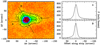 |
Fig. 2 SCUBA-2 map of the dust continuum emission at 850 μm (corrected for CO(3–2) emission; left panel), and profiles along cuts A and B. The 850 μm peak is at (0′′,0′′). Contours (lowest(step)highest) are 12, 20(20)80(80)400(160)720 mJy beam−1. The rms noise is 4 mJy beam−1. |
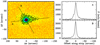 |
Fig. 3 SCUBA-2 map of the dust continuum emission at 450 μm (left panel), and profiles along cuts A and B. The 450 μm peak is at (0′′,2′′). Contours (lowest(step)highest) are 150, 300, 500(500)3500 mJy beam−1. The rms noise is 50 mJy beam−1. |
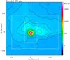 |
Fig. 4 Herschel 350 μm map of the area in CB230 mapped with the Onsala telescope (Sect. 3.2.3). The larger and smaller white box indicate the area of the SCUBA-2 maps (Sect. 3.1) and the IRAM maps (Sect. 3.2.4), respectively. Contour values are 35, 50, 75, 100, 150, 200, 300, 400 MJy sr−1. Offsets are relative to the 2MASS position of the YSO (see Table 1). |
Core parameters derived from the continuum measurements.
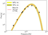 |
Fig. 5 Spectral energy distribution (SED) of CB230. The data shown are the SCUBA-2 measurements at 450 and 850 μm (corrected for CO(3–2)-emission), the integrated flux at 1.3 mm (Launhardt et al. 2010), and the Herschel data points at 70, 100, 160, 250, 350 and 500 μm (extracted from Fig. 4 in Launhardt et al. 2013). The fit to the data (red) was obtained by assuming a dust optical depth at 870 μm of 1.85 cm2g−1, and a dust absorption coefficient β of 1.8. The yellow and green bands indicate the uncertainty in the modelled fluxes for the 68 and 95% credibility intervals of Tdust and Mdust, assuming that the uncertainty on the measured fluxes is 20%. |
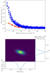 |
Fig. 6 Top panel: flux density (Jy beam−1) as a function of distance (in arcsec) from the YSO-position for 450 (blue) and 850 μm (red). The lines are the best fit model obtained with RATRAN (see text for details). Bottom panel: the joint probability distribution of total (gas + dust) mass and density profile. |
3.2 Core: molecular lines
From our observations of the various isotopologues and transitions of CO, we have several ways to obtain an estimate for the excitation temperature of the gas: from line ratios (3–2)/(2–1) (after the appropriate convolution of the higher-frequency data), or from the peak temperature of the (optically thick) 12CO profiles. In the latter case both IRAM (2–1) and JCMT (2–1) and (3–2) data indicate Tex ≈ 12−14 K for the core and the inner flow (Sect. 3.3), and 10−11 K for locations outside the flow. This is consistent with the derivation through line ratios, where we find Tex ≈ 10−20 K at line centre for locations in the outflow lobes (assuming both lines to be optically thin), with sometimes 25–35 K in the wings. In the case that both lines are assumed optically thick, Tex ~ 7 K at line centre.
3.2.1 Self-absorption
In the central 20′′ × 20′′ of the cloud several of the 12CO(2–1, 3–2) and 13CO(2–1) spectra in the IRAM OTF-maps show a central depression in the emission profile. An example of such a “dip” is shown in Fig. 7a. The maps made at IRAM were centred near the location of the YSO, which is embedded in a cocoon, as revealed by the sub-mm continuum emission (see Sect. 3.1). The YSO itself is only visible in the IR (see Massi et al. 2008), but the conical cavity it has excavated (Massi et al. 2004) is partly optically visible because the cocoon is slightly tilted towards us (cf. Fig. 1; Launhardt 2001). It is thus possible that the central depression in the line profiles is the effect of self-absorption caused by a temperature gradient between the warmer gas near the YSO and the cooler gas further away. In the case of self-absorption the original CO profile might then be reconstructed by fitting a Gaussian profile to the sides of the emission profile, excluding the wings (see Sect. 3.4) and the “dip”. Subtracting the fit from the observed profile and multiplying by − 1 gives the emission removed from the profile by the self-absorption. The distribution of this “missing” emission is shown in Fig. 8. The dip is strongest at offset (+ 3 ′′, + 2 ′′), well within the half-power radius of the submillimetre emission (see Table 3), and therefore supporting the hypothesis of self-absorption.
CB230 is associated with a well-collimated outflow, which we shall discuss in Sect. 3.4. Here, in Fig. 7b, we show the average of all 12CO(2–1) spectra in the blue (Δδ ≥ +2 ′′) and red (Δδ ≤−6 ′′) lobes. Note the very steep red (blue) side on the blue (red) spectrum. In Fig. 7c is shown the average of all spectra at Δα = +27 ′′, well away from the region with the outflow, and therefore representing the quiescent gas. In all spectra three emission components are visible; the ones at − 10 and − 3 km s−1 will be discussed later. The main component of the gas in the globule, at 2.8 km s−1, is very narrow (linewidth ΔV ~ 1.35 km s−1). The dashed lines in Fig. 7 indicate the two peaks in the emission profile in the top panel; they also precisely delimit the quiescent emission. Therefore, the gas at velocities just outside those indicated by the dashed lines already participates in the outflow.
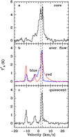 |
Fig. 7 IRAM data. Panel a: a typical 12CO(2-1) profile near the cloud centre. Panel b: average spectrum for Δδ ≤−6 ′′ (red continuous profile) and for Δδ ≥ +2 ′′ (blue histogram). Note the sharp blue- and red edges. Panel c: profile of the quiescent emission: the average of all spectra with Δα = +27 ′′, −54 ′′ ≤ Δδ ≤ 50 ′′. All offsets are relative to the position of the YSO (2MASS coordinates, see Table 1). The dashed lines at 1.9 and 3.4 km s−1 bracket both the “dip” in the CO-profile and the emission of the quiescent gas. |
3.2.2 Multiline analysis
We observed a number of molecules and transitions towards the position of the YSO and the sub-mm peak (see Sect. 3.1). The spectra are shown in Figs. 9 and 10. The relatively large number of molecular lines observed makes it possible to analyse the data with RADEX6, a model for non-local thermodynamic equilibrium (LTE) molecular radiative transfer in an isothermal homogeneous medium. The model requires as input the kinetic temperature, the H2 number density, the molecular column density, and the full width at half maximum (FWHM) of the line; its output is the brightness temperature, the opacity, and the excitation temperature of the lines. The brightness temperature Tb of the lines was estimated from their main-beam brightness temperature Tmb using
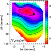 |
Fig. 8 Distribution of the area of the “dip” in the 12CO(2–1) profiles; IRAM data. Contours (lowest(step)highest) are 0.5(0.5)3.5 K km s−1. A Gaussian curve was fitted to each profile (ignoring the “dip” and wings); the fitted profile was subtracted from the original and the result multiplied by −1. The residual was then integrated between 1.3 and 3.4 km s−1. The filled circle indicates the position of the sub-mm peak (see Figs. 2, 3). Offsets are relative to the 2MASS position of the YSO (see Table 1). |
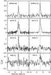 |
Fig. 9 JCMT data. Spectra of various molecular lines at the position of the YSO. The H2 CO(322 − 221) transition was not detected and is not shown (see Table 2). The HCN-spectrum has been Hanning-smoothed to a twice lower resolution with respect to the value in Table 2; the rmsin the spectrum shown is 0.14 K. The dashed line indicates the velocity of the quiescent gas (2.75 km s−1). |
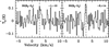 |
Fig. 10 JCMT data. Spectra of SO(65 − 54) at different positions, indicated in the panels. The positions are the peak of the blue (right) and red lobe (left). Offsets are relative to the position of the YSO (2MASS coordinates, see Table 1). The dashed line as in Fig. 9. |
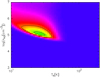 |
Fig. 11 Probability density function for each couple of values |

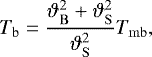 (1)
(1)
where ϑB and ϑS are the FWHM of the beam and the source, respectively. We assumed that all the transitions come from the same region, estimating the source size from the FWHM of the sub-mm and high-resolution CO observations to be about 20′′.
We built a grid of models with different kinetic temperature (Tkin), volume density of molecular hydrogen ( ), and column density of the molecule considered, the first two parameters with 51 equal logarithmic steps (from 10 to 200 K, and from 103 to 107 cm−3, respectively) and the last with 21 (from 5 × 10¹¹ to 1 × 1014 cm−2), respectively. The FWHMof the line is fixed from the observations for each line; only the six lines not affected by self-absorption (CS(5–4), HCN(3–2), SO(65–64), o-H2CO(312–211), p-H2CO(303–202) and (322 –221)) were considered. We used a Bayesian approach (Bolstad 2007) to interpret the results (cf. Giannetti et al. 2012). The probability of measuring a certain value for the intensity of a line is assumed to be represented by a Gaussian curve centred on the value obtained from RADEX for specific physical conditions of the gas, and with a σ given by the uncertainty in the measured value. We used a Gaussian prior on the kinetic temperature, with μ =30 K and σ =30 K. On the other hand, we used a constant prior for the molecular column density and the volume density of molecular hydrogen.
Figure 11 shows the final probability for each combination of Tkin and  . The contours show the 68% and 95% credibility levels. From the marginal probability distributions we find a mean gas temperature log (Tkin[K]) = 1.33 (Tkin = 21.4 K), with a 68% credibility interval for log(Tkin[K]) between 1.16 − 1.55 (14.5 ≤ Tkin ≤ 35.5 K), and a volume density
 ![$\log (n_{\mathrm{H}_2}[\mathrm{cm}^{-3}])=5.66$](/articles/aa/full_html/2019/08/aa35731-19/aa35731-19-eq6.png) , with a 68% credibility interval for
, with a 68% credibility interval for ![$\log (n_{\mathrm{H}_2}[\mathrm{cm}^{-3}])$](/articles/aa/full_html/2019/08/aa35731-19/aa35731-19-eq7.png) between 4.92 − 5.96.
between 4.92 − 5.96.
The lines of HCO+ are self-absorbed, and thus their line temperatures are rather uncertain. We can reconstruct the original line profile by fitting a Gaussian while masking the self-absorbed channels. When we include these lines in the calculations, we take into account a larger uncertainty, given by the difference between the measured line temperature and the one from the reconstructed profile. This then gives log (Tkin(K)) = 1.33 (Tkin = 21.4 K), and 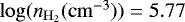 , with a 68% credibility intervals for the logarithmic quantities between 1.05 and 1.52 (10.5 ≤ Tkin ≤ 33.1 K) and 5.00 and 6.20, respectively.
Methanol lines in the observed band at Onsala.
3.2.3 Larger scale
With the various telescopes we mapped the core of CB230 and its immediate surroundings. In Fig. 12 we show the larger-scale emission of C18O(1–0), CS(2–1) and CH3OH(2k−1k) mapped with the Onsala telescope. The three tracers have remarkably different distributions, although they all show an elongated structure; the elongation is roughly perpendicular to the direction of the outflow (see Sect. 3.4). The contours at half the peak value indicate a flattening of a factor of 1.5−1.7 (extent in RA/extent in Dec); the area under this contour gives an equivalent beam-corrected core diameter of 0.16 pc (CH3OH) or 0.21 pc (C18O, CS).
With Tex ≈ 15 K and assuming C18O is optically thin, we derive from the detection equation that τ[C18O(1–0)] ≈ 0.18 for the average C18O spectrum inside the half-maximum contour and an average column density of N(C18O) = 1.5 × 1015 cm−2. Using [C18O]/[H2] = 1.7 × 10⁻⁷ (Frerking et al. 1982), the average N(H2) = 9.0 × 1021 cm−2. The total molecular mass inside the FWHM contour is therefore about 7.6 M⊙, including a correction (× 1.36) for helium and metals. With an average C18O linewidth of 0.60 km s−1 inside the FWHM-contour (which has an equivalent radius of 0.11 pc), we derive a virial mass of 5.0 or 8.3M⊙ for a density distribution ∝r−2 or constant, respectively.
Likewise we find N(CS) ≈ 3.6 × 1012 cm−2 (assuming CS(2–1) is optically thin) and a mass inside the FWHM contour of 3.30 × 10⁻⁹ ([CS]/[H2])−1. With an abundance [CS]/[H2] = 2.0 × 10⁻⁹ (Zhou et al. 1991) we get M ≈ 1.7M⊙, which is likely a lower limit because the CS profiles in the core-region suffer from self-absorption. Correcting for optical depth would increase this lower limit by a factor of 1.6−2.3 for τ = 1−2, respectively.
Table 4 lists the methanol lines that fall within the bandwidth of the Onsala spectra. Where a detection was made, the two lower frequency lines were virtually always detected together (except at offset (42′′,−40′′), where only the A+ component was detected). The third line in the table was detected only at offset (4′′,74′′). In Fig. 12b the contours for methanol indicate the sum of the emission all detected lines, while in Figs. 12c and d we show the integrated emission for the A+ and E-components separately. The latter has an upper energy level almost twice as high as the former, and its emission is more concentrated around the YSO; the A+ component on the other hand, has a more elongated distribution. Methanol is commonly detected in dark clouds; it is expected to be enhanced in regions with shocks, but there is no sign of this along the large-scale CO outflow (cf. Fig. 12b). In fact we see that the CH3OH(2–1) emission peaks at the YSO-position and is more extended perpendicular to the outflow direction.
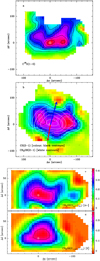 |
Fig. 12 Onsala data. Panel a: C18O(1–0) ∫Tmbdv. Lowest contour and step: 0.6 and 0.2 K km s−1; panel b: CS(2–1) ∫Tmbdv (colour scale and black contours; lowest contour and step: 0.35, 0.2 K km s−1) with CH3OH(2–1) ∫Tmbdv (white contours; lowest contour and step: 0.15 K km s−1) superimposed; the combined area under the two emission lines with the lowest upper level temperature (E and A+; Table 4 and Fig. 14) are shown. The red and blue arrows indicate the approximate direction of the outflow detected in CO(3–2) (see text). The small white crosses indicate the positions where both CS and CH3 OH were observed; the black dots are for CS only. Panel c: CH3OH(2–1) ∫Tmbdv for the A+ component (see Fig 14) only. Lowest contour and step: 0.15, 0.1 K km s−1. Panel d: as c, but for the E-component only. In all panels, the white crossed circle indicates the position of the 850 μm peak, which is also that of the embedded YSO. All offsets are relative to the 2MASS YSO position (see Table 1). |
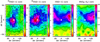 |
Fig. 13 IRAM data. 12CO, 13CO, CS, and SO |

3.2.4 Smaller scale
The smaller-scale maps made with the IRAM 30-m telescope (Fig. 13) confirm the differences in gas distribution seen on the larger-scale. While the 12CO(2–1) and 13CO(2–1) emission have a maximum also at the location of the YSO, the CS(2–1) does not; CS, a tracer of volume density, has a reduced presence in the cavity cleared out by the outflow at the location of the YSO. At the same time, the CS(2–1) profiles show signs of self-absorption in the vicinity of the YSO, which also reduces the integrated intensity. (cf. Fig. 2 in Tobin et al. 2010, where the extinction, represented by the optical depth at 8 μm, is higher and more extended to the West of the YSO). Interestingly, in both 12CO and 13CO we find the peak at about 10′′ east of the YSO, which coincides with the location of the NIR source found by Yun & Clemens (1994b) and resolved as binary source CB230-B1 and -B2 by Massi et al. (2004).
With the IRAM 30-m telescope we made higher-resolution and deeper observations of both CH3OH(2–1) and (5–4) at ten positions, along two parallel strips (see Sect. 2.1.2). The two lowest-excitation lines were detected everywhere, while a third component was clearly detected at the position of the YSO and only marginally at a few other locations. The (5–4) transition was detected nowhere. With only 2 or even 3 detected lines it is difficult to determine the physical parameters of the gas. Nevertheless we fitted synthetic spectra to the observations, using MCWeeds (Giannetti et al. 2017). This program allows one to simultaneously fit lines from an arbitrary number of species and components, in multiple spectral ranges, assuming LTE conditions. We ran MCWeeds on the single spectrum at the YSO position as well as on the average spectrum of those positions where the third emission component of the (2–1) transition was (marginally) detected (see Fig. 14). The (5–4) spectrum was also used by the routine; even though no lines were detected, this serves to constrain the kinetic temperature. The results are quite similar, and we only show those for the average spectrum, in Fig. 14. The fit results are Tex ≈ 7.6 ± 0.6 K, log (N) ≈ 13.40 ± 0.07, but it is clear from the lower panel of the figure, that the fit is not good: it overestimates the intensity of the higher-frequency E-line and severely underestimates that of the lower-frequency E-component. This implies that either methanol is not in LTE and/or that the various components come from regions of different temperature and density.
Several other molecules have been observed on the same 2 × 5 grid (see Table 2 and Sect. 2.1.2): SiO(2–1) and H2 S(220−211) have not been detected anywhere, while H13CO+(1−0) has been detected at all positions except the bottom row (Δδ = −34 ′′). This line was detected in the low-resolution broadband backend of the SiO(2–1) observations. Because of the poor velocity resolution (3.45 km s−1) the emissionis in only one channel. The rms-values of the non-detections translate into an upper limit to the column densities of 1.0 × 1012 cm−2 for SiO, and 1.8 × 1013 cm−2 for H2S. These are 3σ limits calculated using Weeds, from ∫ Tmb dv when integrating over 2 km s−1, and assuming Tex = 100 K. A high value for the temperature is used here, because these molecules are produced by sputtering or shattering of dust refractory cores.
With the JCMT we observed SiO(5–4) at 5 positions in the molecular outflow (see Sect. 3.4; 3 in the blue lobe, 2 in the red lobe); no emission was detected. These non-detections imply a 3σ upper limit to the column density of about 7.1 × 1011 cm−2 (from Weeds; and Tex = 100 K).
Massi et al. (2008), from [FeII]-spectral lines, estimated the hydrogen volume density in the knots in the jet to be nH ~ 104−3 × 105 cm−3. Considering that the size of, for example, knot k1 is ~ 1′′.2 (Massi et al. 2004), this implies a column density of N(H) ~6 × 10¹⁹−1.8 × 1021 cm−2 (for d = 339 pc). In shocks the abundance of SiO can be very much enhanced relative to its abundance in the quiescent medium; for example in dark cloud L1448 it reaches values of a few × 10−7 in the outflow driven by the embedded low-mass protostar (Bachiller et al. 1991). The above-mentioned range of N(H) would then imply N(SiO) ~ 1012−1014 cm−2, higher than the upper limits estimated above. It is possible that SiO is present in the jet, but is undetected with the JCMT because of beam dilution.
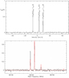 |
Fig. 14 IRAM 30-m data. Top panel: average CH3OH(2 − 1) spectrum of observations at 6 positions in which the three indicated lines are detected. The spectrum has been smoothed to a resolution of 0.484 km s−1; rms = 0.014 K. Bottom panel: fit (in red) to the same average spectrum (at original resolution of 0.242 km s−1, and shown in frequency scale). See text for details. |
3.3 Velocity gradient
Figure 15 shows that the C18O emission has a velocity gradient across the core. The figure shows the line velocities as a function of Δα at Δδ = 0′′, which is roughly perpendicular to the north-south orientation of the outflow (see Sect. 3.4). In these Onsala data this tracer shows a small gradient, with velocities being bluer on the western side of the core. The gradient is 0.98 km s−1 pc−1; if this were to be taken as rotation, this would correspond to an angular velocity ω ≈ 3.2 × 10⁻¹⁴ s−1. This puts CB230 somewhere near the region of “fast” rotators, according to the distribution found by Kane & Clemens (1997) for starless Bok globules. We note that we are not able to determine a trustworthy velocity gradient using the IRAM CS-data, because many line profiles in the central region suffer from self-absorption, making it difficult to determine an accurate velocity of the actual, unaffected profile.
Velocity gradients in the core have been detected before, in N2 H+(1–0) (Chen et al. 2007; Tobin et al. 2011) and NH3(1,1) (Tobin et al. 2011). On the large-scale, comparable to that in Fig. 15, the single-dish N2 H+ observations by Tobin et al. (2011), scaled to a distance of 339 pc, show a gradient of about 2.3 km s−1 pc−1, with velocities decreasing from east to west (cf. Fig. 15). However, when measured over the inner 20′′ − 40′′, the gradients are − 2.8 km s−1 pc−1 for the single-dish N2 H+ observations(Tobin et al. 2011) and of the order of − 10.4 to − 9.7 km s−1, pc−1 from the interferometric observations of N2 H+ (Chen et al. 2007) and NH3 (Tobin et al. 2011), all when scaled to a distance of 339 pc. The minus sign indicates a change in direction of the velocity gradient; in the inner ±10−20 ′′ around the YSO, the velocities increase from east to west. This reversal of velocity gradient on the small scale indicates that the disk around the protostellar binary is apparently physically decoupled from the rest of the cloud.
With the measured gradient of Vgrad = 0.98 km s−1 pc−1, the ratio of the rotational kinetic energy and gravitational energy is  , for a homogeneous spherical core; for a core with a density ∝r−2 this would be three times smaller (Goodman et al. 1993). Likewise the rotational kinetic energy is only a small fraction (≈ 1%) of the turbulent energy (Eturb = (1∕2)MΔV2; ΔV ~ 0.6 km s−1 for C18O). It is thus clear that rotation is not relevant for the energy budget of the cloud (-core).
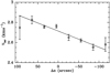 |
Fig. 15 Onsala data. C18O(1–0) velocity (from Gaussian fit to line profiles) at Δδ = 0′′ vs. Δα (see Fig. 12a). Drawn line is best fit, and indicates velocity gradient of 0.98 km s−1 pc−1. Offsets are relative to the position of the YSO (2MASS coordinates, see Table 1). |
3.4 Large-scale outflow
The average 12CO(2–1) spectrum of the quiescent cloud emission in Fig. 7c shows that in addition to the main emission component at ~ 2.7 km s−1 there is also emission at approximately −10 and − 3 km s−1. The outflowing gas is characterised by broad wings on the line profiles that can extend out to − 7 and +14 km s−1, and thus at certain locations in the map includes the − 3 km s−1 component. The − 10 km s−1 component is well outside the range of the blue wing emission, and is clearly not connected to CB230 as it peaks outside (to the SE) the region mapped here. Inside the mapped region it has an irregular distribution (see Fig. 16). Emission at − 3 km s−1 is not very strong and does not significantly contribute to the total emission in the blue wings, but including this velocity component in the integral over the line wings outside the region of the outflow leads to regions of enhanced blue-wing emission which is not real as it is not part of the blue wing at all. We have therefore Gaussian-fitted and removed this component from all spectra where it was clearly separate from the blue wing.
The map of the outflow emission is shown in Fig. 17. Integration limits in velocity were chosen such that they exclude the emission of the quiescent gas. To determine the velocity at which the gas may be considered to partake in the outflow, we have fitted a Gaussian curve to the line profile at the centre using a mask that excludes both the self-absorption dip and the extended wings, see Fig. 18. This should more or less reproduce the original emission profile. The velocities at which the quiescent emission ends were then taken to be those at which the Gaussian profile reaches the half-intensity value.
The blue lobe is much more extended than the red one; this may indicate that the outflow is somewhat tilted towards us causing us to have a protracted view of the gas at red-shifted velocities. On the other hand, a glance at Fig. 1 suggests that this could also be because south of the YSO the edge of the globule is reached sooner than in the north, so there simply is no more material to participate in the outflow. An overlay of the molecular outflow and the hot jet was shown in Fig. 1 in Massi et al. (2008): there is a directional offset between the position angle of the jet seen in [FeII] emission, and that of the large-scale molecular outflow, of about 15°. The light cone seen in Fig. 1 lies more or less in the same direction as the [FeII]-jet, while the molecular outflow hugs the western edge of the light cone. This misalignment suggests that perhaps the outflow has changed direction with time: the current molecular flow is the material swept up when the jet was pointing in that direction; when the jet precesses it takes time before enough new cloud material is being entrained and becomes detectable. This causes an offset between the jet and the central axis of the molecular outflow.
We calculated the parameters of the outflowing gas, by assuming LTE-conditions and optically thin gas. The results are shown in Table 5. We considered two values of Tex (see Sect. 3.2) and used Tmb. The total velocity intervals over which we integrated are − 5.63 to 1.37 km s−1 (blue wing) and 4.68–13.68 km s−1 (red wing). Integration was done in 1 km s−1-wide bins; emission with S/N = 3 and 2 was taken into account, respectively (top and bottom parts in Table 5). In addition to the mass of the material participating in the outflow, we also calculated the flow’s momentum, energy, size and velocity (cf. Wouterloot & Brand 1999; Lada 1985). The dynamical age (tdyn) was then derived from the ratio of the size of the flow and its velocity. The age was used to derive the force Fm (=Momentum/age) required to drive the outflow and the mechanical luminosity Lm (=Energy/age). It is no surprise that this low-mass dark cloud and its low-mass YSO (0.2−0.5M⊙, Froebrich 2005; ~ 0.3M⊙, Massi et al. 2008; all scaled to 339 pc) are associated with a low-mass outflow, with Mtot ≈ (1−3) × 10−2 M⊙ (~ 0.1−0.4% of the core mass), depending on the value of Tex.
In these calculations we have not taken into account the inclination of the outflow with respect to the plane of the sky. For an inclination angle i the correction in outflow velocity is 1/sin (i), while the size of the flow should be corrected by 1/cos (i). The derived age would change by a factor of tan (i). So for i = 30° the flow would be 42% younger, and for i = 60° (less likely) it would be 73% older. Momentum and energy would need to be adjusted by a factor of 1/sin (i) and (1/sin (i))2, respectively. The masses need no correction.
By comparing the momentum flux of the atomic jet, seen in [FeII]-emission, and that of the larger-scale molecular outflow, Massi et al. (2008) have concluded that the jet is capable of driving the molecular outflow. If the outflow has a semi-aperture angle θ, then the fraction of the (spherical) core mass that is swept away by the jet is  (1−cosθ) for each of the lobes. The total mass in the outflow is (Tex = 15 K; emission > 3σ) Mtot ~ 1.4 × 10⁻² M⊙, which is 0.18% of the core mass (8 M⊙; Sect. 3.1, Fig. 6). This implies θ ≈3. °4 and an opening angle of 6. °8. For the (more massive) blue lobe alone the opening angle is found to be 8. °2. That is approximately the same as the angle subtended by knot k1 in the jet (see Massi et al. 2004), as seen from the YSO. The total angle covered by the cone of [FeII]-emission is about 63°; if, as mentioned earlier, the outflow has changed direction with time, this may be the angle that the jet has swept out, not necessarily the opening angle of the outflow. Some of the mass in the large-scale outflow does not come from the core but is swept-up cloud material. Considering the blue lobe, and assuming that 30− 50% of the mass in the outflow is swept-up ambient cloud material, we find an opening angle of 6°–7°, still very similar to the jet-angle.
Figures 19 and 20 (deep integrations towards 4 selected positions in the outflow; JCMT data) show the narrowness of the quiescent gas emission [ΔVFWHM ~ 1 km s−1 for C18O(2–1, 3–2)]. In these higher-resolution spectra (compared to the ones in Fig. 7) we also see that the velocity of the self-absorption dip is actually slightly redder than the velocity of the quiescent gas. This could be a sign of infalling cooler gas from the envelope. The spectra in Fig. 20 show that the outflow is only clearly visible in 12CO, although Fig. 17 shows that also 13CO profiles havedetectable red- and blue-shifted emission.
In Fig. 17 we have indicated several locations along the outflow lobes where we have obtained C18O(2–1) spectra. These are shown in Fig. 21. We have made Gaussfits to these spectra; the average velocities in the red lobe (2.882 ± 0.042 km s−1) are redder than those in the blue lobe (2.744 ± 0.069 km s−1), but no velocity gradient along the outflow lobes is detected.
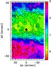 |
Fig. 16 IRAM data. Distribution of |
![$T^*_{\textrm{A}}[{}^{12}\textrm{CO}(2-1)]$](/articles/aa/full_html/2019/08/aa35731-19/aa35731-19-eq13.png)
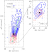 |
Fig. 17 JCMT data. Left panel: distribution of |

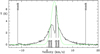 |
Fig. 18 Gaussfit to the emission profile of 12CO(3–2) at the centre position of the outflow (−8′′,0′′). A mask wasused as indicated to exclude the self-absorption dip and the extended line wings. |
Parameters of the molecular outflow associated with CB230.
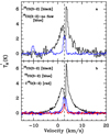 |
Fig. 19 JCMT data. Comparison of spectra at the location of the YSO (coinciding with the centre of the outflow and the sub-mm continuum peak). Panel a: 12CO(3–2) spectrum (broad emission line; taken from the mapping data). The weaker, narrow blue line is the average of 45 spectra in the 12CO(3–2)-map, with α > 25′′, well away from the outflow and hence representing the quiescent gas. The dashed line indicates its central velocity (2.75 km s−1), which corresponds with that of the dip in the line profile at the centre of the outflow, while the width of the dip is virtually identical to the fwhm of the quiescent gas profile. Panel b: deep J=3–2 spectra of three CO-isotopologues. Only C18O (red) does not show a self-absorption dip. The velocity of its peak nearly coincides with the central velocity of the quiescent gas in panel a. |
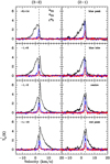 |
Fig. 20 JCMT data. Comparison of J = 3–2 (left) and J = 2–1 (right) spectra at four positions of 12CO (black), 13CO (blue), and C18O (red). The widest and most intense emission is that of 12CO, the narrowest and weakest emission profile is that of C18O. The dashed line indicates the velocity (2.75 km s−1) of the quiescent gas (see Fig 19). The offsets relative to the 2MASS YSO position are indicated in the left-hand panels (see also Fig. 17). |
4 Summary
We have carried out a multi-molecular line and sub-mm continuum study of globule CB88 230 (CB230 for short) with various single-dish antennas. The aim was to study the molecular outflow associated with the jet we discovered emanating from the YSO (Massi et al. 2004), as well as the cloud surrounding the YSO, a low-mass (~ 0.3M⊙; scaled to a distance of 339 pc) Class 0/I object (Massi et al. 2008). CB230 is found to have a flattened core, material distributed asymmetrically with respect to the embedded YSO and showing self-absorbed line profiles, that may indicate infalling colder gas from the envelope. The YSO is associated with a low-mass bipolar outflow with the northern (blue) lobe tilted towards the observer, allowing a partially unobscured look into the cone excavated by the flow. Our main results can be summarised as follows:
Larger-scale line maps (C18O, CS, CH3OH) show a flattened core structure (ratio 1.5–1.7), with equivalent beam-corrected diameter 0.16−0.21 pc. Also the submillimetre dust continuum observations show a flattened structure, an equivalent diameter (at 850 μm) of ~ 0.16 pc, and an asymmetry with respect to the YSO. This asymmetry is also visible in the line maps of CS, SO and C18O.
The line ratios of optically thin lines indicate an excitation temperature of 10− 20 K as does the line intensity of the optically thick 12CO-lines. A fit to the SED results in a dust temperature of ~18 K.
A multi-line analysis of molecules observed towards the YSO, using Bayesian approach finds a mean gas temperature of 21.4 K (with a rather large 68% credibility interval of 14.5–35.5 K), and an H2 volume density n ≈ 4.6 × 105 cm−3 (8.3 × 10⁴−9.1 × 10⁵).
Assuming LTE-conditions, we find a molecular mass inside the FWHM contour of M ≈ 8M⊙, from our C18O(1–0) observations. The virial mass is ~ 5−8M⊙, depending on the assumed density distribution. From modelling the dust-continuum observations we find a total gas mass of 8 M⊙, assuming a gas-to-dust ratio of 100. The SED fit yields about 2 M⊙, which is likely too low because the SED is dominated by the emission from the relatively hot central region (and higher temperature leads to lower mass-estimates).
Line profiles of 12CO, 13CO, HCO+ and CS(2–1) in the immediate vicinity of the YSO show self-absorption. Observations at higher velocity-resolution show that the self-absorption dip is at a slightly redder velocity than that of the quiescent gas emission, suggesting infall of cooler gas.
A well-collimated molecular outflow is associated with the YSO. We mapped the outflow in 12CO(3–2). Away from the flow-region, the profiles of the quiescent gas are quite narrow (~ 1 km s−1). The blue lobe is longer than the red lobe, most likely because the edge of the globule is nearer to the YSO towards the south than towards the north and there just is no more material to participate in the flow.
The flow has a dynamic age of a few 104 yr, and contains very little mass (a few 10−2 M⊙). The calculated age depends on the inclination angle i of the flow relative to the plane of the sky as tan (i). A misalignment of ~ 15° between theaxis of the molecular outflow and the direction of the hot jet detected previously (see Massi et al. 2004) suggests a change in outflow direction (precession) with time. The mass of the gas participating in the outflow is consistent with the fraction of the core-mass being swept away by the jet as seen in [FeII], with an opening angle of ~ 8°, even when taking into account that a large fraction of the outflow mass is entrained ambient cloud material.
Molecules, such as H2S and SiO, that are expected to show an enhanced abundance in regions where shocks occur (e.g. where the fast jet hits the ambient medium), have not been detected. The non-detections imply upper limits to the column densities of 1.0 × 1012 cm−2 for SiO and 1.8 × 1013 cm−2 for H2S. The non-detection of SiO(5–4) at several locations in the outflow implies an upper limit of the column density of ~ 7.1 × 1011 cm−2. Only SO(65−54) has been (marginally) detected at two locations in the outflow, though still near the YSO.
A modest velocity gradient (0.98 km s−1 pc−1) is detected in C18O, roughly perpendicular to the outflow axis. If this is core-rotation, a comparison with gravitational and turbulent energy shows that rotation is not relevant for the energy budget of the core (only ~ 1% of the total energy).
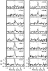 |
Fig. 21 JCMT data. C18O(2–1) spectra taken along the CO-outflow axis (see Fig. 17). Dashed line as in Fig. 19. Offsets are in arcsec relative to the 2MASS YSO position (see Table 1). |
Acknowledgements
The James Clerk Maxwell Telescope has historically been operated by the Joint Astronomy Centre on behalf of the Science and Technology Facilities Council of the UK, the National Research Council of Canada and The Netherlands Organization for Scientific Research. The line data were taken for project M03BI06 and M04BI07; the SCUBA observations were part of project M03BI06. This work makes use of archival SCUBA-2 data (project M12AC18). Additional funds for the construction of SCUBA-2 were provided by the Canada Foundation for Innovation. This work has benefitted from research funding from the European Community’s Sixth Framework Programme. This research has made use of NASA’s Astrophysics Data System Bibliographic Services (ADS) and of the SIMBAD database, operated at CDS, Strasbourg, France. This work has made use of data from the European Space Agency (ESA) mission Gaia (https://www.cosmos.esa.int/gaia), processed by the Gaia Data Processing and Analysis Consortium (DPAC, https://www.cosmos.esa.int/web/gaia/dpac/consortium). Funding for the DPAC has been provided by national institutions, in particular the institutions participating in the Gaia Multilateral Agreement. C.C. acknowledges the project PRIN-INAF 2016 The Cradle of Life - GENESIS-SKA (General Conditions in Early Planetary Systems for the rise of life with SKA). We are grateful to Dr. Adam Block (Mount Lemon Sky Center, Univ. of Arizona) for permission to use the optical image of CB230 and its surroundings (Fig. 1).
References
- Bachiller, R. 1996, ARA&A, 34, 111 [NASA ADS] [CrossRef] [Google Scholar]
- Bachiller, R., Martin-Pintado, J., & Fuente, A. 1991, A&A, 243, L21 [NASA ADS] [Google Scholar]
- Bolstad, W. M. 2007, Introduction to Bayesian Statistics (Hoboken, NJ: Wiley) [CrossRef] [Google Scholar]
- Chapin, E. L., Berry, D. S., Gibb, A. G., et al. 2013, MNRAS, 430, 2545 [NASA ADS] [CrossRef] [Google Scholar]
- Chen, X., Launhardt, R., & Henning, T. 2007, ApJ, 669, 1058 [NASA ADS] [CrossRef] [Google Scholar]
- Clemens, D. P., & Barvainis, R. 1988, ApJS, 68, 257 [NASA ADS] [CrossRef] [Google Scholar]
- Das, A., Das, H. S., & Senorita Devi, A. 2015, MNRAS, 452, 389 [NASA ADS] [CrossRef] [Google Scholar]
- Dempsey, J. T., Friberg, P., Jenness, T., et al. 2013, MNRAS, 430, 2434 [Google Scholar]
- Drabek, E., Hatchell, J., Friberg, P., et al. 2012, MNRAS, 426, 23 [NASA ADS] [CrossRef] [Google Scholar]
- Felli, M., Brand, J., Cesaroni, R., et al. 2007, A&A, 476, 373 [NASA ADS] [CrossRef] [EDP Sciences] [Google Scholar]
- Frerking, M. A., Langer, W. D., & Wilson, R. W. 1982, ApJ, 262, 590 [NASA ADS] [CrossRef] [Google Scholar]
- Froebrich, D. 2005, ApJS, 156, 169 [NASA ADS] [CrossRef] [Google Scholar]
- Gaia Collaboration (Brown, A. G. A., et al.) 2016, A&A, 595, A2 [NASA ADS] [CrossRef] [EDP Sciences] [Google Scholar]
- Gaia Collaboration (Brown, A. G. A., et al.) 2018, A&A, 616, A1 [NASA ADS] [CrossRef] [EDP Sciences] [Google Scholar]
- Giannetti, A., Brand, J., Massi, F., Tieftrunk, A., & Beltrán, M. T. 2012, A&A, 538, A41 [NASA ADS] [CrossRef] [EDP Sciences] [Google Scholar]
- Giannetti, A., Leurini, S., Wyrowski, F., et al. 2017, A&A, 603, A33 [NASA ADS] [CrossRef] [EDP Sciences] [Google Scholar]
- Goodman, A. A., Benson, P. J., Fuller, G. A., & Myers, P. C. 1993, ApJ, 406, 528 [NASA ADS] [CrossRef] [Google Scholar]
- Hogerheijde, M. R., & van der Tak, F. F. S. 2000, A&A, 362, 697 [NASA ADS] [Google Scholar]
- Holland, W. S., Robson, E. I., Gear, W. K., et al. 1999, MNRAS, 303, 659 [NASA ADS] [CrossRef] [MathSciNet] [Google Scholar]
- Holland, W. S., Bintley, D., Chapin, E. L., et al. 2013, MNRAS, 430, 2513 [NASA ADS] [CrossRef] [Google Scholar]
- Huard, T. L., Sandell, G., & Weintraub, D. A. 1999, ApJ, 526, 833 [NASA ADS] [CrossRef] [Google Scholar]
- Johansson, L. E. B. 2002, The 20-m Telescope Handbook (Sweden: Onsala Space Observatory) [Google Scholar]
- Kane, B. D., & Clemens, D. P. 1997, AJ, 113, 1799 [NASA ADS] [CrossRef] [Google Scholar]
- Lada, C. J. 1985, ARA&A, 23, 267 [NASA ADS] [CrossRef] [Google Scholar]
- Launhardt, R. 2001, The Formation of Binary Stars, IAU Symp., eds. H. Zinnecker & R. D. Mathieu (San Francisco: ASP), 200 [Google Scholar]
- Launhardt, R., & Henning, Th. 1997, A&A, 326, 329 [NASA ADS] [Google Scholar]
- Launhardt, R., Nutter, D., Ward-Thompson, D., et al. 2010, ApJS, 188, 139 [NASA ADS] [CrossRef] [Google Scholar]
- Launhardt, R., Stutz, A. M., Schmiedeke, A., et al. 2013, A&A, 551, A98 [NASA ADS] [CrossRef] [EDP Sciences] [Google Scholar]
- Massi, F., Codella, C., & Brand, J. 2004, A&A, 419, 241 [NASA ADS] [CrossRef] [EDP Sciences] [Google Scholar]
- Massi, F., Codella, C., Brand, J., DiFabrizio, L., & Wouterloot, J. G. A. 2008, A&A, 490, 1079 [NASA ADS] [CrossRef] [EDP Sciences] [Google Scholar]
- Ossenkopf, V., & Henning, T. 1994, A&A, 291, 943 [NASA ADS] [Google Scholar]
- Ott, M., Witzel, A., Quirrenbach, A., et al. 1994, A&A, 284, 331 [NASA ADS] [Google Scholar]
- Parsons, J., Dempsey, J. T., Thomas, H. S., et al. 2018, ApJS, 234, 22 [NASA ADS] [CrossRef] [Google Scholar]
- Sadavoy, S. I., Keti, I., Bourke, T. L., et al. 2018, ApJ, 852, 102 [NASA ADS] [CrossRef] [Google Scholar]
- Tobin, J. J., Hartmann, L., Looney, L. W., & Chiang, H.-F. 2010, ApJ, 712, 1010 [NASA ADS] [CrossRef] [Google Scholar]
- Tobin, J. J., Hartmann, L., Chiang, H.-F., et al. 2011, ApJ, 740, 45 [NASA ADS] [CrossRef] [Google Scholar]
- Tobin, J. J., Chandler, C. J., Wilner, D. J., et al. 2013, ApJ, 779, 93 [NASA ADS] [CrossRef] [Google Scholar]
- van der Tak, F. F. S., Black, J. H., Schöler, F. L., Jansen, D. J., & van Dishoeck, E. F. 2007, A&A, 468, 627 [NASA ADS] [CrossRef] [EDP Sciences] [Google Scholar]
- Wouterloot, J. G. A., & Brand, J. 1999, A&AS, 140, 177 [NASA ADS] [CrossRef] [EDP Sciences] [Google Scholar]
- Young, C. H., Shirley, Y. L., Evans, N. J. II, & Rawlings, J. M. C. 2003, ApJS, 145, 111 [NASA ADS] [CrossRef] [Google Scholar]
- Yun, J. L., & Clemens, D. P. 1994a, ApJS, 92, 145 [NASA ADS] [CrossRef] [Google Scholar]
- Yun, J. L., & Clemens, D. P. 1994b, AJ, 108, 612 [NASA ADS] [CrossRef] [Google Scholar]
- Zhou, S., Evans, N. J. II, Güsten, R., et al. 1991, ApJ, 372, 518 [NASA ADS] [CrossRef] [Google Scholar]
Gaia Collaboration (2018) lists the parallax of this star as 2.9075 ± 0.0208 mas, that is a distance of 343.94(+2.48, −2.44) pc, a difference of only ~1.5% with the value adopted here.
In Massi et al. (2004) it erroneously says “west”.
All Tables
All Figures
|
Fig. 1 Optical image (LRGB filters) of CB230 and surroundings. Approximate size 19.′5 × 13′. East is left, north is up. The bright patch below the centre with the veiled star BD+67 1300, is the reflection nebula Sh2-136/vdB 141. CB230 is the more opaque structure in the eastern part of the cloud, in which the cone of scattered light, associated with the outflow studied in this paper (Sect. 3.4), is clearly visible. Image credit: Adam Block, Mount Lemon Sky Center, University of Arizona, USA. Used with permission. |
| In the text | |
|
Fig. 2 SCUBA-2 map of the dust continuum emission at 850 μm (corrected for CO(3–2) emission; left panel), and profiles along cuts A and B. The 850 μm peak is at (0′′,0′′). Contours (lowest(step)highest) are 12, 20(20)80(80)400(160)720 mJy beam−1. The rms noise is 4 mJy beam−1. |
| In the text | |
|
Fig. 3 SCUBA-2 map of the dust continuum emission at 450 μm (left panel), and profiles along cuts A and B. The 450 μm peak is at (0′′,2′′). Contours (lowest(step)highest) are 150, 300, 500(500)3500 mJy beam−1. The rms noise is 50 mJy beam−1. |
| In the text | |
|
Fig. 4 Herschel 350 μm map of the area in CB230 mapped with the Onsala telescope (Sect. 3.2.3). The larger and smaller white box indicate the area of the SCUBA-2 maps (Sect. 3.1) and the IRAM maps (Sect. 3.2.4), respectively. Contour values are 35, 50, 75, 100, 150, 200, 300, 400 MJy sr−1. Offsets are relative to the 2MASS position of the YSO (see Table 1). |
| In the text | |
|
Fig. 5 Spectral energy distribution (SED) of CB230. The data shown are the SCUBA-2 measurements at 450 and 850 μm (corrected for CO(3–2)-emission), the integrated flux at 1.3 mm (Launhardt et al. 2010), and the Herschel data points at 70, 100, 160, 250, 350 and 500 μm (extracted from Fig. 4 in Launhardt et al. 2013). The fit to the data (red) was obtained by assuming a dust optical depth at 870 μm of 1.85 cm2g−1, and a dust absorption coefficient β of 1.8. The yellow and green bands indicate the uncertainty in the modelled fluxes for the 68 and 95% credibility intervals of Tdust and Mdust, assuming that the uncertainty on the measured fluxes is 20%. |
| In the text | |
|
Fig. 6 Top panel: flux density (Jy beam−1) as a function of distance (in arcsec) from the YSO-position for 450 (blue) and 850 μm (red). The lines are the best fit model obtained with RATRAN (see text for details). Bottom panel: the joint probability distribution of total (gas + dust) mass and density profile. |
| In the text | |
|
Fig. 7 IRAM data. Panel a: a typical 12CO(2-1) profile near the cloud centre. Panel b: average spectrum for Δδ ≤−6 ′′ (red continuous profile) and for Δδ ≥ +2 ′′ (blue histogram). Note the sharp blue- and red edges. Panel c: profile of the quiescent emission: the average of all spectra with Δα = +27 ′′, −54 ′′ ≤ Δδ ≤ 50 ′′. All offsets are relative to the position of the YSO (2MASS coordinates, see Table 1). The dashed lines at 1.9 and 3.4 km s−1 bracket both the “dip” in the CO-profile and the emission of the quiescent gas. |
| In the text | |
|
Fig. 8 Distribution of the area of the “dip” in the 12CO(2–1) profiles; IRAM data. Contours (lowest(step)highest) are 0.5(0.5)3.5 K km s−1. A Gaussian curve was fitted to each profile (ignoring the “dip” and wings); the fitted profile was subtracted from the original and the result multiplied by −1. The residual was then integrated between 1.3 and 3.4 km s−1. The filled circle indicates the position of the sub-mm peak (see Figs. 2, 3). Offsets are relative to the 2MASS position of the YSO (see Table 1). |
| In the text | |
|
Fig. 9 JCMT data. Spectra of various molecular lines at the position of the YSO. The H2 CO(322 − 221) transition was not detected and is not shown (see Table 2). The HCN-spectrum has been Hanning-smoothed to a twice lower resolution with respect to the value in Table 2; the rmsin the spectrum shown is 0.14 K. The dashed line indicates the velocity of the quiescent gas (2.75 km s−1). |
| In the text | |
|
Fig. 10 JCMT data. Spectra of SO(65 − 54) at different positions, indicated in the panels. The positions are the peak of the blue (right) and red lobe (left). Offsets are relative to the position of the YSO (2MASS coordinates, see Table 1). The dashed line as in Fig. 9. |
| In the text | |
|
Fig. 11 Probability density function for each couple of values |
| In the text | |
|
Fig. 12 Onsala data. Panel a: C18O(1–0) ∫Tmbdv. Lowest contour and step: 0.6 and 0.2 K km s−1; panel b: CS(2–1) ∫Tmbdv (colour scale and black contours; lowest contour and step: 0.35, 0.2 K km s−1) with CH3OH(2–1) ∫Tmbdv (white contours; lowest contour and step: 0.15 K km s−1) superimposed; the combined area under the two emission lines with the lowest upper level temperature (E and A+; Table 4 and Fig. 14) are shown. The red and blue arrows indicate the approximate direction of the outflow detected in CO(3–2) (see text). The small white crosses indicate the positions where both CS and CH3 OH were observed; the black dots are for CS only. Panel c: CH3OH(2–1) ∫Tmbdv for the A+ component (see Fig 14) only. Lowest contour and step: 0.15, 0.1 K km s−1. Panel d: as c, but for the E-component only. In all panels, the white crossed circle indicates the position of the 850 μm peak, which is also that of the embedded YSO. All offsets are relative to the 2MASS YSO position (see Table 1). |
| In the text | |
|
Fig. 13 IRAM data. 12CO, 13CO, CS, and SO |
| In the text | |
|
Fig. 14 IRAM 30-m data. Top panel: average CH3OH(2 − 1) spectrum of observations at 6 positions in which the three indicated lines are detected. The spectrum has been smoothed to a resolution of 0.484 km s−1; rms = 0.014 K. Bottom panel: fit (in red) to the same average spectrum (at original resolution of 0.242 km s−1, and shown in frequency scale). See text for details. |
| In the text | |
|
Fig. 15 Onsala data. C18O(1–0) velocity (from Gaussian fit to line profiles) at Δδ = 0′′ vs. Δα (see Fig. 12a). Drawn line is best fit, and indicates velocity gradient of 0.98 km s−1 pc−1. Offsets are relative to the position of the YSO (2MASS coordinates, see Table 1). |
| In the text | |
|
Fig. 16 IRAM data. Distribution of |
| In the text | |
|
Fig. 17 JCMT data. Left panel: distribution of |
| In the text | |
|
Fig. 18 Gaussfit to the emission profile of 12CO(3–2) at the centre position of the outflow (−8′′,0′′). A mask wasused as indicated to exclude the self-absorption dip and the extended line wings. |
| In the text | |
|
Fig. 19 JCMT data. Comparison of spectra at the location of the YSO (coinciding with the centre of the outflow and the sub-mm continuum peak). Panel a: 12CO(3–2) spectrum (broad emission line; taken from the mapping data). The weaker, narrow blue line is the average of 45 spectra in the 12CO(3–2)-map, with α > 25′′, well away from the outflow and hence representing the quiescent gas. The dashed line indicates its central velocity (2.75 km s−1), which corresponds with that of the dip in the line profile at the centre of the outflow, while the width of the dip is virtually identical to the fwhm of the quiescent gas profile. Panel b: deep J=3–2 spectra of three CO-isotopologues. Only C18O (red) does not show a self-absorption dip. The velocity of its peak nearly coincides with the central velocity of the quiescent gas in panel a. |
| In the text | |
|
Fig. 20 JCMT data. Comparison of J = 3–2 (left) and J = 2–1 (right) spectra at four positions of 12CO (black), 13CO (blue), and C18O (red). The widest and most intense emission is that of 12CO, the narrowest and weakest emission profile is that of C18O. The dashed line indicates the velocity (2.75 km s−1) of the quiescent gas (see Fig 19). The offsets relative to the 2MASS YSO position are indicated in the left-hand panels (see also Fig. 17). |
| In the text | |
|
Fig. 21 JCMT data. C18O(2–1) spectra taken along the CO-outflow axis (see Fig. 17). Dashed line as in Fig. 19. Offsets are in arcsec relative to the 2MASS YSO position (see Table 1). |
| In the text | |
Current usage metrics show cumulative count of Article Views (full-text article views including HTML views, PDF and ePub downloads, according to the available data) and Abstracts Views on Vision4Press platform.
Data correspond to usage on the plateform after 2015. The current usage metrics is available 48-96 hours after online publication and is updated daily on week days.
Initial download of the metrics may take a while.