| Issue |
A&A
Volume 630, October 2019
|
|
|---|---|---|
| Article Number | A54 | |
| Number of page(s) | 12 | |
| Section | Interstellar and circumstellar matter | |
| DOI | https://doi.org/10.1051/0004-6361/201935701 | |
| Published online | 23 September 2019 | |
ALMA resolves the hourglass magnetic field in G31.41+0.31★
1
INAF – Osservatorio Astrofisico di Arcetri,
Largo E. Fermi 5,
50125
Firenze,
Italy
e-mail: This email address is being protected from spambots. You need JavaScript enabled to view it.
2
Institut de Ciències de l’Espai (ICE, CSIC),
Can Magrans s/n,
08193
Cerdanyola del Vallès,
Catalonia,
Spain
3
Institut d’Estudis Espacials de Catalunya (IEEC),
08034
Barcelona,
Catalonia,
Spain
4
INAF – Istituto di Radioastronomia,
Via P. Gobetti 101,
40129
Bologna,
Italy
5
Instituto de Astrofísica de Andalucía, CSIC,
Glorieta de la Astronomía, s/n,
18008
Granada,
Spain
6
Departament de Física Quàntica i Astrofísica, Institut de Ciències del Cosmos, Universitat de Barcelona, IEEC-UB,
Martí i Franquès 1,
08028
Barcelona,
Spain
7
Institute of Astronomy and Astrophysics,
Academia Sinica 645 North Aohoku Place,
Hilo,
Hawaii
96720,
USA
8
I. Physikalisches Institut, Universität zu Köln,
Zülpicher Str. 77,
50937
Köln,
Germany
9
Center for Astrophysics | Harvard & Smithsonian,
60 Garden Street,
Cambridge,
MA
02138,
USA
Received:
16
April
2019
Accepted:
31
July
2019
Abstract
Context. Submillimeter Array (SMA) 870 μm polarization observations of the hot molecular core G31.41+0.31 revealed one of the clearest examples up to date of an hourglass-shaped magnetic field morphology in a high-mass star-forming region.
Aims. To better establish the role that the magnetic field plays in the collapse of G31.41+0.31, we carried out Atacama Large Millimeter/ submillimeter Array (ALMA) observations of the polarized dust continuum emission at 1.3 mm with an angular resolution four times higher than that of the previous (sub)millimeter observations to achieve an unprecedented image of the magnetic field morphology.
Methods. We used ALMA to perform full polarization observations at 233 GHz (Band 6). The resulting synthesized beam is 0′′.28×0′′.20 which, at the distance of the source, corresponds to a spatial resolution of ~875 au.
Results. The observations resolve the structure of the magnetic field in G31.41+0.31 and allow us to study the field in detail. The polarized emission in the Main core of G31.41+0.41is successfully fit with a semi-analytical magnetostatic model of a toroid supported by magnetic fields. The best fit model suggests that the magnetic field is well represented by a poloidal field with a possible contribution of a toroidal component of ~10% of the poloidal component, oriented southeast to northwest at approximately −44° and with an inclination of approximately −45°. The magnetic field is oriented perpendicular to the northeast to southwest velocity gradient detected in this core on scales from 103 to 104 au. This supports the hypothesis that the velocity gradient is due to rotation of the core and suggests that such a rotation has little effect on the magnetic field. The strength of the magnetic field estimated in the central region of the core with the Davis–Chandrasekhar-Fermi method is ~8–13 mG and implies that the mass-to-flux ratio in this region is slightly supercritical.
Conclusions. The magnetic field in G31.41+0.31 maintains an hourglass-shaped morphology down to scales of <1000 au. Despite the magnetic field being important in G31.41+0.31, it is not enough to prevent fragmentation and collapse of the core, as demonstrated by the presence of at least four sources embedded in the center of the core.
Key words: ISM: individual objects: G31.41+0.31 / ISM: magnetic fields / stars: formation / techniques: interferometric
The reduced images of the Stokes I, Q, and U (FITS files) are only available at the CDS via anonymous ftp to cdsarc.u-strasbg.fr (130.79.128.5) or via http://cdsarc.u-strasbg.fr/viz-bin/cat/J/A+A/630/A54
© ESO 2019
1 Introduction
The idea that magnetic fields play a dynamically important role in the process of star formation has been advocated for many years (e.g., Shu et al. 1999; Mouschovias & Ciolek 1999). However, in recent years, the validity of magnetically dominated star formation theories and models has been questioned by theories arguing that the star formation process is driven by turbulent flows, especially in the high-mass regime (e.g., Mac Low & Klessen 2004). This leads to a situation in which, despite decades of research, no consensus regarding the importance of magnetic fields in star formation has been reached. The advent of polarization observations has started to change this situation because they have proven to be an excellent tool to measure the direction of the magnetic field in star-forming regions (e.g., Li et al. 2009; Davidson et al. 2011; Hull et al. 2013; Zhang et al. 2014; Hull & Zhang 2019) and to assess the relative magnitudes of the mean and turbulent components of the field (Hildebrand et al. 2009).
In the low-mass regime, (Girart et al. 2006) carried out sub-millimeter polarization observations toward NGC 1333 IRAS 4A and reported a textbook case of an hourglass-shaped magnetic field morphology. This is expected in the supercritical regime of the core collapse when an initially uniform magnetic field is advected and compressed by the accreting material. A detailed analysis of the polarization data shows that the IRAS 4A magnetic field morphology is consistent with the prediction in the standard core collapse models for magnetized clouds (Galli & Shu 1993a,b; Fiedler & Mouschovias 1993; Gonçalves et al. 2008; Frau et al. 2011).
In the high-mass regime, one of the clearest examples up to date of an hourglass-shaped magnetic field morphology is that of the hot molecular core (HMC) G31.41+0.31 (hereafter G31; Girart et al. 2009, hereafter GIR09). G31 is a massive HMC core (>100 M⊙, ~40–1200 K: Beltrán et al. 2004, 2005, 2018, hereafter BEL18; GIR09; Osorio et al. 2009; Cesaroni et al. 2011) with a luminosity of ~ 2 × 10⁵L⊙ (Osorio et al. 2009), located at a kinematic distance of ~7.9 kpc, and thoughtto be heated by one or more O-B (proto)stars. New parallax observations (Reid et al., in prep.) have located this high-mass star-forming region much closer, at 3.7 kpc. Therefore, the luminosity of the region would be of ~ 4.4 × 10⁴L⊙, and the core mass ~26 M⊙, with this new distance, according to BEL18. This estimate was obtained from very high angular resolution interferometric observations, and, therefore, it should be taken as a lower limit because the interferometer might have filtered spatially extended emission. Taking the accuracy of the parallactic distances into account, from now on we use 3.7 kpc as the distance to G31. Centimeter Very Large Array (VLA) observations reveal two continuum sources close to the center of the HMC and separated by ~ 0′′.2 (Cesaroni et al. 2010). Line emission observations show that the core simultaneously rotates and infalls (GIR09; Mayen-Gijon et al. 2014; BEL18), while 1″ angular resolution dust polarization observationscarried out at 870 μm with the Submillimeter Array (SMA) reveal that the magnetic field lines threading the HMC are pinched along its major axis, acquiring the characteristic hourglass shape (GIR09). These submillimeter observations also reveal that the magnetic field dominates centrifugal and turbulence forces in the dynamics of the collapse and that the rotation velocity of the core decreases for decreasing radii (GIR09). This suggests that magnetic braking may transfer angular momentum in the core (Basu & Mouschovias 1994; Galli et al. 2006; Mellon & Li 2008). However, this latter scenario has recently been challenged by new high-angular resolution (0′′. 2) Atacama Large Millimeter/submillimeter Array (ALMA) observations at 1.4 mm that suggest that the rotation in G31 spins up close to the center (BEL18).
The HMC in G31 is a factor of 20 larger and more massive, and four orders of magnitude more luminous than the Sun-like object NGC 1333 IRAS 4A. In spite of this, the magnetic field characteristics of the two sources are similar: an hourglass configuration (suggesting that the envelope might be partially supported by the field while contracting preferentially along B-field lines), a similar mass-to-flux ratio, and a magnetic field energy dominating over turbulence. This similarity suggests that the role of magnetic field in the early stages of the formation of high- and low-mass stars may not be too different. However, IRAS 4A is hosting a binary protostellar system with a separation of 500 AU, and therefore, the B-field properties estimated by Girart et al. (2006) and the dynamics of the collapse are directly related to those of the low-mass protostar(s). On the other hand, G31 will probably form a group of stars or small cluster, as suggested by the mass of the core, >26 M⊙ (BEL18), and the presence of two centimeter continuum embedded sources detected by Cesaroni et al. (2010). Recent 0′′. 08 angular resolution ALMA observations at 1.4 and 3.5 mm (2016.1.00223 – PI: M. Beltrán) resolve the dust continuum emission toward the center of G31 for the first time (Beltrán et al., in prep.). These observations clearly reveal the presence of at least four embedded sources, two of which associated with the centimeter continuum sources previously detected by Cesaroni et al. (2010).
To better establish the role that the magnetic field plays in the collapse of G31, we carried out ALMA observations of the polarized dust continuum emission at 1.3 mm (Band 6) with an angular resolution of ~ 0′′.2, which is four times higher than that of previous (sub)millimeter observations (GIR09) and is similar to the separation of the centimeter continuum sources embedded in the core (Cesaroni et al. 2010). This allowed us to achieve an unprecedented image of the magnetic field morphology down to ~800 au scales.
In this work, we analyze the ALMA observations and compare them to semi-analytical magnetostatic models of a toroid supported by magnetic fields. In Sect. 2 we describe the ALMA observations; in Sect. 3 we present the results on the continuum and polarized emission toward G31; in Sect. 4 we model the magnetic field and estimate its strength using the method by Davis (1951) and Chandrasekhar & Fermi (1953); in Sect. 5 we discuss whether the G31 core is supercritical based on the mass-to-flux ratio, as well as the influence of rotation on the magnetic field and the possible causes for the deviation between our best model and the data. Finally, in Sect. 6 we give our main conclusions.
2 Observations
Interferometric full polarization observations of G31 were carried out with ALMA in Cycle 4 on July 12, 2017 as part of project 2015.1.00072.S (PI: M. Beltrán). The total observing time was divided into two execution blocks. We used ALMA in full polarization mode and observed all four cross correlations using a spectral setup with four 2 GHz spectral windows of 64 channels each (TDM mode with 31.25 MHz resolution per channel). From the (XX, XY, YX, and YY) visibilities we obtained the Stokes I, Q, and U in the image plane. The observationswere performed in Band 6 centered at 233 GHz and with the array in the C40–5 configuration. The baselines of the observations range from ~17 to 2647 m. The phase reference center of the observations is α(J2000) = 18h47m34. s308, δ(J2000) = −01°12′45′′.90. Phase calibration was performed on quasar J1851+0035, while flux and bandpass calibrations were performed on quasar J1751+0939. Quasar J1924−2914 was observed to determine the instrumental contribution to the cross-polarized interferometer response.
The data were calibrated and imaged using the CASA1 software package McMullin et al. (2007). Further imaging and analysis were done with the GILDAS2 software package. We performed self-calibration using the total intensity (Stokes I) image as a model but the images did not improve and we decided not to apply it. Therefore, the data presented here have not been self-calibrated. The final maps were created using the CLEAN task with natural weighting. The resulting synthesized CLEANed beam of the maps is 0′′. 28×0′′.20 at a position angle PA of − 60°. The rms noise of the maps is 1.2 mJy beam−1 for Stokes I and 22 μJy beam−1 for Stokes Q and U. The fact that the rms noise of Stokes I is a factor ~50 higher than that of Stokes Q and U is due to a problem of imaging dynamic range, because the dynamic range for Stokes I is >300.
From the Stokes I, Q, and U, we derived the linear polarization intensity,  , the fractional linear polarization, p = P∕I, and the polarization position angle,
  . The accuracy of the polarization position angle ψ is of a few degrees while that of the fractional linear polarization p is ~ 0.1%. Assuming that the polarization is produced by magnetically aligned dust grains, in all the figures we show polarization segments rotated by 90° to outline the direction of the magnetic field.
3 Results
3.1 Continuum emission
Figure 1 shows the map of the Stokes I, namely, the total intensity at 1.3 mm, in G31. The intensity map is consistent with the 1.4 mm dust continuum emission map obtained by BEL18 with similar angular resolution. The two cores detected by BEL18 and named NE and Main are clearly visible. Thanks to the higher sensitivity of our polarized observations, we could image low-intensity extended emission surrounding both cores and additional cores, such as the one located ~3″ to the southeast of the Main core. The morphology of the low-intensity (5σ) emission resembles that observed with the SMA at 870 μm and 1″ angular resolution. As already noticed by BEL18, the Main core appears rather uniform and compact, with no hints of fragmentation despite the fact that the synthesized beam is at least ten times less than the core diameter. However, as suggested by these authors, the homogeneous and monolithic appearance of the core is probably due to a combination of large dust continuum opacity and insufficient angular resolution to resolve the small-scale structure of the extended component. In fact, new ALMA observations at ~0′′.08 have resolved the core in at least four embedded sources, confirming that fragmentation has already taken place in G31 (Beltrán et al., in prep.).
The total flux measured inside the 5σ contour level, which has a size of ~4′′ or 15 000 au at the distance of the source, is 6.86 ± 0.06 Jy, while the peak flux is 369 ± 1 mJy beam−1. Because of the TDM mode of the observations, which provides limited spectral resolution (~40 km s−1), and the intense line emission of G31 (e.g., Beltrán et al. 2005; Rivilla et al. 2017), the total flux measured for the Stokes I should be considered an upper limit. To estimate the line contamination, we used the dust continuum emission flux obtained by BEL18, who carried out observations at 217 GHz with a similar angular resolution (~0′′.22) but much higher spectral resolution (2.7 km s−1) which allowed them to properly determine the continuum level. The dust continuum emission inside the 5σ contour level at 217 GHz is 3.75 Jy. We estimated the continuum dust emission flux at 233 GHz from that at 217 GHz adopting the scaling Sν ∝ να, where the spectral index α = 2 + β and β is the dust emissivity index. We used two different values of the dust emissivity index, β = 1 and 2, and estimated a dust continuum emission flux of 4.64 and 4.98 Jy, respectively. Therefore, the line contamination of the total flux at 233 GHz would be of 48% for β = 1 and 38% for β = 2. We conclude that at least ~40% of the total flux estimated for Stokes I is contaminated by line emission.
3.2 Polarized emission
Figure 2 shows the linearly polarized emission, P, and the polarization fraction, p, in G31. We detected linearly polarized dust emission mainly in the Main core in G31, with a maximum polarized flux of 2.4 mJy beam−1 eastward of the dust continuum emission peak and of the millimeter and centimeter continuum embedded sources. The polarization fraction in the HMC ranges from 0.1 to 13%. The maximum fraction level is found outside the Main core toward the northeast and the northwest. A secondary peak, with a polarization fraction at a ~7% level, is located eastward of the dust continuum peak. This enhancement of the fractional polarization is associated with the peak of the polarized emission. The fractional polarization decreases to a 0.15–0.5% level toward the position of the dust continuum emission peak and of the two centimeter continuum embedded sources. Despite the presence of a relative maximum of polarized intensity maximum near the Stokes I maximum, the polarization fraction does not exceed 0.5%. We note that because the total flux measured for Stokes I should be considered as an upper limit due to line contamination (see previous section), the polarization fraction has to be taken as a lower limit. This is probably more important at the center of the core than close to the border of it.
The polarized emission could trace either magnetic fields or dust scattering (e.g., Girart et al. 2006; Kataoka et al. 2015). In G31, the polarization pattern at 1.3 mm is consistent with that observed at 870 μm with the SMA at an angular resolution of 1″. Moreover, in many parts of the outer envelope the polarization fraction reaches values of 4–5%. This suggests that the polarization observations are likely tracing the emission of magnetically-aligned grains and are not affected by dust scattering (e.g., Alves et al. 2018), because in the latter case the polarization should change with wavelength and the polarization fraction should be smaller. Only in the inner part of the core (radius of ≲0′′.5), the polarization fraction is very low, ~0.5%. In this case, self-scattering could be significant only if the maximum grain size is at least 50 μm (see Kataoka et al. 2017). However, the observations are sensitive to scales from ~ 103 to 104 au, so it is unlikely that dust grains at such scales have grown to the sizes observed in circumstellar disks at ~100 au scales or lower (tens to hundreds of 1 μm: e.g., Girart et al. 2018; Bacciotti et al. 2018) for which dust scattering has been observed (Girart et al. 2018; Bacciotti et al. 2018; Hull et al. 2018; Dent et al. 2018), although there are exceptions (see Alves et al. 2018).
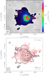 |
Fig. 1 Top panel: 1.3 mm ALMA continuum emission map of the HMC G31. The contours are 5, 10, 15, 20, 40, 80, 160, and 300 times σ, where 1σ is 1.2 mJy beam−1. The white dots mark the position of four embedded continuum sources observed at 1.4 mm and 3.5 mm (Beltrán et al., in prep.). The red cross indicates the position of the UC H II region imaged by Cesaroni et al. (1994). The synthesized beam is shown in the lower left-hand corner. Bottom panel: magnetic field segments (red lines), obtained by rotating 90° the polarization segments, overlapped on the 1.3 mm continuum emission map (contours). The segments are sampled following Nyquist sampling (every five pixels). |
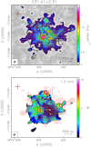 |
Fig. 2 Top panel: linearly polarized intensity P (colors) and dust continuum emission map (contours) at 1.3 mm in G31. Polarized intensity ranges from 0.11 to 2.4 mJy beam−1. Bottom panel: polarization fraction p (colors) anddust continuum emission map (contours) at 1.3 mm. Polarization fraction ranges from 0.1 to 13%. The red thick segments in both panels indicate the magnetic field lines. Segments are shown every eight pixels. The synthesized beam is shown in the lower left-hand corner. Contours and symbols are the same as in Fig. 1. |
4 Analysis
4.1 Modeling the magnetic field
Assuming that the polarization pattern is due to dust grains with their shortest axis aligned to the magnetic field, we used the DustPol module of the ARTIST package (Padovani et al. 2012) to model the magnetic field morphology. We modeled G31 as an axially-symmetric singular toroid threaded by a poloidal magnetic field (Li & Shu 1996; Padovani & Galli 2011). Following Padovani et al. (2013), we added a toroidal force-free component of the magnetic field, modified here to mimic the effects of rotation. In practice, we allowed the magnetic field to make a “kink” at the midplane, assuming opposite signs of the toroidal component above and below the midplane. The ratio of the toroidal and poloidal components of the field remains approximately constant along each field line, except close to the magnetic axis, which coincides with the rotation axis, where the toroidal component dominates (see Padovani et al. 2013 for details).
This model has four free parameters: (i) the mass-to-flux ratio, λ, defined as
 (1)
(1)
where G is the gravitational constant, Φ the magnetic flux, and M(Φ) the mass contained in the flux tube Φ; (ii) the ratiob0 between thestrength of the toroidal and the poloidal components of the magnetic field in the midplane of the source; (iii) the orientation of the projection of the magnetic axis on the plane of the sky, φ, measured from north to east (i.e., counterclockwise); and (iv) the inclination with respect to the plane of the sky, i, assumed to be positive (negative) if the magnetic field in the northern sector points toward (away from) the observer. The model is isothermal, and the value of the soundspeed provides the scaling for both the density and the magnetic field strength. In order to match the observed intensity at 1′′, we set the effective sound speed to 1.4 km s−1.
We considered three different values for the mass-to-flux ratio, which controls the pinching of the field lines as well as the flatness of the density distribution: λ = 1.63, corresponding to the case of strong field and flat density profile, λ = 8.38, corresponding to the case of weak field and quasi-spherical density profile, and an intermediate case, λ = 2.66 (see Table 1 of Li & Shu 1996). We also accounted for different values of b0, ranging from the purely poloidal case (b0 = 0) to the case where the toroidal component is half of the poloidal component in the midplane (b0 = 0.5). We assumed the temperature profile modeled by BEL18, and we verified a posteriori that using a constant temperature does not significantly affect our conclusions (see Sect. 4.2).
The DustPol module is an extension to the Line Modeling Engine (LIME) radiative transfer code (Brinch & Hogerheijde 2010). Besides calculating line profiles in the far infrared and submillimeter regimes, LIME can ray-trace given density and temperature profiles, estimating the continuum flux. DustPol computes the Stokes I, Q, and U maps (see Eqs. (4)–(8) in Padovani et al. 2012) and stores them in FITS format, which are straightforwardly used as an input for the tasks simobserve and simanalyze of CASA, adopting the same antenna configuration of the observing runs. Finally, from these synthetic maps we generated the polarization angle patterns to be compared with those obtained from the observations. For each combination of λ, b0, φ, and i, we performed a chi-squared test for the difference between the observed and the modeled polarization angles within the 5σ contour of the 1.3 mm dust emission map. We found that the polarization pattern is in general well reproduced by a purely poloidal magnetic field. Adding a small toroidal component slightly improves the quality of the fit, provided the latter is not larger than ~10% of the poloidal component (see Appendix B). Therefore, from now on, we only consider the case b0 = 0.1 in our models. For the sake of completeness, Appendix B shows the results of our modeling for b0 = 0, 0.25, and 0.5.
Figure 3 shows the reduced chi squared3,  , as a function of the inclination, i, and the orientation, φ, for b0 = 0.1 and the three values of λ. The high values of
  are due to the very low average value of the uncertainty on the observed polarization angle, δψobs, which is less than about 4° inside the 5σ contour of the 1.3 mm dust continuum emission. In contrast, the polarization angle residuals, Δψ = ψobs − ψmod, given by the difference between the observed(ψobs) and modeled (ψmod) polarization angles for the best model, can be as large as ±90°, because the model does not include the turbulent component of the magnetic field (see Sect. 4.2 and Appendix A for details).
Independently of the value of λ, all the curves show a minimum around φ ~ −45°, but the higher the mass-to-flux ratio, the lower is the difference in  between positive andnegative inclinations. This is explained by the fact that on the one hand the difference between negative and positive inclinations is significant only for large opacities; on the other hand, a large mass-to-flux ratio corresponds to a less centrally-condensed source, which is more optically thin. We verified this statement using DustPol, which also calculates the dust opacity, τ, and the values obtained for mass-to-flux ratios of 1.63, 2.66, and 8.38 at the density peak are 1.1, 0.8, and 0.6, respectively. This allowed us to discard the case λ = 8.38, since we know that G31 is optically thick toward the center (BEL18). We found that the best model is given by λ = 2.66,
  , and
, and  . The 1σ errors have been estimated using the method of Lampton et al. (1976).
Figure 4 shows the comparison between the polarization angles obtained from observations and those from the best fit model. Even if the overall result is consistent with our best model, we remark that there are a few regions showing departures from this geometry (see Fig. 5): (i) the center of the Main core where there are four embedded sources (see Fig. 1) and we may expect a more complex configuration of the magnetic field lines; (ii) the NE core, where the magnetic field appears to show an independent poloidal configuration inside a radius of ≲ 0.5′′ probably due to its own collapse; and (iii) the northern and southwestern edges of the Main core, where two different molecular outflows have been traced in SiO (BEL18). See Sect. 5 for a detailed discussion on the possible causes of the deviation.
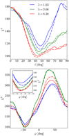 |
Fig. 3 Top panel: minimum reduced chi squared versus the inclination, i, of the model for three different values of the mass-to-flux ratio, λ, and b0 = 0.1. Solid (dashed) lines show |


4.2 Magnetic field strength estimate
Now, we take advantage of our model fit to measure the magnetic field strength using the Davis–Chandrasekhar–Fermi method (Davis 1951; Chandrasekhar & Fermi 1953). For this purpose, it is necessary to estimate the dispersion of the polarization angle with respect to the model. We thus computed the histogram of the polarization angle residuals. We considered the region inside the 15σ contour level to focus only on the Main core, avoiding any contamination by the NE core. The average uncertainty on the observed polarization angles is  , where σQU = 22 μJy beam−1 is the noise on the observed Stokes Q and U. This expression is valid for high (>5) signal-to-noise ratios (S/N) (e.g., Vaillancourt 2006), which is the case of our data. As seen in Fig. 2 (top panel), the linearly polarized intensity, P, of the G31 core is > 5σQU. In the region inside the 15σ contour of the 1.3 mm dust continuum map, δψobs ≲ 2° (see Fig. A.1), therefore, we used a histogram bin of 4°.
Figure 6 shows the distribution of polarization angle residuals for our best model. A Gaussian fit over the whole distribution of residuals gives an average value of 0.6° ± 27.6°. As shown in this figure, the polarization angle residuals can be very large, up to ± 90°. To better discriminate the areas with large dispersion, we plotted in Fig. 7 the polarization angle residuals over the whole G31 core. This figure shows that the residuals Δψ in the Main core (inside the 15σ contour level) are between − 45° and 45° except for small areas associated with the four embedded sources or in the direction of the NE core and the north–south (N–S) outflow mapped in SiO by BEL18. As already mentioned in the previous section, these regions will be analyzed in detail in Sect. 5 and the possible causes of the large deviations from the model will be discussed. Therefore, assuming that these high dispersion values indicate areas where the initial magnetic field associated with the Main core has been disturbed, we decided to limit the range of Δψ between − 45° and + 45°. In this case, the average value of the distribution of residuals is 2.3° ± 17.3°. Therefore, the standard deviations on the polarization angle dispersion from the two Gaussian fits, σψ, are 27.6° and 17.3°. If in our model we adopt a constant temperature of 250 K, which is the mean value in the G31 Main core (BEL18), the average value of the distribution of residuals is 2.6° ± 30.2°, considering the whole angle distribution, and 5.1° ± 16.9°, if limited in the range ±45°. Therefore, the difference between the average values of the distributions of residuals in the isothermal and non-isothermal cases is not significant. Since the measurement uncertainty of the polarization angle δψobs is ≲ 2°, the intrinsic dispersion is δψint =  .
.
To estimate the strength of the magnetic field on the plane of the sky, Bpos, we used the Davis–Chandrasekhar–Fermi method, which is based on the assumption that the perturbations responsible for the polarization angle dispersion δψint are Alfvén waves of amplitude  , where ρ is the density and σlos is the line-of-sight velocity dispersion. This gives
 (2)
(2)
where ξ = 0.5 is a correction factor derived from turbulent cloud simulations (Ostriker et al. 2001). The line-of-sight velocity dispersion σlos has been computed from the line width ΔV of the CH3CN observationsof BEL18, which have an angular resolution similar to that of our polarization observations, as  . To avoid the effects of rotation on the line broadening, we estimated ΔV at different pixel positions of the core and then averaged the values. The thermal contribution to the velocity dispersion is negligible for the temperatures ≳100 K estimated for the Main core (e.g., BEL18). Using ΔV ≃ 5 km s−1, the value of σlos is 2.1 km s−1. This value is consistent with the turbulent velocity dispersion of 2.7 km s−1 obtained by Osorio et al. (2009) from the modeling of the G31 core. The average volume density of the Main core has been computed assuming spherical symmetry from the mass estimate of BEL18, which has been computed for a radius, R, of 1′′. 1. This radius corresponds to that of the Main core inside the 15σ contour level (see Fig. 1). We note that the mass of 120 M⊙ of BEL18 was estimated for a distance of 7.9 kpc. Assuming a distance of 3.7 kpc, the mass of the Main core is ~26 M⊙ and the corresponding mean number density is n = 1.4 × 107 cm−3. Our modeling provides the inclination with respect to the plane of the sky, i, which allows us to estimate the total magnetic field strength as B = Bpos∕ cosi ≃ 8–13 mG, for an intrinsic dispersion of 27.6° and 17.3°, respectively. GIR09 have estimated a value of Bpos of ~ 14 mG (corrected for a distance of 3.7 kpc), that for the inclination angle of − 45° derived from our modeling, corresponds to a strength of the magnetic field of ~ 20 mG, slightly higher than our estimate. This result is consistent with the range of magnetic field strengths predicted by the model (12 mG at 0′′. 2 and 3 mG at 1′′, see Fig. 8).
Finally, we evaluated the mass-to-flux ratio from Eq. (1) to check the consistency of our model (with λ > 1, “supercritical”) with the observations. We computed the magnetic flux, Φ = πR2B, inside a radius of 1′′.1, corresponding to the Main core region, assuming spherical symmetry, and obtained a range of (0.9–1.5) × 1032 G cm2. As for M(Φ), the mass contained in the flux tube Φ, we assumed that this is the mass of the core (26 M⊙) plus the mass of the (proto)stars already formed in the core. We estimated the mass of the (proto)stars from the bolometric luminosity of the region, which is ~ 4.4 × 10⁴ L⊙. If we assume that the bolometric luminosity of the core is mainly produced by a single main-sequence star, then the mass of such star would be of ~20 M⊙, corresponding to an O8.5–O9 star (Mottram et al. 2011). Consequently, M(Φ) = 46M⊙ and λ lies in the range 1.0–1.6. Thedefinition of λ in Eq. (1) accounts for the mass inside a flux tube, while from observations we estimated the mass in a sphere of radius 1.1′′. We then multiply the latter by a correcting factor equal to 1.4 (Li & Shu 1996) to obtain λ ~ 1.4–2.2, slightly supercritical. We note that the observed value of the mass-to-flux ratio should be taken as a lower limit because the mass of the core should be taken as a lower limit and the stellar mass content could be larger if the luminosity of 4.4 × 10⁴ L⊙ originates from multiple stars instead of a single star as previously assumed by us. In addition, Estalella et al. (2019) have recently modeled theline-of-sight velocity of ammonia as a function of projected distance in the G31 core and have obtained a central mass ≳44 M⊙. Therefore, we believe that the mass-to-flux ratio computed from the observations is consistent with λ = 2.66 assumed for the model.
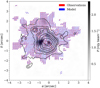 |
Fig. 4 Polarization angles showing the magnetic field direction from observations (red) and the best model (blue: b0 = 0.1, λ = 2.66, |


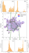 |
Fig. 5 Middle plot: comparison between the observed and the modeled polarization angles superposed to the contours of the 1.3 mm dust continuum emission (see Fig. 4 for details). The four histograms show the polarization angle residuals for the NE core (a), and for the regions associated with two of the outflows mapped in SiO in the core: that associated with the N–S outflow located to the north of the Main core (b), and those associated with the E–W outflow to the southeast (c) and southwest (d) of the Main core (see Sect. 5.4). For the latter regions (b–d), the histograms of the polarization angle residuals have been calculated in the regions encompassing the 5 and 15σ contours. |
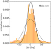 |
Fig. 6 Histogram of the polarization angle residuals for our best model in the region inside the 15σ contour (corresponding to the Main core) of the 1.3 mm dust continuum map. The dashed and solid black lines show two Gaussian fits obtained considering the whole range of Δψ and limited to ±45°, respectively. |
 |
Fig. 7 Polarization angle residuals (color map) superposed the 1.3 mm dust continuum emission contours (gray solid lines). The black dots mark the position of four embedded continuum sources (see Fig. 1). Blue and red contours show the regions where Δψ > 45° and < −45°, respectively.Dashed gray lines indicate the direction of the E–W and N–S outflows mapped in SiO by BEL18. |
5 Discussion
5.1 A supercritical core
The mass-to-flux ratio of λ > 1.4 obtained by us with a beam of 0′′. 2 is consistent with the value of ~1.8 estimated by GIR09 with 1″ resolution, after correcting for the new 3.7 kpc distance. We note, however, that GIR09 used Bpos to estimate λ. Using the value of B (assuming an inclination angle of − 45°), the mass-to-flux ratio estimated from the 870 μm dust emission would be 1.3. The estimated mass-to-flux ratio suggests that the G31 core is slightly supercritical at different scales, from ~800 to ~4000 au. This is further supported by the detection of signatures of infall, such as red-shifted absorption and a central spot of blue-shifted emission (GIR09; Mayen-Gijon et al. 2014; BEL18; Estalella et al. 2019), and by the presence of at least four embedded sources in the Main core. We estimated the Alfvén velocity from the expression4  . Using the estimates of the magnetic field strength in G31, we obtain an Alfvén velocity in the range 3–5 km s−1. These values are comparable to, or slightly lower than, the infall velocities estimated by BEL18 from red-shifted absorption (~ 2–8 km s−1). The highest infall velocities have been estimated for the vibrationally excited transitions of CH3CN and for some transitions of the isotopologues 13CH3CN and CH
 CN, which are optically thinner and trace material close to the central (proto)star(s). Therefore, this suggests that while the collapse in the external part of the core is slightly sub-Alfvénic, it becomes super-Alfvénic close to the center.
The Davis–Chandrasekhar–Fermi method also allows to estimate the ratio of the turbulent component of the magnetic field,  , to the uniform component B = Bpos∕ cosi. With Bpos given by Eq. (2), this ratio results
![Mathematical equation: \begin{eqnarray*} \frac{\delta B}{B}\,{\sim}\,\frac{\sqrt{3}\cos i}{\xi}\delta\psi_{\textrm{int}}. \\[-13pt] \nonumber \end{eqnarray*}](/articles/aa/full_html/2019/10/aa35701-19/aa35701-19-eq17.png) (3)
(3)
Inserting the numerical values, we obtain δB∕B ~ 0.7 and ~ 1, for δψ = 17.3° and 27.6°, respectively. This indicates that the energy of the turbulent component of the magnetic field in the Main core of G31 is a significant fraction (50% or larger) of the energy of the uniform component of the field included in our model.
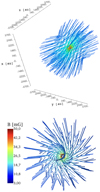 |
Fig. 8 Upperpanel: magnetic field configuration inside a radius of 3700 au, corresponding to the radius of the Main core in G31, for b0 = 0.1, i = − 45°, and φ = −44°. Lower panel:magnetic field line configuration for b0 = 0.1 shown almost pole-on to emphasize the line twisting close to the symmetry axis. The spatial scale is the same in both panels (the model extends up to a radius of 3700 au). The color of the magnetic field lines indicates the magnetic field strength in both panels (see color scale in the bottom panel). |
5.2 Confirming the rotating toroid model
Molecular line observations have revealed a striking northeast-southwest (NE–SW) velocity gradient in the G31 core on scales from 103 –104 au (Beltrán et al. 2004, 2005, BEL18; Araya et al. 2008; GIR09; Cesaroni et al. 2011). The interpretation of this NE–SW velocity gradient has been long controversial. Some authors (Beltrán et al. 2004, 2005, BEL18; GIR09; Cesaroni et al. 2011) propose that the velocity gradient is produced by the rotation of the core. In contrast, Araya et al. (2008) interpret such a gradient as due to a compact bipolar outflow. Our model fit allows us for the first time to discriminate between both scenarios.
The position angle of the magnetic axis, φ, is probably the quantity better constrained by the fitting procedure, because as already mentioned in Sect. 4.1, independent of the mass-to-flux ratio of the model, the symmetry axis of the hourglass B field is oriented SE–NW, with φ approximately − 45°. This orientation is almost perpendicular to the NE–SW velocity gradient and to the main axis of the core dust continuum emission (BEL18). In addition, as shown in Fig. 3, the chi-squared function is maximum at ~ 40°, which suggests that this direction is the most unlikely for the magnetic field. This result points to the fact that the magnetic field is oriented perpendicular to the plane of the core and almost parallel to the rotation axis. This is important because it supports the hypothesis that the velocity gradient is due to rotation and discards the molecular outflow scenario proposed by Araya et al. (2008).
5.3 Influence of rotation on the magnetic field
The angular velocity Ω of the rotation of the G31 core has been estimated by BEL18 for different transitions with different energies of CH3CN and its isotopologues and is Ω = (2.7–5.4) × 10−12 s−1 for a radius of 3700 au, depending on the transition. This rotation appears to have little effect on the magnetic field, as suggested by the modeling (see Fig. 8). In fact, as seen in Sect. 4.1, we find that the magnetic field geometry in G31 is well represented by a toroidal component not larger than 10% of the poloidal component. A similar behavior has been observed in the low-mass systems BHB07-11 (Alves et al. 2018) and VLA 1623-A in Ophiuchus (Savadoy et al. 2018), despite the differentspatial scales and associated protostellar masses. In any case, we stress that, as shown in Fig. 8, the direction of rotation of the modeled toroidal component coincides with that of the core, which rotates clockwise.
A possible explanation for the fact that rotation does not seem to affect the magnetic field could be a decoupling of the envelope and the magnetic field. A partial decoupling could be produced by several causes, for example: the removal by coagulation of very small charged grains, with size ~ 10−2 μm, that dominate the coupling of the bulk neutral matter to the magnetic field (Zhao et al. 2016); or an attenuation of the flux of ionizing cosmic-ray particles expected in the dense regions around a forming protostar (Padovani et al. 2014, 2018). Another possibility to explain such a small toroidal component could be that the core is still young and therefore rotation had no time to affect the magnetic field yet. Starting from a purely poloidal magnetic field, a rotation of the core of an angle of ~ π∕2, occurring on a timescale on the order of π∕(2Ω) = (1.0–2.0) × 104 yr, would generate in the source’s midplane a field with toroidal-to-poloidal intensity ratio b0 ~ 1. Thus, if the magnetic field and the envelope are well coupled, the value of b0 ≲ 0.1 resulting from our modeling would imply an “age” of a few 103 yr, suggesting that the G31 core is very young.
5.4 Perturbation of the magnetic field
The polarized emission in G31 has been successfully fit with a semi-analytical magnetostatic model of a toroid supported by magnetic fields. As seen in the previous section, the magnetic field associated with G31 Main core is basically poloidal. This almost poloidal model fits the observed magnetic field lines in most of the core extremely well but it deviates from the observations in some areas. Figures 5 and 7 show that our model fails to properly describe the magnetic field close to the center of the Main core, around the NE core, and at the northern and southwestern edges of the Main core. In the next sections, we discuss the possible causes of the large deviations from the model in these areas.
5.4.1 The central region
As shown in Fig. 7, the discrepancies between the observed and predicted polarization angles are large close to the center of the Main core, and in particular at the position of the four embedded sources (see Sect. 3.1). The dispersion in the residuals in this area is large (|Δψ| > 45°), compared to the average values in the Main core. The presence of the embedded sources indicates that fragmentation has already taken place in the core. Therefore, this suggests that, despite its strength (~10 mG), the magnetic field is not sufficient to prevent the fragmentation and collapse of the core.
The embedded sources appear to be in the accretion phase, as suggested by the detection of red-shifted absorption toward them (Beltrán et al., in prep.). Therefore, the existence of different collapsing centers that might drag and perturb the larger-scale magnetic field makes it very difficult to model the magnetic field in such environment with our idealized model. This could explain the large polarization angles residuals toward the embedded sources at the center of the Main core.
5.4.2 The NE core
Albeit smaller and weaker than the Main core, the NE core is also a HMC, as indicated by the detection of several transitions of methyl cyanide and methyl formate (see Fig. A.1 of BEL18). The magnetic field toward this core is strongly disturbed and cannot be properly fit with our model (see Fig. 5). The polarization angle residuals are large (|Δψ| > 45°) (Fig. 7). As shown in Fig. 1, the observed magnetic field at the position of the NE core, in particular to the northeast of the core, appears to show an independent poloidal configuration (hourglass shape) that could be produced by gravitational collapse. If we assume a dust temperature of 50–100 K, consistent with the fact that the NE core is a HMC, we obtain a mass of the core MNE ≃ 3–6.5 M⊙, for an integrated flux density of 52 mJy (BEL18), a dust absorption coefficient per unit mass κν = 0.008 cm2 g−1 at 217 GHz (Ossenkopf & Henning 1994), and a gas-to-dust mass ratio of 100.
In this scenario, the magnetic field lines are dragged to the center ofcollapse associated with the NE core and perturb the magnetic field associated with the Main core. In our model, the magnetic field is associatedand centered with the Main core, and therefore, we cannot reproduce the perturbations resulting from the collapse of the NE core.
The large-scale magnetic field, to the north and to the east of the position of the NE core (see Figs. 4 and 5), also follows an hourglass morphology which could indicate the presence of a filament channeling mass inflow to the center of the G31 core where NE and Main are embedded.
5.4.3 The molecular outflows
The 870 μm SMA polarized observations by GIR09 revealed a clear lack of polarized emission to the west of the core dust continuum emission peak (see their Fig. 1A). Our ALMA observations have confirmed this lack of polarized emission, and have better pinpointed its location at the southwestern edge of the Main core (Fig. 2; top panel). This unpolarized region appears to coincide with the blue-shifted, western lobe of an SiO molecular outflow (the E–W outflow mapped by BEL18; see Fig. 9). This outflow is centered ~0′′.6 to the south of the dust continuum emission peak and could be associated with the southernmost of the four embedded sources. The polarized emission also seems to surround the red-shifted lobe of this outflow to the east (Fig. 9). In both cases, the polarized emission traces the walls of the cavities opened by the outflow. The fact that there is no polarized emission along most of the molecular outflow could be due to the lack of dust, which might have been evacuated by the outflow. This has also been observed in low- and intermediate-mass protostars (e.g., Serpens SMM1: Hull et al. 2017b; B335: Maury et al. 2018). In some cases the polarization is enhanced along the walls of the outflow cavity (e.g., B335: Maury et al. (2018); Ser-emb 8(N): Hull et al., in prep.). This polarization enhancement is also marginally observed in G31 (see Fig. 2). All this has led to suggestions that the outflow might shape the magnetic field (Hull et al. 2017b). One expects that the outflow sweeps away the core material, thereby creating heated and compressed regions at its edges, and it is in these regions that the magnetic field is disturbed.
In fact, this effect is observed in G31. The magnetic field at the base and along the walls of the E–W outflow cavities is partially perturbed. As shown in Fig. 7, |Δψ| < 30° except for localized regions. This is especially true for the northern part of the blue-shifted, western lobe and the southern part of the red-shifted, eastern lobe. We speculate that the perturbed field is detected in regions where there is no significant dust emission from the core along the line-of-sight or this component has been filtered out by the interferometer.
The other effect of the molecular outflow is that, by generating an almost dust free cavity, the photons from the inner regions around the protostar can more easily escape from the core, illuminating the cavity. This could enhance the polarization efficiency through radiative torques (Hoang & Lazariano 2009; Andersson et al. 2015). There is some evidence of higher polarization degree in the northern part of the blue-shifted, western lobe. In addition, the red-shifted eastern lobe shows polarization where no Stokes I emission is detected, which also may indicate an enhancement of the polarization. That only Stokes Q and U emission is detected in the red-shifted eastern lobe is due to the sensitivity of the maps, because while the rms noise of the maps for Stokes Q and U is 22 μJy beam−1, that for Stokes I is a factor 55 higher (1.2 mJy beam−1).
BEL18 have also mapped a N–S SiO molecular outflow in the region, which is hardly visible in Fig. 9. This outflow, which is much weaker than the east-west one, could be driven by one of the embedded centimeter continuum sources detected by Cesaroni et al. (2010) at the center of the Main core. Despite the fact that this outflow has not yet excavated wide cavities, it appears to have strongly disturbed the magnetic field at the northern edge of the Main core. As shown in Figs. 5 and 7, the observed and modeled polarization angles strongly diverge to the north and the polarization angle residuals arealways larger than 30°.
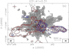 |
Fig. 9 Overlay of the blue-shifted (blue contours) and red-shifted (red contours) SiO (5–4) averaged emission from BEL18 on the polarized intensity map (gray scale). The blue-shifted and red-shifted emission have been averaged over the (73, 90) km s−1 and (103, 119) km s−1 velocity interval, respectively. Contour levels are 3, 6, 12, and 24 times 1.1 mJy beam−1. Gray-scale contours for the polarized intensity are 5, 10, 50, and 90 times σ, where 1σ is 22 μJy beam−1. The white segments, plotted every ten pixels, indicate the magnetic field lines. White dots mark the position of the four embedded continuum sources (Beltrán et al., in prep.). Dashed black lines indicate the direction of the E–W and N–S outflows mapped in SiO by BEL18. The synthesized beam of the polarized emission and of the SiO observations are shown in the lower left-hand and lower right-hand corner, respectively. |
5.5 Comparison with other regions
The direct face to face comparison between the dust polarization pattern and theoretical predictions of the collapse of a magnetized dense core can basically be done when the observed magnetic field morphology resembles relatively simple magnetic field poloidal, toroidal configuration, or a combination of them (e.g., Gonçalves et al. 2008; Alves et al. 2018). This is the case for the two well known low- and high-mass star-forming cores, G31 and NGC 1333 IRAS 4A (Frau et al. 2011 and this work). Interestingly, the two cores present a velocity gradient almost perpendicular to the main direction of the magnetic field (Beltrán et al. 2005; Ching et al. 2016), but the field lines appear not to be perturbed by the rotation. Of these two cores, G31 appears to have the mass-to-flux ratio closest to the critical value.
The hourglass morphology has also been reported in other massive cores (Schleuning et al. 1998; Qiu et al. 2014; Li et al. 2015), and in low-mass cores (Girart et al. 1999, 2006; Davidson et al. 2014; Kwon et al. 2019; Maury et al. 2018). These are clear cases of magnetically regulated star formation with a relatively uniform magnetic field at core and/or envelope scales. However, there are other cases reported in the literature that indicate the opposite, namely that the magnetic field plays a minor role in the star-formation process. In some cases, the magnetic field appears to be affected by the stellar feedback (Tang et al. 2009, 2010; Frau et al. 2014), but in other cases, the magnetic field appears to be weak energetically with respect to turbulence, angular momentum and/or gravity (Girart et al. 2013; Hull et al. 2017a; Cortes et al. 2016; Juárez et al. 2017). This suggests that there is a diverse initial condition at the onset of gravitational collapse. Statistically, polarization observations with single-dish telescopes of a significant sample of star-forming clouds found a significant fraction of sources for which the magnetic field appears to be relevant (Koch et al. 2014). Probing similar spatial scales as in this study of G31, Zhang et al. (2014) presented polarization studies of 14 massive molecular clumps with the SMA. By comparing with magnetic field orientations at the parsec scale, they found that the field in dense cores is correlated with that in their parental clumps, thus, concluded on a statistical basis that magnetic fields are dynamically important in shaping the fragmentation of the parsec-scale clumps and the formation of dense molecular cores. Furthermore, they found no strong correlation between the core magnetic field orientation and the major axis of molecular outflows (see also Hull et al. 2013; Galametz et al. 2018), which suggests that the role of magnetic fields are weakened relative to gravity and angular momentum at scales from cores to accretion disks. In comparison to these statistical studies, G31 represents a case that magnetic fields are dynamically dominant at scales of dense cores, and maintain the importance down to the scale of 103 au. As discussed in Hull & Zhang (2019), this hourglass-shaped magnetic field configuration is relatively rare in both high-mass and low-mass star forming cores.
6 Conclusions
We carried out ALMA 1.3 mm high-angular (~0′′.2) resolution polarization observations of the hot molecular core G31.41+0.31, previously observed with the SMA at 870 μm with lower (~1″) angular resolution. The ALMA observations have confirmed the hourglass-shaped magnetic field morphology observed previously with the SMA.
The polarization fraction in the HMC ranges from 0.1 to 13%. However, these values should be taken as lower limits due to the fact that at least ~40% of the total flux measured for Stokes I is contaminated by line emission.
The polarized emission in the central region of G31 has been successfully fit with a semi-analytical magnetostatic model of a toroid supported by magnetic fields. The best fit model suggests that the magnetic field associated with the Main core in G31 is well represented by a purely poloidal field, with a possible hint of a toroidal component on the order of 10% of the poloidal component (b0 ≤ 0.1), that is oriented SE–NW (position angle  ) and has an inclination
  , for a mass-to-fluxratio λ = 2.66. The magnetic field is oriented perpendicular to the NE–SW velocity gradient detected in this core on scales from ~103 to 104 au consistent with our previous hypothesis that such a velocity gradient is due to rotation of the core.
The almost poloidal geometry of the magnetic field in G31 is only perturbed by the collapse of both the Main core and the NE core, and by the molecular outflows detected in the core. Notwithstanding the rotation of the core, this appears to have little effect on the magnetic field, as suggested by the fact that the best fit model includes only a very small toroidal component.
The strength of the magnetic field in the central region of the core has been estimated using the Davis–Chandrasekhar–Fermi method and is in the range ~8 to 13 mG. This strength implies that the mass-to-flux ratio in this region is only slightly supercritical (λ = 1.4–2.2). In fact, despite the magnetic field being important in G31, it is not sufficient to prevent fragmentation and collapse of the core, as demonstrated by the presence of (at least) four sources embedded in the Main core. The turbulent-to-magnetic energy ratio suggests that the two are comparable.
Acknowledgements
We thank the anonymous referee and Philip Myers for their useful comments that have improved the manuscript. This paper makes use of the ALMA data ADS/JAO.ALMA#2015.1.00072.S. ALMA is a partnership of ESO (representing its member states), NSF (USA) and NINS (Japan), together with NRC (Canada) and NSC and ASIAA (Taiwan) and KASI (Republic of Korea), in cooperation with the Republic of Chile. The Joint ALMA Observatory is operated by ESO, AUI/NRAOand NAOJ. M.P. acknowledges funding from the European Unions Horizon 2020 research and innovation programme under the Marie Skłodowska-Curie grant agreement No 664931. J.M.G. acknowledges support from MICINN (Spain) AYA2017-84390-C2-2-R grant. G.A. and M.O. acknowledge financial support from the State Agency for Research of the Spanish MCIU through the AYA2017-84390-C2-1-R grant (co-funded by FEDER) and through the “Center of Excellence Severo Ochoa” award for the Instituto de Astrofísica de Andalucía (SEV-2017-0709).
Appendix A: Error on the observed polarization angles
The error on the polarization angle is computed by propagating the error from the definition of ψ (see Sect. 2) and it is equal to  , where σQU = 22 μJy is the noise on the observed Stokes Q and U. This expression of uncertainty in the polarization angle is valid for high (> 5) S/N (e.g., Vaillancourt 2006), which is the case of our data. As seen in Fig. 2 (top panel), the linearly polarized intensity P of the G31 core is > 5σQU. Figure A.1 shows that δψobs is lower than about 4° inside the 5σ contour of the 1.3 mm dust continuum emission and, on average, is lower than 2° inside the 15σ contour encompassing the Main core.
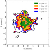 |
Fig. A.1 Map of the errors on the observed polarization angles according to the color-coding shown in the legend. Black contours show the 5σ and 15σ levels of the 1.3 mm dust continuum emission. White regions inside the 5σ contour referto δψobs ≥ 4°. |
Appendix B: Chi-squared test for different values of the toroidal component
Figure B.1 shows the values of  as a function of the inclination for different values of b0. This test allowed us to discard the cases with b0 > 0.1.
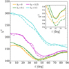 |
Fig. B.1 Minimum reduced chi squared versus the inclination, i, of the model for λ = 2.66 and increasing toroidal component. Solid (dashed) lines show |


References
- Alves, F. O., Girart, J. M., Padovani, M., et al. 2018, A&A, 616, A56 [NASA ADS] [CrossRef] [EDP Sciences] [Google Scholar]
- Andersson, B.-G., Lazarian, A., & Vaillancourt, J. E. 2015, ARA&A, 53, 501 [NASA ADS] [CrossRef] [Google Scholar]
- Araya, E., Hofner, P., Kurtz, S., Olmi, L., & Linz, H. 2008, ApJ, 675, 420 [NASA ADS] [CrossRef] [Google Scholar]
- Bacciotti, F., Girart, J. M., Padovani, M., et al. 2018, ApJ, 865, L12 [NASA ADS] [CrossRef] [Google Scholar]
- Basu, S., & Mouschovias, T. Ch. 1994, ApJ, 432, 720 [NASA ADS] [CrossRef] [Google Scholar]
- Beltrán, M. T., Cesaroni, R., Neri, R. et al. 2004, ApJ, 601, L190 [Google Scholar]
- Beltrán, M. T., Cesaroni, R., Neri, R., et al. 2005, A&A, 435, 901 [NASA ADS] [CrossRef] [EDP Sciences] [Google Scholar]
- Beltrán, M. T., Cesaroni, R., Rivilla, V. M., et al. 2018, A&A, 615, A141 [NASA ADS] [CrossRef] [EDP Sciences] [Google Scholar]
- Brinch, C., & Hogerheijde, M. 2010, A&A, 523, A25 [NASA ADS] [CrossRef] [EDP Sciences] [Google Scholar]
- Cesaroni, R., Churchwell, E., Hofner, P., Walmsley, C. M., & Kurtz, S. 1994, A&A, 288, 903 [NASA ADS] [Google Scholar]
- Cesaroni, R., Hofner, P., Araya, E., & Kurtz, S. 2010, A&A, 590, A50 [NASA ADS] [CrossRef] [EDP Sciences] [Google Scholar]
- Cesaroni, R., Beltrán, M. T., Zhang, Q., Beuther, H., & Fallscheer, C. 2011, A&A, 533, A73 [NASA ADS] [CrossRef] [EDP Sciences] [Google Scholar]
- Chandrasekhar, S., & Fermi, E. 1953, ApJ, 118, 113 [NASA ADS] [CrossRef] [Google Scholar]
- Ching, T.-C., Lai, S.-P., Zhang, Q., et al. 2016, ApJ, 819, 159 [NASA ADS] [CrossRef] [Google Scholar]
- Cortes, P. C., Girart, J. M., Hull, C. L. H., et al. 2016, ApJ, 825, L15 [NASA ADS] [CrossRef] [Google Scholar]
- Davidson, J. A., Novak, G., Matthews, T. G., et al. 2011, ApJ, 732, 97 [NASA ADS] [CrossRef] [Google Scholar]
- Davidson, J. A., Li, Z.-Y., Hull, C. L. H., et al. 2014, ApJ, 797, 74 [NASA ADS] [CrossRef] [Google Scholar]
- Davis, L. 1951, Phys. Rev. 81, 890 [NASA ADS] [CrossRef] [PubMed] [Google Scholar]
- Dent, W. R. F., Pinte, C., Cortes, P. C., et al. 2018, MNRAS, 482, L29 [Google Scholar]
- Estalella, R., Anglada, G., Díaz-Rodríguez, A. K., & Mayen-Gijon, J. M. 2019, A&A, 626, A84 [NASA ADS] [CrossRef] [EDP Sciences] [Google Scholar]
- Fiedler, R. A., & Mouschovias, T. Ch. 1993, ApJ, 415, 680 [NASA ADS] [CrossRef] [Google Scholar]
- Frau, P., Galli, D., & Girart, J. M. 2011, A&A, 535, A44 [NASA ADS] [CrossRef] [EDP Sciences] [Google Scholar]
- Frau, P., Girart, J. M., Zhang, Q., & Rao, R. 2014, A&A, 567, A116 [NASA ADS] [CrossRef] [EDP Sciences] [Google Scholar]
- Galametz, M., Maury, A., Girart, J. M., et al. 2018, A&A, 616, A139 [NASA ADS] [CrossRef] [EDP Sciences] [Google Scholar]
- Galli, D., & Shu, F. H. 1993a, ApJ, 417, 220 [NASA ADS] [CrossRef] [Google Scholar]
- Galli, D., & Shu, F. H. 1993b, ApJ, 417, 243 [NASA ADS] [CrossRef] [Google Scholar]
- Galli, D., Lizano, S., Shu, F. H., & Allen, A. 2006, ApJ, 647, 374 [NASA ADS] [CrossRef] [Google Scholar]
- Girart, J. M., Crutcher, R. M., & Rao, R. 1999, ApJ, 525, L109 [NASA ADS] [CrossRef] [Google Scholar]
- Girart, J. M., Rao, R., & Marrone, D. P. 2006, Science, 313, 812 [NASA ADS] [CrossRef] [PubMed] [Google Scholar]
- Girart, J. M., Beltrán, M. T., Zhang, Q., Rao, R., & Estalella, R. 2009, Science, 324, 1408 [NASA ADS] [CrossRef] [PubMed] [Google Scholar]
- Girart, J. M., Frau, P., Zhang, Q., et al. 2013, ApJ, 772, 69 [NASA ADS] [CrossRef] [Google Scholar]
- Girart, J. M., Fernández-López, M., Li, Z.-Y., et al. 2018, ApJ, 856, L27 [CrossRef] [Google Scholar]
- Gonçalves, J., Galli, D., & Girart, J. M. 2008, A&A, 490, L39 [NASA ADS] [CrossRef] [EDP Sciences] [Google Scholar]
- Hildebrand, R. H., Kirby, L., Dotson, J. L., Houde, M., & Vaillancourt, J. E. 2009, ApJ, 696, 567 [NASA ADS] [CrossRef] [Google Scholar]
- Hoang, T., & Lazarian, A. 2009, ApJ, 697, 1316 [Google Scholar]
- Hull, C. L. H., & Zhang, Q. 2019, Front. Astron. Space Sci., 6, 3 [NASA ADS] [CrossRef] [Google Scholar]
- Hull, C. L. H., Plambeck, R. L., Bolatto, A. D., et al. 2013, ApJ, 768, 159 [NASA ADS] [CrossRef] [Google Scholar]
- Hull, C. L. H., Mocz, P., Burkhart, B., et al. 2017a, ApJ, 842, L9 [NASA ADS] [CrossRef] [Google Scholar]
- Hull, C., Girart, J. M., Tychoniec, L., et al. 2017b, ApJ, 847, 92 [NASA ADS] [CrossRef] [Google Scholar]
- Hull, C. L. H., Yang, H., Li, Z.-Y., et al. 2018, ApJ, 860, 82 [NASA ADS] [CrossRef] [Google Scholar]
- Juárez, C., Girart, J. M., Zamora-Avilés, M., et al. 2017, ApJ, 844, 44 [NASA ADS] [CrossRef] [Google Scholar]
- Kataoka, A., Muto, T., Momose, M., et al. 2015, ApJ, 809, 78 [NASA ADS] [CrossRef] [Google Scholar]
- Kataoka, A., Tsukagoshi, T., Pohl, A., et al. 2017, ApJ, 844, L5 [NASA ADS] [CrossRef] [Google Scholar]
- Koch, P. M., Tang, Y.-W., Ho, P. T. P., et al. 2014, ApJ, 797, 99 [NASA ADS] [CrossRef] [Google Scholar]
- Kwon, W., Stephens, I., Tobin, J., et al. 2019, ApJ, 879, 25 [NASA ADS] [CrossRef] [Google Scholar]
- Lampton, M., Margon, B., & Bowyer, S. 1976, ApJ, 208, 177 [NASA ADS] [CrossRef] [Google Scholar]
- Li, Z.-Y., & Shu, F. H. 1996, ApJ, 472, 211 [NASA ADS] [CrossRef] [Google Scholar]
- Li, H.-b., Dowell, C. D., Goodman, A., Hildebrand, R., & Novak, G. 2009, ApJ, 704, 891 [NASA ADS] [CrossRef] [Google Scholar]
- Li, H.-B., Yuen, K. H., Otto, F., et al. 2015, Nature, 520, 518 [CrossRef] [Google Scholar]
- Mac Low, M.-M., & Klessen, R. S. 2004, Rev. Mod. Phys., 76, 125 [NASA ADS] [CrossRef] [Google Scholar]
- Maury, A. J., Girart, J. M., Zhang, Q., et al. 2018, MNRAS, 477, 2760 [Google Scholar]
- Mayen-Gijon, J. M., Anglada, G., Osorio, M., et al. 2014, MNRAS, 437, 3766 [NASA ADS] [CrossRef] [Google Scholar]
- McMullin, J. P., Waters, B., Schiebel, D., Young, W., & Golap, K. 2007, ASP Conf. Ser., 376, 127 [Google Scholar]
- Mellon, R., & Li, Z.-Y. 2008, ApJ, 681, 1356 [NASA ADS] [CrossRef] [Google Scholar]
- Mottram, J. C., Hoare, M. G., Davies, B., et al. 2011, ApJ, 730, L33 [NASA ADS] [CrossRef] [Google Scholar]
- Mouschovias, T. Ch., & Ciolek, G. E. 1999, The Origin of Stars and Planetary Systems, eds. C. J. Lada, & N. D. Kylafis (Dordrecht: Kluwer Academic Publishers), ASIC, 540, 305 [NASA ADS] [CrossRef] [Google Scholar]
- Osorio, M., Anglada, G., Lizano, S., & D’Alessio, P. 2009, ApJ, 694, 29 [NASA ADS] [CrossRef] [Google Scholar]
- Ossenkopf, V., & Henning, Th. 1994, A&A, 291, 943 [NASA ADS] [Google Scholar]
- Ostriker, E. C., Stone, J. M., & Gammie, C. F. 2001, ApJ, 546, 980 [NASA ADS] [CrossRef] [Google Scholar]
- Padovani, M., & Galli, D. 2011, A&A, 530, A109 [NASA ADS] [CrossRef] [EDP Sciences] [Google Scholar]
- Padovani, M., Brinch, C., Girart, J. M., et al. 2012, A&A, 543, A16 [NASA ADS] [CrossRef] [EDP Sciences] [Google Scholar]
- Padovani, M., Hennebelle, P., & Galli, D. 2013, A&A, 560, A114 [NASA ADS] [CrossRef] [EDP Sciences] [Google Scholar]
- Padovani, M., Galli, D., Hennebelle, P., Commerçon, B., & Joos, M. 2014, A&A, 571, A33 [NASA ADS] [CrossRef] [EDP Sciences] [Google Scholar]
- Padovani, M., Ivlev, A. V., Galli, D., & Caselli, P. 2018, A&A, 614, A111 [NASA ADS] [CrossRef] [EDP Sciences] [Google Scholar]
- Qiu, K., Zhang, Q., Menten, K. M., et al. 2014, ApJ, 794, L18 [Google Scholar]
- Rivilla, V. M., Beltrán, M. T., Cesaroni, R., et al. 2017, A&A, 598, A59 [NASA ADS] [CrossRef] [EDP Sciences] [Google Scholar]
- Savadoy, S. I., Myers, P. C., Stephens, I. W., et al. 2018, ApJ, 859, 165 [NASA ADS] [CrossRef] [Google Scholar]
- Schleuning, D. A. 1998, ApJ, 493, 811 [NASA ADS] [CrossRef] [Google Scholar]
- Shu, F. H., Allen, A., Shang, H., Ostriker, E., & Li, Z.-Y. 1999, The Origin of Stars and Planetary Systems, eds. C. J. Lada & N. D. Kylafis (Dordrecht: Kluwer Academic Publishers), ASIC, 540, 193 [NASA ADS] [CrossRef] [Google Scholar]
- Tang, Y.-W., Ho, P. T. P., Girart, J. M., et al. 2009, ApJ, 695, 1399 [NASA ADS] [CrossRef] [Google Scholar]
- Tang, Y.-W., Ho, P. T. P., Koch, P. M., & Rao, R. 2010, ApJ, 717, 1262 [NASA ADS] [CrossRef] [Google Scholar]
- Vaillancourt, J. E. 2006, PASP, 118, 1340 [Google Scholar]
- Zhao, B., Caselli, P., Li, Z.-Y., et al. 2016, MNRAS, 460, 2050 [NASA ADS] [CrossRef] [Google Scholar]
- Zhang, Q., Qiu, K., Girart, J. M., et al. 2014, ApJ, 792, 116 [NASA ADS] [CrossRef] [Google Scholar]
The CASA package is available at http://casa.nrao.edu/
The GILDAS package is available at http://www.iram.fr/IRAMFR/GILDAS
The reduced chi squared,  , is computed as χ2∕(n − p), where n is the number of observed polarization angles and p = 3 the number of parameters (b0, i, and φ).
We note that there is a typo in the formula of GIR09. The Alfvén velocity should be proportional to B, not to  . The value of vA has been correctly estimated by GIR09.
All Figures
|
Fig. 1 Top panel: 1.3 mm ALMA continuum emission map of the HMC G31. The contours are 5, 10, 15, 20, 40, 80, 160, and 300 times σ, where 1σ is 1.2 mJy beam−1. The white dots mark the position of four embedded continuum sources observed at 1.4 mm and 3.5 mm (Beltrán et al., in prep.). The red cross indicates the position of the UC H II region imaged by Cesaroni et al. (1994). The synthesized beam is shown in the lower left-hand corner. Bottom panel: magnetic field segments (red lines), obtained by rotating 90° the polarization segments, overlapped on the 1.3 mm continuum emission map (contours). The segments are sampled following Nyquist sampling (every five pixels). |
| In the text | |
|
Fig. 2 Top panel: linearly polarized intensity P (colors) and dust continuum emission map (contours) at 1.3 mm in G31. Polarized intensity ranges from 0.11 to 2.4 mJy beam−1. Bottom panel: polarization fraction p (colors) anddust continuum emission map (contours) at 1.3 mm. Polarization fraction ranges from 0.1 to 13%. The red thick segments in both panels indicate the magnetic field lines. Segments are shown every eight pixels. The synthesized beam is shown in the lower left-hand corner. Contours and symbols are the same as in Fig. 1. |
| In the text | |
|
Fig. 3 Top panel: minimum reduced chi squared versus the inclination, i, of the model for three different values of the mass-to-flux ratio, λ, and b0 = 0.1. Solid (dashed) lines show |
| In the text | |
|
Fig. 4 Polarization angles showing the magnetic field direction from observations (red) and the best model (blue: b0 = 0.1, λ = 2.66, |
| In the text | |
|
Fig. 5 Middle plot: comparison between the observed and the modeled polarization angles superposed to the contours of the 1.3 mm dust continuum emission (see Fig. 4 for details). The four histograms show the polarization angle residuals for the NE core (a), and for the regions associated with two of the outflows mapped in SiO in the core: that associated with the N–S outflow located to the north of the Main core (b), and those associated with the E–W outflow to the southeast (c) and southwest (d) of the Main core (see Sect. 5.4). For the latter regions (b–d), the histograms of the polarization angle residuals have been calculated in the regions encompassing the 5 and 15σ contours. |
| In the text | |
|
Fig. 6 Histogram of the polarization angle residuals for our best model in the region inside the 15σ contour (corresponding to the Main core) of the 1.3 mm dust continuum map. The dashed and solid black lines show two Gaussian fits obtained considering the whole range of Δψ and limited to ±45°, respectively. |
| In the text | |
|
Fig. 7 Polarization angle residuals (color map) superposed the 1.3 mm dust continuum emission contours (gray solid lines). The black dots mark the position of four embedded continuum sources (see Fig. 1). Blue and red contours show the regions where Δψ > 45° and < −45°, respectively.Dashed gray lines indicate the direction of the E–W and N–S outflows mapped in SiO by BEL18. |
| In the text | |
|
Fig. 8 Upperpanel: magnetic field configuration inside a radius of 3700 au, corresponding to the radius of the Main core in G31, for b0 = 0.1, i = − 45°, and φ = −44°. Lower panel:magnetic field line configuration for b0 = 0.1 shown almost pole-on to emphasize the line twisting close to the symmetry axis. The spatial scale is the same in both panels (the model extends up to a radius of 3700 au). The color of the magnetic field lines indicates the magnetic field strength in both panels (see color scale in the bottom panel). |
| In the text | |
|
Fig. 9 Overlay of the blue-shifted (blue contours) and red-shifted (red contours) SiO (5–4) averaged emission from BEL18 on the polarized intensity map (gray scale). The blue-shifted and red-shifted emission have been averaged over the (73, 90) km s−1 and (103, 119) km s−1 velocity interval, respectively. Contour levels are 3, 6, 12, and 24 times 1.1 mJy beam−1. Gray-scale contours for the polarized intensity are 5, 10, 50, and 90 times σ, where 1σ is 22 μJy beam−1. The white segments, plotted every ten pixels, indicate the magnetic field lines. White dots mark the position of the four embedded continuum sources (Beltrán et al., in prep.). Dashed black lines indicate the direction of the E–W and N–S outflows mapped in SiO by BEL18. The synthesized beam of the polarized emission and of the SiO observations are shown in the lower left-hand and lower right-hand corner, respectively. |
| In the text | |
|
Fig. A.1 Map of the errors on the observed polarization angles according to the color-coding shown in the legend. Black contours show the 5σ and 15σ levels of the 1.3 mm dust continuum emission. White regions inside the 5σ contour referto δψobs ≥ 4°. |
| In the text | |
|
Fig. B.1 Minimum reduced chi squared versus the inclination, i, of the model for λ = 2.66 and increasing toroidal component. Solid (dashed) lines show |
| In the text | |
Current usage metrics show cumulative count of Article Views (full-text article views including HTML views, PDF and ePub downloads, according to the available data) and Abstracts Views on Vision4Press platform.
Data correspond to usage on the plateform after 2015. The current usage metrics is available 48-96 hours after online publication and is updated daily on week days.
Initial download of the metrics may take a while.