| Issue |
A&A
Volume 697, May 2025
|
|
|---|---|---|
| Article Number | L4 | |
| Number of page(s) | 7 | |
| Section | Letters to the Editor | |
| DOI | https://doi.org/10.1051/0004-6361/202453510 | |
| Published online | 12 May 2025 | |
Letter to the Editor
A multiscale view of the magnetic field morphology in the hot molecular core G31.41+0.31
1
INAF – Osservatorio Astrofisico di Arcetri, Largo Enrico Fermi 5, 50125 Firenze, Italy
2
Institute of Liberal Arts and Sciences Tokushima University, Minami Jousanajima-machi 1-1, Tokushima 770-8502, Japan
3
Institut de Ciències de l’Espai (ICE-CSIC), Campus UAB, Can Magrans S/N, E-08193 Cerdanyola del Vallès, Catalonia, Spain
4
Institut d’Estudis Espacials de Catalunya (IEEC), Esteve Terradas 1, PMT-UPC, E-08860 Castelldefels, Catalonia, Spain
5
The Institute for Advanced Study, Kyushu University, Japan
6
Department of Earth and Planetary Sciences, Faculty of Science, Kyushu University, Nishi-ku, Fukuoka 819-0395, Japan
7
Division of Science, National Astronomical Observatory of Japan, 2-21-1 Osawa, Mitaka, Tokyo 181-8588, Japan
8
INAF – Osservatorio Astronomico di Cagliari, Via della Scienza 5, 09047 Selargius (CA), Italy
⋆ Corresponding author: This email address is being protected from spambots. You need JavaScript enabled to view it.
Received:
18
December
2024
Accepted:
3
April
2025
Abstract
Multiscale studies of the morphology and strength of the magnetic field are crucial to properly unveil its role and relative importance in high-mass star and cluster formation. G31.41+0.31 (G31) is a hub-filament system that hosts a high-mass protocluster embedded in a hot molecular core (HMC). G31 is one of the few sources showing a clear hourglass morphology of the magnetic field on scales between 1000 au and a few 100 au in previous interferometric observations. This strongly suggests a field-regulated collapse. To complete the study of the magnetic field properties in this high-mass star-forming region, we carried out observations with the James Clerk Maxwell Telescope 850 μm of the polarized dust emission. These observations had a spatial resolution of ∼0.2 pc at 3.75 kpc. The aim was to study the magnetic field in the whole cloud and to compare the magnetic field orientation toward the HMC from ∼50 000 au to ∼260 au scales. The large-scale (∼5 pc) orientation of the magnetic field toward the position of the HMC is consistent with that observed at the core (∼4000 au) and circumstellar (∼260 au) scales. The self-similarity of the magnetic field orientation at these different scales might arise from the brightest sources in the protocluster, whose collapse is dragging the magnetic field. These sources dominate the gravitational potential and the collapse in the HMC. The cloud-scale magnetic field strength of the G31 hub-filament system, which we estimated using the Davis-Chandrasekhar-Fermi method, is in the range 0.04–0.09 mG. The magnetic field orientation in the star-forming region shows a bimodal distribution, and it changes from an NW–SE direction in the north to an E–W direction in the south. The change in the orientation occurs in the close vicinity of the HMC. This favors a scenario of a cloud-cloud collision for the formation of this star-forming region. The different magnetic field orientations would be the remnant of the pristine orientations of the colliding clouds in this scenario.
Key words: magnetic fields / polarization / stars: formation / stars: massive / ISM: magnetic fields / ISM: individual objects: G31.41+0.31
© The Authors 2025
 Open Access article, published by EDP Sciences, under the terms of the Creative Commons Attribution License (https://creativecommons.org/licenses/by/4.0), which permits unrestricted use, distribution, and reproduction in any medium, provided the original work is properly cited.
This article is published in open access under the Subscribe to Open model. This email address is being protected from spambots. You need JavaScript enabled to view it. to support open access publication.
1. Introduction
Observational and theoretical studies both suggest that magnetic (B) fields play an important role in the formation process of massive stars and clusters on scales from clouds (> 1 pc) to disks (≲300 au; see reviews by Tan et al. 2014; Li et al. 2014; Maury et al. 2022; Pattle et al. 2023, and references therein). However, many questions remain open, including the exact role of the B field at the different scales and its relative importance as compared to gravity, turbulence, and feedback. Studies carried out at different spatial scales enable a comprehensive analysis of the properties of the B field on scales from clouds to disks and jets. A multiscale study also allows us to test star formation theories, which predict different B-field morphologies at different scales, depending on the relative importance of the B field (e.g., Machida et al. 2007). Only a handful of studies have investigated the role of B fields continuously from > 30 000 au to < 300 au scales so far, and they did this in only a very limited number of regions: NGC6334 (Li et al. 2015; Liu et al. 2023), Serpens Main (Hull et al. 2017), W51 (Koch et al. 2022), and G28.37+0.07 (Liu et al. 2024). Therefore, it is important to carry out more multiscale studies toward other regions to increase the statistics and the diversity of environments, with the ultimate goal of properly characterizing the role of B fields in the formation of high-mass stars and clusters.
G31.41+0.31 (G31) is a high-mass star-forming region located at a distance of 3.75 kpc (Immer et al. 2019) with a luminosity of ∼5 × 10⁴ L⊙ (Osorio et al. 2009). It harbors one of the most chemically rich hot molecular cores (HMCs; Beltrán et al. 2009; Rivilla et al. 2017; Mininni et al. 2020; Colzi et al. 2021; Fontani et al. 2024) and an ultracompact HII region located at ∼5″ northeast of the HMC. The HMC displays a clear NE–SW velocity gradient in several high-density tracers. This has been interpreted as caused by rotation (Cesaroni et al. 1994; Beltrán et al. 2005; Girart et al. 2009; Beltrán et al. 2018). The region is undergoing active infall, and the kinematics indicate a speed-up of the rotation on ∼1000 au scales (Beltrán et al. 2018). The core has fragmented and is forming a protocluster of at least four massive sources (with masses in the range ∼15–26 M⊙), all with signatures of infall and outflow (Beltrán et al. 2021, 2022b).
At large scales (> 50 000 au), the Spitzer Galactic Legacy Infrared Midplane Survey Extraordinaire (GLIMPSE) survey 8 μm map shows that the HMC is embedded in a hub-filament system (Carey et al. 2009) that is elongated in the N–S direction, and multiple infrared-dark filaments are visible toward the northern part of the cloud (Beltrán et al. 2022a). Beltrán et al. (2022a) studied the large-scale gas morphology in N2H+ and observed the same filamentary structures as seen in the Spitzer 8 μm map. Two peaks were identified in the N2H+ integrated-intensity map. One peak is associated with the HMC, and the other peak is located south of it and is not associated with any known young stellar object or sign of star formation activity. This suggests that it might be in a less evolved stage. The large-scale N2H+ gas kinematics reveals a clear NNE–SSW velocity gradient, which is interpreted as produced by cloud-cloud collision. This hypothesis is further supported by the fact that the N2H+ spectra show two velocity components toward the HMC, but only one component is present at other positions (Beltrán et al. 2022a).
The HMC is one of the few high-mass cores that exhibits a clear hourglass morphology of the B field from ∼103 au down to ∼260 au scales (see Fig. 1; Girart et al. 2009; Beltrán et al. 2019, 2024). The G31 B field, which is oriented in the NW–SE direction, can be best fit with a magnetic collapse model (e.g., Galli & Shu 1993; Basu & Mouschovias 1994) of a slightly supercritical magnetized core (Beltrán et al. 2019, 2024).
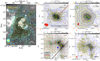 |
Fig. 1. Multiscale view of the B field toward the massive star-forming region G31.41+0.31. Panel (a): B-field segments (yellow) observed with the JCMT POL-2 (this work) with a primary beam FWHM of 12.6″ (Mairs et al. 2021) plotted in steps of 1 pixel with a scale of 12″ overlaid on the Spitzer GLIMPSE 8 μm image and IRAM-30m N2H+ integrated-intensity map (cyan contours) from Beltrán et al. (2022b). Panel (b): B-field segments (yellow) observed with SMA plotted with a step of 1 pixel and JCMT POL-2 (red) overlaid on the Stokes I (blue and cyan contours) at 879 μm observed with the SMA and a synthesized beam of |


The plane-of-the-sky B-field strength (Bpos) estimated toward G31 at core scales is Bpos ∼ 10 mG (Girart et al. 2009; Beltrán et al. 2019). The values are as high as Bpos ∼ 50 mG toward the inner part of the HMC, where the four massive protostars are embedded (Beltrán et al. 2024).
To complete the multiscale study of the role of the B field in the G31 star-forming region, we carried out observations of the polarized dust emission with the James Clerk Maxwell Telescope (JCMT) POL-2 at 850 μm of the whole cloud. The first goal of the study was to compare and connect the B-field orientation that is observed at cloud scales with the orientation determined at circumstellar scales. We considered as cloud or large scales the scales at ≳30 000 au, as core scales the scales between ∼300 and ∼30 000 au, and as circumstellar or disk scales the scales ≲300 au. The second goal of the observations was to characterize the relative importance of the B field at the cloud scale by characterizing the B-field morphology and estimating the B-field strength via the Davis-Chandrasekhar-Fermi (DCF) method.
2. Observations and data reductions
We carried out single-field polarized dust observations at 850 μm using the Submillimetre Common-User Bolometer Array (SCUBA-2) plus POL-2 system toward the G31 star-forming region with the daisy-scan pattern. The observations were carried out as the individually funded program (project ID E21BJ001; P.I: R. Furuya) on 2021 July 17 and 18 under the JCMT Weather Band 1. The technical details and the data reduction pipelines we employed, such as the flux-conversion factor, the attenuation-correction factor due to the insertion of POL-2, the instrumental-polarization correction model, the debiasing method, and the definitions of the polarimetric quantities and their error calculations all were the same as those for the recent B-fields In STar-forming Region Observations (BISTRO-2 and BISTRO-3) surveys described by Arzoumanian et al. (2021), Wang et al. (2024a), and Choi et al. (2024). Because of the primary beam size at the 850 μm band (θHPBW ∼ 12 6; Mairs et al. 2021), we analyzed the Stokes I, Q, and U maps with a 12
 0 grid spacing. The estimated rms noise in Stokes I is ∼4 mJy beam−1, and for Stokes Q and U, it is 1.3 mJy beam−1. The B-field position angles were estimated from north to east.
3. Results
3.1. Multiscale view of the B field in the HMC
Figure 1 presents the overview of the dust continuum emission and the plane-of-sky B-field orientation (inferred by rotating the polarization angle by 90°) in G31 from cloud (panel a) to circumstellar scales (panel d). The position angles are defined starting from north, positive in the counterclockwise direction.
The B-field orientation at the cloud scale derived from the JCMT 850 μm dust polarization emission shows a clear dichotomy, in which the B field is preferentially aligned in the E–W direction toward the southern part of the cloud and in the NW–SE direction toward the northern part of the cloud (Fig. 1, panel a). This change in the B-field orientation appears to occur visually in the close vicinity of the HMC (orange square in panel a). To better quantify this and further characterize the variations in the cloud-scale B-field morphology, we carry out a detailed analysis in Sect. 3.2.
The B-field orientation obtained with the JCMT toward the position of the HMC is −45.2 ° ±19° (Fig. 1, panel a). This orientation is consistent with the NW–SE mean B-field direction observed at core scales with the Submillimeter Array (SMA) at a resolution of 879 μm and ∼4000 au (Fig. 1, panel b; Girart et al. 2009), with Atacama Large Millimeter Array (ALMA) at a spatial resolution of 1.3 mm and ∼900 au (Fig. 1, panel c; Beltrán et al. 2019), and at circumstellar scales with ALMA at a spatial resolution of 3.1 mm and ∼260 au (Fig. 1, panel d; Beltrán et al. 2024). Panel (e) summarizes all the B-field orientations observed at the different scales with the different telescopes and angular resolutions. The good visual agreement of the average B-field orientation is clear. Quantitatively, Girart et al. (2009) fit the magnetic field in the core with a position angle of ∼ − 27°, and Beltrán et al. (2019, 2024) modeled the B field at core and circumstellar scales with an axially symmetric singular toroid threaded by a poloidal B field (Li & Shu 1996; Padovani & Galli 2011). The best model obtained by the latter authors is consistent with an hourglass-shaped B field with a position angle of −44° at core scales and −63° at circumstellar scales. The cloud-scale B-field orientation coincides (within the errors) with the orientation measured at core and circumstellar scales. This good agreement in the orientation of the B field at all scales suggests that the B field might be connected from cloud to circumstellar scales, despite the difference of some orders of magnitude in density and spatial scales. We carried out a quantitative multiscale comparison of the JCMT B-field orientation at the center of intensity (CI)1. The position of the CI is RA(J2000):  32 and Dec (J2000):
−01°12 , with the B-field orientation obtained from the different SMA and ALMA images at wavelengths of 3.1 mm, 1.3 mm, and 879 μm centered on the four continuum protostars embedded in the HMC, named A to D by Beltrán et al. (2021), and on the source NE, located northeast of the HMC (Beltrán et al. 2021). In practice, we obtained the simple angular mean and standard deviation of the B-field angles over different spatial apertures ranging from the highest angular resolution of ALMA (∼0
 or ∼260 au) to that of the SMA (∼1
 or ∼5000 au). At each wavelength, the spatial aperture was increased from the smallest aperture size defined by the diameter equivalent to the major axis of the synthesized beam of each interferometer up to ten times the original aperture diameter with a step size equal to the major axis of the corresponding beam size. Figure 2 shows the angle difference (Δθ) between the JCMT values and the averaged values obtained with the different apertures. The corresponding errors in Δθ were propagated from the standard deviation of the B-field orientation in the aperture and the uncertainty in the B-field orientation. At the CI position, we found that the B-field orientation remained similar at all scales (from 260 au up to 5 × 10³ au) with deviations not greater than 20 ° ±19°. This confirms that the orientation of the hourglass-shaped B field remains similar down to the circumstellar scale. The low Δθ across different scales also suggests that feedback or turbulence does not severely affect the collapsing core. At the position of the protostars, all of them maintain coherence down to ∼104 au. Below 104 au, the B field around source D first starts to deviate significantly. The same occurs for source C, and to lesser extent, for source B, at scales smaller than ∼3000 au. In contrast, source A (which lies closer to the CI) maintains a coherent field with Δθ ∼ 20°. In other words, the farther the massive protostar from the CI, the stronger the deviation in the orientation of the associated circumstellar B field from the orientation of the large-scale B-field. This does not occur for source NE, which is a different core and is not associated with the protocluster. The B-field orientation toward the NE source remains coherent down to 1000 au.
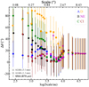 |
Fig. 2. Angle difference (Δθ) and errors in Δθ between the cloud-scale B-field orientation and the mean B-field orientation toward the four embedded protostars (A-D), their center of intensity (CI), and the continuum source NE identified in Beltrán et al. (2021). The spatial scale is increased from the smallest aperture size defined by the diameter equivalent to the major axis of the synthesized beam of each interferometer up to ten times the original aperture diameter. Each symbol represents data obtained from different telescopes. Circle: ALMA 3.1 mm data with a synthesized beam of |


We interpret the correlation between the distances of sources A–D to the CI position and Δθ as follows. For a collapsing core threaded with an initially uniform ambient B field, the contraction of the infalling medium will drag and distort the B field toward the mass center of the core, resulting in an hourglass morphology of the B field (Galli & Shu 1993; Basu & Mouschovias 1994). The B field toward the protostar(s) that dominates the infall in the core (i.e., closer to the CI position) is expected to be more strongly influenced by the collapse, and therefore, the circumstellar B field is expected to have a more prominently hourglass-shaped morphology. This is in fact the case in G31. The B-field orientation measured by the JCMT is a mass-weighted average of the B-field direction inside a large area with a size of ∼0.2 pc, which corresponds to its beam. Similarly, the B-field morphology toward sources A and B, located at the center of the core, resembles an hourglass with approximately the same orientation as on cloud scales, although we cannot distinguish whether it is a single hourglass or one around each source based on the current data (see Fig. 1, panel d). These sources exhibit the strongest redshifted absorption (i.e., inverse P-Cygni) profile in high-density tracers such as CH3CN, which was interpreted as infall by Beltrán et al. (2022b). Source A, which is the source located closest to the CI position, has the most prominent inverse P-Cygni profile and also shows the lowest Δθ from cloud to circumstellar scales. In this scenario, the infall onto these sources would dominate the global collapse of the core, drag the B field, and preserve a self-similar orientation at all scales. The redshifted absorption profiles are less evident toward sources C and D (Beltrán et al. 2022b), which are located farther from the CI position. This suggests that the infall of the core could affect the circumstellar B field less. As a result, the circumstellar B-field orientation of sources C and D could differ significantly from the orientation at core and cloud scales.
Figure A.1 presents the JCMT POL-2 Stokes I contours overlaid on the polarized intensity, pI, and polarized fraction, p, maps of the G31 hub-filament system. The dust emission at 850 μm peaks toward the HMC position, and the overall cloud morphology is similar to that traced by N2H+ (Fig. 1, panel a). Turning to pI, it peaks at the position of the HMC (pI = 55 mJy beam−1). We also note a secondary local maximum, which corresponds to the less evolved southern core identified by Beltrán et al. (2022a). The p map shows a polarization hole (p < 2%) toward the Stokes I peak. This likely is the result of the large JCMT beam that smears the complex small-scale B-field morphology (e.g., Wang et al. 2024b).
3.2. Polarized emission and B-field properties of the G31 hub-filament system
We estimated the total (ordered plus turbulent) plane-of-sky B-field strength ( ) of the G31 hub-filament system using the JCMT data by applying the Davis-Chandrasekhar-Fermi (DCF) method (Davis 1951; Chandrasekhar & Fermi 1953; Ostriker et al. 2001) and a variation of the DCF method (ST-DCF; Skalidis & Tassis 2021) using a number density nH of (6.9 ± 0.5)×103 cm−3 estimated from the N2H+ observations carried out with the IRAM-30m by Beltrán et al. (2022a, see our Appendix B for the detailed calculations). We assumed that the cloud morphology can be described with a cylindrical geometry. The estimated
  is 0.04 ± 0.004 mG using the DCF method and
  mG using the ST-DCF variation. Although these estimates of the B-field strength have to be taken with caution in light of the uncertainties of these statistical methods and of the uncertainties in N2H+ abundance, cloud geometry, and line-of-sight depth, they are consistent with the strenghts obtained with similar densities and methods (Bpos, DCF ∼ 0.02–0.5 mG, see Pattle et al. 2023, and references therein). We also evaluated the relative importance of the B field compared to gravity and turbulence via the ratio of mass to magnetic flux (λ) and the ratio of turbulent to magnetic energy (βturb; see Appendix B for the detailed calculations). The estimated λ is 6 ± 0.8 for DCF and 3 ± 0.3 for ST-DCF. The resulting λ ≫ 1 suggests a strongly supercritical state in which gravity dominates the B field. The calculated βturb = 6.9 ± 1.6 for DCF and 1.2 ± 0.4 for ST-DCF suggests that the B field might be less important than turbulence in the energy budget of the G31 hub-filament system, although βturb is very sensitive to the value of the B-field strength as it is ∝1/B2.
A clear feature of the G31 hub-filament B-field morphology in Fig. 1 (panel a) is that the large-scale B-field orientation in the G31 hub-filament system shows a bimodal distribution as it changes from an E–W direction in the southern part to an NW–SE direction in the northern part of the hub-filament. To better quantify this change, we plot in Fig. 3 the average of the B-field orientation in the direction of the right ascension (|〈θB〉|RA) as a function of the declination (θdec) offset from the HMC declination position. This figure shows a change in (|θB|RA) as a function of declination. For negative offsets, which correspond to the southern part of the cloud, the orientation is between 60°–90°, while for positive offsets, which correspond to the northern part, the orientation is between 30°–60°. Moreover, the dispersion in |〈θB〉|RA is higher to the north than to the south. We note that the change in |〈θB〉|RA occurs toward the declination of the HMC.
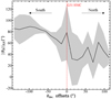 |
Fig. 3. Profile of the mean B-field orientation in the direction of the right ascension (|〈θB〉|RA) as a function of angular offsets along the direction of the declination (θdec) from the HMC position. The dotted red line represents the location of the HMC. Each average B-field orientation was computed by taking the angle average in the RA direction at each declination position. The shaded region represents the dispersion of the B-field orientation. |
The clear change in the mean B-field orientation and the fact that the transition occurs at the position of the HMC might provide some insights into the formation scenario of the G31 star-forming region. One possibility is that the hub-filament system was formed via a cloud-cloud collision that triggered star formation in the HMC, as suggested by Beltrán et al. (2022a) in the context of the paradigm of filaments to clusters (see Kumar et al. 2020, for a detailed description of this paradigm). In this case, the different B-field orientation to the north and south of the hub-filament system would be the remnant of the original B-field orientation of the two colliding clouds before the collision. The cloud-cloud collision scenario in G31 is further supported by the fact that the N2H+ spectra show a double velocity component at the position of the HMC and also by the line velocity (moment 1) map of the N2H+ satellite line, which clearly shows different velocities for the northern and southern part of the cloud (see Figs. 1 and 2 of Beltrán et al. 2022a). A similar scenario was proposed for the bowl region of the Pipe nebula by Frau et al. (2015). By comparing the data with magnetohydrodynamics simulations, these authors showed that the B field and gas kinematical properties in the Pipe nebula can also be explained by a cloud-cloud collision. Arzoumanian et al. (2021) also proposed a cloud-cloud collision to explain the change in the B-field orientation along the filament in NGC 6334. If this scenario were confirmed, the B-field strength would need to be calculated separately for each cloud.
An alternative scenario to explain the different B-field properties in the northern and southern parts of the G31 hub-filament system would be a different B-field complexity in the two regions. In the northern part, which is associated with an active site of massive star formation that contains the HMC and a nearby ultracompact H II region, the B field would be more disturbed by turbulence and gravity associated with the star-forming process itself. This would result in a higher dispersion of the B-field orientation and a lower polarization fraction, as observed in Figs. 3 and A.1, respectively. In contrast, the southern part of the system would be in a more quiescent phase with no signs of star formation activity that could perturb and significantly alter the B-field properties, in particular, its orientation. Although we cannot discard either scenario as both are consistent with the available data, we favor the cloud-cloud collision scenario based on the N2H+ analysis of Beltrán et al. (2022a) and the very different B-field orientation and properties in the different parts of the cloud.
4. Conclusions
We presented a multiscale study of the B-field properties of the HMC, which is embedded in a hub-filament system. This study revealed that the orientation of the hourglass B field observed at core and circumstellar scales with ALMA and SMA observations of polarized dust emission is preserved at the large cloud scales that are traced by the JCMT POL-2 observations. This self-similarity in the B-field orientation suggests that the field is connected from cloud to circumstellar scales despite the difference in density and spatial scales. In this sense, the B field from circumstellar to cloud scales might be dominated by the formation of the more intense protostars that are embedded in the HMC (sources A and B), which clearly show an hourglass-shaped B field at the highest angular resolution and the deepest redshifted absorption.
The orientation of the B field in the G31 hub-filament system shows a bimodal distribution, in which the B field is preferentially aligned in the E–W direction to the southern part and in the NW–SE direction in the northern part of the cloud. The change in the orientation appears to occur in the close vicinity of the G31 HMC. Together with the fact that the polarized intensity and polarized fraction are slightly different north and south of the hub-filament system, this bimodality favors the scenario of a cloud-cloud collision for the formation of this star-forming region. In this scenario, the different properties of the B field observed north and south of the cloud would be the remnant of those originally present before the collision. Finally, we found that the B-field strength on the plane of the sky in the cloud as estimated with the DCF method ranges from 0.04 to 0.09 mG.
We defined the CI as the mean position of the four protocluster sources in G31, A-D, weighted by their corresponding peak intensity at 3.1 mm (indicated with a blue cross in Fig. 1, panel e).
Acknowledgments
C-Y.L., M.T.B., D.G., L.M., R.C., M.P., A.S, G.S. acknowledge financial support through the INAF Large Grant The role of MAGnetic fields in MAssive star formation (MAGMA). This work is supported in part by a Grant-in-Aid for Scientific Research of Japan (19H01938 and 21H00033). RSF was supported by the Visiting Scholars Program provided by the NAOJ Research Coordination Committee, NINS (NAOJ-RCC-23DS-050). J.M.G. acknowledges support by the grant PID2023-146675NB-I00 (MCIU-AEI-FEDER, UE). This work is also partially supported by the program Unidad de Excelencia María de Maeztu CEX2020-001058-M.
References
- Arzoumanian, D., Furuya, R. S., Hasegawa, T., et al. 2021, A&A, 647, A78 [NASA ADS] [CrossRef] [EDP Sciences] [Google Scholar]
- Basu, S., & Mouschovias, T. C. 1994, ApJ, 432, 720 [NASA ADS] [CrossRef] [Google Scholar]
- Beltrán, M. T., Cesaroni, R., Neri, R., et al. 2005, A&A, 435, 901 [Google Scholar]
- Beltrán, M. T., Codella, C., Viti, S., Neri, R., & Cesaroni, R. 2009, ApJ, 690, L93 [Google Scholar]
- Beltrán, M. T., Cesaroni, R., Rivilla, V. M., et al. 2018, A&A, 615, A141 [Google Scholar]
- Beltrán, M. T., Padovani, M., Girart, J. M., et al. 2019, A&A, 630, A54 [Google Scholar]
- Beltrán, M. T., Rivilla, V. M., Cesaroni, R., et al. 2021, A&A, 648, A100 [Google Scholar]
- Beltrán, M. T., Rivilla, V. M., Kumar, M. S. N., Cesaroni, R., & Galli, D. 2022a, A&A, 660, L4 [NASA ADS] [CrossRef] [EDP Sciences] [Google Scholar]
- Beltrán, M. T., Rivilla, V. M., Cesaroni, R., et al. 2022b, A&A, 659, A81 [NASA ADS] [CrossRef] [EDP Sciences] [Google Scholar]
- Beltrán, M. T., Padovani, M., Galli, D., et al. 2024, A&A, 686, A281 [NASA ADS] [CrossRef] [EDP Sciences] [Google Scholar]
- Carey, S. J., Noriega-Crespo, A., Mizuno, D. R., et al. 2009, PASP, 121, 76 [Google Scholar]
- Cesaroni, R., Churchwell, E., Hofner, P., Walmsley, C. M., & Kurtz, S. 1994, A&A, 288, 903 [NASA ADS] [Google Scholar]
- Chandrasekhar, S., & Fermi, E. 1953, ApJ, 118, 113 [Google Scholar]
- Choi, Y., Kwon, W., Pattle, K., et al. 2024, ApJ, 977, 32 [Google Scholar]
- Colzi, L., Rivilla, V. M., Beltrán, M. T., et al. 2021, A&A, 653, A129 [NASA ADS] [CrossRef] [EDP Sciences] [Google Scholar]
- Davis, L. 1951, Phys. Rev., 81, 890 [Google Scholar]
- Fontani, F., Mininni, C., Beltrán, M. T., et al. 2024, A&A, 682, A74 [NASA ADS] [CrossRef] [EDP Sciences] [Google Scholar]
- Frau, P., Girart, J. M., Alves, F. O., et al. 2015, A&A, 574, L6 [NASA ADS] [CrossRef] [EDP Sciences] [Google Scholar]
- Galli, D., & Shu, F. H. 1993, ApJ, 417, 220 [NASA ADS] [CrossRef] [Google Scholar]
- Girart, J. M., Beltrán, M. T., Zhang, Q., Rao, R., & Estalella, R. 2009, Science, 324, 1408 [NASA ADS] [CrossRef] [Google Scholar]
- Hacar, A., Tafalla, M., & Alves, J. 2017, A&A, 606, A123 [NASA ADS] [CrossRef] [EDP Sciences] [Google Scholar]
- Houde, M., Vaillancourt, J. E., Hildebrand, R. H., Chitsazzadeh, S., & Kirby, L. 2009, ApJ, 706, 1504 [Google Scholar]
- Houde, M., Fletcher, A., Beck, R., et al. 2013, ApJ, 766, 49 [Google Scholar]
- Houde, M., Hull, C. L. H., Plambeck, R. L., Vaillancourt, J. E., & Hildebrand, R. H. 2016, ApJ, 820, 38 [NASA ADS] [CrossRef] [Google Scholar]
- Hull, C. L. H., Girart, J. M., Tychoniec, Ł., et al. 2017, ApJ, 847, 92 [NASA ADS] [CrossRef] [Google Scholar]
- Immer, K., Li, J., Quiroga-Nuñez, L. H., et al. 2019, A&A, 632, A123 [NASA ADS] [CrossRef] [EDP Sciences] [Google Scholar]
- Kauffmann, J., Bertoldi, F., Bourke, T. L., Evans, N. J., II, & Lee, C. W. 2008, A&A, 487, 993 [NASA ADS] [CrossRef] [EDP Sciences] [Google Scholar]
- Koch, P. M., Tang, Y.-W., Ho, P. T. P., et al. 2022, ApJ, 940, 89 [NASA ADS] [CrossRef] [Google Scholar]
- Kumar, M. S. N., Palmeirim, P., Arzoumanian, D., & Inutsuka, S. I. 2020, A&A, 642, A87 [EDP Sciences] [Google Scholar]
- Law, C.-Y., Tan, J. C., Skalidis, R., et al. 2024, ApJ, 967, 157 [Google Scholar]
- Li, Z.-Y., & Shu, F. H. 1996, ApJ, 472, 211 [NASA ADS] [CrossRef] [Google Scholar]
- Li, H. B., Goodman, A., Sridharan, T. K., et al. 2014, in Protostars and Planets VI, eds. H. Beuther, R. S. Klessen, C. P. Dullemond, & T. Henning, 101 [Google Scholar]
- Li, H.-B., Yuen, K. H., Otto, F., et al. 2015, Nature, 520, 518 [Google Scholar]
- Liu, J., Qiu, K., & Zhang, Q. 2022a, ApJ, 925, 30 [NASA ADS] [CrossRef] [Google Scholar]
- Liu, J., Zhang, Q., & Qiu, K. 2022b, Front. Astron. Space Sci., 9, 943556 [NASA ADS] [CrossRef] [Google Scholar]
- Liu, J., Zhang, Q., Koch, P. M., et al. 2023, ApJ, 945, 160 [NASA ADS] [CrossRef] [Google Scholar]
- Liu, J., Zhang, Q., Lin, Y., et al. 2024, ApJ, 966, 120 [Google Scholar]
- Machida, M. N., Inutsuka, S.-i., & Matsumoto, T. 2007, ApJ, 670, 1198 [NASA ADS] [CrossRef] [Google Scholar]
- Mairs, S., Dempsey, J. T., Bell, G. S., et al. 2021, AJ, 162, 191 [NASA ADS] [CrossRef] [Google Scholar]
- Maury, A., Hennebelle, P., & Girart, J. M. 2022, Front. Astron. Space Sci., 9, 949223 [NASA ADS] [CrossRef] [Google Scholar]
- Mininni, C., Beltrán, M. T., Rivilla, V. M., et al. 2020, A&A, 644, A84 [NASA ADS] [CrossRef] [EDP Sciences] [Google Scholar]
- Osorio, M., Anglada, G., Lizano, S., & D’Alessio, P. 2009, ApJ, 694, 29 [Google Scholar]
- Ostriker, E. C., Stone, J. M., & Gammie, C. F. 2001, ApJ, 546, 980 [Google Scholar]
- Padovani, M., & Galli, D. 2011, A&A, 530, A109 [NASA ADS] [CrossRef] [EDP Sciences] [Google Scholar]
- Pattle, K., Fissel, L., Tahani, M., Liu, T., & Ntormousi, E. 2023, in Protostars and Planets VII, eds. S. Inutsuka, Y. Aikawa, T. Muto, K. Tomida, & M. Tamura, ASP Conf. Ser., 534, 193 [Google Scholar]
- Rivilla, V. M., Beltrán, M. T., Cesaroni, R., et al. 2017, A&A, 598, A59 [NASA ADS] [CrossRef] [EDP Sciences] [Google Scholar]
- Skalidis, R., & Tassis, K. 2021, A&A, 647, A186 [NASA ADS] [CrossRef] [EDP Sciences] [Google Scholar]
- Skalidis, R., Sternberg, J., Beattie, J. R., Pavlidou, V., & Tassis, K. 2021, A&A, 656, A118 [NASA ADS] [CrossRef] [EDP Sciences] [Google Scholar]
- Tan, J. C., Beltrán, M. T., Caselli, P., et al. 2014, in Protostars and Planets VI, eds. H. Beuther, R. S. Klessen, C. P. Dullemond, & T. Henning, 149 [Google Scholar]
- Wang, J.-W., Koch, P. M., Clarke, S. D., et al. 2024a, ApJ, 962, 136 [Google Scholar]
- Wang, L., Cao, Z., Fan, X., & Li, H.-B. 2024b, ApJ, 966, 237 [Google Scholar]
Appendix A: Polarized fraction and polarized intensity map of G31 hub-filament system
Figure A.1 presents the 850 μm JCMT POL-2 Stokes I map (contours) overlaid on the debiased polarized intensity pI (left panel) and the debiased polarized fraction p (right panel) map of the G31 hub-filament system. The debiasing method, the definitions of the polarimetric metrics, and their error calculations have been performed following the prescriptions described in the BISTRO-2 and BISTRO-3 survey papers (e.g., Wang et al. 2024a; Choi et al. 2024; Arzoumanian et al. 2021).
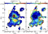 |
Fig. A.1. Left: JCMT POL-2 850 μm Stokes I intensity contours overlaid on the debiased polarized fraction, p. The contours levels are [10, 20, 40, 60, 80, 100, 200, 400]× σ, where σ = 4 mJy beam−1. Right: Same as the left panel, with the colormap now showing the debiased polarized intensity, pI. The yellow box in the two panels indicate the region used for B-field strength estimates (see Appendix B for details). The JCMT beam is shown in the bottom left corner of each panel. |
Appendix B: DCF B-field strength estimates
We have estimated the plane-of-the-sky B-field strength Bpos of the G31 hub-filament system with the DCF method. The DCF method assumes that the gas is perfectly attached to the B-field lines, the B-field line perturbations propagate in the form of small-amplitude incompressible magneto-hydrodynamic waves, and turbulent and magnetic energies are in equipartition. Following the notation of Eq. (26) in Houde et al. (2016), the DCF method estimates the strength via
 (B.1)
(B.1)
where Q is a a correction factor derived from turbulent cloud simulations (e.g., Ostriker et al. 2001), ρ is the gas density, σv is the 1-D velocity dispersion, and Bturb/B(turb + ord) is the ratio between the turbulent and total (ordered+turbulent) B-field components. The corresponding uncertainties in  is computed via error propagation
There are different methods to estimate the Bturb/B(turb + ord) ratio but it is usually calculated via the dispersion of polarization position angles (e.g., see review by Liu et al. 2022b). In this work, we estimated the Bturb/B(turb + ord) ratio via the calibrated angular dispersion function (ADF; Houde et al. 2009, 2016)
The Bturb/B(turb + ord) ratio can be evaluated from the ADF in the form of Eq. (22) in Houde et al. (2013)
![Mathematical equation: $$ \begin{aligned} 1-\langle \cos [\Delta \Phi (l)]\rangle \simeq \frac{\left\langle B_{\rm turb}{ }^2\right\rangle }{\left\langle B_{(\mathrm turb+ord)}^2\right\rangle } \times \left[\frac{\sqrt{2\pi }\delta ^3}{\left(\delta ^2+2 W^2\right) \Delta ^{\prime }}\right]\\ \times \left(1-e^{-l^2 / 2\left(\delta ^2+2 W^2\right)}\right) +a_2^{\prime } l^2, \end{aligned} $$](/articles/aa/full_html/2025/05/aa53510-24/aa53510-24-eq18.gif)
where ΔΦ(l) is the angular difference of two B-field position angles separated by a distance l, δ is the turbulent correlation length, assumed to be smaller than the cloud size, Δ′ is the effective line-of-sight depth of the cloud, W is the beam standard deviation (i.e., beam FWHM divided by  ), and a2′l2 is the first term of the Taylor expansion of the ordered component of ADF.
A modified version of the DCF method proposed by Skalidis & Tassis (2021, ST-DCF) relaxes the incompressibility assumption of DCF. Despite some doubts on the validity (e.g., Liu et al. 2022b), the ST-DCF is expected to be more accurate in regions of sub- to trans-Alfvénic turbulence, where it results in lower B-field strengths than those estimated with the DCF method (Skalidis et al. 2021). The corresponding B-field strength computed via the ST-DCF method is expressed as
 (B.2)
(B.2)
and the corresponding uncertainties in  is
is
To estimate Bpos, we consider that the cloud can be approximated as a cylinder elongated in the declination direction and with its rotation axis in the N–S direction, and construct the corresponding ADF over the region of the G31 hub-filament system defined by the yellow box in Fig. A.1, which has a dimension of 0.045 ° ×0.060°. Although some extended structures were not included in the analysis, these structures only contribute to relatively smaller areas of the hub-filament system and had a minor impact on the results of the ADF analysis. To construct the ADF, we also assume that the average line-of-sight depth of the cloud is approximated to be the radius (R) of the cylinder. We argue that varying the LOS depth from 0.5R to 2R does not impact the energetics estimates and the conclusions in this work. Hence, we adopt a line-of-sight depth of the cloud equivalent to R. We present the corresponding ADF adopting a bin step of half a beam size (6″) in Fig. B.1. We fitted the ADF by minimizing χ2 and obtained the best fits for Bturb/B(turb+ord) = 0.5 ± 0.04.
We also obtained σv and ρ as follows. The averaged σv was evaluated by fitting with MADCUBA the averaged N2H+ spectrum of the cloud (see Fig. B.2) using the observations carried out with the IRAM-30m by Beltrán et al. (2022a), and we obtained a similar average σv = 1.5 ± 0.03 km s−1.
Following Beltrán et al. (2022a), we assumed an N2H+ abundance of ∼2.5 × 10⁻¹⁰ (Hacar et al. 2017) and a mean molecular weight of molecular hydrogen of μ = 2.8 (Kauffmann et al. 2008). The total mass M is calculated via the following equation
 (B.3)
(B.3)
The N2H+ column density obtained with MADCUBA is N(N2H+) = (1.2 ± 0.3)×1013cm−2, and the estimated total mass is M = (1.3 ± 0.1)×104 M⊙. The corresponding number (nH) density and ρ are (6.9 ± 0.5)×103 cm−3 and (3.2 ± 0.2)×10−20 g cm−3, respectively.
With the correction factor Q of 0.21 (Eq. 7 of Liu et al. 2022a), we obtained  mG. Applying the same values of σv, ρ, and
  as above, we obtained
  mG.
mG.
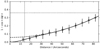 |
Fig. B.1. ADF of G31 hub-filament system defined by the rectangular region defined in Fig. A.1. Open circles represent the observed data, with the error bars indicating the dispersion. The best fit is shown by a solid line, and the dashed line represents the ordered component (a2′l2) of the best fit. The dotted vertical line and the horizontal lines, respectively, represent the beam size (12.6″) and the expected value for random B field ((1−cos〈Δϕ〉 = 0.36, Liu et al. 2022b). |
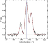 |
Fig. B.2. N2H+ average spectrum (black line) obtained by averaging the emission over the rectangular region illustrated in Fig. A.1 and corresponding fit computed with MADCUBA (red line). The dashed blue line represents the fitted systemic velocity (96.6 km s−1) of the region. |
Appendix C: Energy balance
Using the values of Bpos in the previous section, we calculated the mass-to-magnetic flux ratio normalized to the critical value, λ, in the form
 (C.1)
(C.1)
where G is the gravitational constant, M is the mass of the region defined in Eq. (B.4) and Φ = Btot × Area is the magnetic flux, where Btot is the total B-field strength estimated as  , with i being the inclination with respect to the plane of the sky. Taking this into account, λ can be expressed as
 (C.2)
(C.2)
Assuming that the inclination of the B field at cloud scales is the same as that estimated at core scales by Beltrán et al. (2024), that is i = 50°, then λ = 6 ± 0.8 and 3 ± 0.3 respectively for DCF and ST-DCF.
We also computed the turbulent-to-magnetic energy ratio βturb, following Law et al. (2024), as
 (C.3)
(C.3)
where  is the Alfvén speed, which is equal to 1 ± 0.11 km s−1 for DCF and 2.3 ± 0.17 km s−1 for ST-DCF.
The estimated βturb is 6.9 ± 1.6 for DCF and 1.2 ± 0.4 for ST-DCF.
All Figures
|
Fig. 1. Multiscale view of the B field toward the massive star-forming region G31.41+0.31. Panel (a): B-field segments (yellow) observed with the JCMT POL-2 (this work) with a primary beam FWHM of 12.6″ (Mairs et al. 2021) plotted in steps of 1 pixel with a scale of 12″ overlaid on the Spitzer GLIMPSE 8 μm image and IRAM-30m N2H+ integrated-intensity map (cyan contours) from Beltrán et al. (2022b). Panel (b): B-field segments (yellow) observed with SMA plotted with a step of 1 pixel and JCMT POL-2 (red) overlaid on the Stokes I (blue and cyan contours) at 879 μm observed with the SMA and a synthesized beam of |
| In the text | |
|
Fig. 2. Angle difference (Δθ) and errors in Δθ between the cloud-scale B-field orientation and the mean B-field orientation toward the four embedded protostars (A-D), their center of intensity (CI), and the continuum source NE identified in Beltrán et al. (2021). The spatial scale is increased from the smallest aperture size defined by the diameter equivalent to the major axis of the synthesized beam of each interferometer up to ten times the original aperture diameter. Each symbol represents data obtained from different telescopes. Circle: ALMA 3.1 mm data with a synthesized beam of |
| In the text | |
|
Fig. 3. Profile of the mean B-field orientation in the direction of the right ascension (|〈θB〉|RA) as a function of angular offsets along the direction of the declination (θdec) from the HMC position. The dotted red line represents the location of the HMC. Each average B-field orientation was computed by taking the angle average in the RA direction at each declination position. The shaded region represents the dispersion of the B-field orientation. |
| In the text | |
|
Fig. A.1. Left: JCMT POL-2 850 μm Stokes I intensity contours overlaid on the debiased polarized fraction, p. The contours levels are [10, 20, 40, 60, 80, 100, 200, 400]× σ, where σ = 4 mJy beam−1. Right: Same as the left panel, with the colormap now showing the debiased polarized intensity, pI. The yellow box in the two panels indicate the region used for B-field strength estimates (see Appendix B for details). The JCMT beam is shown in the bottom left corner of each panel. |
| In the text | |
|
Fig. B.1. ADF of G31 hub-filament system defined by the rectangular region defined in Fig. A.1. Open circles represent the observed data, with the error bars indicating the dispersion. The best fit is shown by a solid line, and the dashed line represents the ordered component (a2′l2) of the best fit. The dotted vertical line and the horizontal lines, respectively, represent the beam size (12.6″) and the expected value for random B field ((1−cos〈Δϕ〉 = 0.36, Liu et al. 2022b). |
| In the text | |
|
Fig. B.2. N2H+ average spectrum (black line) obtained by averaging the emission over the rectangular region illustrated in Fig. A.1 and corresponding fit computed with MADCUBA (red line). The dashed blue line represents the fitted systemic velocity (96.6 km s−1) of the region. |
| In the text | |
Current usage metrics show cumulative count of Article Views (full-text article views including HTML views, PDF and ePub downloads, according to the available data) and Abstracts Views on Vision4Press platform.
Data correspond to usage on the plateform after 2015. The current usage metrics is available 48-96 hours after online publication and is updated daily on week days.
Initial download of the metrics may take a while.