| Issue |
A&A
Volume 699, July 2025
|
|
|---|---|---|
| Article Number | A14 | |
| Number of page(s) | 13 | |
| Section | Extragalactic astronomy | |
| DOI | https://doi.org/10.1051/0004-6361/202452697 | |
| Published online | 30 June 2025 | |
NEUTRALUNIVERSEMACHINE: Predictions of H I gas in different theoretical models
1
Shanghai Astronomical Observatory, Chinese Academy of Sciences, Shanghai 200030, China
2
University of Chinese Academy of Sciences, Beijing 100049, China
3
Tianjin Normal University, Binshuixidao 393, 300387 Tianjin, China
4
INAF-Astronomical Observatory of Trieste, Via G.B. Tiepolo, 11 I-34143 Trieste, Italy
5
IFPU – Institute for Fundamental Physics of the Universe, via Beirut 2, I-34151 Trieste, Italy
6
DARK, Niels Bohr Institute, University of Copenhagen, Lyngbyvej 2, DK-2100 Copenhagen, Denmark
⋆ Corresponding author: guohong@shao.ac.cn
Received:
22
October
2024
Accepted:
23
May
2025
We investigate the distribution and evolution of H I gas in different theoretical models, including hydrodynamical simulations of IllustrisTNG and SIMBA, the semi-analytical model of GAEA, and the empirical model of NEUTRALUNIVERSEMACHINE (NUM). By comparing model predictions for the H I mass function (HIMF), H I-halo and H I-stellar mass relations, conditional H I mass function (CHIMF) and the halo occupation distribution (HOD) of H I-selected galaxies, we find that all models show reasonable agreement with the observed HIMF at z ∼ 0. However, the differences become much larger at higher redshifts of z = 1 and z = 2. The HIMF of NUM shows remarkable agreement with the observation at z = 1, whereas other models predict much smaller amplitudes of HIMF at the high-mass end. Comparisons of CHIMF distributions indicate that the HIMF is dominated by haloes of 10 < log(Mvir/M⊙) < 11 and 11 < log(Mvir/M⊙) < 12 at the low- and high-mass ends, respectively. From the H I HODs of central galaxies, we find that TNG100 overpredicts the number of central galaxies with high MH I in massive haloes, and that GAEA shows a very strong depletion of H I gas in quenched centrals of massive haloes. The main cause of these differences is the AGN feedback mechanisms implemented in different models.
Key words: galaxies: halos / intergalactic medium / galaxies: star formation
© The Authors 2025
 Open Access article, published by EDP Sciences, under the terms of the Creative Commons Attribution License (https://creativecommons.org/licenses/by/4.0), which permits unrestricted use, distribution, and reproduction in any medium, provided the original work is properly cited.
This article is published in open access under the Subscribe to Open model. Subscribe to A&A to support open access publication.
1. Introduction
Cold gas, composed mainly of atomic and molecular elements, with atomic hydrogen (H I) playing a major role, acts as the essential fuel for star formation. Consequently, investigating the H I distribution is vital for understanding the processes of galaxy formation and its interaction with dark matter haloes, and it can also facilitate comprehension of the large-scale structure of galaxies. The distribution of the H I gas in the Local Universe has been accurately mapped through H I 21 cm surveys, such as the H I Parkes All-Sky Survey (HIPASS; Barnes et al. 2001; Meyer et al. 2004), the Arecibo Fast Legacy ALFA Survey (ALFALFA; Giovanelli et al. 2005; Haynes et al. 2011), the HI Nearby Galaxy Survey (THINGS; Walter et al. 2008), the GALEX Arecibo SDSS Survey (GASS Catinella et al. 2010), the Apertif survey (Adams et al. 2022) and the FAST All Sky H I Survey (FASHI; Zhang et al. 2024). However, detecting individual galaxies becomes increasingly challenging at higher redshifts because of weak signals and radio frequency interference. To overcome this, techniques such as H I spectra stacking and intensity mapping have been used to estimate the cosmic H I density for redshifts up to z < 1 (e.g. Lah et al. 2007; Delhaize et al. 2013; Masui et al. 2013; Rhee et al. 2013, 2018, 2023; Kanekar et al. 2016; Bera et al. 2019; Guo et al. 2020; Dev et al. 2023). At even higher redshifts (z > 1.5), the cosmic H I density can be measured using damped Lyα systems (DLAs; Wolfe et al. 2005), which are detected through absorption lines in the spectra of background quasars (e.g. Péroux et al. 2003; Prochaska et al. 2005; Prochaska & Wolfe 2009; Noterdaeme et al. 2009, 2012; Crighton et al. 2015; Neeleman et al. 2016; Bird et al. 2016).
However, simulations can provide an opportunity to understand the underlying physical processes. Various models have been proposed to explain the observations, including hydrodynamical simulations, semi-analytical models (SAMs), and empirical models. Depending on the adopted subgrid physics in modelling the galaxy formation and evolution, hydrodynamical simulations can reasonably replicate the observations in the stellar components, such as the stellar mass function and star formation rate. However, the H I and H2 gas properties in these simulations could vary significantly. As shown in Davé et al. (2020), the hydrodynamical simulations of SIMBA (Davé et al. 2019), IllustrisTNG (Nelson et al. 2019), and EAGLE (Schaye et al. 2014; Crain et al. 2015) exhibit strong differences in their H I properties, particularly at higher redshifts.
One of the key challenges in hydrodynamical simulations is the extensive resource requirement needed to conduct large-volume, high-resolution simulations. Modelling the atomic-to-molecular hydrogen transition from first principles is extremely challenging. Therefore, it is generally treated using a post-processing framework (Duffy et al. 2012; Lagos et al. 2015; Diemer et al. 2018), similar to the approach used in SAMs (see e.g. Fu et al. 2010, 2013; Lagos et al. 2011; Xie et al. 2017). By leveraging halo merger trees from high-resolution N-body simulations, SAMs can effectively model the cold-gas components of galaxies over significantly larger volumes compared to hydrodynamical simulations. However, the varied approaches of galaxy formation employed in these models can result in notable differences in statistics that are typically uncalibrated. For example, Baugh et al. (2019) identified substantial variations in the H I -halo mass relations between different models, especially for haloes with Mvir > 1011.5 M⊙ where the AGN feedback becomes a significant factor (see also Chauhan et al. 2020; Spinelli et al. 2020). A recent study of Hutchens et al. (2025) also found that AGN-hosting haloes exhibit significantly lower H I-halo mass ratios compared to non-AGN haloes, confirming the importance of carefully modelling the effect of AGN feedback.
In practice, although the parameter space is large, it is difficult for SAMs to fit all the available stellar and cold-gas observational measurements well (see e.g. Henriques et al. 2015). Using simple functional forms without involving detailed baryon physics, empirical models become another popular way to statistically link the properties of galaxies and their halo environment (see e.g. Behroozi et al. 2013, 2019; Popping et al. 2015). Recently, Guo et al. (2023) proposed a new empirical model, NEUTRALUNIVERSEMACHINE (hereafter NUM), which can accurately reproduce the observed cold gas properties. Their model parameters are calibrated by fitting to the available H I measurements, such as the H I mass function (HIMF) and H I-stellar mass relations. In addition to successfully fitting the observed H I scaling relations, it also provides useful predictions for the H I intensity mapping measurements (Li et al. 2024) and the H I-stellar mass relations at higher redshifts (Bianchetti et al. 2025).
However, empirical models such as NUM do not provide physical explanations for the functional forms of the H I relations. It is important to compare the model predictions of empirical models with hydrodynamical simulations and SAMs to understand the physical processes driving the observed scaling relations, similar to the common practice of comparing the galaxy stellar components (see e.g. Lagos et al. 2011; Popping et al. 2015; Baugh et al. 2019; Spinelli et al. 2020; Li et al. 2022). This is especially useful when comparing the scaling relations without robust H I measurements. In this study, we focus on model comparisons of H I properties in different halo environments. In particular, we explore the model predictions of the conditional H I mass function (CHIMF), and the halo occupation distribution (HOD) of H I-selected galaxies from z = 0 to z = 2, which are not calibrated with observations. Throughout the paper, we adopt the cosmology of Planck Collaboration XIII (2016) as in NUM. The influence of different cosmological parameters in various models is taken into account by correcting the halo mass definitions to be consistent with each other.
This paper is structured as follows. In Sect. 2, we introduce the simulations and data that we used. We present our main results in Sect. 3. In Sects. 4 and 5, we provide our discussions and conclusions.
2. Simulations
2.1. The IllustrisTNG simulation
The IllustrisTNG project consists of a set of magnetohydrodynamical simulations of different cosmological volumes (Marinacci et al. 2018; Naiman et al. 2018; Nelson et al. 2018, 2019; Pillepich et al. 2018; Springel et al. 2018), run with the Arepo code (Springel 2010). We focused only on the TNG100-1 simulation (referred to as TNG hereafter), which has a box size of 75 h−1Mpc on each side and the cosmological parameters of Ωm = 0.3089, Ωλ = 0.6911, Ωb = 0.0486 and h = 0.6774. The resolution of the dark matter mass is mDM = 7.5 × 10⁶ M⊙ and the average mass of the gas cells is approximately mgas = 1.4 × 10⁶ M⊙. Dark matter haloes were identified using a standard friends-of-friends (FoF1) algorithm with a linking length2 of b = 0.2, while subhaloes were identified in FoF groups using the SUBFIND algorithm (Springel et al. 2001).
Star formation in TNG is governed by a refined two-phase interstellar medium (ISM) model of Springel & Hernquist (2003). This model operates under the assumption of a threshold density ( ) above which star formation occurs. Although the initial hydrogen fraction is set at 0.76, it decreases as the gas becomes enriched with helium and metals. The H I gas mass is calculated with the post-processing framework presented in Diemer et al. (2018), where five different models have been used to model the atomic-to-molecular transition. The H I and H2 masses are measured within the whole subhalo that contains the corresponding galaxy. In this work, we only used the output of the ‘K13’ model (Krumholz 2013) with projected quantities in Diemer et al. (2018). As demonstrated in the appendix of Ma et al. (2022), the impact of various transition models on H I gas scaling relations is negligible. Thus, we adopted the K13 model for better comparisons with Ma et al. (2022). The HIMF and the H I-stellar mass relation in TNG have already been measured in Stevens et al. (2019).
2.2. The SIMBA simulation
The SIMBA simulations (Davé et al. 2019) are run with the GIZMO code (Hopkins 2017), which offers a solution to cosmological gravity and hydrodynamics. In this study, we only use the SIMBA flagship run (m100n1024) with a box size of 100 h−1Mpc on each side and the cosmological parameters are similar to those in TNG, with Ωm = 0.3, Ωλ = 0.7, Ωb = 0.048, and h = 0.68. The resolutions for dark matter particles and gas cells are 9.6 × 10⁷ M⊙ and 1.82 × 10⁷ M⊙, respectively.
In the SIMBA framework, haloes are detected using a 3D FoF algorithm with a spatial linking length parameter of 0.2. In contrast, galaxies are identified using a 6D FoF finder, employing a spatial linking length set to 0.0056 times the average interparticle separation and a velocity linking length of the local velocity dispersion (Davé et al. 2020). This 6D FoF method is applied to all stellar and gas particles, and then used to calculate galaxy properties such as the SFR and the stellar mass (M*). The gas particles in a halo are assigned to the galaxy with the highest value of Mbaryon/R2, where R is the distance to the galaxy centre and Mbaryon is the total baryon mass of the galaxy. In this method, cold gas is allocated on the basis of the closest proximity. The H I and H2 masses of the galaxy are then determined from the H I and H2 fractions of the gas particles.
SIMBA adopts an H2-based star formation rate, where the H2 fraction is calculated using the sub-grid model from Krumholz & Gnedin (2011), which takes into account the metallicity and local column density, with slight modifications as outlined in Davé et al. (2016) to account for variations in numerical resolution. We refer to Davé et al. (2020) for more details. The star formation rate (SFR) is then calculated using the equation:
where ε* = 0.02 (Kennicutt 1998), fH2 is the H2 fraction of each gas element, ρ is the gas density, and the tdyn is the dynamical timescale. The total neutral gas fraction (H I + H2) is calculated on the fly based on the prescription in Rahmati et al. (2013). The H I mass is obtained by subtracting the H2 component from the total neutral gas mass. Therefore, the H I and H2 components in SIMBA are obtained self-consistently without any post-processing. Measurements of the HIMF and the H I-stellar mass relation have been presented in Davé et al. (2020).
2.3. GAEA model
The GAlaxy Evolution and Assembly (GAEA) model is a semi-analytical model built on the work of De Lucia & Blaizot (2007). In this study, we adopted the latest GAEA model (GAEA2023), as described in De Lucia et al. (2024). It is applied in two simulations of different resolutions, and we chose the one with a higher resolution, based on the MillenniumII N-body simulation (Boylan-Kolchin et al. 2009). The simulation consists of 21603 dark matter particles with a box size of 100 h−1Mpc on a side, assuming a WMAP1 cosmology of ΩΛ = 0.75, Ωm = 0.25, Ωb = 0.045, σ8 = 0.9, h = 0.73. The dark matter particle mass of the simulation is 6.9 × 10⁶ h−1 M⊙. In order to correct for the different cosmological parameters adopted in the MillenniumII simulation, we increased the halo masses in GAEA catalogues by 0.08 dex to match the halo mass functions in other models considered in this work.
GAEA2023 incorporates an in-depth analysis of non-instantaneous baryon recycling (De Lucia et al. 2014), a parametrisation partially based on the results of high-resolution hydrodynamical simulations of stellar feedback (Hirschmann et al. 2016), a specific division of the cold gas reservoir into its atomic and molecular components (Xie et al. 2017), a meticulous tracking of angular momentum transfer (Xie et al. 2020), an enhanced model for AGN feedback (Fontanot et al. 2020), and a novel approach to the ram-pressure stripping of gas from satellite galaxies (Xie et al. 2020, 2024).
In GAEA2023, the star formation rate depends on the cold gas mass (Xie et al. 2017). Within this, it is assumed that 26 per cent of the cold gas comprises helium, dust, and ionised gas at all redshifts, with the remaining gas categorised as H I and H2. GAEA2023 uses the H I-H2 transition model of Blitz & Rosolowsky (2006), in which the H2/H I ratio depends on the mid-plane pressure of the gas disc. The model parameters are calibrated to match the observed H I mass function, H2 mass function, and the galaxy stellar mass function at z = 0. The corresponding measurements of the HIMF and the H I-stellar mass relation are shown in Xie et al. (2017).
2.4. NeutralUniverseMachine model
The NUM3 model is an empirical model to accurately describe the observed measurements of the H I and H2 scaling relations in 0 < z < 6 (Guo et al. 2023). It is based on the UniverseMachine catalogue of Behroozi et al. (2019) using the Bolshoi-Planck N-body simulation (Klypin et al. 2016). The simulation has a box size of 250 h−1Mpc on each side (although the box size of NUM is larger than others, the volume effect is negligible) and a dark matter particle mass resolution of 2.3 × 10⁸ M⊙. The cosmological parameters are Ωm = 0.307, h = 0.678, Ωb = 0.048, and σ8 = 0.823, consistent with those of TNG and SIMBA. Dark matter haloes and subhaloes are identified with the ROCKSTAR halo finder (Behroozi et al. 2012).
The NUM model determines the H I mass of a galaxy (MH I) based on its halo mass (Mvir), halo formation time (zform), SFR, and z as follows:


where SFR is measured in units of  and SFRMS,obs represents the best-fit star formation main sequence (SFMS) presented in Behroozi et al. (2019), with κ0, κ1, κ2, M0, M1, M2, α, β, γ, and λ being the free model parameters. According to Equation (2), the H I mass of a galaxy on the SFMS is dominated by its halo mass and halo formation time, while the SFR of the galaxy will introduce scatter around the SFMS. The adoption of a different SFMS definition (e.g. as in Popesso et al. 2023) will not significantly change the results due to the similar SFMS definitions in the UniverseMachine model and other models.
NUM adopted the H2 mass model defined in Tacconi et al. (2020):
![$$ \begin{aligned} \log \zeta =&~ \zeta _0 + \zeta _1\ln (1+z) + \zeta _2[\ln (1+z)]^2, \end{aligned} $$](/articles/aa/full_html/2025/07/aa52697-24/aa52697-24-eq9.gif)
where ζ0, ζ1, ζ2, μ, and η are free model parameters.
The NUM model calibrates the free parameters by fitting to the observed mass functions of H I (Guo et al. 2023) and H2 (Fletcher et al. 2021), the H2-to-H I mass ratio (Catinella et al. 2018), the H I-halo (Guo et al. 2022) and H I-stellar mass relations (Guo et al. 2021), the H2-stellar mass relations at z ∼ 0 (Saintonge et al. 2017), and the H I-stellar mass relations at z ∼ 1.1 (Chowdhury et al. 2022), as well as the evolution of cosmic H I and H2 densities as collected in Walter et al. (2020) in the redshift range of 0 < z < 6.
This empirical model offers the advantage of accurately describing the observed gas properties without relying on complex baryon physics. Furthermore, it allows for precise constraints on the cold gas content through various observations. Consequently, it serves as a reference model for comparison with other physical models, especially for other H I observations that are not as robust or directly observable. As shown in Ma et al. (2025a), by further measuring the H I-halo and H I-stellar mass relations in different large-scale environments using the ALFALFA survey, the NUM model still shows good agreement with the observations, indicating the reliability of NUM in describing the influence of the halo environments on the H I properties.
3. Results
3.1. H I mass function
The HIMF, represented by ϕ(MH I), is a measure of the average number densities of galaxies in specific H I mass ranges. It provides valuable information about the distribution of cold gas and its variation over time, clearly indicating the evolution of gas. The HIMF in the local universe was determined using the final release of the ALFALFA data (Jones et al. 2018; Ma et al. 2025b). In this study, we used the ALFALFA HIMF measurements from Guo et al. (2023) (see their Table 2) with a completeness threshold of 90%, which corrects for the incompleteness effect at the low mass end of the original measurements by Jones et al. (2018). We note that the observed HIMF of ALFALFA is for H I targets with optical counterparts with the minimum stellar mass around 106 M⊙ (Huang et al. 2012). For fair comparisons, we applied the same stellar mass limit of M* > 106 M⊙ in all theoretical models to make fair comparisons. This limit effectively selects all galaxies in TNG and SIMBA, as it is below their resolutions (Davé et al. 2020). But for analytical models of GAEA and NUM, it may remove some low-M* galaxies and slightly reduce the low-mass end of the HIMF.
Figure 1 illustrates the comparisons of the HIMF measurements from various models, denoted by lines of different colours. To facilitate comparison, the observed HIMF measurements at z = 0 from Guo et al. (2023) are plotted in circles with error bars. The left, middle and right panels show the model predictions for z = 0, z = 1, and z = 2, respectively. Furthermore, the top, middle, and bottom rows correspond to all, central, and satellite galaxies, respectively.
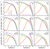 |
Fig. 1. Comparisons between the HIMF of the different simulations and the observations. Solid lines represent the models, and the observations for all galaxies at z ∼ 0 are shown in open purple dots. The results of all the SFGs at z ∼ 1 from Chowdhury et al. (2024) are plotted in dashed lines, and the 1σ errors are indicated by the shaded region. The high-mass range of the HIMF is largely contributed by SFGs; therefore, the SFG results at z ∼ 1 would be similar to those for the entire galaxy population. The top row represents the HIMF for all galaxies, and the middle and bottom rows show the HIMF for the central and satellite galaxies, respectively. Different columns represent different redshifts. |
The results for all star-forming galaxies (SFGs) at z ∼ 1 from Chowdhury et al. (2024) are depicted with dashed lines, while the shaded regions indicate the 1σ errors. Since the HIMF is primarily contributed by the SFGs, the resulting HIMF of the SFGs would be mostly consistent with that of the entire galaxy sample. Chowdhury et al. (2024) combine the B-band luminosity function, Φ(MB), with the MH I-MB measurements at z ∼ 1 to infer the HIMF. They assumed the same measurement error in the MH I-MB relation of  as in the local universe. However, we caution that the conversion from MH I-MB relation at z ∼ 1 to the HIMF would depend on the assumptions in the evolution of the B-band luminosity and the scatter in the MH I-MB relation.
The top left panel clearly shows that most models reasonably represent the observed HIMF at z = 0. The TNG model exhibits a slight excess of H I-rich galaxies at the high-mass end. SIMBA shows a decreasing trend for MH I < 109 M⊙ due to the limited mass resolution (Davé et al. 2020). Therefore, we only focused on galaxies with MH I > 109 M⊙ for SIMBA. The evolution trends of the HIMF vary in different models. In GAEA and TNG, the massive end of HIMF increases as the redshift decreases, whereas the low-mass end of HIMF decreases over time. We confirm that the HIMFs of GAEA at the massive end are not affected by the small simulation volume of MillenniumII. Adopting the GAEA implementation in the Millennium Simulation with a larger box size of 500 Mpc/h produces consistent HIMFs at the massive end. In contrast, there is only weak evolution at the low-mass end in NUM, while the massive end quickly decreases towards z = 0, resulting from the descending trend of ΩH I shown in Figure 2. The evolution of the HIMF in SIMBA shows a relatively minor change, with a slightly higher HIMF at the massive end at higher redshifts.
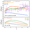 |
Fig. 2. Comparisons between H I fraction, ΩH I(z), from different simulations (solid lines) and observational data (open circles) from Lah et al. (2007), Guimarães et al. (2009), Prochaska & Wolfe (2009), Noterdaeme et al. (2012), Delhaize et al. (2013), Rhee et al. (2013), Zafar et al. (2013), Crighton et al. (2015), Hoppmann et al. (2015), Sánchez-Ramírez et al. (2016), Rao et al. (2017), Bera et al. (2019). For further details, see Table 2 of Walter et al. (2020). The top panel shows all the H I in the galaxies and the IGM with no selection. We refer to Fig. 4 of Guo et al. (2023) for more details about the observations. The bottom panel shows ΩH I of different theoretical models with a mass threshold of M* > 108.5 M⊙ (dashed lines). The labels are the same as in Figure 1. |
However, we note that the observed measurements of HIMF could also suffer from systematic effects, such as the cosmic variance effect at the massive end. The HIMF of Chowdhury et al. (2024) at z ∼ 1 is based on measurements in the small sky area of the DEEP2 survey, which could potentially be affected by the cosmic variance effect. From a simple test of splitting the (250h−1 Mpc)3 volume of the NUM catalogue into 27 subvolumes, we find that the HIMF will change by around 0.2 dex due to the comic variance effect. The HIMF of the ALFALFA survey at z ∼ 0 is based on a much more reliable sample that covers around 7000 square degrees. Moreover, the typical measurement error of the H I mass in ALFALFA is around 0.05 dex, which makes the effect of the Eddington bias minimal.
Most of the existing blind surveys in H I are limited to low redshifts of z < 0.5. As a result, it is challenging to differentiate between various model forecasts regarding the evolution of HIMF. However, recent measurements of HIMF beyond the local universe tend to favour much more H I-rich galaxies at higher redshifts (Xi et al. 2021; Chowdhury et al. 2024). In the middle panels of Figure 1, we show the HIMF measurement of Chowdhury et al. (2024) using Giant Metrewave Radio Telescope (GMRT) observations at z ∼ 1 for SFGs with MH I > 1010 M⊙ as the dashed line, and the corresponding errors are shown as the shaded region. The NUM model is in very good agreement with the measurement of Chowdhury et al. (2024), reproducing the strong evolution of the HIMF at the massive end.
When analysing the contributions to the HIMF by distinguishing between central galaxies (middle panels) and satellite galaxies (bottom panels), it becomes apparent that central galaxies are the primary contributors to the HIMF across all redshifts from 0 to 2, and this pattern is consistent across all models, as already shown in Lagos et al. (2011). This is mainly because the stellar mass functions are higher for central galaxies than for satellites. Gas depletion in satellite galaxies within a high-density halo environment (Brown et al. 2017; Stevens et al. 2019) only has a secondary impact. Similarly to the top panels, the differences among different models become more pronounced at higher redshifts.
3.2. Cosmic H  abundance ΩH I
The ΩH I (i.e. the total H I density in the universe) can be estimated by directly integrating the HIMF in observation (see e.g. Jones et al. 2018) or from the H I column density measurements of damped Lyman-α systems (see e.g. Wolfe et al. 2005). In simulations, we simply calculated the H I fraction as: ΩH I ≡ ρH I/ρc, where ρH I is the density of H I mass, ρc is the critical density at z = 0.
In Figure 2, we compare the various model predictions with the collection of observed measurements (open circles) of Walter et al. (2020) (we refer to Table 2 of Walter et al. (2020) for further details). The top panel illustrates the results for all H I present in galaxies and the intergalactic medium (IGM), represented by solid lines. The bottom panel displays the data after imposing a resolution threshold of M* > 108.5 M⊙, shown as the dashed lines. In the upper panel of Figure 2, we observe that the NUM model fits the observations reasonably well. Consequently, it will serve as a reference for comparisons.
Villaescusa-Navarro et al. (2018) conducted an extensive analysis of H I in TNG, illustrating ΩH I in their Fig. 2. Likewise, Diemer et al. (2019) investigated ΩH I in TNG4, finding a 30% lower ΩH I than that of Villaescusa-Navarro et al. (2018). As shown in Villaescusa-Navarro et al. (2018), the contribution of IGM (gas particles not associated with any subhaloes) to ΩH I in TNG is less than 5% in z < 2 and around 5%–15% at 2 < z < 4, which cannot explain the significant difference. We note that the post-processing of H I and H2 in Diemer et al. (2019) is only applied to galaxies with M* > 2 × 10⁸ M⊙ or MH I > 2 × 10⁸ M⊙, but it is applied for all gas cells in Villaescusa-Navarro et al. (2018). The mass limit in Diemer et al. (2019) leads to the much smaller ΩH I. The different post-processing models only have a minor effect (Diemer et al. 2019). Since the observational measurements of ΩH I include the H I in galaxies and IGM, we employ the results of Villaescusa-Navarro et al. (2018) in the top panel (solid orange line) and only show the TNG results of Diemer et al. (2019) in the bottom panel. Except for the excess at z < 0.5, ΩH I in TNG closely matches those from observations and NUM up to high redshifts in the top panel. We note that the contribution of H I gas in the CGM (beyond the stellar disc) can be very significant for massive galaxies, as shown in Garratt-Smithson et al. (2021) using the EAGLE simulation. Therefore, it is important to include the contribution of the IGM and CGM gas when estimating ΩH I.
In SIMBA, all gas particles in a halo are assigned to the galaxy with the highest Mbaryon/R2. This method identifies H I as ISM even in low-density areas ( , Davé et al. 2020). However, in the absence of a galaxy exceeding the simulation resolution threshold of M* ∼ 108.4 M⊙ (corresponding to about 16 stellar particles, Davé et al. 2019), the gas particles within a halo would not be linked to any galaxy. The resolution effect results in a substantial amount of H I in the IGM for low-mass haloes. The total predicted ΩH I from the SIMBA model (solid red line) aligns with the observations for redshift ranges z < 0.5 and z > 3, but is substantially overestimated for 0.5 < z < 3.
For GAEA, ΩH I is significantly underestimated at most redshifts and only shows agreement with observations at z ∼ 0. As discussed in Yates et al. (2021), most semianalytical models, including GAEA, are limited by the inadequate modelling of H I in IGM and CGM, as well as in sub-resolution haloes. Di Gioia et al. (2020) tried to overcome the resolution effect by using an HOD method to improve the model of H I in low-mass haloes, but it did not improve the model predictions at z > 2. As noted by Spinelli et al. (2020) and Yates et al. (2021), the correction to the sub-resolution haloes is not enough to resolve the differences.
To compare the different models for only well-resolved galaxies, we show in the bottom panel of Figure 2 the results after imposing the stellar mass threshold of M* > 108.5 M⊙. Interestingly, the differences among the theoretical models become smaller because of the removal of a large portion of H I in low-resolution haloes. Compared to the top panel, ΩH I of NUM only decreases by around 20%–30% for z < 2, but decreases sharply at higher redshifts. It emphasises the dominant contribution of H I in low-mass galaxies at high redshifts. Accurate modelling of H I in these galaxies is key to understanding the evolution of ΩH I.
Unlike the top panel, ΩH I of TNG for these well-resolved galaxies is becoming much smaller than that of NUM for z > 0.5. Since the contribution of IGM to ΩH I is still small at these redshifts (Villaescusa-Navarro et al. 2018), it suggests that TNG might underestimate the H I mass in massive galaxies at high redshifts, as will be shown in the following sections. The resolution effect is more severe for SIMBA, with ΩH I decreasing significantly for galaxies above 108.5 M⊙. The predictions of SIMBA get closer to those of NUM for these well-resolved galaxies. Compared to the top panel, ΩH I of GAEA exhibits a minimal shape change. It confirms the previous conclusion that the resolution effect is not the main culprit of the differences.
3.3. Conditional H I mass function
To further investigate the cause of the differences, we calculated the HIMF in halo mass bins ranging from 1010 M⊙ to 1014 M⊙, which is called Conditional HIMF (CHIMF). As in Section 3.1, we used all galaxies within the given mass bins to compute the CHIMFs, applying resolution limits of M* > 106 M⊙ for fair comparison.
We included an additional model at z = 0 from Li et al. (2022), who investigated the CHIMF based on an H I mass estimator that fully utilises the observed galaxy properties. Their H I mass estimator is formulated as the H I-to-stellar mass ratio (log (MH I/M*)), utilising a linear combination of four galaxy parameters: surface stellar mass density (log μ*), colour index (u − r), stellar mass (log M*), and concentration index (log(R90/R50)). Assuming a Gaussian error distribution, they fitted this estimator to the xGASS sample, considering an H I mass threshold of log (MH I/M⊙) > 9.5 due to potential non-detections and incompleteness at the low-mass end. However, they only presented the CHIMF for haloes of Mvir > 1012 M⊙, which are indicated by the purple lines in Figure 3.
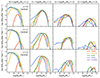 |
Fig. 3. Comparisons between the CHIMF of central galaxies in the different simulations. The labels are the same as in Figure 1. The results of Li et al. (2022) are plotted in solid purple lines. Within the mass interval 12 < log(Mvir/M⊙) < 14, the halo count in GAEA is similar to that in SIMBA, whereas TNG has only about 50% as many as SIMBA. |
Figure 3 displays the CHIMF of central galaxies for various simulations, represented by solid lines of different colours. Each column represents a different range of host halo mass, while each row represents a different redshift. There is a significant decrease in the peaks of the CHIMF as the host halo increases in all redshift ranges, indicating fewer H I-rich galaxies in more massive haloes. This indicates that most H I in the universe is hosted by central galaxies in low-mass haloes of Mvir < 1012 M⊙, which is also consistent with the results of Lagos et al. (2011). The HIMF for MH I < 109 M⊙ is apparently dominated by central galaxies in haloes of Mvir ∼ 1010 − 1011 M⊙, while the high-mass end is mainly contributed by central galaxies with Mvir ∼ 1011 − 1012 M⊙ (see also Lagos et al. 2011). As the redshift decreases to 0, the HIMF increases in the highest halo mass range (Mvir ∼ 1013 − 1014 M⊙). These massive haloes typically have a late formation time and higher probabilities of accumulating H I gas through mergers (Guo et al. 2023).
In general, different theoretical models show similar distributions of CHIMFs for central galaxies at z = 0, but the differences become larger at higher redshifts, as in Figure 1. We note that there is a bimodal distribution in the CHIMF of the central galaxies in the NUM model, particularly in the halo mass range of Mvir ∼ 1012 − 1013 M⊙ at z > 1. It is mainly caused by the bimodal distribution of SFRs in different halo mass bins in the UNIVERSEMACHINE model (Behroozi et al. 2019). This also aligns with the result of Li et al. (2022), where they found that the CHIMFs of red central galaxies peak at lower MH I than those of the blue centrals (their Fig. 7). Interestingly, GAEA tends to predict a much higher H I abundance for low-H I galaxies in massive haloes, which is not seen in other models except for the case of TNG100 in the halo mass bin of 12 < log(Mvir/M⊙) < 13 at z = 0.
Figure 4 shows the CHIMF of satellite galaxies in different redshift and halo mass bins, as in Figure 3. Similarly to central galaxies, the massive end of the satellite HIMF is mostly contributed by galaxies in massive haloes. Different models have similar shapes of satellite CHIMF at the massive end, but they differ significantly for low-H I galaxies. However, since the total HIMF is dominated by central galaxies, these differences in the satellite CHIMF do not have any strong effect on the total HIMF and are thus hard to discriminate in observations.
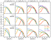 |
Fig. 4. Comparisons between the CHIMF of satellite galaxies from the different simulations. The labels are the same as in Figure 1. Results from Li et al. (2022) are plotted in solid purple lines. Within the mass interval 12 < log(Mvir/M⊙) < 14, the halo count in GAEA is similar to that in SIMBA, whereas TNG has only about 50% as many as SIMBA. |
3.4. H I-halo mass relation
The H I-halo mass relation, denoted as ⟨MH I,tot|Mvir⟩, characterises the total mass of the H I gas (including all member galaxies and the IGM) in haloes of varying virial masses (Mvir) (Guo et al. 2020; Calette et al. 2021; Dev et al. 2023; Rhee et al. 2023). Guo et al. (2020) measured the H I-halo mass relation at z ∼ 0 by selecting haloes from the overlapping areas of ALFALFA and galaxy groups constructed from SDSS DR7 (Lim et al. 2017). Figure 5 shows the total H I-halo mass relation for different simulations and the observations, represented by solid lines and dots, respectively. Each column corresponds to a different redshift. Measurements at z = 0 from Guo et al. (2020) are represented by open purple circles with error bars, and the measurements from Rhee et al. (2023) and Dev et al. (2023) (for haloes with at least two member galaxies) are plotted as purple diamonds and squares, respectively.
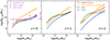 |
Fig. 5. Comparisons between total H I mass and halo mass in the different simulations and the observations. Solid lines and dots represent the models and the observations, respectively. The shaded area represents the 1σ error range calculated with the bootstrapping method. Different columns represent different redshifts. Measurements of the H I-halo mass relation at z = 0 with confusion correction in Guo et al. (2020) are shown as open purple circles, while the measurements from Rhee et al. (2023) and Dev et al. (2023) for haloes with at least two member galaxies are plotted as purple diamonds and squares, respectively. We include all the H I in the galaxies and the IGM as in Figure 2; therefore, we employ the results of Villaescusa-Navarro et al. (2018) for TNG and use H I in haloes for SIMBA. |
Except for TNG100, which overpredicts the total H I mass in massive haloes, all other models show reasonable agreement with the observation at z = 0. By design, the NUM model accurately reproduces the H I-halo mass relation. SIMBA slightly overpredicts MH I,tot in low-mass haloes by around 0.3 dex. As discussed in Ma et al. (2022), the overabundance of H I gas for massive haloes in TNG100 is mainly caused by the kinetic AGN feedback in massive galaxies, which only redistributes the cold gas from the inner stellar disc to the outer region without enough depletion.
The differences among the models become much larger at higher redshifts. The NUM model agrees better with SIMBA at z = 1 and z = 2, where they both predict much more H I gas at high redshifts compared to haloes at z = 0. There is not much evolution in the H I-halo mass relation of TNG100, with only slightly higher H I masses in the most massive haloes at higher redshifts. GAEA shows a comparable amount of H I gas with NUM for Mvir > 1013 M⊙ at all redshifts, but predicts a much smaller MH I,tot for low-mass haloes at z = 1 and z = 2. As we show in Figures 3 and 4, most H I gas in the universe is contained in haloes of Mvir < 1012 M⊙. The lower MH I,tot at the low halo mass end leads to the lower ΩH I in Figure 2. As seen in Figure 3, the CHIMF distributions for GAEA in the halo mass bin of 11 < log(Mvir/M⊙) < 12 peak at much lower MH I values at z > 0 compared to NUM and SIMBA, i.e. the H I gas in these haloes is significantly depleted at higher redshifts. Physically, it might be caused by the efficient consumption of H I gas to support the high SFRs at these redshifts in GAEA and TNG100.
3.5. H I-Stellar mass relation
The H I-stellar mass relation, denoted as ⟨MH I|M*⟩, is another important relation that has been commonly measured in the literature (see e.g. Saintonge & Catinella 2022). Using the H I spectra stacking technique, Guo et al. (2021) accurately measured ⟨MH I|M*⟩ for star-forming and quenched central galaxies (categorised based on SFR) using the same galaxy sample as in Guo et al. (2020). This is particularly crucial for quenched galaxies (QGs), as most of them lack individual 21 cm detections (Catinella et al. 2018). We compared their measurements with model predictions at z = 0 and the H I-stellar mass measurements from Chowdhury et al. (2022) obtained with GMRT at z ∼ 1. At z ∼ 0.37, we adopted the measurements of Rhee et al. (2018) and Bera et al. (2019) from GMRT as well as the measurements of Sinigaglia et al. (2022) from MeerKAT. We focused on the comparisons for SFGs as they are the main targets of observation at high redshifts.
All these observations adopted the H I stacking method to obtain the average H I masses for SFG samples - that is, ⟨MH I⟩. We measured the corresponding H I masses in the same way across the different models, as log(Σi MH I,i/Nhalo,i), where Nhalo, i is the number of host haloes in a given halo mass bin i, and the summation of Σi MH I,i is over all galaxies in the halo mass bin. To ensure fair comparisons, we only considered SFGs with stellar masses in the range of 109 − 1012 M⊙ that can be fully resolved at different simulation resolutions.
For fair comparisons, at z = 0 we adopted the same SFR cut in all models to select star-forming central galaxies as in Guo et al. (2021):

At high redshifts, different SFR cuts are adopted for different simulations. For SIMBA, we followed the definition of the cut that separates SFGs from QGs, as outlined in Davé et al. (2019). This ensures consistency and facilitates a more accurate comparison with the results from Davé et al. (2020) obtained via the expression,

For TNG and GAEA, we first determined the SFMS by fitting a power law relation to the number density peaks of galaxies with specific SFR (sSFR) larger than 10−11yr−1, as in Ma et al. (2022). Then the cuts between the star-forming and QGs were simply set as 1 dex below the SFMS.
The best-fit cuts at different redshifts for TNG are as follows:


Similarly, the cuts for GAEA galaxies are


For NUM galaxies, we followed the same definition of SFMS as in Eq. (5) of Guo et al. (2023) and used the cut as 1 dex below the SFMS. The above cuts do not have a significant impact on our conclusions. All SFR cuts are plotted in dotted red lines (blue dashed lines at z = 0) in Figure 6, the blue points represent the SFGs, and the red points represent the QGs.
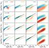 |
Fig. 6. Stellar mass and SFR relation in different simulations at various redshifts. The blue points represent the SFGs, and the red points represent the QGs. The top row shows the relation at z = 0, and the SFR cuts are plotted in dashed blue lines. We use the same SFR cut described in Equation (8) for equal comparison. The rows below show the relation at z = 0.37, 1, and 2, respectively. For SIMBA, TNG and GAEA, the SFR cuts follow the Equations (9)–(12) and are indicated by dotted red lines. As for NUM, we follow the same definition of the SFMS as in Eq. (5) of Guo et al. (2023), and use a cut at 1 dex below the SFMS. |
We note that all stellar masses in the theoretical models and observations in this study adopted the stellar initial mass function of Chabrier (2003). Comparisons between the H I-stellar mass relations in different simulations and observations for SFGs are shown in Figure 7. In this figure, the solid lines and dots represent the models and the observations, respectively. The shaded area represents the 1σ error in the model predictions. Each column in the figure corresponds to a different redshift. For comparisons, we also display the stacked H I measurements in different NUV−r colour bins from Brown et al. (2015) using the ALFALFA sample. The selection cuts in the SFR and NUV−r colour produce different slopes of the H I-stellar mass relations. The star-forming population is nevertheless shown with the NUV−r in the range of [1, 5], consistent with Catinella et al. (2018).
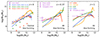 |
Fig. 7. Comparisons between total H I mass and stellar mass of SFGs in the different simulations and the observations. Solid lines and dots represent the models and the observations, respectively. The shaded area represents the 1σ range calculated with bootstrap. TNG100 and GAEA do not have a catalogue at z = 0.37, so we use the catalogue of z = 0.5 instead in the middle panel. Different columns represent different redshifts. The stacked H I-stellar mass results by Guo et al. (2021) are indicated by open purple circles in the left panel, as well as the stacked measurements of Brown et al. (2015) in different NUV−r colour bins (indicated by diamonds with different colours). Measurements of Rhee et al. (2018), Bera et al. (2019), and Sinigaglia et al. (2022) at z ∼ 0.37 are plotted as open circles, diamonds, and squares in the middle panel, respectively. Results of Chowdhury et al. (2022) generated from GMRT at z ∼ 1 are indicated by open purple circles in the right panel. |
At z ∼ 0 (the left panel of Figure 7), SIMBA and GAEA agree reasonably well with the measurement of Guo et al. (2021). GAEA tends to slightly underestimate the H I masses in low-mass central galaxies of M* < 1010 M⊙. This corresponds to the underestimates of HIMF in the mass range of 8.5 < log(MH I/M⊙) < 9.5 seen in Figure 1. Similarly, TNG100 overestimates the H I masses for massive galaxies (as also shown in Fig. 2 of Ma et al. 2022 and Fig. 5 of Stevens et al. 2019), which also causes the overestimates of H I-rich galaxies in the massive end of the HIMF. As discussed in Stevens et al. (2019), the influence of AGN feedback in TNG is weaker for central galaxies, compared to satellite galaxies, because the ejected gas will more likely be re-accreted by the centrals, rather than satellites.
We note that the TNG100 and GAEA simulations do not have the output of H I catalogues at z = 0.37, so we use the catalogues of z = 0.5 in the middle panel instead. The stacked H I measurements of Rhee et al. (2018), Bera et al. (2019), and Sinigaglia et al. (2022) at z ∼ 0.37 are shown as different symbols. Measurements of Chowdhury et al. (2022) at z ∼ 1 are shown as open purple circles in the right panel. The differences among the different models become significantly larger at these higher redshifts. The general trend is consistent with the results in the H I-halo mass relation. TNG100 and GAEA tend to underestimate the H I content in low-mass galaxies, and their redshift evolution of the H I-stellar mass relation is mild. Currently, our ability to observe H I targets at high redshifts is very limited, and most of the available data are around z = 0.37. The large differences between models at higher redshift indicate that HI surveys at higher redshift are essential in constraining galaxy formation models.
In addition, we compare the H I – stellar mass relation for QGs at z = 0 in Figure 8. The results for different models are plotted in solid lines with the same colours as in Figure 7 and are compared to the stacked H I observations of Guo et al. (2021) (purple circles). We find that TNG tends to overestimate the H I in QGs and GAEA tends to underestimate them, while SIMBA fits the observations quite well.
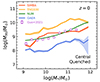 |
Fig. 8. Comparisons between total H I mass and stellar mass of QGs in the different simulations and the observations. Solid lines represent the results obtained with the models, and the shaded area indicates the 1σ range calculated with bootstrap. The stacked H I-stellar mass results obtained by Guo et al. (2021) are indicated by open purple circles with error bars. |
3.6. Halo occupation distribution
To better understand the different H I distributions in the models, it is also helpful to compare the HODs for galaxies with different H I mass thresholds (Guo et al. 2017). The HOD characterises the likelihood distribution P(N|Mvir) for the presence of N galaxies within a specific dark matter halo with virial mass Mvir (see e.g. Jing et al. 1998; Berlind & Weinberg 2002; Zheng et al. 2005; Guo et al. 2015). In principle, the information content of the HOD is the same as that of the CHIMF (Yang et al. 2003). But the HOD provides a straightforward way to understand the distributions of central and satellite galaxies in different haloes (see e.g. Qin et al. 2022).
Figure 9 illustrates the HOD of the various models, with solid lines for central galaxies and dotted lines for satellite galaxies. Each column corresponds to a different H I mass threshold sample as labelled, and each row represents a different redshift. The satellite HODs for galaxies with different MH I thresholds have similar shapes in different models, but with slightly different amplitudes. TNG100 generally predicts more H I-rich satellites than other models, especially for the samples of MH I > 108M⊙. This means that the H I depletion for satellites in TNG100 is not efficient enough for low-mass galaxies.
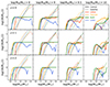 |
Fig. 9. Comparisons of HOD in the different simulations. Solid lines and dotted lines represent the central and satellite galaxies, respectively. Different columns represent different H I mass bins, and different rows represent different redshifts. |
TNG100, SIMBA, and NUM have similar central HODs for low-MH I galaxies. We note that for the sample of MH I > 108M⊙, SIMBA seems to predict a much higher central halo mass cutoff than other models. But in fact it is just caused by the low-mass resolution of the SIMBA simulation. As seen in Figure 1, there are very few galaxies with MH I < 109 M⊙ in SIMBA. Therefore, the HODs of MH I > 108M⊙ and MH I > 109 M⊙ are almost the same in SIMBA because of the lack of low-MH I galaxies.
The central HOD in GAEA approaches unity in haloes of Mvir ∼ 1011 − 1012 M⊙ but begins to decrease for massive haloes. This indicates that central galaxies in more massive haloes are increasingly H I-poor in GAEA. The H I depletion in these central galaxies is more efficient than in other models. This trend is even more prominent in samples with higher H I thresholds. As the H I-stellar mass relation for star-forming central galaxies in GAEA is consistent with that of NUM, it implies that the H I depletion in QGs of GAEA is likely too strong. This cannot be attributed to the low SFRs of these QGs, as indicated by the similar SFR distributions to other models in Figure 6. We confirm this by comparing the stacked H I-stellar mass relation for quenched centrals in Guo et al. (2021) with the corresponding predictions from GAEA and find a 0.7 dex lower MH I for quenched centrals in GAEA, as shown in Figure 8. We also investigate the average H I depletion timescales (MH I/SFR) of QGs in different models, and find that massive QGs in GAEA indeed have much lower H I depletion timescales. These differences will be further investigated in our future work.
4. Discussion
The statistical measurements of H I observations are still very limited, especially beyond the local universe due to the sensitivity limits of radio telescopes. It is therefore very important to have theoretical models that can help us understand the evolutionary history of the cosmic H I content. The motivation of the NUM model is to build an empirical model to successfully describe the available H I measurements without involving complicated baryonic physical processes. Comparisons between NUM and other theoretical models would enhance our understanding of the properties of galaxy H I gas.
The HIMF is well measured with blind H I surveys and robust against observational systematics. For example, the GAEA model is calibrated with the HIMF of Haynes et al. (2011) using the early data release of ALFALFA, which is consistent with the latest HIMF measurement of Guo et al. (2023). Interestingly, neither TNG100 nor SIMBA is tuned to match the HIMF at z ∼ 0, but they show a general agreement with the observation. This might be related to the fact that the model parameters of these simulations are tuned to reproduce the galaxy stellar mass functions and stellar-halo mass relations at z ∼ 0. In the NUM model, the H I mass is mainly determined by the halo mass, the halo formation time, and the SFR. In addition, Chauhan et al. (2020) found that the H I mass can also be influenced by the halo spin parameter and the substructure fraction in the SAM of SHARK (Lagos et al. 2018).
However, HIMF by itself is insufficient to completely distinguish between models, as it only describes the number densities of galaxies with different H I masses. The H I-halo and H I-stellar mass relations are crucial for connecting the H I gas and its host galaxies (haloes). As depicted in Figure 1, the four theoretical models align reasonably well with the observed HIMF at z ∼ 0. TNG100 tends to slightly overestimate the HIMF at the higher mass end, whereas GAEA underestimates the HIMF in the mass range of 8.5 < log(MH I/M⊙) < 9.5 (which is included in the model calibration; see De Lucia et al. 2024). By analysing the H I-stellar mass relations of various models at z = 0, it is evident that these differences arise from the inconsistency with the observed H I-stellar mass relation. This inconsistency is also seen in the HOD distributions, where TNG100 has notably higher central HODs, and GAEA demonstrates lower central HODs for H I-rich galaxies in massive haloes (Figure 9). As shown in Chauhan et al. (2020) and Ma et al. (2022), the main driver of the different H I distributions in the theoretical models is the AGN feedback mechanism. By comparing the stacked H I masses between AGNs and SFGs with the same M* and SFR, Guo et al. (2022) found that the H I depletion from the AGN feedback is much stronger for galaxies with higher SFRs and higher AGN luminosity. Davé et al. (2020) also compared the cold gas distributions in the simulations of TNG100, SIMBA, and EAGLE. They found the same trend of differences in the HIMF as in this study. They concluded that the thermal-based AGN feedback in EAGLE by raising the temperature of gas and the kinetic AGN feedback in SIMBA and TNG will affect the HIMF in different ways.
The H I-halo mass relation provides further insight into understanding the effect of AGN feedback. Baugh et al. (2019) found a dramatic drop in total H I mass in haloes of 11 < log(Mvir/M⊙) < 12 due to the strong suppression of gas cooling from efficient AGN feedback in the GALFORM model. Chauhan et al. (2020) also found a similar level of drop in the H I-halo mass relation at a slightly higher halo mass range in the SHARK model with a different AGN feedback model. As we show in Figure 5, such a strong drop is not seen in the hydrodynamical simulations of TNG100 and SIMBA, nor in the semi-analytical model of GAEA (see also Fig. 5 of Spinelli et al. 2020). Therefore, the H I-halo mass relation can be used to understand the differences between the different AGN feedback mechanisms.
The CHIMF and HOD include more detailed information on the distributions of H I gas in central and satellite galaxies. Li et al. (2022) investigated the CHIMF for the red and blue centrals and found that the CHIMF distributions of the blue centrals are narrower and peak at higher MH I values. This is consistent with the NUM model of the SFR dependence of the H I mass. It is also manifested in the central HOD distributions of different threshold samples MH I in Figure 9, which makes CHIMF and HOD useful statistics for understanding the H I-halo connection.
5. Conclusions
Hydrodynamical simulations and semi-analytical models offer a convenient approach to studying the universe. However, both models are dependent on physical processes and face challenges when it comes to predicting the properties of H I. To address this issue, we employed the empirical model of NUM (Guo et al. 2023), which is built on observations and demonstrates excellent predictive capabilities for H I statistics. In this study, we compared NUM with other models in terms of CHIMF, H I-halo and H I-stellar mass relations, as well as HOD distributions for H I gas. Our main conclusions are summarised below.
(i) All the theoretical models of TNG100, SIMBA, GAEA, and NUM show reasonable agreement with the observed HIMF at z ∼ 0. TNG100 slightly overestimates the massive end of HIMF, whereas GAEA underestimates HIMF in the range of MH I ∼ 108.5−109.5 M⊙. The differences in the models become much larger at higher redshifts of z = 1 and z = 2. The NUM model still presents remarkable agreement with the HIMF measurements of Chowdhury et al. (2024) at z = 1, but other models tend to underestimate the high-mass end of the HIMF at this redshift. The evolutionary trend at the high-mass end is even stronger at z = 2, with NUM predicting much more H I-rich galaxies, SIMBA showing roughly constant number densities, and both TNG100 and GAEA indicating much smaller amplitudes.
(ii) From the comparisons for the CHIMF, it is clear that the HIMF is mainly dominated by central galaxies at all H I masses and redshifts. The low-mass end of the HIMF (MH I < 109 M⊙) is mainly contributed by haloes with 10 < log(Mvir/M⊙) < 11, while the high-mass end is dominated by haloes with 11 < log(Mvir/M⊙) < 12. As in the case of HIMF, the differences in the CHIMF distributions of the models are generally small for central galaxies at z ∼ 0, but become larger at higher redshifts, especially for galaxies in massive haloes. The differences in the satellite CHIMFs are even greater. Future H I surveys of satellite galaxies will provide tighter constraints on different models.
(iii) The differences in the HIMFs of different models can be better understood using the CHIMF and the H I HOD. It is evident in the central H I HOD distributions that TNG100 overpredicts the number of central galaxies with high MH I in massive haloes, and GAEA shows very strong depletion of H I gas in quenched central galaxies of massive haloes. The most likely cause of these differences is the AGN feedback mechanisms implemented in these models, as the main differences lie in the quenched populations in massive haloes.
The linking length is often expressed in units of the mean separation between particles, which is the average distance between particles in the simulation. A common choice for the linking length is 0.2 times the mean interparticle separation. This value was chosen to balance the identification of physically meaningful haloes while avoiding over-merging (grouping unrelated particles).
Corrected measurements of their result are available at http://www.benediktdiemer.com/data/hi-h2-in-illustris/
Acknowledgments
We thank the anonymous reviewer for the constructive report that significantly improves the presentation of this paper. This work is supported by the National SKA Program of China (grant No. 2020SKA0110100), the CAS Project for Young Scientists in Basic Research (No. YSBR-092), the science research grants from the China Manned Space Project with NOs, CMS-CSST-2021-A02 and GHfund C(202407031909). We acknowledge the use of the High Performance Computing Resource in the Core Facility for Advanced Research Computing at the Shanghai Astronomical Observatory.
References
- Adams, E. A. K., Adebahr, B., De Blok, W. J. G., et al. 2022, A&A, 667, A38 [NASA ADS] [CrossRef] [EDP Sciences] [Google Scholar]
- Barnes, D. G., Staveley-Smith, L., de Blok, W. J. G., et al. 2001, MNRAS, 322, 486 [Google Scholar]
- Baugh, C. M., Gonzalez-Perez, V., Lagos, C. d. P., et al. 2019, MNRAS, 483, 4922 [NASA ADS] [CrossRef] [Google Scholar]
- Behroozi, P. S., Wechsler, R. H., & Wu, H.-Y. 2012, ApJ, 762, 109 [Google Scholar]
- Behroozi, P. S., Wechsler, R. H., & Conroy, C. 2013, ApJ, 770, 57 [NASA ADS] [CrossRef] [Google Scholar]
- Behroozi, P., Wechsler, R. H., Hearin, A. P., & Conroy, C. 2019, MNRAS, 488, 3143 [NASA ADS] [CrossRef] [Google Scholar]
- Bera, A., Kanekar, N., Chengalur, J. N., & Bagla, J. S. 2019, ApJ, 882, L7 [NASA ADS] [CrossRef] [Google Scholar]
- Berlind, A. A., & Weinberg, D. H. 2002, ApJ, 575, 587 [Google Scholar]
- Bianchetti, A., Sinigaglia, F., Rodighiero, G., et al. 2025, ApJ, 982, 82 [Google Scholar]
- Bird, S., Garnett, R., & Ho, S. 2016, MNRAS, 466, 2111 [Google Scholar]
- Blitz, L., & Rosolowsky, E. 2006, ApJ, 650, 933 [NASA ADS] [CrossRef] [Google Scholar]
- Boylan-Kolchin, M., Springel, V., White, S. D. M., Jenkins, A., & Lemson, G. 2009, MNRAS, 398, 1150 [Google Scholar]
- Brown, T., Catinella, B., Cortese, L., et al. 2015, MNRAS, 452, 2479 [Google Scholar]
- Brown, T., Catinella, B., Cortese, L., et al. 2017, MNRAS, 466, 1275 [Google Scholar]
- Calette, A. R., Rodríguez-Puebla, A., Avila-Reese, V., & Lagos, C. d. P. 2021, MNRAS, 506, 1507 [NASA ADS] [CrossRef] [Google Scholar]
- Catinella, B., Schiminovich, D., Kauffmann, G., et al. 2010, MNRAS, 403, 683 [Google Scholar]
- Catinella, B., Saintonge, A., Janowiecki, S., et al. 2018, MNRAS, 476, 875 [NASA ADS] [CrossRef] [Google Scholar]
- Chabrier, G. 2003, PASP, 115, 763 [Google Scholar]
- Chauhan, G., Lagos, C. d. P., Stevens, A. R. H., et al. 2020, MNRAS, 498, 44 [Google Scholar]
- Chowdhury, A., Kanekar, N., & Chengalur, J. N. 2022, ApJ, 931, L34 [Google Scholar]
- Chowdhury, A., Kanekar, N., & Chengalur, J. N. 2024, ApJ, 966, L39 [Google Scholar]
- Crain, R. A., Schaye, J., Bower, R. G., et al. 2015, MNRAS, 450, 1937 [NASA ADS] [CrossRef] [Google Scholar]
- Crighton, N. H. M., Murphy, M. T., Prochaska, J. X., et al. 2015, MNRAS, 452, 217 [Google Scholar]
- Davé, R., Thompson, R., & Hopkins, P. F. 2016, MNRAS, 462, 3265 [Google Scholar]
- Davé, R., Anglés-Alcázar, D., Narayanan, D., et al. 2019, MNRAS, 486, 2827 [Google Scholar]
- Davé, R., Crain, R. A., Stevens, A. R. H., et al. 2020, MNRAS, 497, 146 [Google Scholar]
- Delhaize, J., Meyer, M. J., Staveley-Smith, L., & Boyle, B. J. 2013, MNRAS, 433, 1398 [NASA ADS] [CrossRef] [Google Scholar]
- De Lucia, G., & Blaizot, J. 2007, MNRAS, 375, 2 [Google Scholar]
- De Lucia, G., Tornatore, L., Frenk, C. S., et al. 2014, MNRAS, 445, 970 [Google Scholar]
- De Lucia, G., Fontanot, F., Xie, L., & Hirschmann, M. 2024, A&A, 687, A68 [NASA ADS] [CrossRef] [EDP Sciences] [Google Scholar]
- Dev, A., Driver, S. P., Meyer, M., et al. 2023, MNRAS, 523, 2693 [NASA ADS] [CrossRef] [Google Scholar]
- Diemer, B., Stevens, A. R. H., Forbes, J. C., et al. 2018, ApJS, 238, 33 [NASA ADS] [CrossRef] [Google Scholar]
- Diemer, B., Stevens, A. R. H., Lagos, C. d. P., et al. 2019, MNRAS, 487, 1529 [Google Scholar]
- Di Gioia, S., Cristiani, S., De Lucia, G., & Xie, L. 2020, MNRAS, 497, 2469 [Google Scholar]
- Duffy, A. R., Kay, S. T., Battye, R. A., et al. 2012, MNRAS, 420, 2799 [NASA ADS] [Google Scholar]
- Fletcher, T. J., Saintonge, A., Soares, P. S., & Pontzen, A. 2021, MNRAS, 501, 411 [Google Scholar]
- Fontanot, F., De Lucia, G., Hirschmann, M., et al. 2020, MNRAS, 496, 3943 [CrossRef] [Google Scholar]
- Fu, J., Guo, Q., Kauffmann, G., & Krumholz, M. R. 2010, MNRAS, 409, 515 [Google Scholar]
- Fu, J., Kauffmann, G., Huang, M.-L., et al. 2013, MNRAS, 434, 1531 [NASA ADS] [CrossRef] [Google Scholar]
- Garratt-Smithson, L., Power, C., Lagos, C. d. P., et al. 2021, MNRAS, 501, 4396 [Google Scholar]
- Giovanelli, R., Haynes, M. P., Kent, B. R., et al. 2005, ApJ, 130, 2598 [Google Scholar]
- Guimarães, R., Petitjean, P., de Carvalho, R. R., et al. 2009, A&A, 508, 133 [Google Scholar]
- Guo, H., Zheng, Z., Zehavi, I., et al. 2015, MNRAS, 453, 4368 [Google Scholar]
- Guo, H., Li, C., Zheng, Z., et al. 2017, ApJ, 846, 61 [NASA ADS] [CrossRef] [Google Scholar]
- Guo, H., Jones, M. G., Haynes, M. P., & Fu, J. 2020, ApJ, 894, 92 [NASA ADS] [CrossRef] [Google Scholar]
- Guo, H., Jones, M. G., Wang, J., & Lin, L. 2021, ApJ, 918, 53 [NASA ADS] [CrossRef] [Google Scholar]
- Guo, H., Jones, M. G., & Wang, J. 2022, ApJ, 933, L12 [NASA ADS] [CrossRef] [Google Scholar]
- Guo, H., Wang, J., Jones, M. G., & Behroozi, P. 2023, ApJ, 955, 57 [NASA ADS] [CrossRef] [Google Scholar]
- Haynes, M. P., Giovanelli, R., Martin, A. M., et al. 2011, ApJ, 142, 170 [Google Scholar]
- Henriques, B. M. B., White, S. D. M., Thomas, P. A., et al. 2015, MNRAS, 451, 2663 [Google Scholar]
- Hirschmann, M., De Lucia, G., & Fontanot, F. 2016, MNRAS, 461, 1760 [Google Scholar]
- Hopkins, P. F. 2017, arXiv e-prints [arXiv:1712.01294] [Google Scholar]
- Hoppmann, L., Staveley-Smith, L., Freudling, W., et al. 2015, MNRAS, 452, 3726 [NASA ADS] [CrossRef] [Google Scholar]
- Huang, S., Haynes, M. P., Giovanelli, R., & Brinchmann, J. 2012, ApJ, 756, 113 [Google Scholar]
- Hutchens, Z. L., Kannappan, S. J., Hess, K. M., et al. 2025, ApJ, 985, 228 [Google Scholar]
- Jing, Y. P., Mo, H. J., & Börner, G. 1998, ApJ, 494, 1 [NASA ADS] [CrossRef] [Google Scholar]
- Jones, M. G., Haynes, M. P., Giovanelli, R., & Moorman, C. 2018, MNRAS, 477, 2 [Google Scholar]
- Kanekar, N., Sethi, S., & Dwarakanath, K. S. 2016, ApJ, 818, L28 [Google Scholar]
- Kennicutt, R. C., Jr 1998, ApJ, 498, 541 [Google Scholar]
- Klypin, A., Yepes, G., Gottlöber, S., Prada, F., & Heß, S. 2016, MNRAS, 457, 4340 [Google Scholar]
- Krumholz, M. R. 2013, MNRAS, 436, 2747 [CrossRef] [Google Scholar]
- Krumholz, M. R., & Gnedin, N. Y. 2011, ApJ, 729, 36 [Google Scholar]
- Lagos, C. D. P., Baugh, C. M., Lacey, C. G., et al. 2011, MNRAS, 418, 1649 [CrossRef] [Google Scholar]
- Lagos, C. d. P., Crain, R. A., Schaye, J., et al. 2015, MNRAS, 452, 3815 [NASA ADS] [CrossRef] [Google Scholar]
- Lagos, C. d. P., Tobar, R. J., Robotham, A. S. G., et al. 2018, MNRAS, 481, 3573 [CrossRef] [Google Scholar]
- Lah, P., Chengalur, J. N., Briggs, F. H., et al. 2007, MNRAS, 376, 1357 [Google Scholar]
- Li, X., Li, C., Mo, H. J., Xiao, T., & Wang, J. 2022, ApJ, 941, 48 [Google Scholar]
- Li, Z., Wolz, L., Guo, H., Cunnington, S., & Mao, Y. 2024, MNRAS, 534, 1801 [Google Scholar]
- Lim, S. H., Mo, H. J., Lu, Y., Wang, H., & Yang, X. 2017, MNRAS, 470, 2982 [NASA ADS] [CrossRef] [Google Scholar]
- Ma, W., Liu, K., Guo, H., et al. 2022, ApJ, 941, 205 [NASA ADS] [CrossRef] [Google Scholar]
- Ma, W., Guo, H., & Jones, M. G. 2025a, A&A, 695, A5 [NASA ADS] [CrossRef] [EDP Sciences] [Google Scholar]
- Ma, W., Guo, H., Xu, H., et al. 2025b, A&A, 695, A241 [NASA ADS] [CrossRef] [EDP Sciences] [Google Scholar]
- Marinacci, F., Vogelsberger, M., Pakmor, R., et al. 2018, MNRAS, 480, 5113 [NASA ADS] [Google Scholar]
- Masui, K. W., Switzer, E. R., Banavar, N., et al. 2013, ApJ, 763, L20 [Google Scholar]
- Meyer, M. J., Zwaan, M. A., Webster, R. L., et al. 2004, MNRAS, 350, 1195 [Google Scholar]
- Naiman, J. P., Pillepich, A., Springel, V., et al. 2018, MNRAS, 477, 1206 [Google Scholar]
- Neeleman, M., Prochaska, J. X., Ribaudo, J., et al. 2016, ApJ, 818, 113 [Google Scholar]
- Nelson, D., Pillepich, A., Springel, V., et al. 2018, MNRAS, 475, 624 [Google Scholar]
- Nelson, D., Springel, V., Pillepich, A., et al. 2019, Comput. Astrophys. Cosmol., 6, 2 [Google Scholar]
- Noterdaeme, P., Petitjean, P., Ledoux, C., & Srianand, R. 2009, A&A, 505, 1087 [NASA ADS] [CrossRef] [EDP Sciences] [Google Scholar]
- Noterdaeme, P., Petitjean, P., Carithers, W. C., et al. 2012, A&A, 547, L1 [NASA ADS] [CrossRef] [EDP Sciences] [Google Scholar]
- Péroux, C., McMahon, R. G., Storrie-Lombardi, L. J., & Irwin, M. J. 2003, MNRAS, 346, 1103 [Google Scholar]
- Pillepich, A., Springel, V., Nelson, D., et al. 2018, MNRAS, 473, 4077 [Google Scholar]
- Planck Collaboration XIII. 2016, A&A, 594, A13 [NASA ADS] [CrossRef] [EDP Sciences] [Google Scholar]
- Popesso, P., Concas, A., Cresci, G., et al. 2023, MNRAS, 519, 1526 [Google Scholar]
- Popping, G., Behroozi, P. S., & Peeples, M. S. 2015, MNRAS, 449, 477 [NASA ADS] [CrossRef] [Google Scholar]
- Prochaska, J. X., & Wolfe, A. M. 2009, ApJ, 696, 1543 [Google Scholar]
- Prochaska, J. X., Herbert-Fort, S., & Wolfe, A. M. 2005, ApJ, 635, 123 [NASA ADS] [CrossRef] [Google Scholar]
- Qin, F., Howlett, C., Stevens, A. R. H., & Parkinson, D. 2022, ApJ, 937, 113 [Google Scholar]
- Rahmati, A., Pawlik, A. H., Raičević, M., & Schaye, J. 2013, MNRAS, 430, 2427 [NASA ADS] [CrossRef] [Google Scholar]
- Rao, S. M., Turnshek, D. A., Sardane, G. M., & Monier, E. M. 2017, MNRAS, 471, 3428 [Google Scholar]
- Rhee, J., Zwaan, M. A., Briggs, F. H., et al. 2013, MNRAS, 435, 2693 [NASA ADS] [CrossRef] [Google Scholar]
- Rhee, J., Lah, P., Briggs, F. H., et al. 2018, MNRAS, 473, 1879 [NASA ADS] [CrossRef] [Google Scholar]
- Rhee, J., Meyer, M., Popping, A., et al. 2023, MNRAS, 518, 4646 [Google Scholar]
- Saintonge, A., & Catinella, B. 2022, ARA&A, 60, 319 [NASA ADS] [CrossRef] [Google Scholar]
- Saintonge, A., Catinella, B., Tacconi, L. J., et al. 2017, ApJS, 233, 22 [Google Scholar]
- Sánchez-Ramírez, R., Ellison, S. L., Prochaska, J. X., et al. 2016, MNRAS, 456, 4488 [Google Scholar]
- Schaye, J., Crain, R. A., Bower, R. G., et al. 2014, MNRAS, 446, 521 [Google Scholar]
- Sinigaglia, F., Rodighiero, G., Elson, E., et al. 2022, ApJ, 935, L13 [NASA ADS] [CrossRef] [Google Scholar]
- Spinelli, M., Zoldan, A., De Lucia, G., Xie, L., & Viel, M. 2020, MNRAS, 493, 5434 [NASA ADS] [CrossRef] [Google Scholar]
- Springel, V. 2010, MNRAS, 401, 791 [Google Scholar]
- Springel, V., & Hernquist, L. 2003, MNRAS, 339, 289 [Google Scholar]
- Springel, V., White, S. D. M., Tormen, G., & Kauffmann, G. 2001, MNRAS, 328, 726 [Google Scholar]
- Springel, V., Pakmor, R., Pillepich, A., et al. 2018, MNRAS, 475, 676 [Google Scholar]
- Stevens, A. R. H., Diemer, B., Lagos, C. d. P., et al. 2019, MNRAS, 483, 5334 [NASA ADS] [CrossRef] [Google Scholar]
- Tacconi, L. J., Genzel, R., & Sternberg, A. 2020, ARA&A, 58, 157 [NASA ADS] [CrossRef] [Google Scholar]
- Villaescusa-Navarro, F., Genel, S., Castorina, E., et al. 2018, ApJ, 866, 135 [NASA ADS] [CrossRef] [Google Scholar]
- Walter, F., Brinks, E., de Blok, W. J. G., et al. 2008, ApJ, 136, 2563 [Google Scholar]
- Walter, F., Carilli, C., Neeleman, M., et al. 2020, ApJ, 902, 111 [Google Scholar]
- Wolfe, A. M., Gawiser, E., & Prochaska, J. X. 2005, ARA&A, 43, 861 [NASA ADS] [CrossRef] [Google Scholar]
- Xi, H., Staveley-Smith, L., For, B.-Q., et al. 2021, MNRAS, 501, 4550 [NASA ADS] [Google Scholar]
- Xie, L., De Lucia, G., Hirschmann, M., Fontanot, F., & Zoldan, A. 2017, MNRAS, 469, 968 [Google Scholar]
- Xie, L., De Lucia, G., Hirschmann, M., & Fontanot, F. 2020, MNRAS, 498, 4327 [NASA ADS] [CrossRef] [Google Scholar]
- Xie, L., De Lucia, G., Fontanot, F., et al. 2024, ApJ, 966, L2 [NASA ADS] [CrossRef] [Google Scholar]
- Yang, X., Mo, H. J., & van den Bosch, F. C. 2003, MNRAS, 339, 1057 [Google Scholar]
- Yates, R. M., Péroux, C., & Nelson, D. 2021, MNRAS, 508, 3535 [NASA ADS] [CrossRef] [Google Scholar]
- Zafar, T., Péroux, C., Popping, A., et al. 2013, A&A, 556, A141 [NASA ADS] [CrossRef] [EDP Sciences] [Google Scholar]
- Zhang, C.-P., Zhu, M., Jiang, P., et al. 2024, Sci. China Phys. Mech. Astron., 67, 219511 [NASA ADS] [CrossRef] [Google Scholar]
- Zheng, Z., Berlind, A. A., Weinberg, D. H., et al. 2005, ApJ, 633, 791 [NASA ADS] [CrossRef] [Google Scholar]
All Figures
|
Fig. 1. Comparisons between the HIMF of the different simulations and the observations. Solid lines represent the models, and the observations for all galaxies at z ∼ 0 are shown in open purple dots. The results of all the SFGs at z ∼ 1 from Chowdhury et al. (2024) are plotted in dashed lines, and the 1σ errors are indicated by the shaded region. The high-mass range of the HIMF is largely contributed by SFGs; therefore, the SFG results at z ∼ 1 would be similar to those for the entire galaxy population. The top row represents the HIMF for all galaxies, and the middle and bottom rows show the HIMF for the central and satellite galaxies, respectively. Different columns represent different redshifts. |
| In the text | |
|
Fig. 2. Comparisons between H I fraction, ΩH I(z), from different simulations (solid lines) and observational data (open circles) from Lah et al. (2007), Guimarães et al. (2009), Prochaska & Wolfe (2009), Noterdaeme et al. (2012), Delhaize et al. (2013), Rhee et al. (2013), Zafar et al. (2013), Crighton et al. (2015), Hoppmann et al. (2015), Sánchez-Ramírez et al. (2016), Rao et al. (2017), Bera et al. (2019). For further details, see Table 2 of Walter et al. (2020). The top panel shows all the H I in the galaxies and the IGM with no selection. We refer to Fig. 4 of Guo et al. (2023) for more details about the observations. The bottom panel shows ΩH I of different theoretical models with a mass threshold of M* > 108.5 M⊙ (dashed lines). The labels are the same as in Figure 1. |
| In the text | |
|
Fig. 3. Comparisons between the CHIMF of central galaxies in the different simulations. The labels are the same as in Figure 1. The results of Li et al. (2022) are plotted in solid purple lines. Within the mass interval 12 < log(Mvir/M⊙) < 14, the halo count in GAEA is similar to that in SIMBA, whereas TNG has only about 50% as many as SIMBA. |
| In the text | |
|
Fig. 4. Comparisons between the CHIMF of satellite galaxies from the different simulations. The labels are the same as in Figure 1. Results from Li et al. (2022) are plotted in solid purple lines. Within the mass interval 12 < log(Mvir/M⊙) < 14, the halo count in GAEA is similar to that in SIMBA, whereas TNG has only about 50% as many as SIMBA. |
| In the text | |
|
Fig. 5. Comparisons between total H I mass and halo mass in the different simulations and the observations. Solid lines and dots represent the models and the observations, respectively. The shaded area represents the 1σ error range calculated with the bootstrapping method. Different columns represent different redshifts. Measurements of the H I-halo mass relation at z = 0 with confusion correction in Guo et al. (2020) are shown as open purple circles, while the measurements from Rhee et al. (2023) and Dev et al. (2023) for haloes with at least two member galaxies are plotted as purple diamonds and squares, respectively. We include all the H I in the galaxies and the IGM as in Figure 2; therefore, we employ the results of Villaescusa-Navarro et al. (2018) for TNG and use H I in haloes for SIMBA. |
| In the text | |
|
Fig. 6. Stellar mass and SFR relation in different simulations at various redshifts. The blue points represent the SFGs, and the red points represent the QGs. The top row shows the relation at z = 0, and the SFR cuts are plotted in dashed blue lines. We use the same SFR cut described in Equation (8) for equal comparison. The rows below show the relation at z = 0.37, 1, and 2, respectively. For SIMBA, TNG and GAEA, the SFR cuts follow the Equations (9)–(12) and are indicated by dotted red lines. As for NUM, we follow the same definition of the SFMS as in Eq. (5) of Guo et al. (2023), and use a cut at 1 dex below the SFMS. |
| In the text | |
|
Fig. 7. Comparisons between total H I mass and stellar mass of SFGs in the different simulations and the observations. Solid lines and dots represent the models and the observations, respectively. The shaded area represents the 1σ range calculated with bootstrap. TNG100 and GAEA do not have a catalogue at z = 0.37, so we use the catalogue of z = 0.5 instead in the middle panel. Different columns represent different redshifts. The stacked H I-stellar mass results by Guo et al. (2021) are indicated by open purple circles in the left panel, as well as the stacked measurements of Brown et al. (2015) in different NUV−r colour bins (indicated by diamonds with different colours). Measurements of Rhee et al. (2018), Bera et al. (2019), and Sinigaglia et al. (2022) at z ∼ 0.37 are plotted as open circles, diamonds, and squares in the middle panel, respectively. Results of Chowdhury et al. (2022) generated from GMRT at z ∼ 1 are indicated by open purple circles in the right panel. |
| In the text | |
|
Fig. 8. Comparisons between total H I mass and stellar mass of QGs in the different simulations and the observations. Solid lines represent the results obtained with the models, and the shaded area indicates the 1σ range calculated with bootstrap. The stacked H I-stellar mass results obtained by Guo et al. (2021) are indicated by open purple circles with error bars. |
| In the text | |
|
Fig. 9. Comparisons of HOD in the different simulations. Solid lines and dotted lines represent the central and satellite galaxies, respectively. Different columns represent different H I mass bins, and different rows represent different redshifts. |
| In the text | |
Current usage metrics show cumulative count of Article Views (full-text article views including HTML views, PDF and ePub downloads, according to the available data) and Abstracts Views on Vision4Press platform.
Data correspond to usage on the plateform after 2015. The current usage metrics is available 48-96 hours after online publication and is updated daily on week days.
Initial download of the metrics may take a while.