| Issue |
A&A
Volume 695, March 2025
|
|
|---|---|---|
| Article Number | A73 | |
| Number of page(s) | 23 | |
| Section | Astrophysical processes | |
| DOI | https://doi.org/10.1051/0004-6361/202452373 | |
| Published online | 10 March 2025 | |
A multi-ion non-equilibrium solver for ionised astrophysical plasmas with arbitrary elemental abundances
1
Astronomy & Astrophysics Section, School of Cosmic Physics, Dublin Institute for Advanced Studies, DIAS Dunsink Observatory, Dublin 15, Ireland
2
Institute of Astronomy, University of Cambridge, Madingley Rd, Cambridge CB3 0HA, UK
3
Astronomy Unit, School of Physics and Astronomy, Queen Mary University of London, London E1 4NS, UK
4
Department of Astronomy and Oskar Klein Centre, AlbaNova, Stockholm University, SE-10691 Stockholm, Sweden
⋆ Corresponding author; arun@cp.dias.ie
Received:
26
September
2024
Accepted:
31
January
2025
Context. While many astrophysical plasmas can be modelled successfully assuming ionisation and thermal equilibrium, in some cases this is not appropriate and a non-equilibrium approach is required. In nebulae around evolved stars, the local elemental abundances may also strongly vary in space and time.
Aims. Here we present a non-equilibrium multi-ion module developed for the fluid-dynamics code PION, describing the physical processes included and demonstrating its capabilities with some test calculations.
Methods. A non-equilibrium ionisation solver is developed that allows arbitrary elemental abundances for neutral and ionised (but not molecular) gas, for the elements H, He, C, N, O, Ne, Si, S, and Fe. Collisional ionisation and recombination, photoionisation and charge-exchange reactions are included, and ion-by-ion non-equilibrium radiative cooling is calculated based on the instantaneous ion fractions of each element. Element and ion mass-fractions are advected using passive scalars, operator-split from the microphysical processes.
Results. The module is validated by comparing with equilibrium and non-equilibrium calculations in the literature. Effects of charge exchange on ion abundances in cooling plasmas are discussed. Application to modelling shocks and photo-ionised H II regions is demonstrated. The time-dependent expansion of a WR nebula is studied, including photoionisation and collisional processes, and spectral-line luminosities calculated for non-equilibrium and equilibrium plasma states.
Conclusions. The multi-ion module enables simulation of ionised plasmas with spatially varying elemental abundances using self-consistent ion abundances and thermal evolution. This allows prediction of spectral lines in UV, optical, IR, and X-ray even in cases where the plasma is out of ionisation equilibrium.
Key words: astroparticle physics / hydrodynamics / radiative transfer / shock waves / methods: numerical / stars: winds / outflows
© The Authors 2025
 Open Access article, published by EDP Sciences, under the terms of the Creative Commons Attribution License (https://creativecommons.org/licenses/by/4.0), which permits unrestricted use, distribution, and reproduction in any medium, provided the original work is properly cited.
This article is published in open access under the Subscribe to Open model. Subscribe to A&A to support open access publication.
1. Introduction
Hydrodynamic (HD) and magnetohydrodynamic (MHD) simulation has proven to be an essential tool in the understanding of circumstellar nebulae around stars, from pioneering early work on expansion of H II regions (Lasker 1966) to models of Wolf-Rayet (WR) nebulae (García-Segura et al. 1996), colliding-wind binaries (Parkin et al. 2011) and novae (Booth et al. 2016). The thermal state of the gas can be crudely approximated by either an adiabatic or isothermal equation of state in the simplest cases, but often a more detailed approach is required. The cooling timescale, τc = E/Ė (where E is the thermal energy density), by radiative processes is typically driven by electron-ion collisions for which Ė depends on the density, ρ, according to Ė ∝ ρ2, resulting in τc ∝ ρ−1. Dense regions of plasma may have short τc and low-density regions long τc, meaning that within a single simulation one may have adiabatic regions, isothermal regions and intermediate regimes. Most research in the literature addresses this problem using tabulated cooling curves that assume collisional ionisation equilibrium (CIE, e.g. Sutherland & Dopita 1993) or photoionisation equilibrium (PIE, Wiersma et al. 2009), but in some environments this may be a poor assumption.
In particular for molecular clouds, the formation timescales of molecules may be much longer than the dynamical timescale of the gas, and so non-equilibrium chemistry models have been developed with varying degrees of complexity (e.g. Nelson & Langer 1997; Glover & Mac Low 2007; Walch et al. 2015; Gong et al. 2017). The aims of these models are twofold: the chemical state of the gas partially determines its radiative heating and cooling rate, and so a correctly calculated thermal state (with associated hydrodynamical effects from pressure gradients) depends on the non-equilibrium chemistry. Furthermore, predictions for observables such as molecular line-emission depend crucially on how accurately the molecule abundances are calculated.
In ionised plasmas, the ionisation and recombination processes are generally much faster than molecule formation, and so CIE or PIE is often, but not always, a reasonable assumption. Raga et al. (1997) developed a limited non-equilibrium ionisation-cooling model to study bow shocks, showing that multi-dimensional simulations were feasible with this approach, at least without including radiative transfer. Teşileanu et al. (2008) introduced a comprehensive non-equilibrium cooling model to PLUTO (Mignone et al. 2007), showing the importance of non-equilibrium effects in the radiative shocks of protostellar jets, especially for predicting spectral line intensities of commonly observed ions. de Avillez & Breitschwerdt (2012) showed that, for simulations of the multiphase interstellar medium (ISM), the cooling timescales are often shorter than recombination timescales and so a significant fraction of the ISM volume may be quite far from CIE conditions. This has consequences for radiative cooling rates, and hence for the gas dynamics and plasma line-emission, that cannot be captured by a tabulated equilibrium cooling curve. In situations where we may expect the gas to be far from CIE conditions, one cannot make meaningful predictions without explicitly tracking the ionisation state of the observational tracer that we are interested in modelling.
A further complication in nebulae around evolved stars is that the elemental abundances in the stellar wind may change significantly on the dynamical timescale of the nebula, and for binary systems the winds of the two stars may have dramatically different abundances (e.g. Pollock et al. 2005). This makes a tabulated non-equilibrium cooling prescription similar to that of Teşileanu et al. (2008) more difficult to implement because the elemental abundances themselves are now functions of positions and time. Eatson et al. (2022a) calculated tabulated CIE cooling curves appropriate for the surface elemental abundances of the two stars in the binary system WR 140, and used a passive scalar to distinguish the two winds and apply the appropriate cooling rates. This method was applied to study WR 140 in Eatson et al. (2022b) and Mackey et al. (2023) to model the transition from adiabatic to radiative shocks as the stars approach each other around periastron. The issue of variable elemental abundances is also important for simulations of galaxy formation and evolution where gas enrichment and metallicity-dependent cooling are included, and in general for circumgalactic and intergalactic gas. In this context Wiersma et al. (2009) introduced tabulated cooling functions assuming PIE and CIE conditions, computed on an element-by-element basis, accounting for variations in relative elemental abundances. These detailed element-by-element equilibrium cooling functions were implemented in hydrodynamical cosmological simulations such as the EAGLE suite (Schaye et al. 2015), and have been useful in advancing our understanding of galaxy formation and the intergalactic medium.
Frank & Mellema (1994) developed a method for modelling the gas dynamics of photoionised and collisionally ionised plasmas, applied to planetary nebulae. This non-equilibrium method allowed for specifying elemental abundances and was used by Mellema (1995) to study the expansion of Planetary Nebulae, including comparison of synthetic spectral line emission from simulations with observed nebulae. Mellema & Lundqvist (2002) developed this code further to investigate the 1D (spherically symmetric) expansion of circumstellar nebulae for plasmas with very different elemental abundances. They solved the non-equilibrium abundances of a large set of ions, with associated radiative cooling on an ion-by-ion basis, and studied the effect this has on the shock properties and hydrodynamical evolution of the nebulae. For WR nebulae, they found a significant effect of the elemental abundances on gas dynamics. The C2-ray method (Mellema et al. 2006) introduced a method (building on work by Abel et al. 1999) for accurately modelling photoionisation with simulations where cells may have large optical depths. A modified version of this method was used by Mackey (2012) with an explicit integration scheme for the radiation-MHD (R-MHD) code PION. C2-ray was extended by Friedrich et al. (2012) to hard radiation fields capable of singly and doubly ionising helium, but only applied to metal-poor or free gas.
Gnat & Sternberg (2007) investigated cooling and ionisation in low-density gas in the equilibrium and non-equilibrium regimes finding that, in high-metallicity environments, short cooling times lead to significant departures from ionisation equilibrium in cooling gas. Inclusion of photoionisation Gnat (2017) was shown to generally produce gas with ionic cooling rates close to those obtained assuming photoionisation equilibrium for strong radiation fields, and these collisional and photoionisation processes were include as a module for the PLUTO code by Sarkar et al. (2021), although with radiative transfer limited to 1D spherically symmetric calculations. Another non-equilibrium chemical model developed by Oppenheimer & Schaye (2013), demonstrated the important role of low-ionisation states in the circumgalactic medium and the warm and hot ISM, and the significance of non-equilibrium effects mitigated by an extragalactic UV background. Enhancements to this model, including molecular chemistry, dust-grain reactions and shielding radiation in the CHIMES chemistry module (Richings et al. 2014a,b) enable detailed simulations of the multiphase ISM of galaxies (e.g. Richings & Schaye 2016).
Codes that model HD or MHD generally have relatively simple photoionisation schemes because of the large computational cost of multi-frequency radiative transfer and large ionisation networks. By contrast, R-MHD codes that employ Monte-Carlo radiative-transfer such as TORUS (Harries et al. 2019) and CMACIONIZE (Vandenbroucke & Wood 2018) have detailed radiation transport and photoionisation schemes, and may be run in equilibrium or non-equilibrium modes. Although Monte-Carlo radiative transfer scales very efficiently (Harries et al. 2019) these capabilities come at significant computational cost because large numbers of photon packets are required at each time-step to give accurate results.
An important consideration for a multi-ion module including photoionisation and spatially varying elemental abundances, is that it is far from simple to construct a general equilibrium solution (neither CIE nor PIE) because the number of variables that determine the ionisation state may be quite large: density, temperature, elemental abundances, radiation flux in each frequency bin and optical depth of the grid zone being integrated. In this case it may be simpler (and potentially faster) to compute a time-dependent solution. There exist some popular chemistry solvers in the literature suitable for modelling ionised plasmas, for example KROME (Grassi et al. 2014) and GRACKLE (Smith et al. 2017) but there are practical and design drawbacks to using these in PION. GRACKLE is aimed mainly at the high-redshift Universe and its photoionisation capabilities do not extend to multi-ion non-equilibrium ionisation of metals. KROME could in principle be used because it has methods for multi-frequency radiation fields and photoionisation of metals, but it is written in Fortran without a C++ interface. Given that we already had the SUNDIALS ODE solver (Hindmarsh et al. 2005; Gardner et al. 2022) integrated into PION for simpler microphysics modules, we decided to extend this and write our own multi-ion module to calculate and solve the rate equations.
In this paper our aim is to develop and test a non-equilibrium multi-ion module for ionised plasmas in the radiation-MHD code PION (Mackey et al. 2021), including collisional and photoionisation processes, and allowing spatial and temporal variations in elemental abundances. The module can potentially be used in many contexts from large scale simulations of galaxy formation down to au-scale simulations of colliding-wind binary systems. The main applications we aim for are binary systems, WR nebulae and supernova remnants. During peer review of this paper, we became aware of the CHIMES chemistry module (Richings et al. 2014a,b) which shares a number of design similarities to our module, although it has a stronger focus on low-temperature gas that may be partially ionised or molecular.
In Sect. 2, we review the previous microphysics module implemented in PION, followed by a detailed description of the new multi-ion model, emphasizing its advanced features and improvements. Section 3 presents several one-dimensional MHD shock models with different flow properties, resolution, and physical processes. The accuracy of our multi-ion photoionisation scheme is also verified by simulating HII regions and integrating to PIE in Sect. 3.4, comparing results with literature benchmarks. An application of the multi-ion module is presented in Sect. 4, where we model the interaction between fast and slow winds, each having distinct chemical compositions and incorporating all the physical processes discussed in this work. In Sect. 5, we discuss the computational efficiency and performance of the multi-ion module in relation to the number of chemical species and OpenMP threads, and compare equilibrium vs. non-equilibrium solutions for wind-wind interaction, and in Sect. 6, we present our conclusions.
2. Methods
The multi-ion module is developed for PION, an HD and MHD grid-based simulation code with static mesh-refinement, that incorporates radiative transfer of ionising and non-ionising photons for R-HD (Mackey & Lim 2010) and R-MHD (Mackey & Lim 2011). The first public release and description of numerical methods in PION is described in Mackey et al. (2021). The pre-existing microphysics routines in PION assume one of the following:
-
CIE with Solar abundances scaled by a metallicity, and with optional heating terms for UV heating in photo-ionised gas.
-
CIE for a gas composed of two different elemental abundances (distinguished by a passive tracer) with different tabulated cooling rates (Mackey et al. 2023).
-
Non-equilibrium ionisation calculation of hydrogen based on collisional ionisation and photoionisation, and radiative cooling appropriate for atomic and partially ionised gas in the diffuse ISM (Mackey et al. 2013), denoted MPv3.
-
As above, but with low-temperature cooling appropriate for denser gas (Mackey et al. 2015) (see also Henney et al. 2009), denoted MPv5.
-
Two-temperature isothermal model, where neutral gas is isothermal with a low temperature and photo-ionised gas also isothermal with a higher temperature. This model was used for the STARBENCH tests in Bisbas et al. (2015), denoted MPv7.
These microphysics modules have been used successfully to model both photo-ionised and collisionally ionised plasmas around massive stars, but have a strong limitation that the elemental abundances are assumed to be uniform throughout the domain and unchanging in time. Furthermore the ionisation states of important diagnostic ions such as O+, O2+ and others, cannot be calculated without detailed post-processing, assuming either CIE or PIE. This limits the predictive power of simulations using these modules, especially for making synthetic observations, and motivates us to develop the multi-ion non-equilibrium module.
In Sect. 2.1 we describe the physical processes and equations solved by the new microphysics module, dubbed NEMO. Section 2.2 lists the sources for collisional ionisation and recombination rates, checking that CIE abundances agree with literature results. In Sect. 2.3 we derive the CIE cooling functions, comparing our results with established findings to confirm the accuracy of our approach. Sections 2.4 and 2.5 provide detailed descriptions of the photoionisation and charge-exchange schemes.
2.1. New non-equilibrium microphysics module, NEMO
The features and the scope of the newly added non-equilibrium ionisation network and cooling function to the PION code are described below. We begin with the ideal inviscid MHD equations:
![$$ \begin{aligned} \frac{\partial E}{\partial t} + \nabla \cdot \left[\left(E + p + \frac{|\boldsymbol{B}|^2}{2} \right)\boldsymbol{v} - \left(\boldsymbol{v}\cdot \boldsymbol{B}\right)\boldsymbol{B}\right]&= S_E, \end{aligned} $$](/articles/aa/full_html/2025/03/aa52373-24/aa52373-24-eq4.gif)
where the source term SE includes radiative cooling and photo-heating.
The ion abundances of H, He, C, N, O, Ne, Si, S, and Fe are included using passive scalars, Xκ, i, that obey the usual conservation equation:
where the scalar quantity Xκ, i is the mass fraction of the i-th ion of the element κ. The ion abundances for each element satisfy  , where Z is the atomic number of element κ, and the mass fraction of the bare ion Xκ, Z is determined by a conservation equation. For elemental abundances, Xκ, the initial conditions are constrained such that ∑κXκ = 1 everywhere. In terms of ion abundances, this gives
  .
.
The source term Sκ, i represents ionisation and recombination into and out of ionisation state i, and this is evaluated by operator splitting. The homogeneous part of the equations (advection) are solved together with the hydrodynamics, and the source term is solved in the new microphysics module, by time-integrating the rate equations for each ion together with the thermal energy density in each cell. This coupled system of ODEs is solved using the CVODE solver (Cohen et al. 1996) from the SUNDIALS library (Hindmarsh et al. 2005; Gardner et al. 2022). The consistent multi-species advection (CMA) scheme of Plewa & Müller (1999) is used to ensure element and ion mass fractions remain consistent through the avection step (since each passive tracer is advected independently of the others). Molecules are not considered, and consequently, the modified CMA method of Glover et al. (2010) is not required. Similarly, dust physics is excluded, as the primary focus of this paper is modelling ionized plasmas, whereas thermal and chemical effects of dust are mainly seen in the neutral and atomic phases of the ISM.
The processes of ionisation and recombination include:
-
Electron-impact (collisional) ionisation
-
Radiative recombination
-
Dielectronic recombination
-
Charge exchange recombination
-
Charge exchange ionisation
-
Cosmic-ray ionisation.
Rather than integrating Xκ, i, we change variables to Yκ, i = Xκ, i/Xκ, that is, the fractional ionisation of element κ in ionisation state i. This gives the source terms  (=Sκ, i/(ρXκ)) as:
with ζκ, i(T) denoting the collisional ionisation rate coefficient for the i-th ion of the element κ, ακ, i(T) representing the corresponding recombination rate, and Γκ, i(r) the photoionisation rate. The cosmic-ray ionisation rate, denoted by β, is assumed to remain constant at 1.0 × 10⁻¹⁷ s−1 for neutral species Goldsmith & Langer (1978)1. The collisional ionisation process encompasses electron-impact ionisation and ionisation charge exchange reactions, resulting in total ionisation rate given by:
Similarly, recombination processes involve radiative and di-electronic processes ( ), along with recombination charge exchange reactions, yielding a total recombination rate,
Here,  denotes the reaction rate coefficient for the reaction involving reactants Aκi and Bsq, where s refers to the element and q to the ionisation state (similar to κ and i). The summation is carried out for all species that have a charge-exchange reaction with species (κ, i).
The source step is solved in the microphysics module with equations:

and

where Eint = p/γ − 1, with γ the adiabatic index; γ = 5/3 for ionised non-relativistic plasmas.
The radiative losses given by

involve individual radiative cooling rates Λκ, i(ne, T) per electron, per ion of the species (κ, i), calculated using CHIANTIPY version 15.0 (Del Zanna et al. 2021; Young et al. 2003). The rate includes bremsstrahlung, line radiation and two-photon radiation processes valid for a large range of temperatures, 10 − 109 K, and electron density, 1.0 − 106 cm−3.
Additionally, we account for radiative losses due to recombination using the following expression:
This equation quantifies the energy loss during the recombination process, and the factor of 0.9 is an approximate fit to the value for H recombination at temperatures around 104 K (Hummer 1994), which applies because the lower-energy electrons in the thermal distribution have a higher probability of recombining.
Collisional ionisation by electrons removes energy from the gas by liberating one or more electrons from the target atom or ion through collisions. The energy lost is determined by the product of the collisional ionisation rate, denoted as ζκ, i, and the ionisation potential Iκ, i of the ion being ionised. This process is summed over all ions and can be represented as:
Heating consists of cosmic-ray heating, charge-exchange heating, and photo-heating. Cosmic-ray heating is represented by the equation:
This is based on the simple assumption of constant deposition of average ionisation energy, with ⟨Ecr⟩ = 20 eV per ionisation of neutral species into the gas (Goldsmith & Langer 1978). More significant heating arises from photoionisation, denoted as Qphoto. In each instance of photoionisation involving the species (κ, i) by a photon with energy E, the excess energy, denoted as (E − Eth (κ, i)), is transferred to the liberated electron (Eth (κ, i) is the ionisation potential of species (κ, i)). A more comprehensive explanation of the photoionisation method and its implementation can be found in Sect. 2.4. Lastly, Qcx denotes the heating resulting from charge-exchange reactions. Charge exchange reactions emerge as the primary contributor to recombination processes when neutral densities reach approximately 10−3 times the electron density (ne). Further details on the implementation of these processes are provided in Sect. 2.5.
We use the lookup table method to pre-calculate the rate coefficients of collisional ionisation using the analytical fit expression obtained by Voronov (1997), radiative recombination coefficient fits from Badnell (2006), and dielectronic recombination coefficient fits from Zatsarinny et al. (2003), Badnell et al. (2003) and Kaur et al. (2018). During the evaluation of the source step, temperature and electron density are calculated and compared with the lookup table to find the closest temperature bins and electron density bins that are lower and higher than the cell values. A linear interpolation is then performed to find an appropriate value for the collisional ionisation rate coefficient and radiative and dielectronic recombination coefficient. Radiative cooling rates Λκ, i(ne, T) are calculated using a bilinear interpolation method since they are functions of both temperature and electron number density. We also generate a lookup table for the mean photoionisation cross-section, utilizing the non-relativistic fitting formula by Verner et al. (1996), for species with ionisation threshold energies lower than the maximum energy of the energy bin array.
2.2. Collisional ionisation and recombination
We use an empirical fit formula for electron collisional ionisation, such as the four-parameter fit formula adopted from Voronov (1997). This formula is accurate, with a deviation of less than 10% from the recommended data, and avoids computationally expensive functions such as the exponential integral present in other available formulae (e.g. Sutherland & Dopita 1993).
For radiative recombination, we used the rate coefficients provided by Badnell (2006), where the rates are fitted to the standard Verner & Ferland (1996) functional form, with an added correction for low-charge ions. This formula guarantees the accurate asymptotic behaviour of rate coefficients for both low and high temperature regimes. The average accuracy of the fitting is not higher than the estimated absolute error, with smaller fitting errors for highly ionised species. This fit formula also agrees with power-law fits Pequignot et al. (1991) and Arnaud & Raymond (1992) in the temperature range in which they are valid, while covering a wider temperature range. However, this radiative recombination table does not contain all ions relevant to our calculation, specifically, the rates for Fe+ through Fe11+ were missing, hence we use old values from Arnaud & Raymond (1992) that are refitted with Verner & Ferland formula as described at Verner & Ferland (1996).
The literature lacks Verner-Ferland fit parameters for the radiative recombination of the S1+ species. However, Aldrovandi & Pequignot (1973) have published fit parameters for this species. We derived the Verner-Ferland fit parameters for S1+ using the Aldrovandi-Pequignot fit parameters, Arad = 4.1 × 10⁻¹³ and η = 0.630, by optimizing for the best fit. Our calculations yield the Verner-Ferland fit parameters as shown in Table 1.
Verner-Ferland fit parameters (A, B, T0, T1) for the S1+ ion, determined by optimal fitting of the Verner-Ferland model onto the Aldrovandi & Pequignot fit with Arad = 4.1 × 10⁻¹³ and η = 0.630.
We use dielectronic recombination rate coefficients detailed in Zatsarinny et al. (2003), Badnell et al. (2003), Kaur et al. (2018). These coefficients are capable of providing accuracy to within 3% for all ions in the temperature range of 10–108 K. However, since this set does not include dielectronic recombination rate coefficients for S1+, we have resorted to using the previous parameter set from Verner & Ferland (1996) for this ion.
To model CIE conditions, we performed simulations of multiple zones with constant density of nH = 1 cm−3, in the absence of radiation. Each zone was assigned an initial temperature between 10 K and 109 K with step size of 0.0625 in log(T). We assume each zone was initially neutral, with the elemental mass-fractions set to Solar abundances according to Asplund et al. (2009), given in the second column of Table 2. Each zone was evolved adiabatically until the system achieved equilibrium. Figure 1 displays the equilibrium ionisation balance as a function of temperature for all ions. These can be compared with results in the literature, (e.g. Sutherland & Dopita 1993).
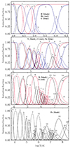 |
Fig. 1. Ionisation fractions of the elements included in our microphysics module under CIE conditions, obtained by integrating until equilibrium is obtained. The first panel depicts the ionisation levels of H (black), He (red), and C (blue); the second panel the ionisation levels of N (black), O (red), and Ne (blue); the third panel the ionisation levels of Si (black) and S (red); and the fourth panel the ionisation levels of Fe (black). |
Mass fractions for Solar abundances (Asplund et al. 2009) and for the wind of a WR star of type WC9 (from Eatson et al. 2022a).
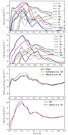 |
Fig. 2. Radiative cooling rates under CIE conditions obtained with our new microphysics module, including elemental contributions Lκ (scaled by (mH/ρ)2 in the first, second, and fourth panels, and by (nenH)−1 in the third panel, respectively) and net cooling function for Solar and WC abundances. Top: elemental contribution of the cooling curve for solar abundances, as specified in Table 2. The black solid line represents the net cooling curve. Second: elemental contribution of the cooling curve for WC abundances, as indicated in Table 2. The blue solid line represents the net cooling curve. Third: comparison of the net cooling curves for solar abundances with those derived by Sutherland & Dopita (1993) and Wiersma et al. (2009). Bottom: net cooling curves for WC abundances compared with the cooling function obtained by Eatson et al. (2022a). |
2.3. Radiative cooling
Cooling rates Λκ, i(ne, T) per electron, per ion of the species κ with charge i are calculated using the CHIANTIPY package v0.10.0 (Del Zanna et al. 2021; Young et al. 2003). The radiative cooling calculation in CHIANTIPY accounts for the radiative loss resulting from the line-emissions of all spectral lines of the specific ion as a function of temperature and electron density (Young et al. 2003; Dere et al. 2009; Del Zanna et al. 2015). In addition, bremsstrahlung emission is taken into account using the expression given in Rybicki & Lightman (1986) with the Gaunt factor calculated using the method of Karzas & Latter (1961). Furthermore, it includes two-photon emission of hydrogen (Parpia & Johnson 1982) and helium (Drake 1986) isoelectronic sequence ions with the spectral distribution function taken from Goldman & Drake (1981) for hydrogen isoelectronic ions and Drake et al. (1969) for helium isoelectronic ions, respectively.
The cooling rates, Λκ, i(ne, T), have been calculated and tabulated on an ion-by-ion basis in NEMO, without assuming ionisation equilibrium and for arbitrary abundances. These cooling rates are valid from 10 K to 109 K and electron densities ranging from 1 cm−3 to 106 cm−3. To validate our implementation, we use the ion and electron number density under CIE conditions for nH = 1 cm−3 and calculate the energy loss rate Lκ = ne∑inκ, iΛκ, i for each element. The net energy loss rate, Lcool, is obtained by summing over the individual species contributions. The normalized cooling function is shown in Figure 2 as a function of T. The top panel in Figure 2 displays the normalized cooling functions of H, He, C, N, O, Ne, Si, S, and Fe under CIE conditions as a function of temperature, derived using ΛN = (mH/ρ)2Lcool and assuming Solar abundances from Asplund et al. (2009).
The net cooling rate exhibits several temperature peaks. The initial peak at approximately 104 K is primarily caused by Hydrogen Lyα cooling, and there are peaks at 105 K, 4 × 10⁵ K, 5 × 10⁵ K, and 1.5 × 10⁶ K, respectively, attributed to contributions from Carbon, Oxygen, Neon, and Iron. In addition, Iron gives a second peak at 2 × 10⁷ K. Other elements also contribute to cooling, with Helium peaking at 4.9 × 10⁵ K, Nitrogen at 5.1 × 10⁴ K, and Silicon with two peaks at 6.3 × 10⁴ and 1.2 × 10⁶ K, respectively. Sulphur also gives two peaks, at 1.5 × 10⁵ and 1.6 × 10⁶ K, respectively. At higher temperatures, the cooling is dominated by thermal bremsstrahlung from fully ionised species.
The second panel of Figure 2 illustrates the cooling function for abundances appropriate for a WR star of type WC9, normalized using the prefactor (mH/ρ)2. The mass fractions of H, He, C, N, and O are obtained from the study by Eatson et al. (2022a), while Solar abundances are adopted for the remaining elements, as given in the last column of Table 2. Compared to the previous case of CIE with solar abundances, the net cooling rate for the WC9 abundance exhibits fewer peaks, with the primary peak occurring at around 105 K due to carbon, followed by a second peak at 2.5 × 10⁵ K due to oxygen and a third peak at 1.2 × 10⁶ K due to carbon again.
The third panel of Figure 2 presents a comparison of the derived CIE cooling function for solar abundances with the seminal works of Sutherland & Dopita (1993) and Wiersma et al. (2009), with all cooling functions normalized by the prefactor (nenH)−1 to maintain consistency. For this calculation we used the Case A recombination coefficients for H and He, to be consistent with the optically-thin assumption of previous work, although for most computations in this paper we used Case B by default (see Sect. 2.4). Our results show a close correspondence with Wiersma et al. (2009) over the full temperature range, while for log(T/K) > 6.0 they also converge with the results of Sutherland & Dopita (1993). Overall, the deviations between our findings and those of Wiersma et al. (2009) are notably smaller than the discrepancies observed with Sutherland & Dopita (1993). These differences can be attributed to variations in elemental abundances and the specific atomic rates adopted in each study.
Similarly, in the bottom panel, we compare our cooling function for WC9 abundances with that of Eatson et al. (2022a), adopting the same abundances used in their study. The comparison with the solar cooling curves in the previous panel of Figure 2 reveals that the cooling rate for WC9 abundances is substantially larger than that for solar abundances at some temperatures. Specifically, the cooling rate is approximately two orders of magnitude greater around 105 K and remains higher for T > 1.5 × 10⁴ K. However, in the temperature range 104 < T < 1.5 × 10⁴ K, the cooling for solar abundances is higher, due to neutral H cooling. There are some differences between our result and that of Eatson et al. (2022a), which we suspect are related to different atomic data and approximations made in the CHIANTI database and the MEKAL model used by Eatson et al. (2022a). These differences are documented and explored in Štofanová et al. (2021), where their fig. 3 shows that the largest differences are at temperatures around 0.01 keV (≈105 K).
2.4. Photoionisation implementation
As discussed above, we employ a variant of the C2-ray method (Mellema et al. 2006) described by Mackey (2012) for photon-conserving radiative transfer and calculation of photoionisation rates, using the method of short characteristics (e.g. Raga et al. 1999; Lim & Mellema 2003) for ray-tracing. In this update, we have extended the method to include several chemical species and multiple frequency bins for the radiation. In this scheme, the photoionisation rate within a grid cell for the species (κ, i) to species (κ, i + 1) is expressed as
where τν is the optical depth from the source to the front edge of the cell, Δτνκ, i represents the optical depth along a ray within the cell for the species (κ, i), Vshell has the same meaning as in Mellema et al. (2006), and Lν is the spectral luminosity of the radiation source.
We further replace the frequency integration by Riemann summation over energy bins making the above equation
where the index j iterates over the energy bins, L* represents the total luminosity of the star, and Fj is the fraction of the total photon energy density in bin j. The average optical depth in each energy bin, denoted by  , is computed by the ray-tracing module by summing cell optical depths along the ray. The cell optical depth for the species (κ, i) is given by
with nκ, i representing the number density of the photo-species (κ, i) in the cell, and Δr the cell depth. Species with ionisation threshold energies lower than the maximum energy of the energy bins are treated as photo-species. The mean cross-section  for the species (κ, i) in energy bin j is determined following Mackey (2012) using the expression

where  is the mean energy of bin j. The integration is evaluated using the composite Simpson’s 3/8 rule over the range of energy bin j. The photoionisation cross sections, σκ, i(E), in the above equation are calculated using the analytic fit formula presented in Verner et al. (1996).
Note that dust grains may be an important source of opacity in far UV and EUV, and our exclusion of dust physics means that we may underestimate the absorption of ionising radiation in regions where dust is present. The winds of hot stars are dust free except where dust forms in colliding winds of some WC binary systems, and so our model remains applicable in stellar-wind bubbles but becomes less accurate once a significant column density of dusty ISM or CSM has been traversed.
Photo heating Qphoto is calculated in a similar manner and is given by
The summation is performed over photo-species, and the individual contributions Qκ, i are calculated following Mellema et al. (2006) using the equation
The binned spectral energy distribution, Fj in the above expressions are pre-calculated for ATLAS stellar atmosphere models (Castelli & Kurucz 2003) and Potsdam WR models (Hamann & Gräfener 2004; Sander et al. 2012; Todt et al. 2015). The ATLAS9 model library encompasses a wide range of elemental abundances, represented by [M/H], spanning from solar metallicity (0.0) to metal-poor conditions (−2.5). Furthermore, it covers a broad gravity range from log g = 0.0 to +5.0, with increments of +0.5. The effective temperature grid ranges from 3500 K to 50 000 K, but it is not evenly spaced. These models are designed to provide spectral information spanning from 1.6 × 10⁶ Å to 90.9 Å, with varying wavelength intervals. The Potsdam WR Models gives spectral profiles of WR stars of the nitrogen subclass (WN). They offer two distinct varieties: hydrogen-free models (WNE) and models with a specified mass fraction of hydrogen (WNL). Moreover, these models cater to diverse metallicities, corresponding to the iron-group and total CNO mass fractions, which align with the metallicities of the Galaxy, the Large Magellanic Cloud (LMC), or the Small Magellanic Cloud (SMC), respectively.
For calculations in this paper the radiation field was divided into 15 energy bins in the range hν ∈ [7.9, 77.0] eV. The boundaries of the energy bins were chosen to coincide with the most important ionisation energies for the ions considered, and are quoted in Table 5. The ray-tracing module in PION only tracks direct radiation from sources to the point it is absorbed, and does not track scattered or re-emitted radiation. Instead we assume the On-the-Spot (OTS) approximation, where recombinations to the ground state of H emit a photon that is assumed to locally re-ionise another H atom. To achieve agreement between PION and CLOUDY for the radius of the He+ and H+ ionised zones (see Sect. 3.4), it was necessary to correctly account for re-ionisations of H and He by recombinations of He2+ and He+. We followed the method of Friedrich et al. (2012) to correctly allocate recombination photons to the ionisation of H and He. The algorithm will be considerably more complicated to implement for arbitrary elemental abundances; this is deferred to future work. To calculate the recombinations into different energy levels the case A recombination rate is augmented with case B recombination rates for H+, He+ and He2+, taking the fitting functions from Hui & Gnedin (1997).
2.5. Charge-exchange
Charge exchange can be an important process in partially ionised zones where H (or He) is mostly neutral but other species may be ionised (for example, O). We consider recombination reactions with H and He of the type:

where q is set from 1 to 4, A is H or He, and Bq is the recombining ion with charge q. The reverse ionisation reactions involve H+ and He+ donating an electron to ionise a heavier ion:

The energy defect ΔE in the above equation can be either positive or negative, depending on the reaction.
We base our calculations on the parameters provided by Kingdon & Ferland (1996) for the analytic fit formula of Arnaud & Rothenflug (1985). This formula is used to determine the rate coefficient for recombination charge-exchange reactions with H, as listed in Table A.1. The corresponding rate coefficients for reverse (ionisation) reactions are listed in Table A.2 and are related to the forward rates by the principle of detailed balance, expressing the ionisation rate coefficients as a product of the fitting function and the Boltzmann factor exp(−ΔE/kT). For He charge-transfer recombination reactions, also shown in Table A.1, we apply the fitting formula and parameters from Arnaud & Rothenflug (1985). We generate a lookup table for the ionisation and recombination reaction rate coefficients  , pertaining to the reactant species (κ, i) and (s, q) as a function of temperature.
The source term due to charge exchange can be explicitly expressed as:
The first term in this expression represents the contribution of all reactions leading to the recombination of species transitioning from (κ, i + 1)→(κ, i). The last term accounts for the ionisation of species transitioning from (κ, i − 1)→(κ, i). The second term addresses both recombination and ionisation, representing the transitions of species from (κ, i)→(κ, i − 1) and (κ, i)→(κ, i + 1), respectively. These transitions, driven by charge transfer, can heat the system as shown in Tables A.1 and A.2 which indicate that most reactions are exothermic. The heating due to charge transfer (Qcx) is given by:
where  is the energy gain from the reaction involving the reactant species (κ, i) and (s, q).
To confirm the precision of calculation, we conduct collisional ionisation equilibrium simulations using the same initial conditions as our previous one reported in Sect. 2.2, but with charge exchange reactions enabled and q set to 4. Figure 3 illustrates the equilibrium ionisation balance for N, O, Ne, and Si, comparing scenarios with and without charge exchange reactions over the temperature range of 104 − 105 K. The ionisation profiles exhibit significant differences, aligning well with the results from the literature (Gu et al. 2022; Arnaud & Rothenflug 1985). The slight variations in the profiles are due to minor changes in the rate coefficient values.
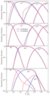 |
Fig. 3. Comparison of CIE balance for N, O, Ne, and Si incorporating and omitting charge exchange (CX) reactions with H and He. Solid curves represent ionisation fractions with charge exchange calculations, while dashed curves represent ionisation fractions without charge exchange reactions. |
3. Results
Here we examine a series of 1D calculations using NEMO for adiabatic shocks, radiative shocks, and H II regions that can be compared with solutions from the literature. We first examine shock models similar to Model E from Raymond (1979) within a 1D Cartesian framework, specifically employing slab symmetry. The setup features a uniform inflow from the positive x-boundary and a reflecting condition at the negative x-boundary. Table 3 outlines the simulation domain alongside the uniform initial density ρ0, velocity vx, 0, temperature T0, and magnetic field By, 0. The other velocity and magnetic field components are zero in the initial conditions and remain zero due to the symmetry.
Model E in Raymond (1979) utilizes abundance set A, which is based on the cosmic abundances from Allen (1973). We adopt the same abundance set, with the exception of Mg and Ca. Consequently, we track 99 chemical species across the four shock tests detailed in the following subsections. These tests aim to assess the accuracy of our calculations concerning the distinct flow properties and physical processes presented in Table 3.
The H II region tests are based on the HII40 Lexington benchmark test (Ferland 1995), including multi-frequency ionising radiation, all ionisation or recombination and heating or cooling processes, but no hydrodynamics.
3.1. Adiabatic shock test 1
Shock Test 1a is an adiabatic shock with Mach number of about 10. Figure 4 illustrates the flow structure of the shock, which is formed by the inflowing neutral gas travelling at a speed of 100 km s−1 with a pre-shock particle number density n of 10 cm−3. The shock velocity, vsh = 133 km s−1, is larger than 100 km s−1 because it reflects off the negative boundary and propagates upstream at velocity (vsh/4) km s−1 by conservation of mass in the (adiabatic) downstream layer. The Rankine-Hugoniot jump condition compresses the gas by a factor of 4 and predicts a post-shock temperature of
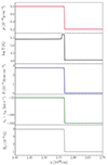 |
Fig. 4. Flow quantities of an adiabatic shock generated by gas flowing at a velocity of 100 km s−1. The simulation employs 10 240 grid cells and not all of the domain is shown. |
where μ is the mean mass per particle in unit of the hydrogen atom mass, mH, and we assume an adiabatic index of γ = 5/3 for the gas equation of state. For vsh = 133 km s−1 this results in post-shock temperature of T = 4.9 × 10⁵ K.
The kinetic energy of the gas upstream of the shock is converted into thermal energy as it transitions through the shock front, resulting in an increase in the temperature of the gas downstream, and consequently collisional ionisation.
In the post-shock relaxation layer, this thermal energy ionises the gas by removing ionising potential energy from the gas, as given by the expression
where Iκ, i denote the ionisation potential of the ion of the species κ and charge i. Due to the rapid ionisation, we observe an drop in the temperature to 2.5 × 10⁵ K immediately after the shock. This is almost entirely due to H ionisation because it is the most abundant element. In this way the neutral state of the pre-shock gas significantly influences the post-shock temperature far downstream from the shock.
Figure 5 depicts the ionisation fraction profiles across the shock front region for a gas composed of neutral atoms of H, He, C, N, O, Ne, Si, S, and Fe. In this context, where radiative losses are absent, the gas tends towards equilibrium to the left, stabilizing at a temperature of 2.51 × 10⁵ K. At this equilibrium temperature, hydrogen and helium demonstrate nearly complete ionisation, with ionisation fractions of 0.999 for H1+ and 0.998 for He2+. Among other elements, notable ionisation states include C4+ at 0.989, N4+ at 0.104, N5+ at 0.866, O3+ at 0.224, O4+ at 0.533, O5+ at 0.144, Ne3+ at 0.214, Ne4+ at 0.664, Ne5+ at 0.111, Si4+ at 0.914, S6+ at 0.904, Fe6+ at 0.129, and Fe7+ at 0.857. These values closely match the ionisation fraction obtained in the CIE test depicted in Fig. 1 for a temperature of 2.51 × 10⁵ K. The gas achieves the ionisation state over a finite timescale, determined by the specific recombination and ionisation rates of the species at the given temperature.
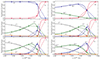 |
Fig. 5. Spatial profiles of ion fractions for H, He, C, N, O, and Ne across the shock front for shock test 1, comparing the low (dashed lines) and high (solid lines) resolution simulations. The flow moves from right to left, with the shock positioned at the plot’s right-hand boundary. The plot depicts only the downstream region. |
Figure 5 compares the ionisation profiles of H, He, C, N, O, Ne, Si, S, and Fe across the shock front for both low (1024 grid points, Δx = 4.8828 × 1013 cm) and high resolution (10240 grid points, Δx = 4.8828 × 1012 cm) simulations (shock test 1b) for the same domain size of 5.0 × 1016 cm. Despite the substantial resolution discrepancy, these simulations exhibit noteworthy agreement, particularly away from the shock. However, this agreement diminishes in the immediate vicinity of the shock, primarily due to the rapid temperature variation across the shock. As the gas swiftly ionises to a state consistent with the local temperature, facilitated by the small ionisation timescale, significant spatial changes occur near the shock front, necessitating a higher resolution grid to accurately capture these nuances. Yet, this requirement pertains specifically to the immediate shock region, with overall agreement between low and high resolution simulations remaining relatively robust.
3.2. Non-adiabatic shock tests 2 and 3
As an extension of the preceding planar shock test, we conduct the shock tests under non-adiabatic conditions for higher inflow velocities with cooling turned on and no radiation sources. The flow structure of a neutral pre-shock gas of density 5.0935 × 10⁻²³ g cm−3 intersecting the shock front at a velocity of 1000 km s−1 are illustrated in Fig. 6. The two panels display temperature and density profiles at two distinct time points. Initially, at t1 = 1.2945 × 10⁴ years, the post-shock gas remains uncooled, maintaining a temperature of T ∼ 1.5 × 10⁷ K, determined by the Rankine–Hugoniot jump conditions, because the post-shock cooling timescale is longer than the simulation has been running for. Later, at t2 = 1.2799 × 10⁵ years, the downstream gas, particularly the region farthest from the shock front, undergoes significant cooling, with the temperature dropping to T ∼ 3.0 × 10³ K, as depicted in the bottom panel of Fig. 6.
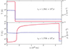 |
Fig. 6. Illustration of the flow structure in pre-shock gas interacting with the shock front. The top panel exhibits temperature (red-solid curve) and density (blue-dashed curve) profiles at t1 = 1.2945 × 10⁴ years, while the bottom panel presents the same at a later time, t = 1.2799 × 10⁵ years, highlighting the interplay between Chianti cooling data and gas dynamics. |
The top (H and He) and bottom (C) panels of the Fig. 7 show the non-equilibrium ionisation structure of the post-shock gas as it undergoes cooling. Initially, H, He, and C exist in a fully ionised state immediately behind the shock front. As the downstream gas gradually cools from an initial temperature of T ∼ 1.5 × 10⁷ K to T ∼ 3.0 × 10³ K, one can observe the transition in the ionisation state of the gas, progressing from its most ionised state to a neutral state (from right to left).
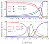 |
Fig. 7. Ionisation fractions of H, He, and C within the cooling region of non-adiabatic shock test 2, revealing non-equilibrium dynamics of chemical species at later time, t = 1.2799 × 10⁵ years. |
Figure 8 presents a comparison of the ionisation profiles of Si for two higher inflow velocities: 1000 km s−1 in the top panel (shock test 3a) and 3000 km s−1 in the bottom panel (shock test 3b). Here the post-shock temperature is sufficiently high that the cooling length-scale is larger than the simulation domain and the shock behaves adiabatically. However, the ionisation profiles in the immediate vicinity of the shock front show a clear dependence on the inflow velocity.
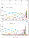 |
Fig. 8. Spatial profiles of ion fractions for different ionisation levels of Si across the shock front in non-adiabatic flows at velocities of 1000 km s−1 (top panel) and 3000 km s−1 (bottom panel). |
The higher post-shock temperature associated with larger inflow velocity of 3000 km s−1 results in increased ionisation rates, subsequently leading to shorter ionisation timescales. This phenomenon, as discussed in the previous section, implies that smaller ionisation levels of chemical species exhibit reduced spatial extents. To resolve the spatial profile of ionisation fractions for each ionisation state of the elements within the post-shock ionisation layer, a fine spatial resolution is imperative. Consequently, the simulations were conducted with 10 240 grid cells to ensure precise spatial delineation.
The ionisation process unfolds progressively from right to left, initiating from the shock front. This sequential progression occurs due to the finite ionisation time scale associated with each ionisation state. Behind the shock, the temperature rises sufficiently to enable ionisation across multiple levels of Si ions. The significance of higher ionisation states manifests only at a specific spatial distance from the shock front, owing to the time required for successive ionisation processes, contingent upon the gas temperature in that region being high enough to facilitate such ionisation. Consequently, the emission spectra observed immediately behind the shock primarily reflect the presence of lower ionisation states within the gas chemical species. Conversely, emission from highly ionised gas is observable away from the shock front.
3.3. Charge transfer non-adiabatic shock test 4
In this section, we extend the previous non-adiabatic shock model to incorporate charge exchange with q = 4 (see Sect. 2.5), tracing all ionisation levels of H, He, C, N, O, Ne, Si, S, and Fe. This integration includes all the reactions listed in Tables A.1 and A.2. As in previous cases, we assume a neutral pre-shock gas, but now with a slower inflow velocity of 120 km s−1. This adjustment results in a steady-state shock similar to the one presented in Butler & Raymond (1980).
Figure 9 compares the temperature distribution and ionisation states of O behind the shock front with and without charge exchange reactions after ∼5 × 10² yrs. The minimal variation in the temperature profile indicates that heating due to the charge exchange reactions listed in Tables A.1 and A.2 is insignificant. However, there is a notable impact on the ionisation of the gas, as shown by the ionisation states of O in the bottom panel of Figure 9.
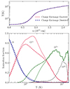 |
Fig. 9. Temperature and ionisation profiles of the shocked gas with and without charge transfer processes. The top panel shows temperature as a function of position, with the shock off the grid to the right, and the flow from right to left. The temperature profile with and without charge-exchange is almost identical. The bottom panel shows the ionisation fractions of oxygen, emphasizing the significance of charge transfer reactions for the oxygen ionisation state, especially below 6 × 10³ K. |
When the temperature decreases to 105 K, the reaction rate for O2+ + H → O+ + H+ becomes significant, with a value around ∼10−9 cm3 s−1, considerably higher than the corresponding radiative recombination rate, although at this high temperature the electron abundance is much larger than the neutral H abundance, reducing the importance of charge exchange. At temperature 30 000 K, the fractional abundance of neutral hydrogen increases enough to allow the charge-exchange reaction to become the dominant process. At 20 000 K, the O+/O2+ ratio is significantly larger compared to the case when charge exchange reactions are omitted. Below 10 000 K, the reaction O+ + H → O + H+ gains importance, maintaining a rate of about ∼10−9 cm3 s−1. The reverse ionisation reaction O + H+ → O+ + H also proceeds rapidly, with a rate ∼9 × 10⁻¹⁰ cm3 s−1. These competing reactions ensure ionisation balance remains largely unaffected by charge transfer.
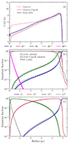 |
Fig. 10. Photoionisation equilibrium calculation for the temperature and ionisation state of a static H II region for a H number density nH = 10 cm−3: (a) gas temperature vs. radius for 3 different calculations: dotted-red line obtained with CLOUDY, dashed-red line CLOUDY with the Case-B setting and solid-blue line shows the result with PION using the On-the-Spot approximation (see text for details); (b) ionisation state of H and He as a function of radius: solid lines are results obtained with PION, dotted lines with CLOUDY and dashed lines CLOUDY+CaseB; and (c) as (b) but showing ionisation state of O as a function of radius. |
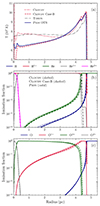 |
Fig. 11. Photoionisation equilibrium calculation for the temperature and ionisation state of a static H II region for a H number density nH = 100 cm−3 (The Lexington HII40 benchmark test): panels (a), (b), and (c) as for Fig. 10 except that panel (a) also includes the result from TORUS. |
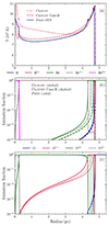 |
Fig. 12. Photoionisation equilibrium calculation for the temperature and ionisation state of a static H II region for a H number density nH = 1000 cm−3: panels (a), (b), and (c) as for Fig. 10. |
3.4. HII region test
To validate the photo-ionisation subroutine, we conducted an HII region simulation following the HII40 Lexington benchmark test (Ferland 1995). The simulation utilized a one-dimensional, uniform grid with spherical symmetry, comprising 512 grid zones and covered a radial domain extending from the origin to r = 1.8 × 1019 cm. At the centre is a blackbody radiation source with an effective surface temperature of 40 000 K, irradiating an initially neutral, cold and uniform ISM. Hydrodynamics is switched off, and the system is integrated until photoionisation equilibrium is achieved. Three calculations were run, with parameters as indicated in Table 4: Test 2 is the HII40 Lexington benchmark model (Ferland 1995) (note that the elemental abundances are quoted in terms of mass fraction rather than the more typical number fraction relative to H) and Tests 1 and 3 are variants with lower and higher gas density, respectively. The ionising photon output of the source was decreased or increased for tests 1 and 3 to give the same Strömgren radius as for Test 2 (test 3 obviously has an unreasonably large luminosity for a stellar source and is run only for comparison with the other two tests). We used 15 energy bins for the radiation field, listed in Table 5. In Appendix B the dependence of our results on the energy binning is quantified.
Simulation parameters used for the H II region test with the HII40 Lexington benchmark model (Ferland 1995; Ercolano et al. 2003; Haworth & Harries 2012).
Energy bins for the radiation field for photoionisation calculations, chosen to line up with ionisation thresholds of the modelled ions, as much as possible.
We used CLOUDY version C23.01 (Chatzikos et al. 2023) to make a comparison with our results. For Test 2 we also compared the results with published data from TORUS (Haworth & Harries 2012). After finding differences between the results from PION and CLOUDY for the temperature structure of the H II region, we also ran CLOUDY with the CaseB setting, which effectively switches off transport of recombination radiation beyond the Lyman limit by setting the local optical depth for this radiation to very large values. This imposes the well-known OTS approximation (see Sect. 2.4), where recombinations to the ground state are assumed to result in local ionisations. This assumption is not correct for some gas densities, but it more closely mimics the radiative transfer in PION, which makes the OTS approximation.
Results for Tests 1, 2 and 3 are shown in Figs. 10, 11 and 12, respectively. In each case the top panel shows gas temperature as a function of radius for the converged final state; the middle panel shows ionisation fractions of H and He; and the bottom panel ionisation fractions of ions of O. The main result shown here is the close agreement between PION and CLOUDY in ‘Case B’ mode for the temperature and ionisation fraction as a function of radius, especially for tests 1 and 2. The location of the He2+, He+ and H+ ionisation fronts are in good agreement; only for the high-density test 3 is the location of the He+ ionisation front offset significantly. The ionisation state of O follows closely that of He and H, and so the two codes show good agreement for tests 1 and 2, but diverge somewhat for test 3 at the O2+ → O+ transition. For test 3 there is also a significant difference in the location of the He+ ionisation front between CLOUDY runs with and without Case B, and so we suspect this is related to the simplified radiative transfer treatment in PION.
The reason for the divergent temperature structure between PION and the standard settings of CLOUDY appears to be in the transport of the diffuse radiation field generated by recombinations. PION uses a simple ray-tracer to transport radiation directly from the source until it is absorbed, without scattering, and assumes any re-emitted or scattered radiation is re-absorbed locally (the OTS approximation). The interior of the H II region is, however, optically thin to ionising radiation, and so this assumption breaks down towards the origin. The good agreement with CLOUDY in ‘Case B’ mode lends support to this interpretation. A more accurate radiative transfer scheme is beyond the scope of this work, but could potentially be achieved by coupling the multi-ion module to a radiative transfer scheme that treats every cell as a source, example, TREERAY (Wünsch et al. 2021).
There is a noticeable feature in the extension of a low level of He+ ionisation beyond the ionisation front in PION runs, and in CLOUDY runs for test 3. This is not related to charge exchange because the feature persists when this process is switched off. Despite some effort we were unable to track down the source of this feature; we suspect it is related to radiative transfer of the hard photons and possibly sub-optimal arrangement of the energy bins. Further investigation is deferred to a future work where we will implement a generalised OTS approximation including recombination radiation from, and ionisations of, all ions in the network.
4. 1D example application: wind-wind interaction
We conducted a one-dimensional, spherically symmetric radiation-hydrodynamics simulation to investigate the interaction between the stellar winds of a red supergiant (RSG) star that evolves to become a WR star when it loses its H-rich envelope. This simulation highlights the versatility of our module, effectively handling the distinctly different elemental abundances of the two winds and integrating all relevant physical processes, including photo-ionisation, collisional ionisation, recombination, and charge exchange reactions.
For this calculation we track 7 elements (H, He, C, N, O, Ne, Si) and their ionisation states by solving 51 ordinary differential equations and 7 constraint equations. The simulation used a spherically symmetric, nested grid with five levels, each containing 256 grid cells, with the coarsest level covering a radial domain of 3.7028 × 1019 cm. Each refined grid level, centred at the origin, has double the spatial resolution of the previous one and half of the domain size, with the same number of zones. The details of the 1D nested grid are described in Fichtner et al. (2024).
The parameters defining both the stellar and circumstellar medium (CSM) are detailed in Table 6. We model the CSM as being generated by the freely expanding stellar wind of a RSG with a terminal velocity, v∞ = 25 km s−1 and mass-loss rate Ṁ = 2.0 × 10⁻⁵ M⊙ yr−1. The density is given by the conservation of mass:
Thus, the CSM follows an inverse-square density distribution, and the elemental abundances are solar values from Asplund et al. (2009) (see Table 6).
Further, the WR wind and CSM are photo-ionised by a central WR star of the carbon subclass (WC), characterized by a mass of 11.6 M⊙, an effective surface temperature of 105 K, a stellar radius of 2.102 R⊙, and a total luminosity of 1.524 × 1039 erg s−1 (3.952 × 10⁵ L⊙). We adopt the Potsdam WR model with Galactic WC abundances for the spectral energy distribution of the central star, which is divided into Nb = 15 energy bins spanning the energy range of 7.64 to 77.0 eV, as detailed in Table 5. The WR stellar wind is injected from the stellar surface with a mass-loss rate of Ṁ = 3.0 × 10⁻⁵ M⊙ yr−1, and a wind terminal velocity of v∞ = 1500 km s−1 with chemical composition given in Table 6.
Parameters for 1D MHD Simulation of Wind-Wind Interaction: Ionising Source, Stellar Wind, and CSM.
Figure 13 displays the flow quantities and ionisation profiles of H, He, C, N, and O for the spherically symmetric interacting winds at t = 3.5007 × 10⁴ yr. The top panel shows the typical characteristics of a stellar wind bubble formed by the strong ram pressure of the central WR star wind, which sweeps up the slower wind from the RSG. A key chemical feature distinguishing the WR wind from the RSG wind is the absence of H and N, demonstrated in the top panel by nH. The rapidly increasing nH at r ≈ 9 pc marks the contact discontinuity between WR wind and RSG wind, mirrored by a rapid decrease in T with r. The finite width of this feature is a result of numerical diffusion in this relatively low-resolution simulation.
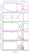 |
Fig. 13. Snapshot from 1D simulation of wind-wind interaction from a WR wind expanding into a pre-existing RSG wind from a previous evolutionary phase. The top panel displays the flow quantities, and the subsequent panels show the ionisation profiles of H, He, C, N, and O, all at a time 35 kyr after the initiation of the WR wind. |
4.1. Ionisation profile
The stellar wind region is characterized by mechanical motion, with thermal energy remaining relatively low at around the minimum temperature in the simulation. ionisation in this area is entirely driven by photoionisation. Helium is almost entirely ionised, with over 63% existing as He2+ and the rest as He1+. Carbon is primarily found as C3+, making up about 95% of all carbon in the stellar wind. Hydrogen is extremely scarce, with an abundance of only 10−8 in the stellar winds of WC stars. Furthermore, the prevalent ionisation states of other elements include N3+ and O2+.
The expansion of the wind-wind interaction follows the constant velocity evolution described by Koo & McKee (1992). The wind-wind interaction region is bounded by a forward shock expanding into the RSG wind and a reverse shock propagating into the WR wind. The reverse shock is adiabatic, whereas the forward shock is partially radiative. This region is of particular interest due to its large temperature range, spanning approximately 2 × 10⁴ K to 8.8 × 10⁷ K. The regions of shocked RSG wind and shocked WR wind are separated by a contact discontinuity, where the temperature sharply decreases from around 2 × 10⁷ K to 2.7 × 10⁵ K within a narrow region of width about 0.5 pc.
In the shocked WR wind region, temperatures range from roughly 8.8 × 10⁷ K to 2 × 10⁷ K over a span of about 2.3 pc. This area is dominated by highly ionised species, namely He2+, C4+, N4+, N5+, O3+, O4+, O5+, and O6+. In this region, collisional ionisation overshadows photoionisation, indicating that the ionisation state of the gas is more significantly influenced by wind velocities and its chemical composition than by ionising photons from the central star. In the shock reference frame, protons moving at 1500 km s−1 have kinetic energy of nearly 12 keV, much larger than the maximum photon energy considered for photoionisation (77 eV), and so the ionisation state is determined by collisional processes. Figure 13 shows that the ionisation timescale in this rarefied plasma is long enough that it is spatially resolved in the shocked WR wind. We see successively higher-ionised states of C,N,O (and other elements not shown) up to the location of the contact discontinuity, with an ionisation length-scale of about a parsec, and the equilibrium ionisation states are not reached.
Conversely, the composition and temperature profile of the shell of the swept-up RSG wind are distinct from the shocked WR wind region. Although the temperature in this region remains high enough for collisional ionisation to dominate, the prevalent ions are different. The outer shock is partially radiative and expands at about 265 km s−1 into the RSG wind, at almost constant velocity according to Koo & McKee (1992). The relative velocity of the shock to the RSG wind is therefore 240 km s−1, and post-shock temperature of ∼0.3 keV. The density in the shocked RSG wind is much larger than in the shocked WR wind, and so the ionisation timescale (and length-scale) is much shorter. This region exhibits a large fraction of H1+ and He2+, with C4+, N5+, and O6+, especially around the contact discontinuity.
Furthermore, the ionisation of He2+ drops immediately at the forward shock front. This phenomenon is attributed to the Strömgren sphere associated with He2+ being located within the shocked wind region.
Beyond the forward shock the temperature is approximately 20 000 K, with the density of the RSG wind diminishing like r−2. A rough calculation shows that the Strömgren radius is on the order of kpc. This region is predominantly characterized by photoionisation, with the high temperature resulting from photo-heating. At a distance of 12 pc, the dominant ionised species are H1+, He1+, C3+, N3+, and O2+. The RSG wind has been photo-ionised and photo-heated to above the equilibrium temperature, but the cooling time is longer than the simulation runtime for this low-density outer-wind region.
4.2. Line luminosities
The line radiation mechanism plays a key role in energy loss from hot plasma environments. The high-temperature regions resulting from wind-wind interactions provide an excellent context for analysing the relationship between line emission, elemental abundances, and ionisation fractions. Here, we calculated the time-dependent line luminosities for selected transitions of oxygen and nitrogen, as illustrated in Figure 14. These luminosities were computed at each time step using the CHIANTI atomic database through the CHIANTIPY package v0.10.0 (Del Zanna et al. 2021; Young et al. 2003). The wind-wind simulations provide ion density and temperature for each spherical cell, allowing us to compute the spectral line emissivity based on local cell temperature and to integrate it using the equation:
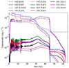 |
Fig. 14. Time evolution of luminosity for selected oxygen and nitrogen emission lines for the 1D wind-wind simulation in Sect. 4, calculated as described in Sect. 4.2. The forward shock leaves the domain at around 45 kyr, and the associated sharp drop in some line luminosities is therefore artificial. |
to derive the line luminosity at a specific time, where ϵs, q(λ, ne, T) represents the emissivity at wavelength λ and plasma electron density ne and temperature T, with units of erg s−1 sr−1 ion .
.
Figure 14 shows the evolution of the luminosity of a range of strong nebular lines for the duration of the simulation. We observe distinct behaviours among different spectral lines; however, lines with similar characteristics can be grouped together. For instance, the forbidden line doublet O IIIλλ5007, 4959, which are prominent nebular oxygen lines, exhibit similar trends. The luminosity of these lines continues to decrease as the nebula expands. This decline is primarily due to the decreasing mass density of the photo-ionised OIII ion, which is prominent only in the unshocked WR and RSG wind regions. As the thin WR wind expands, displacing the denser RSG wind, the density of O III decreases accordingly. The abrupt drop in luminosity around t ∼ 47 kyr is attributed to the dense shocked shell leaving the simulation domain, leading to a sharp reduction in the total mass density.
The second group of lines, which exhibit similar trends, includes NIVλλ3478, 3485, OIVλλ3403, 3413, and OVIλλ3811, 3834. These lines are less luminous, with luminosities ranging from 1028 to 1031 erg s−1. While NIV is a dominant ion in the expanding WR and RSG wind regions, and OIV and OVI are confined to the shocked regions, they display comparable behaviour. This similarity arises from the fact that NIV also forms in the cooling shocked shell and has an ionisation fraction similar to that of OIV and OVI in this high-density region. This correlation suggests that the luminosity of these lines is primarily dictated by the density of the shocked shell. The WR wind has a very low overall N abundance and so contributes little to the N IV emissivity.
The most intriguing lines are OVIλλ1032, 1038, whose luminosity steadily increases up to 47 kyr and becomes the strongest of the lines that we calculate. This gradual rise is attributed to the increasing mass of the shocked shell as the WR wind sweeps up the RSG wind material. When the shocked shell exits the simulation domain, there is an abrupt decline in luminosity. Interestingly, after 47 kyr, the log luminosity follows a linear trend until 63 kyr, driven by the contribution of OVI in the shocked WR wind region. This behaviour indicates that the mass density associated with OVI decreases exponentially over time within the simulation domain. Lastly, the OIVλ258933 line, one of the prominent oxygen lines, exhibits a trend similar to that of OIIIλλ5007, 4959. However, after around t ∼ 47 kyr, its luminosity stabilizes, remaining constant. This behaviour is attributed to the unchanging density profile of OIV ions in the freely expanding wind, which is sustained by photoionisation from the central star.
The line luminosity of some lines calculated and plotted in Fig. 14 show strong oscillations particularly at early times in the evolution of the nebula. This arises because we do not spatially resolve the post-shock ionisation length of the forward shock at early times, and the emission from these lines is often dominated by only one or two cells in the post-shock region. Depending on the position of the shock within a cell, the emission calculated for intermediate ionisation stages in the post-shock cell may vary substantially. One can also see when the swept-up shell crosses grid-refinement boundaries at t ≈ 3, 6, 12, 24 kyr from small step changes in the luminosity of particularly O III lines. These are related to adjustments in the hydrodynamic structure of the shocks and swept-up shell as they move to a region with larger numerical diffusivity.
4.3. 2D wind-wind interaction
We also perform two-dimensional radiation-hydrodynamics (RHD) simulations to model the interaction between the stellar winds of the RSG and WR stars. These simulations are conducted in cylindrical coordinates, assuming rotational symmetry, using a computational grid in the (R, z) plane. The star is located at the origin, (R, z) = (0, 0), within a rectangular simulation box. The grid has a resolution of 128 × 256 cells at each level, and the coarsest level has a domain R ∈ [0, 3.7028 × 10¹⁹] cm, and z ∈ [ − 3.7028 × 10¹⁹, 3.7028 × 10¹⁹] cm. There are five grid levels, each centred at the origin, with each level having a spatial resolution twice as fine as the preceding coarse grid while maintaining the same number of zones, and with domain 2× smaller in each dimension. The simulation parameters for both the stellar and circumstellar medium (CSM) are the same as those used in the one-dimensional simulations, as detailed in Table 6, except that the wind boundary region (where the wind is injected) is set to 10 grid zones to reduce grid-related artefacts. The simulation required about 104 core-hours to complete, using 64 cores (8 MPI processes and 8 OpenMP threads per process).
Figure 15 shows a snapshot of the gas density and temperature on logarithmic scales, after about 23 kyr of evolution. The nebula evolves with almost spherical symmetry because the central star is able to fully ionise the whole domain very rapidly, so that D-type ionisation fronts (with their associated instabilities, Garcia-Segura & Franco 1996) do not develop. Furthermore the wind termination shock is adiabatic, as seen in the 1D simulation, and the forward shock is also very close to adiabatic; there is a cooler, denser layer near the contact discontinuity but it is expanding faster than it can cool (also seen in 1D). Some grid-related features are visible around the termination shock and contact discontinuity; these arise from the wind injection boundary and become less apparent with higher resolution.
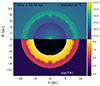 |
Fig. 15. Snapshot from a two-dimensional simulation captures the interaction between the WR wind and the remnant wind from the earlier RSG phase. The image shows the flow quantities 23.36 kyr after the onset of the WR wind, with the star located at the origin. The top panel shows log10 of gas density (g cm−3) according to the colour scale shown, where brighter yellow regions indicate higher density, and darker purples represent lower density. The bottom panel shows log10 of temperature (in K) according to the colour scale displayed beside the plot. |
Figure 16 shows the ion fractions of the main species of oxygen in the domain (there is negligible O0 or O+ present because of the hard radiation field of the WR star). The same features as from the 1D case (Fig. 13) are apparent: the freely expanding wind and the unshocked RSG wind are almost entirely in the form of O2+, successively higher ionisation stages are reached at larger radius in the shocked WR wind, and the shocked RSG wind is primarily O6+. The shocked WR wind never reaches equilibrium ionisation (O8+). Overall the results agree very well with the 1D calculation.
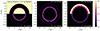 |
Fig. 16. Ionisation profile of O2+ to O7+ ions from a two-dimensional simulation of the interaction between the WR wind and the remnant RSG wind, shown 23.36 kyr after the onset of the WR wind. The panels illustrate the ionisation fraction, YO, i on a linear scale, with white representing a oxygen completely in this ionisation state (YO, i = 1) and black denoting the zero abundance (YO, i = 0). The colour scale is shown at the far right of the plot. |
5. Discussion
5.1. Simulation performance
Here we investigate the impact of chemical tracers on the computational efficiency of MHD simulations. We use a modified version of the Raymond planar shock model E, changed to have an inflow rate of 1000 kms−1 and a transverse magnetic field of 10−6 G. We perform several simulations with sequential addition of tracers, including H, He, C, N, O, Ne, Si, S, and Fe, along with their respective ionisation states for a fixed simulation time of 3.156 × 10⁹ s, using a uniform 1D grid of 256 grid zones and slab symmetry.
Figure 17 shows the wall-time and cell update-speed as a function of the function of number of tracers, Ntracer, for runs with 10 and 15 OpenMP threads. For this test we included only collisional processes excluding charge exchange. The wall-time required is the sum of the microphysics update, the MHD update, and the boundary updates, but the runtime is quickly dominated by the microphysics solver as Ntracer increases. For large Ntracer it looks like the update speed approaches a Ntracer−2 scaling.
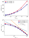 |
Fig. 17. Relation between simulation speed and the number of tracers (elements plus their ions). The upper plot shows the wall-time of a 1D simulation using from one to nine elements, with either 10 or 15 OpenMP threads on 10 or 15 cores. The lower panel shows the same data, calculating the number of cells updated per core per second. This 1D shock calculation did not include photoionisation or charge-exchange reactions (see text for details). |
We also examine how the runtime scales with the number of OpenMP threads, Nthread, in the same shock test, but this time including the charge-exchange reactions with q = 4. The results are shown in Figure 18.
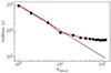 |
Fig. 18. Parallel scaling of the same 1D shock test as Fig. 17 (except that now charge-exchange reactions are included), showing the simulation wall-time as a function of the number of OpenMP threads (and cores) used for the calculation. This is compared with the ideal speedup of Nthread−1 (dashed line). |
The wall-time decreases as Nthread−1 up to 10 OpenMP threads and there is little gain beyond going to 30 threads. This is partly because for 1D tests the MHD and boundary updates are not multi-threaded. Each OpenMP thread operates on a 1D column of cells for MHD, whereas the threads operate on a cell-by-cell basis for the microphysics update.
Overall the code performs as expected and, when running with all 9 elements and 99 tracers, the update speed is about 1000× slower than an MHD calculation without microphysics. This means that, while 2D and 3D simulations are still feasible with the module, they must be significantly lower resolution than corresponding simulations without non-equilibrium ionisation. Three possible avenues to speed up the calculation, which will be explored in future work, are:
-
Update cells in batches, taking advantage of vectorization that is possible with SUNDIALS. This requires changes to the module data structures for both the state vectors and the extra parameters such as incident radiation field.
-
Currently we solve using an approximate Jacobian calculated internally by SUNDIALS, but for problems of this size we should see significant performance gains by implementing a function to calculation an analytic Jacobian matrix. This is not trivial because of the radiation field and the possibility that cells are optically thick (so the sensitivity of ionisation rates to other species depends on optical depth), but it should improve performance.
-
Offload some calculation on GPUs, likely in combination with batch integration of cells. This has recently been demonstrated to provide efficiency gains by Balos et al. (2024) and should be feasible for this module.
5.2. Importance of non-equilibrium ionisation
In this subsection, we explore the significance of non-equilibrium ionisation (NEQ) by conducting a comparative analysis between the ionisation profiles obtained from wind-wind interactions of the RSG and WR simulations (described in Sect. 4) at t = 35 kyr, representing a non-equilibrium state, and those derived under equilibrium conditions (ionisation equilibrium is denoted IEQ). The IEQ state is achieved by evolving the simulation from t = 35 kyr to 1000 kyr, with hydrodynamics turned off and the energy equation Ė set to zero in the microphysics module. After 1000 kyr, the ionisation profiles of wind-wind interactions between the RSG and WR have relaxed to a steady state in all regions of the flow. Figure 19 presents a comparison between the NEQ ionisation profile of oxygen in the top panel and its IEQ counterpart in the bottom panel.
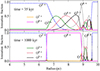 |
Fig. 19. Ionisation profiles of oxygen. The upper panel illustrates the NEQ case at t = 35 kyr, while the lower panel shows the IEQ state at t = 1000 kyr. |
There is a slight but noticeable difference in the ionisation of the gas in the freely expanding WR stellar wind region (r < 6.5 pc) between the NEQ and IEQ profiles, in that the NEQ calculation has about 5 per cent O3+ and 95 per cent O2+, whereas the IEQ calculation is effectively 100 per cent O2+. This difference arises because ionisation in this region is largely driven by photoionisation, and the photoionisation equilibrium timescale is longer than the expansion timescale of the wind.
In the shocked WR wind region (approximately r ∈ [6.5, 8.8] pc, cf. Fig. 13) where temperatures range from approximately 2 × 10⁷ K to 8.8 × 10⁷ K, oxygen is entirely in the O8+ state in the equilibrium case, a state that is less prevalent in the NEQ scenario. Since this region is dominated by collisional ionisation (thermal energy per particle is much larger than the photon energy from the stellar SED), the IEQ profile aligns with the one obtained under CIE conditions. For this temperature range, the CIE results show fully ionised oxygen, consistent with the IEQ profile obtained here. The NEQ profile can be understood based on the post-shock velocity (vps ≈ 1500/4 km s−1), temperature (T ≈ 108 K) and electron density (ne ∼ 0.003 cm−3). For this temperature the collisional ionisation rate-coefficient for O2+ is ζO, 2coll ≈ 10−8 cm3 s−1, giving an ionisation length scale ℓi = vps/(neζO, 2coll)≈0.3 pc. Figure 19 shows that the length scale for the O2+ abundance to decrease to half of its pre-shock value is ≈0.25 pc, comparable to our rough estimate. At this temperature, ζO, 2coll ≈ 2ζO, 3coll, so the O3+→O4+ transition has a somewhat larger length scale (the slower rate is somewhat compensated by the flow velocity decreasing with increasing r). In the NEQ calculation, the post-shock WR wind never reaches full ionisation over a length scale of nearly 2.5 pc. This is likely not directly observable because the density (and emission measure) of the gas is so low, but it may have an observable effect at the contact discontinuity where thermal conduction and turbulent mixing produce denser gas that can be detected in soft X-rays (Toalá & Arthur 2018).
The IEQ profile of the swept-up RSG wind differs from the corresponding NEQ case, although the dominant ion remains the same. In the NEQ scenario, the region is primarily composed of O6+ and O5+, with O6+ slightly prevailing over O5+. In contrast, the equilibrium case is dominated solely by O6+, with some O4+ and O3+ in the cooling layer behind the shock. This observation aligns with the CIE ionisation results (see Figure 1), where the O6+ ion fraction dominates within the temperature range of 3 × 10⁵ K to 2 × 10⁶ K. In the NEQ case the relatively long ionisation timescale results in significant O4+ and O5+ in the post-shock layer, together with O6+ with almost equal abundances.
We further compare the line luminosities between the NEQ and IEQ cases. Given that the density and temperature profiles remain identical in both scenarios, the ion fraction determines the line luminosity. As discussed in Sect. 4.2, the luminosity is predominantly determined by the mass density of the specific ion within the shell volume. Therefore, we anticipate distinct luminosities, as the ionisation profiles differ significantly in this region for both cases. Table 7 presents a comparison of line luminosities for the same transitions discussed in Sect. 4.2 for both the NEQ and IEQ cases. The O III and O IV lines exhibit lower luminosities in NEQ compared to IEQ, whereas the O VI and N IV lines show higher luminosities in NEQ. Notably, the O VIλ3811 and O VIλ3834 transitions display luminosities that are approximately 2.5 times greater in NEQ. The reduced luminosities of O III and O IV in NEQ are due to their higher mass densities in IEQ, as their ion fractions peak in regions of highest gas density. Conversely, the enhanced luminosities of O VI and N IV in NEQ are explained by their increased mass densities under non-equilibrium conditions.
Comparison of line luminosities for selected oxygen and nitrogen lines under non-equilibrium and equilibrium conditions.
5.3. Electron-ion temperature equilibration
We should caution that in the X-ray emitting regime, our single-fluid assumption that the electrons and ions have the same temperature may not be correct in the post-shock plasma. In collisionless shocks ions are heated more than electrons (Spitzer 1962), although the degree of the difference is still not well understood (Ghavamian et al. 2013) and measurements from supernova remnant shocks give different results compared with Solar Wind measurements and PIC simulations (Raymond et al. 2023). Nevertheless, the temperature ratio Te/Ti can be as low as 0.05–0.1 in supernova remnant shocks (Raymond et al. 2023). The electron-ion temperature equilibration via Coulomb collisions with protons has a timescale (Spitzer 1962; Ghavamian et al. 2013)
on substituting lnΛ = 30 for the Coulomb logarithm. For heavier ions τei is multiplied by mi/mpZi2 (e.g. Pollock et al. 2005), where mi and Zi are the mass and charge of ion i, respectively (that is, the timescale is shorter for heavy ions). This gives a length-scale in the shocked WR wind of the wind-wind simulation of ℓei ≈ 0.3 pc, comparable to the ionisation length-scale calculated above. Thus we may expect that X-ray emission from post-shock gas from fast shocks may not be accurately modelled in low-density plasma in the single-temperature approximation, and similarly the line emission in the soft X-ray O VII and O VIII lines. Observations show that for shock speeds vsh ≲ 400 km s−1 the electrons and ions have the same post-shock temperature (Ghavamian et al. 2013).
6. Conclusions
After extensive testing and validation, we have successfully integrated a solver for multi-ion non-equilibrium ionised plasmas into the radiation-MHD code, PION. This enhancement equips PION with the capability to spatially and temporally determine the distribution of ionisation levels for key elements – H, He, C, N, O, Ne, Si, S, and Fe – essential for radiative cooling and spectral line diagnostics. The solver incorporates collisional ionisation, photoionisation, charge-exchange reactions with H and He, and cosmic-ray ionisation of neutral species. It supports arbitrary elemental abundances for neutral and ionised gas (excluding molecular forms) and includes an enhanced non-equilibrium radiative cooling calculation. The ion-by-ion cooling curve, calculated based on instantaneous ion fractions, will facilitate more accurate modelling of ionisation in astrophysical scenarios where non-equilibrium ionisation conditions occur. This capability allows the module to predict spectral lines in the UV, optical, IR, and X-ray bands, even when the plasma is out of ionisation equilibrium, thus enabling more realistic comparison of simulations with observational data.
Various tests have been conducted to verify the solver’s accuracy. Collisional ionisation equilibrium was achieved, with the solver converging to the correct ionisation state, consistent with the results previously reported by, example, Sutherland & Dopita (1993). The solver reproduced the CIE cooling curve for both solar and Wolf-Rayet (WC) abundances, matching the findings reported by Sutherland & Dopita (1993) and Eatson et al. (2022a), respectively. When the same tests were performed with charge exchange enabled, the ionisation profiles displayed notable differences, closely matching the findings in the works of Gu et al. (2022) and Arnaud & Rothenflug (1985). Further validation was done by comparing the module’s results with both equilibrium and non-equilibrium calculations from existing literature. Several shock models, akin to Model E in (Raymond 1979), were simulated, including both adiabatic and non-adiabatic scenarios. Despite considerable resolution differences, the adiabatic shock tests showed excellent consistency in the ionisation profiles across low and high-resolution simulations. Non-adiabatic shock tests highlighted the non-equilibrium ionisation structure of the post-shock gas during radiative cooling and demonstrated the impact of charge exchange on ion abundances in cooling plasmas. Additionally, simulations of photoionised H II regions were conducted to validate the photoionisation subroutine in a multi-ion environment, following the HII40 Lexington benchmark and showing good overall agreement with results from the photoionisation code CLOUDY.
We conducted a comprehensive analysis of the performance and scalability of the MHD code with the new microphysics solver. The solver requires more computation with increasing Ntracer, with the runtime becoming predominantly influenced by the microphysics solver for Ntracer ≫ 10 and the cell update speed approaches a Ntracer−2 scaling. The wall-time decreases significantly with increasing OpenMP thread count, adhering to a Nthread−1 pattern up to 10−20 threads, and continues to show efficiency gains even with up to 30 threads. Overall, the code performance is commendable, facilitating detailed 2D simulations and enabling low-resolution 3D simulations. There is room for performance improvements by multithreading the microphysics integrator (CVODE) with OpenMP or GPU acceleration, and this will be explored in future work. The multi-ion module will form part of the next release of PION in 2025.
To demonstrate the capabilities of NEMO, we conducted 1D and 2D radiation hydrodynamics (RHD) simulations of the time-dependent spherical expansion of a WR wind into a pre-existing RSG wind, with strongly differing elemental abundances in the two winds, including photo-ionisation, collisional ionisation, recombination, and charge exchange reactions. We investigated the difference between our non-equilibrium results and the ionisation structure when integrated to equilibrium. There are significant differences that also give different line luminosities for bright nebular emission lines from soft X-ray to thermal IR. This application underscores the versatility of our module and showcases its effectiveness in modelling various ionisation processes in distinct regions. In future work we will apply this module to study supernova remnants, nebulae around WR stars and shocked plasma in colliding-wind binaries.
This rather crude approximation (and the associated heating rate in Eq. (14)) serves only to maintain a minimum electron fraction that improves the convergence of the non-equilbrium solver. It would need to be improved if one wished to carefully model low-temperature neutral and molecular gas where cosmic-ray ionisation and heating are important processes.
Acknowledgments
AM expresses his gratitude to Dr. Palmira Jiménez-Hernández for guiding him in the use of CLOUDY, which enabled him to obtain ionisation profiles of HII regions. AM acknowledges support from a Royal Society Enhanced Research Expenses grant (RF\ERE\210382). JM acknowledges support from a Royal Society–Science Foundation Ireland University Research Fellowship. MC acknowledges support from the Gates Cambridge Scholarship. TJH acknowledges funding from a Royal Society Dorothy Hodgkin Fellowship and UKRI guaranteed funding for a Horizon Europe ERC consolidator grant (EP/Y024710/1). This publication results from research conducted with the financial support of Taighde Éireann – Research Ireland under Grant numbers 20/RS-URF-R/3712, 22/RS-EA/3810. The authors are grateful to the referee for constructive comments that improved the quality of the manuscript.
References
- Abel, T., Norman, M., & Madau, P. 1999, ApJ, 523, 66 [NASA ADS] [CrossRef] [Google Scholar]
- Aldrovandi, S. M. V., & Pequignot, D. 1973, A&A, 25, 137 [NASA ADS] [Google Scholar]
- Allen, C. W. 1973, Astrophysical Quantities (London: University of London, Athlone Press) [Google Scholar]
- Arnaud, M., & Raymond, J. 1992, ApJ, 398, 394 [CrossRef] [Google Scholar]
- Arnaud, M., & Rothenflug, R. 1985, A&AS, 60, 425 [NASA ADS] [Google Scholar]
- Asplund, M., Grevesse, N., Sauval, A. J., & Scott, P. 2009, ARA&A, 47, 481 [NASA ADS] [CrossRef] [Google Scholar]
- Badnell, N. R. 2006, J. Phys. B At. Mol. Phys., 39, 4825 [NASA ADS] [CrossRef] [Google Scholar]
- Badnell, N. R., O’Mullane, M. G., Summers, H. P., et al. 2003, A&A, 406, 1151 [NASA ADS] [CrossRef] [EDP Sciences] [Google Scholar]
- Balos, C. J., Day, M., Esclapez, L., et al. 2024, arXiv e-prints [arXiv:2405.01713] [Google Scholar]
- Bisbas, T. G., Haworth, T. J., Williams, R. J. R., et al. 2015, MNRAS, 453, 1324 [NASA ADS] [CrossRef] [Google Scholar]
- Booth, R. A., Mohamed, S., & Podsiadlowski, P. 2016, MNRAS, 457, 822 [NASA ADS] [CrossRef] [Google Scholar]
- Butler, S. E., & Dalgarno, A. 1979, ApJ, 234, 765 [NASA ADS] [CrossRef] [Google Scholar]
- Butler, S. E., & Dalgarno, A. 1980, A&A, 85, 144 [NASA ADS] [Google Scholar]
- Butler, S. E., & Raymond, J. C. 1980, ApJ, 240, 680 [NASA ADS] [CrossRef] [Google Scholar]
- Butler, S. E., Heil, T. G., & Dalgarno, A. 1980, ApJ, 241, 442 [NASA ADS] [CrossRef] [Google Scholar]
- Castelli, F., & Kurucz, R. L. 2003, Proceedings of the 210th Symposium of the International Astronomical Union, A20 [Google Scholar]
- Chatzikos, M., Bianchi, S., Camilloni, F., et al. 2023, Rev. Mexicana Astron. Astrofis., 59, 327 [Google Scholar]
- Cohen, S. D., Hindmarsh, A. C., & Dubois, P. F. 1996, Comput. Phys., 10, 138 [NASA ADS] [CrossRef] [Google Scholar]
- de Avillez, M. A., & Breitschwerdt, D. 2012, ApJ, 756, L3 [NASA ADS] [CrossRef] [Google Scholar]
- Del Zanna, G., Dere, K. P., Young, P. R., Landi, E., & Mason, H. E. 2015, A&A, 582, A56 [NASA ADS] [CrossRef] [EDP Sciences] [Google Scholar]
- Del Zanna, G., Dere, K. P., Young, P. R., & Landi, E. 2021, ApJ, 909, 38 [NASA ADS] [CrossRef] [Google Scholar]
- Dere, K. P., Landi, E., Young, P. R., et al. 2009, A&A, 498, 915 [NASA ADS] [CrossRef] [EDP Sciences] [Google Scholar]
- Drake, G. W. F. 1986, Phys. Rev. A, 34, 2871 [NASA ADS] [CrossRef] [Google Scholar]
- Drake, G. W., Victor, G. A., & Dalgarno, A. 1969, Phys. Rev., 180, 25 [NASA ADS] [CrossRef] [Google Scholar]
- Eatson, J. W., Pittard, J. M., & Van Loo, S. 2022a, MNRAS, 516, 6132 [NASA ADS] [CrossRef] [Google Scholar]
- Eatson, J. W., Pittard, J. M., & Van Loo, S. 2022b, MNRAS, 517, 4705 [NASA ADS] [CrossRef] [Google Scholar]
- Ercolano, B., Barlow, M. J., Storey, P. J., & Liu, X.-W. 2003, MNRAS, 340, 1136 [NASA ADS] [CrossRef] [Google Scholar]
- Ferland, G. 1995, in The Analysis of Emission Lines: A Meeting in Honor of the 70th Birthdays of D. E. Osterbrock, eds. M. J. Seaton, R. Williams, & M. Livio, 83 [Google Scholar]
- Fichtner, Y. A., Mackey, J., Grassitelli, L., Romano-Díaz, E., & Porciani, C. 2024, A&A, 690, A72 [NASA ADS] [CrossRef] [EDP Sciences] [Google Scholar]
- Frank, A., & Mellema, G. 1994, A&A, 289, 937 [NASA ADS] [Google Scholar]
- Friedman, B., & DuCharme, G. 2017, J. Phys. B At. Mol. Phys., 50, 115202 [NASA ADS] [CrossRef] [Google Scholar]
- Friedrich, M. M., Mellema, G., Iliev, I. T., & Shapiro, P. R. 2012, MNRAS, 421, 2232 [NASA ADS] [CrossRef] [Google Scholar]
- Garcia-Segura, G., & Franco, J. 1996, ApJ, 469, 171 [NASA ADS] [CrossRef] [Google Scholar]
- García-Segura, G., Langer, N., & Mac Low, M. 1996, A&A, 316, 133 [NASA ADS] [Google Scholar]
- Gardner, D. J., Reynolds, D. R., Woodward, C. S., & Balos, C. J. 2022, ACM Trans. Math Software (TOMS), 48, 1 [CrossRef] [Google Scholar]
- Ghavamian, P., Schwartz, S. J., Mitchell, J., Masters, A., & Laming, J. M. 2013, Space Sci. Rev., 178, 633 [NASA ADS] [CrossRef] [Google Scholar]
- Glover, S. C. O., & Mac Low, M.-M. 2007, ApJS, 169, 239 [NASA ADS] [CrossRef] [Google Scholar]
- Glover, S. C. O., Federrath, C., Mac Low, M.-M., & Klessen, R. S. 2010, MNRAS, 404, 2 [NASA ADS] [Google Scholar]
- Gnat, O. 2017, ApJS, 228, 11 [NASA ADS] [CrossRef] [Google Scholar]
- Gnat, O., & Sternberg, A. 2007, ApJS, 168, 213 [NASA ADS] [CrossRef] [Google Scholar]
- Goldman, S. P., & Drake, G. W. F. 1981, Phys. Rev. A, 24, 183 [NASA ADS] [CrossRef] [Google Scholar]
- Goldsmith, P. F., & Langer, W. D. 1978, ApJ, 222, 881 [Google Scholar]
- Gong, M., Ostriker, E. C., & Wolfire, M. G. 2017, ApJ, 843, 38 [NASA ADS] [CrossRef] [Google Scholar]
- Grassi, T., Bovino, S., Schleicher, D. R. G., et al. 2014, MNRAS, 439, 2386 [Google Scholar]
- Gu, L., Shah, C., & Zhang, R. 2022, Sensors, 22, 752 [NASA ADS] [CrossRef] [Google Scholar]
- Hamann, W. R., & Gräfener, G. 2004, A&A, 427, 697 [NASA ADS] [CrossRef] [EDP Sciences] [Google Scholar]
- Harries, T. J., Haworth, T. J., Acreman, D., Ali, A., & Douglas, T. 2019, Astron. Comput., 27, 63 [NASA ADS] [CrossRef] [Google Scholar]
- Haworth, T. J., & Harries, T. J. 2012, MNRAS, 420, 562 [NASA ADS] [CrossRef] [Google Scholar]
- Henney, W. J., Arthur, S. J., de Colle, F., & Mellema, G. 2009, MNRAS, 398, 157 [NASA ADS] [CrossRef] [Google Scholar]
- Hindmarsh, A. C., Brown, P. N., Grant, K. E., et al. 2005, ACM Trans. Math. Software (TOMS), 31, 363 [CrossRef] [Google Scholar]
- Hui, L., & Gnedin, N. Y. 1997, MNRAS, 292, 27 [Google Scholar]
- Hummer, D. G. 1994, MNRAS, 268, 109 [NASA ADS] [CrossRef] [Google Scholar]
- Karzas, W. J., & Latter, R. 1961, ApJS, 6, 167 [Google Scholar]
- Kaur, J., Gorczyca, T. W., & Badnell, N. R. 2018, A&A, 610, A41 [NASA ADS] [CrossRef] [EDP Sciences] [Google Scholar]
- Kingdon, J. B., & Ferland, G. J. 1996, ApJS, 106, 205 [NASA ADS] [CrossRef] [Google Scholar]
- Koo, B.-C., & McKee, C. F. 1992, ApJ, 388, 103 [NASA ADS] [CrossRef] [Google Scholar]
- Lasker, B. M. 1966, ApJ, 143, 700 [CrossRef] [Google Scholar]
- Lim, A. J., & Mellema, G. 2003, A&A, 405, 189 [NASA ADS] [CrossRef] [EDP Sciences] [Google Scholar]
- Mackey, J. 2012, A&A, 539, A147 [NASA ADS] [CrossRef] [EDP Sciences] [Google Scholar]
- Mackey, J., & Lim, A. J. 2010, MNRAS, 403, 714 [NASA ADS] [CrossRef] [Google Scholar]
- Mackey, J., & Lim, A. J. 2011, MNRAS, 412, 2079 [NASA ADS] [CrossRef] [Google Scholar]
- Mackey, J., Langer, N., & Gvaramadze, V. V. 2013, MNRAS, 436, 859 [NASA ADS] [CrossRef] [Google Scholar]
- Mackey, J., Gvaramadze, V. V., Mohamed, S., & Langer, N. 2015, A&A, 573, A10 [NASA ADS] [CrossRef] [EDP Sciences] [Google Scholar]
- Mackey, J., Green, S., Moutzouri, M., et al. 2021, MNRAS, 504, 983 [NASA ADS] [CrossRef] [Google Scholar]
- Mackey, J., Jones, T. A. K., Brose, R., et al. 2023, MNRAS, 526, 3099 [NASA ADS] [CrossRef] [Google Scholar]
- McCarroll, R., & Valiron, P. 1976, A&A, 53, 83 [NASA ADS] [Google Scholar]
- Mellema, G. 1995, MNRAS, 277, 173 [NASA ADS] [Google Scholar]
- Mellema, G., & Lundqvist, P. 2002, A&A, 394, 901 [NASA ADS] [CrossRef] [EDP Sciences] [Google Scholar]
- Mellema, G., Iliev, I., Alvarez, M., & Shapiro, P. 2006, New Astron., 11, 374 [NASA ADS] [CrossRef] [Google Scholar]
- Mignone, A., Bodo, G., Massaglia, S., et al. 2007, ApJS, 170, 228 [Google Scholar]
- Nelson, R. P., & Langer, W. D. 1997, ApJ, 482, 796 [NASA ADS] [CrossRef] [Google Scholar]
- Neufeld, D. A., & Dalgarno, A. 1987, Phys. Rev. A, 35, 3142 [NASA ADS] [CrossRef] [Google Scholar]
- Oppenheimer, B. D., & Schaye, J. 2013, MNRAS, 434, 1043 [CrossRef] [Google Scholar]
- Parkin, E. R., Pittard, J. M., Corcoran, M. F., & Hamaguchi, K. 2011, ApJ, 726, 105 [CrossRef] [Google Scholar]
- Parpia, F. A., & Johnson, W. R. 1982, Phys. Rev. A, 26, 1142 [NASA ADS] [CrossRef] [Google Scholar]
- Pequignot, D., Petitjean, P., & Boisson, C. 1991, A&A, 251, 680 [NASA ADS] [Google Scholar]
- Plewa, T., & Müller, E. 1999, A&A, 342, 179 [NASA ADS] [Google Scholar]
- Pollock, A. M. T., Corcoran, M. F., Stevens, I. R., & Williams, P. M. 2005, ApJ, 629, 482 [Google Scholar]
- Raga, A. C., Mellema, G., & Lundqvist, P. 1997, ApJS, 109, 517 [CrossRef] [Google Scholar]
- Raga, A. C., Mellema, G., Arthur, S. J., et al. 1999, Rev. Mexicana Astron. Astrofis., 35, 123 [Google Scholar]
- Raymond, J. C. 1979, ApJS, 39, 1 [NASA ADS] [CrossRef] [Google Scholar]
- Raymond, J. C., Ghavamian, P., Bohdan, A., et al. 2023, ApJ, 949, 50 [NASA ADS] [CrossRef] [Google Scholar]
- Richings, A. J., & Schaye, J. 2016, MNRAS, 458, 270 [NASA ADS] [CrossRef] [Google Scholar]
- Richings, A. J., Schaye, J., & Oppenheimer, B. D. 2014a, MNRAS, 440, 3349 [CrossRef] [Google Scholar]
- Richings, A. J., Schaye, J., & Oppenheimer, B. D. 2014b, MNRAS, 442, 2780 [Google Scholar]
- Rybicki, G. B., & Lightman, A. P. 1986, Radiative Processes in Astrophysics (Wiley-VCH) [Google Scholar]
- Sander, A., Hamann, W. R., & Todt, H. 2012, A&A, 540, A144 [NASA ADS] [CrossRef] [EDP Sciences] [Google Scholar]
- Sarkar, K. C., Sternberg, A., & Gnat, O. 2021, MNRAS, 503, 5807 [CrossRef] [Google Scholar]
- Schaye, J., Crain, R. A., Bower, R. G., et al. 2015, MNRAS, 446, 521 [Google Scholar]
- Smith, B. D., Bryan, G. L., Glover, S. C. O., et al. 2017, MNRAS, 466, 2217 [NASA ADS] [CrossRef] [Google Scholar]
- Spitzer, L. 1962, Physics of Fully Ionized Gases (Interscience Publishers) [Google Scholar]
- Steigman, G. 1975, ApJ, 199, 336 [CrossRef] [Google Scholar]
- Štofanová, L., Kaastra, J., Mehdipour, M., & de Plaa, J. 2021, A&A, 655, A2 [NASA ADS] [CrossRef] [EDP Sciences] [Google Scholar]
- Sutherland, R. S., & Dopita, M. A. 1993, ApJS, 88, 253 [Google Scholar]
- Teşileanu, O., Mignone, A., & Massaglia, S. 2008, A&A, 488, 429 [NASA ADS] [CrossRef] [EDP Sciences] [Google Scholar]
- Toalá, J. A., & Arthur, S. J. 2018, MNRAS, 478, 1218 [CrossRef] [Google Scholar]
- Todt, H., Sander, A., Hainich, R., et al. 2015, A&A, 579, A75 [NASA ADS] [CrossRef] [EDP Sciences] [Google Scholar]
- Vandenbroucke, B., & Wood, K. 2018, Astron. Comput., 23, 40 [NASA ADS] [CrossRef] [Google Scholar]
- Verner, D. A., & Ferland, G. J. 1996, ApJS, 103, 467 [NASA ADS] [CrossRef] [Google Scholar]
- Verner, D. A., Ferland, G. J., Korista, K. T., & Yakovlev, D. G. 1996, ApJ, 465, 487 [Google Scholar]
- Voronov, G. S. 1997, At. Data Nucl Data Tables, 65, 1 [CrossRef] [Google Scholar]
- Walch, S., Girichidis, P., Naab, T., et al. 2015, MNRAS, 454, 238 [Google Scholar]
- Wiersma, R. P. C., Schaye, J., & Smith, B. D. 2009, MNRAS, 393, 99 [NASA ADS] [CrossRef] [Google Scholar]
- Wünsch, R., Walch, S., Dinnbier, F., et al. 2021, MNRAS, 505, 3730 [CrossRef] [Google Scholar]
- Young, P. R., Del Zanna, G., Landi, E., et al. 2003, ApJS, 144, 135 [CrossRef] [Google Scholar]
- Zatsarinny, O., Gorczyca, T. W., Korista, K. T., Badnell, N. R., & Savin, D. W. 2003, A&A, 412, 587 [NASA ADS] [CrossRef] [EDP Sciences] [Google Scholar]
- Zygelman, B., & Dalgarno, A. 1990, ApJ, 365, 239 [NASA ADS] [CrossRef] [Google Scholar]
Appendix A: Catalogue of charge exchange reactions
All recombination and ionisation charge exchange reactions involving relevant ions with H and He, as incorporated in NEMO, are presented in Tables A.1 and A.2.
List of recombination charge exchange reactions.
List of ionisation charge exchange reactions.
Appendix B: Convergence of photoionisation and photo-heating with varying energy bin resolutions
Energy Binning for Varying Bin Counts
To test how sensitive our photoionisation results are to the energy binning of the radiation field, we recomputed the static H II region simulations of section 3.4 with the standard setting of Nb = 15 energy bins, plus coarser binning of Nb = 4 and 8, and finer binning with Nb = 28 and 64. The energy boundaries of the bins are given in Table B.1. Results equivalent to those in Figs. 10 to 12 are plotted in Figs. B.1 to B.3, respectively.
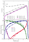 |
Fig. B.1. As Fig. 10, but without the middle panel, and showing convergence of temperature and ionisation profiles with number of energy bins for the radiation field, Nb. |
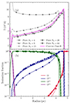 |
Fig. B.2. As Fig. 11, but without the middle panel, and showing convergence of temperature and ionisation profiles with number of energy bins for the radiation field, Nb. |
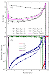 |
Fig. B.3. As Fig. 12, but without the middle panel, and showing convergence of temperature and ionisation profiles with number of energy bins for the radiation field, Nb. |
These plots show that Nb = 4 is clearly insufficient for both the temperature and ionisation structure of the H II region in all three cases. For the ionisation structure, Nb = 8 is probably acceptable and Nb= 15, 28 and 64 are indistinguishable. This is not the case for the temperature structure, however, which is converging only at first order with Nb, and Nb = 8 is quite far from the converged solution. Results with the default binning of Nb = 15 are reasonably close to converged. The radiation spectrum is assumed piecewise constant in our discretisation and so first-order convergence is the expected behaviour. Better convergence would be obtained with a piecewise linear interpolation of the spectrum because the mean heating rate per photon in a bin would be better approximated when the spectrum is steep (which is usually the case in the EUV).
With the finest energy binning, Nb = 64, the results for temperature and ionisation structure converge very well to the CLOUDY Case-B results for the low density simulation (Fig. B.1), but less so for higher density (Fig. B.3), as already discussed in section 3.4. The reasons for this are not completely clear, but our radiative transfer scheme is much more rudimentary than that of CLOUDY and we suspect that this is the reason, although differences in atomic data may also play a role.
All Tables
Verner-Ferland fit parameters (A, B, T0, T1) for the S1+ ion, determined by optimal fitting of the Verner-Ferland model onto the Aldrovandi & Pequignot fit with Arad = 4.1 × 10⁻¹³ and η = 0.630.
Mass fractions for Solar abundances (Asplund et al. 2009) and for the wind of a WR star of type WC9 (from Eatson et al. 2022a).
Simulation parameters used for the H II region test with the HII40 Lexington benchmark model (Ferland 1995; Ercolano et al. 2003; Haworth & Harries 2012).
Energy bins for the radiation field for photoionisation calculations, chosen to line up with ionisation thresholds of the modelled ions, as much as possible.
Parameters for 1D MHD Simulation of Wind-Wind Interaction: Ionising Source, Stellar Wind, and CSM.
Comparison of line luminosities for selected oxygen and nitrogen lines under non-equilibrium and equilibrium conditions.
All Figures
|
Fig. 1. Ionisation fractions of the elements included in our microphysics module under CIE conditions, obtained by integrating until equilibrium is obtained. The first panel depicts the ionisation levels of H (black), He (red), and C (blue); the second panel the ionisation levels of N (black), O (red), and Ne (blue); the third panel the ionisation levels of Si (black) and S (red); and the fourth panel the ionisation levels of Fe (black). |
| In the text | |
|
Fig. 2. Radiative cooling rates under CIE conditions obtained with our new microphysics module, including elemental contributions Lκ (scaled by (mH/ρ)2 in the first, second, and fourth panels, and by (nenH)−1 in the third panel, respectively) and net cooling function for Solar and WC abundances. Top: elemental contribution of the cooling curve for solar abundances, as specified in Table 2. The black solid line represents the net cooling curve. Second: elemental contribution of the cooling curve for WC abundances, as indicated in Table 2. The blue solid line represents the net cooling curve. Third: comparison of the net cooling curves for solar abundances with those derived by Sutherland & Dopita (1993) and Wiersma et al. (2009). Bottom: net cooling curves for WC abundances compared with the cooling function obtained by Eatson et al. (2022a). |
| In the text | |
|
Fig. 3. Comparison of CIE balance for N, O, Ne, and Si incorporating and omitting charge exchange (CX) reactions with H and He. Solid curves represent ionisation fractions with charge exchange calculations, while dashed curves represent ionisation fractions without charge exchange reactions. |
| In the text | |
|
Fig. 4. Flow quantities of an adiabatic shock generated by gas flowing at a velocity of 100 km s−1. The simulation employs 10 240 grid cells and not all of the domain is shown. |
| In the text | |
|
Fig. 5. Spatial profiles of ion fractions for H, He, C, N, O, and Ne across the shock front for shock test 1, comparing the low (dashed lines) and high (solid lines) resolution simulations. The flow moves from right to left, with the shock positioned at the plot’s right-hand boundary. The plot depicts only the downstream region. |
| In the text | |
|
Fig. 6. Illustration of the flow structure in pre-shock gas interacting with the shock front. The top panel exhibits temperature (red-solid curve) and density (blue-dashed curve) profiles at t1 = 1.2945 × 10⁴ years, while the bottom panel presents the same at a later time, t = 1.2799 × 10⁵ years, highlighting the interplay between Chianti cooling data and gas dynamics. |
| In the text | |
|
Fig. 7. Ionisation fractions of H, He, and C within the cooling region of non-adiabatic shock test 2, revealing non-equilibrium dynamics of chemical species at later time, t = 1.2799 × 10⁵ years. |
| In the text | |
|
Fig. 8. Spatial profiles of ion fractions for different ionisation levels of Si across the shock front in non-adiabatic flows at velocities of 1000 km s−1 (top panel) and 3000 km s−1 (bottom panel). |
| In the text | |
|
Fig. 9. Temperature and ionisation profiles of the shocked gas with and without charge transfer processes. The top panel shows temperature as a function of position, with the shock off the grid to the right, and the flow from right to left. The temperature profile with and without charge-exchange is almost identical. The bottom panel shows the ionisation fractions of oxygen, emphasizing the significance of charge transfer reactions for the oxygen ionisation state, especially below 6 × 10³ K. |
| In the text | |
|
Fig. 10. Photoionisation equilibrium calculation for the temperature and ionisation state of a static H II region for a H number density nH = 10 cm−3: (a) gas temperature vs. radius for 3 different calculations: dotted-red line obtained with CLOUDY, dashed-red line CLOUDY with the Case-B setting and solid-blue line shows the result with PION using the On-the-Spot approximation (see text for details); (b) ionisation state of H and He as a function of radius: solid lines are results obtained with PION, dotted lines with CLOUDY and dashed lines CLOUDY+CaseB; and (c) as (b) but showing ionisation state of O as a function of radius. |
| In the text | |
|
Fig. 11. Photoionisation equilibrium calculation for the temperature and ionisation state of a static H II region for a H number density nH = 100 cm−3 (The Lexington HII40 benchmark test): panels (a), (b), and (c) as for Fig. 10 except that panel (a) also includes the result from TORUS. |
| In the text | |
|
Fig. 12. Photoionisation equilibrium calculation for the temperature and ionisation state of a static H II region for a H number density nH = 1000 cm−3: panels (a), (b), and (c) as for Fig. 10. |
| In the text | |
|
Fig. 13. Snapshot from 1D simulation of wind-wind interaction from a WR wind expanding into a pre-existing RSG wind from a previous evolutionary phase. The top panel displays the flow quantities, and the subsequent panels show the ionisation profiles of H, He, C, N, and O, all at a time 35 kyr after the initiation of the WR wind. |
| In the text | |
|
Fig. 14. Time evolution of luminosity for selected oxygen and nitrogen emission lines for the 1D wind-wind simulation in Sect. 4, calculated as described in Sect. 4.2. The forward shock leaves the domain at around 45 kyr, and the associated sharp drop in some line luminosities is therefore artificial. |
| In the text | |
|
Fig. 15. Snapshot from a two-dimensional simulation captures the interaction between the WR wind and the remnant wind from the earlier RSG phase. The image shows the flow quantities 23.36 kyr after the onset of the WR wind, with the star located at the origin. The top panel shows log10 of gas density (g cm−3) according to the colour scale shown, where brighter yellow regions indicate higher density, and darker purples represent lower density. The bottom panel shows log10 of temperature (in K) according to the colour scale displayed beside the plot. |
| In the text | |
|
Fig. 16. Ionisation profile of O2+ to O7+ ions from a two-dimensional simulation of the interaction between the WR wind and the remnant RSG wind, shown 23.36 kyr after the onset of the WR wind. The panels illustrate the ionisation fraction, YO, i on a linear scale, with white representing a oxygen completely in this ionisation state (YO, i = 1) and black denoting the zero abundance (YO, i = 0). The colour scale is shown at the far right of the plot. |
| In the text | |
|
Fig. 17. Relation between simulation speed and the number of tracers (elements plus their ions). The upper plot shows the wall-time of a 1D simulation using from one to nine elements, with either 10 or 15 OpenMP threads on 10 or 15 cores. The lower panel shows the same data, calculating the number of cells updated per core per second. This 1D shock calculation did not include photoionisation or charge-exchange reactions (see text for details). |
| In the text | |
|
Fig. 18. Parallel scaling of the same 1D shock test as Fig. 17 (except that now charge-exchange reactions are included), showing the simulation wall-time as a function of the number of OpenMP threads (and cores) used for the calculation. This is compared with the ideal speedup of Nthread−1 (dashed line). |
| In the text | |
|
Fig. 19. Ionisation profiles of oxygen. The upper panel illustrates the NEQ case at t = 35 kyr, while the lower panel shows the IEQ state at t = 1000 kyr. |
| In the text | |
|
Fig. B.1. As Fig. 10, but without the middle panel, and showing convergence of temperature and ionisation profiles with number of energy bins for the radiation field, Nb. |
| In the text | |
|
Fig. B.2. As Fig. 11, but without the middle panel, and showing convergence of temperature and ionisation profiles with number of energy bins for the radiation field, Nb. |
| In the text | |
|
Fig. B.3. As Fig. 12, but without the middle panel, and showing convergence of temperature and ionisation profiles with number of energy bins for the radiation field, Nb. |
| In the text | |
Current usage metrics show cumulative count of Article Views (full-text article views including HTML views, PDF and ePub downloads, according to the available data) and Abstracts Views on Vision4Press platform.
Data correspond to usage on the plateform after 2015. The current usage metrics is available 48-96 hours after online publication and is updated daily on week days.
Initial download of the metrics may take a while.