| Issue |
A&A
Volume 693, January 2025
|
|
|---|---|---|
| Article Number | L12 | |
| Number of page(s) | 6 | |
| Section | Letters to the Editor | |
| DOI | https://doi.org/10.1051/0004-6361/202451372 | |
| Published online | 13 January 2025 | |
Letter to the Editor
Revealing super-adiabatic features of interplanetary coronal mass ejections at 1 au
1
Space Sciences Laboratory, University of California, Berkeley, 7 Gauss Way, CA 94720, USA
2
William B. Hanson Center for Space Sciences, University of Texas at Dallas, Richardson, TX, USA
3
Department of Space and Climate Physics, Mullard Space Science Laboratory, University College London, Holmbury St. Mary, Dorking, UK
4
University Department of Physics, University of Mumbai, Vidyanagari, Santacruz (E), Mumbai 400098, India
⋆ Corresponding author; This email address is being protected from spambots. You need JavaScript enabled to view it.
Received:
3
July
2024
Accepted:
8
December
2024
Abstract
Interplanetary coronal mass ejections (ICMEs) are large-scale, coherent magnetic structures that play a pivotal role in heliospheric dynamics and space weather phenomena. Although thermodynamic analyses of ICME magnetic obstacles (MOs) at 1 au generally reveal adiabatic characteristics, the broader thermodynamic processes and associated plasma heating and cooling mechanisms remain insufficiently understood. In this study we analysed 473 ICME MOs observed at 1 au by the ACE spacecraft, utilising polytropic analysis to determine the polytropic index, α, for these structures. We identified 25 ICME MOs in which plasma protons exhibit a polytropic index α ≳ 2.00, with a mean value of 2.14 ± 0.07, indicating super-adiabatic behaviour. We also observed evidence of 12 isothermal (α ∼ 1) and 45 adiabatic (α ∼ 5/3) ICME MOs. Furthermore, in the case of super-adiabatic ICME MOs, we observe that all the total supplied heat is efficiently utilised to accomplish work in the surrounding environment, assuming the protons have three effective kinetic degrees of freedom. Therefore, as they expand, these ICMEs MOs cool faster than the adiabatic plasma. Our findings are critical to comprehending the dynamic evolution of ICMEs in interplanetary space and the energy-exchange mechanisms involved.
Key words: plasmas / turbulence / Sun: coronal mass ejections (CMEs) / Sun: magnetic fields / solar wind
© The Authors 2025
 Open Access article, published by EDP Sciences, under the terms of the Creative Commons Attribution License (https://creativecommons.org/licenses/by/4.0), which permits unrestricted use, distribution, and reproduction in any medium, provided the original work is properly cited.
This article is published in open access under the Subscribe to Open model. This email address is being protected from spambots. You need JavaScript enabled to view it. to support open access publication.
1. Introduction
Coronal mass ejections (CMEs) are large-scale blobs of magnetised plasma ejected from solar corona into interplanetary space (Webb & Howard 2012; Howard 2011). CMEs are responsible for the most severe space weather disruptions and significant rearrangements of the coronal magnetic field (Schwenn 2006; Pulkkinen 2007; Bothmer & Daglis 2007; Shaikh et al. 2018; Moldwin 2022; Ghag et al. 2023; Raghav et al. 2023). The interplanetary counterpart of CMEs are interplanetary coronal mass ejections (ICMEs; Gopalswamy 2006; Zurbuchen & Richardson 2006). In situ observations show that ICMEs consist of three distinct regions: the shock, the sheath, and the magnetic obstacle (MO; Zurbuchen & Richardson 2006; Richardson & Cane 2010; Nieves-Chinchilla et al. 2018; Shaikh et al. 2020; Shaikh & Raghav 2022; Good et al. 2022). A MO can consist of a single magnetic flux rope (MFR), multiple MFRs, or none (Jian et al. 2006; Nieves-Chinchilla et al. 2016, 2018, 2019). The MFR has a coherent magnetic field structure with bundles of helical magnetic field lines coiling around a specific axis (Burlaga et al. 1981; Lepping et al. 1990; Good et al. 2022). A MFR exhibiting a smooth magnetic field rotation, low plasma beta, low plasma density, and low temperature is referred to as a magnetic cloud (MC; Klein & Burlaga 1982; Zurbuchen & Richardson 2006; Raghav & Shaikh 2020; Shaikh & Raghav 2022), while MFRs not exhibiting smooth magnetic field rotation are called non-MCs (Wang et al. 2019; Richardson & Cane 2010; Chi et al. 2016). Moreover, it has been proposed that all ICMEs near 1 au have a MFR structure (Song et al. 2020). To minimise confusion, we use the term ‘MO’ to denote the ICME magnetic structure analysed in this Letter. Our knowledge of the thermodynamic properties of ICME plasma is still limited and requires further research (Forsyth et al. 2006; Webb & Howard 2012). Analysing ICME plasma heating and cooling processes is crucial for improving space weather forecasts and understanding solar-terrestrial interactions.
Most studies of CMEs have relied on white light imaging techniques, which provide only plasma density estimates (Howard 2011). Observations of extreme-UV spectral observations aboard the Solar and Heliospheric Observatory (SOHO) spacecraft have provided only a few insights into the thermodynamics of CMEs (Akmal et al. 2001; Bemporad & Mancuso 2010). The polytropic approximation has often been used to model the heating and cooling of expanding plasma in the heliosphere (e.g. Osherovich et al. 1993; Nicolaou et al. 2014, 2020, 2023; Livadiotis 2019a; Dayeh & Livadiotis 2022). Different values of the polytropic index, α, have been used and resulted in different calculated plasma heating rates and plasma evolution (Nicolaou et al. 2019, 2020; Shaikh et al. 2023). The polytropic approximation for the energy equation has also often been used to investigate ICME dynamics using global magnetohydrodynamic modelling (Riley et al. 2003; Manchester et al. 2004). Gibson & Low (1998) used α = 4/3 for their analytical model describing the evolution of a 3D CME. Chen (1996) and Krall et al. (2000) used α = 1.2 in their theoretical model describing ICME initiation and propagation. The remote sensing observation-based flux rope internal state model shows that the dynamics of CME plasma can exhibit polytropic index values from 1.3 to 1.9 over the range of radial distances from 6 to 230 R⊙ (Mishra & Wang 2018; Mishra et al. 2020). Thus, most observational and theoretical studies suggest that the polytropic index of CME plasma is in the range 1 ≲ α ≲ 5/3; we note that α = 1 and 5/3 respectively correspond to isothermal and adiabatic expansion.
Several attempts have been made to estimate the polytropic index of ICME MC plasma using in situ observations of plasma density and temperature. It has been found that the polytropic index of electrons within ICME MCs is less than 1, αe < 1 (e.g. Osherovich et al. 1993, 1998, 1999; Farrugia et al. 1995; Sittler & Burlaga 1998), though several other studies reported αe > 1 (e.g. Gosling 1999; Gosling et al. 2001). Osherovich et al. (1993) found that the polytropic index of protons, αp, within ICME MCs is between 1.1 and 1.3. Liu et al. (2006) reported αp = 1.3 within the expanding ICME flux ropes between 0.3 and 20 au. Moreover, densities and magnetic fields have been observed to decrease faster in ICME MFRs than in ambient solar wind, but the temperature decreases are slower, implying an extra heating of plasma in ICME MFRs compared to ambient solar wind (Wang et al. 2005; Liu et al. 2006, 2005). The mechanism of this extra heating is still not established. Moreover, Liu et al. (2005) also found that the polytropic index of protons is around 1.15, while the polytropic index for electrons is around 0.73.
The plasma heating within ICME MFRs can occur via several mechanisms, including current sheet (e.g. Ciaravella & Raymond 2008; Mei et al. 2012; Owens 2009), kink instability (e.g. Huang et al. 2006; Butler et al. 2022), magnetic reconnection (e.g. McComas et al. 1994; Murphy et al. 2011; Gosling 2012), and heating by plasma turbulence (e.g. Li et al. 2017; Fan et al. 2018). Nevertheless, only a few studies have addressed the heating and cooling of ICME plasma in the course of their propagation (e.g. Mishra & Wang 2018; Mishra et al. 2020; Liu et al. 2006; Osherovich et al. 1993). Traditionally, it was believed that ICME plasma behaves adiabatically near the Sun and isothermally at 1 au (Mishra & Wang 2018; Osherovich et al. 1993; Liu et al. 2006). A statistical study by Dayeh & Livadiotis (2022) shows that plasma expansion within ICME MFRs is nearly adiabatic at 1 au with α ∼ 1.5. Recently, Ghag et al. (2024) performed a multi-spacecraft (longitudinally separated) analysis of ICME MFRs and revealed nearly isothermal plasma expansion. We believe that further analysis of plasma thermodynamics is currently needed to explore the efficiency of plasma heating and cooling within ICME MFRs in greater detail.
Most spacecraft observations indicate that the expansion of ICME plasma is either isothermal or adiabatic. Models and simulations also assume isothermal or adiabatic evolution of ICME plasma throughout the heliosphere (see e.g. Chen 1996, 2011, 2017; Riley et al. 2003; Mishra et al. 2020, and references therein). This may underestimate or overestimate the energetics of ICME; thus, a more accurate analysis of the polytropic index is necessary. We applied the standard analysis to estimate the polytropic index for 473 ICME MOs to examine a subset of atypical ICME MOs that exhibit super-adiabatic behaviour at 1 au.
2. Data and methodology
We used in situ level 2 data with 64 s temporal resolution from the Advanced Composition Explorer (ACE) spacecraft located at 1 au1. The magnetic field data (Bx, By, Bz) were provided by the Magnetic Field Experiment (MAG) instrument (Smith et al. 1998), whereas plasma parameters (proton velocity, Vp, density, Np, and temperature, Tp) were provided by the Solar Wind Electron, Proton, and Alpha Monitor (SWEPAM) instrument (McComas et al. 1998). We analysed 473 ICMEs observed from 1998 to 2017 and extracted them from the catalogue available in Richardson & Cane (2024). The ACE spacecraft has been positioned at L1 since its launch in 1997. The long-term data from ACE comprise consistent and accurate observations of interplanetary conditions at 1 au. The robustness and calibration of these instruments have been thoroughly validated in numerous prior studies2, giving us confidence in the reliability of the data used for understanding the thermodynamic behaviour of ICME MOs. The present study does not explore the dependence of the thermodynamic behaviour of ICME MOs on solar cycles, although it includes data from solar cycle 23 and part of solar cycle 24.
The composition of ICMEs is typically rich in heavier ions such as helium (He2+) and features higher charge states of ions like oxygen (O7+/O6+) and iron (Fe10+/Fe13+); however, protons still comprise the majority of the make-up, accounting for about 90–95% of the population of ions by number (Richardson & Cane 2010; Zurbuchen & Richardson 2006; Song et al. 2021). Since protons constitute the most dominant population, our initial focus was their analysis, but this does not mean the thermodynamics of other particles are unimportant. For each ICME MO, we estimated the polytropic index for protons. The analysis of plasma within MOs, which are ordered magnetic structures, allowed us to minimise the mixing of distinct plasma streamlines; this is required for a reliable estimate of the polytropic index. For ideal gases, the polytropic law for protons can be written as follows (Chandrasekhar 1933; Parker 1965; Livadiotis 2018a,b):
 (1)
(1)
where Pth = NpkBTp is the proton thermal pressure (kB is the Boltzmann constant) and α is the polytropic index. We note that α should not be confused with the specific heat ratio γ = cp/cv = 1 + 2/f, where f is the number of kinetic degrees of freedom (e.g. Totten et al. 1995; Nicolaou et al. 2020; Shaikh et al. 2023; Shaikh & Vichare 2022). Only in the case of adiabatic evolution do we have α = γ. The proton temperature increases with the radial distance from the Sun in the case of α < 1, remains constant for α = 1, and decreases with the radial distance in the case of 1 < α < γ, though not as rapidly as in the adiabatic case (Chen & Garren 1993). Equation (1) can be rewritten as follows:
 (2)
(2)
where F is a constant. We fitted Eq. (2) to scattered data of log10Pth versus log10Np. The slope of the best fit delivers the value of α, while the point where it crosses the y-axis determines log10F. We also estimate plasma entropy S = 1.5 kBln(Pth/Npα) (here, ln means natural logarithm) to be presented in kB units. The entropy is constant in the case of adiabatic expansion.
3. Analysis and discussion
We estimated the polytropic index of protons for each of the 473 selected ICME MOs. We also determined averaged plasma parameters (Vp, Np, Tp), magnetic field strength BT, and plasma proton beta βp = 2 μ0Pth/BT2. Figure 1 shows an ICME observed by ACE at 1 au from December 16, 2006, 17:20:00 to December 17, 2006, 17:00:00 UTC. The panels present the magnetic field magnitude and its components followed by plasma parameters. The ICME sheath region is characterised by enhanced magnetic field magnitude, proton moments, magnetic field fluctuations, and proton beta compared to the ambient solar wind. The ICME MO region is characterised by an ordered and smooth magnetic field and low proton temperatures, low densities, and a low magnetic field fluctuation intensity compared to the sheath. The averaged plasma parameters within the ICME MO region are BT ≈ 4.3 nT, Vp ≈ 585 km/s, Np ≈ 2.6 cm−3, Tp ≈ 5.5 × 10⁴ K, and βp ≈ 0.27. The bottom panel presents the analysis of the polytropic index of the proton population within the ICME MO region. The linear fit of log10Pth to log10Np reveals a slope of α = 2.02 ± 0.04 and intercept log10F = −8.40 ± 0.04, while the Pearson correlation coefficient is about 0.95.
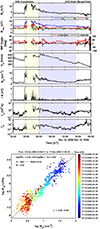 |
Fig. 1. ICME event observed by ACE from December 16 to December 17, 2006. Upper panel, from top to bottom: Temporal variation in the total IMF (the interplanetary magnetic field) BT, IMF vector Bvec = (Bx, By, Bz), azimuthal (ϕ = tan−1(By/Bx)) and elevation ( |
We performed a similar analysis for the other ICME MOs and found 12 events exhibiting isothermal behaviour (α ≈ 1), 45 events exhibiting adiabatic behaviour (α ≈ 5/3), and 25 events with 1.8 < α < 2.86. We note that only ICME MOs with a high Pearson correlation coefficient (≳0.90) and a clear visual trend of log10Pth versus log10Np were considered (Table B.1). For the other ICME MOs, the plasma either shows a complex relation between log10Pth and log10Np or has a large data gap, making the power-law fit inappropriate.
Figure 2 presents the proton polytropic index, α, distribution for the 82 ICME MOs. There are 12 ICME MOs that have isothermal α ∼ 1 (0.8 < α < 1.3) characteristics, with an average α = 1.10. There are 45 that show adiabatic α ∼ 5/3 (1.3 < α < 1.75) behaviour, with an average α = 1.52. For the 25 ICME MOs with α > 1.8, the mean and median values of the distribution are 2.14 and 2.09, respectively. These MOs exhibit super-adiabatic behaviour, assuming that there are three kinetic degrees of freedom (see e.g. Livadiotis 2018a; Nicolaou et al. 2020; Shaikh et al. 2023). In the following section, we examine these 25 super-adiabatic ICME MOs in more detail.
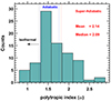 |
Fig. 2. Distribution of the polytropic index (α) for 82 ICME MOs. The data points to the left of the vertical dashed black line correspond to 12 isothermal MOs. The region between the vertical dashed blue line comprises 45 adiabatic MOs. Data points to the right of the vertical dashed red lines are the ICME MOs with super-adiabatic behaviour listed in Table B.1. The mean and median values are only for these 25 super-adiabatic ICME MOs. |
3.1. Heating and cooling processes
In a polytropic process, the ratio of pressure-volume work (δw) done by the system on the surroundings to the total heat transferred into the system (δq) is given as follows (e.g. Livadiotis 2018a, 2019a,b; Shaikh et al. 2023):
 (3)
(3)
where γ = 1 + 2/f is the adiabatic index. Equation (3) can also be written as follows (Livadiotis 2019b; Nicolaou et al. 2020; Shaikh et al. 2023):
 (4)
(4)
Figure 3 demonstrates the dependence of δq/δw on the effective number of degrees of freedom, f, for different values of α (Eq. (4)). For an expanding plasma, the red- (δq/δw > 0) and cyan-shaded (δq/δw < 0) regions correspond to plasma heating and cooling, respectively. In our study, we observe a mean value of α = 2.14. This high value suggests that the plasma within the ICME MOs behaves adiabatically only if f = 1.75. This is only possible if the plasma under examination has a strong anisotropic distribution or heterogeneous correlations among particle velocity components (see e.g. Livadiotis & Nicolaou 2021). Moreover, for f < 1.75, some physical processes should heat plasma protons within the ICME MO; in contrast, f > 1.75 corresponds to plasma cooling within expanding ICME MOs. It is well known that an ICME expands as it propagates in interplanetary space (Poomvises et al. 2010; Howard 2014). According to Jian et al. (2018), 71% of the ICMEs at 1 au are expanding. Therefore, an interesting possibility is that ICMEs consisting of particles with f = 3 expand super-adiabatically in interplanetary space. This leads to the conclusion that the expanding ICME MOs exhibit cooling phenomena. Furthermore, super-adiabatic heating and cooling are also observed for solar wind close to the Sun (α = 2.7; Nicolaou et al. 2020) and in Alfvénic solar wind at 1 au (α = 2.64; Shaikh et al. 2023). A thorough examination is necessary to identify the typical physical mechanisms contributing to plasma protons’ heating or cooling within ICME MOs.
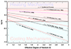 |
Fig. 3. Variation in |

De Avillez et al. (2018) find that hydrogen at high temperatures has an adiabatic index of γ = Cp/Cv = 5/3. We therefore assumed γ = 5/3 in Eq. (3), which is equivalent to setting f = 3 in Eq. (4), and examined the typical case of mono-atomic gas to determine the relationship between the change in internal energy and work/heat. Figure 4 shows the variation in δw/δq with respect to α for γ = 5/3. At α = 2.14, we have δw/δq = −1.41, suggesting that the work done by ICME MO plasma on its surroundings is 141% greater than the total heat supplied to it (see Appendix A for the case of other thermodynamics conditions). It appears that both the provided heat and some internal processes are contributing to the work being done (Shaikh et al. 2023). As a result, the examined super-adiabatic ICMEs’ MO plasma is cooling faster than adiabatically expected. If f = 3, the super-adiabatic result suggests an expanding plasma is cooling more than the adiabatic expectation and thus a super-cooling of the ICME MO plasma (heat emitted by the gas into the surrounding environment).
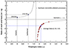 |
Fig. 4. Change in |

Coronal mass ejections dynamically evolve while propagating in the heliosphere, and several models have been developed to understand the origin and evolution of CMEs in interplanetary space (see e.g. Chen 1996, 2017; Riley et al. 2003; Webb & Howard 2012; Howard 2014, and references therein). Several models consider ICMEs with nearly isothermal or nearly adiabatic behaviour with 1 < α < 5/3 near their origin, with a specific evolution throughout their propagation in the heliosphere (Chen 1996; Riley et al. 2003). However, when employing such assumptions, the derived parameters (such as the temperature) are often underestimated or overestimated. The effect of the polytropic index (α) on the structural evolution is an open question, but the value of α has been observed to affect the energetics of CME (such as the temperature; see e.g. Chen 1996, 2017; Mishra et al. 2020). Moreover, CMEs also interact with, for example, the solar wind, high-speed streams, co-rotating interaction regions, and other CMEs. Thus, the morphology and kinematics of CMEs change, and we expect the energy of CMEs would also change. Our study helps address this discrepancy and allows us to better understand CME dynamics and energetics in the heliosphere (energy exchange with the surrounding solar wind). A further in-depth investigation is required to establish the characteristics of such super-adiabatic ICME MOs and the associated heating and cooling processes as they travel through the heliosphere.
4. Conclusion
The dynamic evolution, structural deformation, and heating and cooling of ICMEs are outstanding problems in solar physics (Savani et al. 2011; Lee et al. 2009; Murphy et al. 2011; Byrne et al. 2010; Liu et al. 2006; Shaikh & Raghav 2022). ICME plasma is believed to have either an adiabatic or isothermal nature in the heliosphere (e.g. Mishra & Wang 2018; Osherovich et al. 1993; Liu et al. 2006; Dayeh & Livadiotis 2022). We provide the first evidence that ICME MOs at 1 au can exhibit super-adiabatic properties (α ≳ 2 with f = 3). The super-adiabatic cooling process dominates in all 25 of the analysed ICME MOs. We also note that for an average α = 2.14, the ICME MOs show adiabatic processes only if f = 1.75. Interestingly, our results are consistent with the polytropic behaviour of the solar wind proton near the Sun (Nicolaou et al. 2020) and the Alfvénic region at 1 au (Shaikh et al. 2023). We argue that our results are extremely important for understanding the energy transfer from ICME MOs to surrounding plasma, such as the solar wind, planetary magnetosphere, and other large-scale structures (ICMEs, CIRs(corotating interaction regions), etc.). There are still several unresolved questions about the energetics of CMEs and ICMEs, including (1) which physical mechanisms are primarily responsible for the heating and cooling of ICME plasma, (2) what the driving mechanism is that changes the thermodynamic process from isothermal to super-adiabatic, (3) how uniform the heating and cooling is within a CME or ICME, and (4) how CME heating and cooling differ as a function of global CME parameters such as speed, mass, magnetic field strength, and configuration. In the future, we will try to answer some of these questions using multi-spacecraft data, combining measurements from Solar Orbiter and Parker Solar Probe.
Acknowledgments
We thank the ACE SWEPAM instrument team and the ACE Science Center for providing the ACE data. We acknowledge the use of NASA’s Goddard Space Flight Center (GSFC) Space Physics Data Facility’s Coordinated Data Analysis Web (CDAWeb) to provide access to the data utilised in this study. ZS thanks Ivan Vasko (UTD, TX) for fruitful discussion and valuable suggestions. Z.S. is supported by NASA grant No. 80NSSC20K1325 and 80NSSC23K0413. AR and OD are supported by the SERB project (CRG/2020/002314), while KG is supported by the DST-INSPIRE fellowship [IF210212].
References
- Akmal, A., Raymond, J. C., Vourlidas, A., et al. 2001, ApJ, 553, 922 [NASA ADS] [CrossRef] [Google Scholar]
- Bemporad, A., & Mancuso, S. 2010, ApJ, 720, 130 [NASA ADS] [CrossRef] [Google Scholar]
- Bothmer, V., & Daglis, I. A. 2007, Space Weather: Physics and Effects (Springer Science& Business Media) [CrossRef] [Google Scholar]
- Burlaga, L., Sittler, E., Mariani, F., & Schwenn, A. R., 1981, J. Geophys. Res.: Space Phys., 86, 6673 [NASA ADS] [CrossRef] [Google Scholar]
- Butler, S., Chen, W., & Turkakin, H. 2022, ApJ, 935, 164 [NASA ADS] [CrossRef] [Google Scholar]
- Byrne, J. P., Maloney, S. A., McAteer, R., Refojo, J. M., & Gallagher, P. T. 2010, Nat. Commun., 1, 1 [NASA ADS] [CrossRef] [Google Scholar]
- Chandrasekhar, S. 1933, MNRAS, 93, 390 [NASA ADS] [CrossRef] [Google Scholar]
- Chen, J. 1996, J. Geophys. Res.: Space Phys., 101, 27499 [NASA ADS] [CrossRef] [Google Scholar]
- Chen, P. 2011, Liv. Rev. Sol. Phys., 8, 1 [NASA ADS] [Google Scholar]
- Chen, J. 2017, Phys. Plasmas, 24, 9 [Google Scholar]
- Chen, J., & Garren, D. A. 1993, Geophys. Res. Lett., 20, 2319 [NASA ADS] [CrossRef] [Google Scholar]
- Chi, Y., Shen, C., Wang, Y., et al. 2016, Sol. Phys., 291, 2419 [Google Scholar]
- Ciaravella, A., & Raymond, J. 2008, ApJ, 686, 1372 [NASA ADS] [CrossRef] [Google Scholar]
- Dayeh, M. A., & Livadiotis, G. 2022, ApJ, 941, L26 [NASA ADS] [CrossRef] [Google Scholar]
- De Avillez, M. A., Anela, G. J., & Breitschwerdt, D. 2018, A&A, 616, A58 [NASA ADS] [CrossRef] [EDP Sciences] [Google Scholar]
- Fan, S., He, J., Yan, L., et al. 2018, Sol. Phys., 293, 1 [NASA ADS] [CrossRef] [Google Scholar]
- Farrugia, C. J., Osherovich, V., & Burlaga, L. 1995, J. Geophys. Res.: Space Phys., 100, 12293 [NASA ADS] [CrossRef] [Google Scholar]
- Forsyth, R., Bothmer, V., Cid, C., et al. 2006, Space Sci. Rev., 123, 383 [NASA ADS] [CrossRef] [Google Scholar]
- Ghag, K., Sathe, B., Raghav, A., et al. 2023, Universe, 9, 350 [NASA ADS] [CrossRef] [Google Scholar]
- Ghag, K., Pathare, P., Raghav, A., et al. 2024, Advances in Space Research, 73, 1064 [NASA ADS] [CrossRef] [Google Scholar]
- Gibson, S. E., & Low, B. 1998, ApJ, 493, 460 [NASA ADS] [CrossRef] [Google Scholar]
- Good, S., Hatakka, L., Ala-Lahti, M., et al. 2022, MNRAS, 514, 2425 [NASA ADS] [CrossRef] [Google Scholar]
- Gopalswamy, N. 2006, Space Sci. Rev., 124, 145 [Google Scholar]
- Gosling, J. 1999, J. Geophys. Res.: Space Phys., 104, 19851 [NASA ADS] [CrossRef] [Google Scholar]
- Gosling, J. 2012, Space Sci. Rev., 172, 187 [NASA ADS] [CrossRef] [Google Scholar]
- Gosling, J., Riley, P., & Skoug, R. 2001, J. Geophys. Res.: Space Phys., 106, 3709 [NASA ADS] [CrossRef] [Google Scholar]
- Howard, T. 2011, Coronal Mass Ejections: An Introduction (Springer Science& Business Media) [CrossRef] [Google Scholar]
- Howard, T. 2014, Space Weather and Coronal Mass Ejections (Springer) [CrossRef] [Google Scholar]
- Huang, Y.-M., Zweibel, E. G., & Sovinec, C. R. 2006, Phys. Plasmas, 13, 092102 [NASA ADS] [CrossRef] [Google Scholar]
- Jian, L., Russell, C., Luhmann, J., & Skoug, R. M. 2006, Sol. Phys., 239, 393 [NASA ADS] [CrossRef] [Google Scholar]
- Jian, L. K., Russell, C. T., Luhmann, J. G., & Galvin, A. B. 2018, ApJ, 855, 114 [Google Scholar]
- Klein, L., & Burlaga, L. 1982, J. Geophys. Res.: Space Phys., 87, 613 [NASA ADS] [CrossRef] [Google Scholar]
- Krall, J., Chen, J., & Santoro, R. 2000, ApJ, 539, 964 [NASA ADS] [CrossRef] [Google Scholar]
- Lee, J.-Y., Raymond, J., Ko, Y.-K., & Kim, K.-S. 2009, ApJ, 692, 1271 [NASA ADS] [CrossRef] [Google Scholar]
- Lepping, R., Jones, J., & Burlaga, L. 1990, J. Geophys. Res.: Space Phys., 95, 11957 [NASA ADS] [CrossRef] [Google Scholar]
- Li, H., Wang, C., Richardson, J. D., & Tu, C. 2017, ApJ, 851, L2 [NASA ADS] [CrossRef] [Google Scholar]
- Liu, Y., Richardson, J. D., & Belcher, J. W. 2005, Planet. Space Sci., 53, 3 [Google Scholar]
- Liu, Y., Richardson, J., Belcher, J., Kasper, J., & Elliott, H. 2006, J. Geophys. Res.: Space Phys., 111, A7 [Google Scholar]
- Livadiotis, G. 2018a, Entropy, 20, 799 [NASA ADS] [CrossRef] [Google Scholar]
- Livadiotis, G. 2018b, J. Geophys. Res.: Space Phys., 123, 1050 [NASA ADS] [CrossRef] [Google Scholar]
- Livadiotis, G. 2019a, ApJ, 874, 10 [CrossRef] [Google Scholar]
- Livadiotis, G. 2019b, Entropy, 21, 1041 [NASA ADS] [CrossRef] [Google Scholar]
- Livadiotis, G., & Nicolaou, G. 2021, ApJ, 909, 127 [NASA ADS] [CrossRef] [Google Scholar]
- Manchester, W. B., IV, Gombosi, T. I., Roussev, I., et al. 2004, J. Geophys. Res.: Space Phys., 109, A2 [Google Scholar]
- McComas, D., Gosling, J., Hammond, C., et al. 1994, Geophys. Res. Lett., 21, 1751 [NASA ADS] [CrossRef] [Google Scholar]
- McComas, D. J., Bame, S. J., Barker, P., et al. 1998, Space Sci. Rev., 86, 563 [CrossRef] [Google Scholar]
- Mei, Z., Shen, C., Wu, N., et al. 2012, MNRAS, 425, 2824 [NASA ADS] [CrossRef] [Google Scholar]
- Mishra, W., & Wang, Y. 2018, ApJ, 865, 50 [NASA ADS] [CrossRef] [Google Scholar]
- Mishra, W., Wang, Y., Teriaca, L., Zhang, J., & Chi, Y. 2020, Front. Astron. Space Sci., 7, 1 [NASA ADS] [CrossRef] [Google Scholar]
- Moldwin, M. 2022, An Introduction to Space Weather (Cambridge University Press) [CrossRef] [Google Scholar]
- Murphy, N. A., Raymond, J., & Korreck, K. 2011, ApJ, 735, 17 [NASA ADS] [CrossRef] [Google Scholar]
- Nicolaou, G., Livadiotis, G., & Moussas, X. 2014, Sol. Phys., 289, 1371 [NASA ADS] [CrossRef] [Google Scholar]
- Nicolaou, G., Livadiotis, G., & Wicks, R. T. 2019, Entropy, 21, 997 [NASA ADS] [CrossRef] [Google Scholar]
- Nicolaou, G., Livadiotis, G., Wicks, R. T., Verscharen, D., & Maruca, B. A. 2020, ApJ, 901, 26 [CrossRef] [Google Scholar]
- Nicolaou, G., Livadiotis, G., & McComas, D. J. 2023, ApJ, 948, 22 [CrossRef] [Google Scholar]
- Nieves-Chinchilla, T., Linton, M., Hidalgo, M. A., et al. 2016, ApJ, 823, 27 [NASA ADS] [CrossRef] [Google Scholar]
- Nieves-Chinchilla, T., Vourlidas, A., Raymond, J. C., et al. 2018, Sol. Phys., 293, 1 [NASA ADS] [CrossRef] [Google Scholar]
- Nieves-Chinchilla, T., Jian, L. K., Balmaceda, L., et al. 2019, Sol. Phys., 294, 89 [Google Scholar]
- Osherovich, V., Farrugia, C., Burlaga, L., et al. 1993, J. Geophys. Res.: Space Phys., 98, 15331 [NASA ADS] [CrossRef] [Google Scholar]
- Osherovich, V. A., Fainberg, J., Stone, R., Fitzenreiter, R., & Vinas, A. 1998, Geophys. Res. Lett., 25, 3003 [NASA ADS] [CrossRef] [Google Scholar]
- Osherovich, V. A., Fainberg, J., & Stone, R. 1999, Geophys. Res. Lett., 26, 401 [NASA ADS] [CrossRef] [Google Scholar]
- Owens, M. 2009, Sol. Phys., 260, 207 [NASA ADS] [CrossRef] [Google Scholar]
- Parker, E. 1965, Space Sci. Rev., 4, 666 [NASA ADS] [CrossRef] [Google Scholar]
- Poomvises, W., Zhang, J., & Olmedo, O. 2010, ApJ, 717, L159 [NASA ADS] [CrossRef] [Google Scholar]
- Pulkkinen, T. 2007, Liv. Rev. Sol. Phys., 4, 1 [Google Scholar]
- Raghav, A. N., & Shaikh, Z. I. 2020, MNRAS, 493, L16 [NASA ADS] [CrossRef] [Google Scholar]
- Raghav, A., Shaikh, Z., Vemareddy, P., et al. 2023, Sol. Phys., 298, 64 [NASA ADS] [CrossRef] [Google Scholar]
- Richardson, I. G., & Cane, H. V. 2010, Sol. Phys., 264, 189 [NASA ADS] [CrossRef] [Google Scholar]
- Richardson, I., & Cane, H. 2024, Near-Earth Interplanetary Coronal Mass Ejections Since January 1996 (Harvard Dataverse) [Google Scholar]
- Riley, P., Linker, J., Mikić, Z., et al. 2003, J. Geophys. Res.: Space Phys., 108, A7 [Google Scholar]
- Savani, N., Owens, M. J., Rouillard, A., et al. 2011, ApJ, 731, 109 [NASA ADS] [CrossRef] [Google Scholar]
- Schwenn, R. 2006, Liv. Rev. Sol. Phys., 3, 1 [NASA ADS] [Google Scholar]
- Shaikh, Z. I., & Raghav, A. N. 2022, ApJ, 938, 146 [NASA ADS] [CrossRef] [Google Scholar]
- Shaikh, Z. I., & Vichare, G. 2022, 2022 USRI-RCRS, 1 [Google Scholar]
- Shaikh, Z. I., Raghav, A. N., Vichare, G., Bhaskar, A., & Mishra, W. 2018, ApJ, 866, 118 [NASA ADS] [CrossRef] [Google Scholar]
- Shaikh, Z. I., Raghav, A. N., Vichare, G., Bhaskar, A., & Mishra, W. 2020, MNRAS, 494, 2498 [NASA ADS] [CrossRef] [Google Scholar]
- Shaikh, Z. I., Raghav, A. N., Vichare, G., D’Amicis, R., & Telloni, D. 2023, MNRAS, 519, L62 [Google Scholar]
- Sittler, E., Jr, & Burlaga, L. 1998, J. Geophys. Res.: Space Phys., 103, 17447 [NASA ADS] [CrossRef] [Google Scholar]
- Smith, C. W., L’Heureux, J., Ness, N. F., et al. 1998, Space Sci. Rev., 86, 613 [Google Scholar]
- Song, H. Q., Zhang, J., Cheng, X., et al. 2020, ApJ, 901, L21 [NASA ADS] [CrossRef] [Google Scholar]
- Song, H., Li, L., Sun, Y., et al. 2021, Sol. Phys., 296, 1 [NASA ADS] [CrossRef] [Google Scholar]
- Totten, T., Freeman, J., & Arya, S. 1995, J. Geophys. Res.: Space Phys., 100, 13 [NASA ADS] [CrossRef] [Google Scholar]
- Wang, C., Du, D., & Richardson, J. 2005, J. Geophys. Res.: Space Phys., 110, A10 [Google Scholar]
- Wang, J., Zhao, Y., Feng, H., et al. 2019, A&A, 632, A129 [NASA ADS] [CrossRef] [EDP Sciences] [Google Scholar]
- Webb, D. F., & Howard, T. A. 2012, Liv. Rev. Sol. Phys., 9, 1 [Google Scholar]
- Zurbuchen, T. H., & Richardson, I. G. 2006, Coronal Mass Ejections, Space Sciences Series of ISSI, (New York: Springer), 21, 31 [NASA ADS] [CrossRef] [Google Scholar]
Appendix A: Physical interpretation of distinct thermodynamic conditions
In the case of an isobaric process, α = 0, a δw/δq = 0.40 suggests that 40% of the total heat will be utilised to accomplish work, and the remaining will increase the internal energy (i.e. increase the temperature). Furthermore, for isothermal processes, α = 1, a δw/δq = 1 indicates that all heat introduced into the system is employed to perform work (i.e. compression at constant temperature). As a result, the system’s internal energy will not vary, meaning that the system’s temperature will remain constant. It is worth noting that when α = 5/3, the system enters an isentropic state, and we can witness a heating-to-cooling transition in the δw/δq ratio. Moreover, as α increases (and the system eventually is subject to an isochoric process), the work to supplied heat ratio decreases and is finally zero at α = ∞. For example, at α = 2.86, we have δw/δq = −0.56, which implies that the work done by ICME MO plasma on its surroundings represents 56% of the total heat. In contrast, the remaining 44% supplied total heat increases the internal energy of the ICME MO. If we increase the index further, for example to α = 10, the δw/δq = −0.08, suggesting δw → 0 as α → ∞. Thus, the system behaves in an isochoric fashion, indicating that no work will be performed and all the heat supplied into the system is used to increase the internal energy.
Appendix B: List of super-adiabatic ICME intervals
Here, we list the 25 ICME MO events that show super-adiabatic characteristics. Table B.1 summarises their average plasma properties and thermodynamic parameters, with detailed column descriptions included in the caption.
Super-adiabatic ICME MO intervals with average plasma parameters: IMF magnitude (Bmag), proton speed (Vp), temperature (Tp), density (Np), plasma beta (βp), and pressures (magnetic, Pmag, thermal, Pth, dynamic, Psw). The other columns show the thermodynamics parameters as described in the text. Note that f is calculated assuming the studied region is adiabatic. Ellipses (⋯) indicate an absence of data.
All Tables
Super-adiabatic ICME MO intervals with average plasma parameters: IMF magnitude (Bmag), proton speed (Vp), temperature (Tp), density (Np), plasma beta (βp), and pressures (magnetic, Pmag, thermal, Pth, dynamic, Psw). The other columns show the thermodynamics parameters as described in the text. Note that f is calculated assuming the studied region is adiabatic. Ellipses (⋯) indicate an absence of data.
All Figures
|
Fig. 1. ICME event observed by ACE from December 16 to December 17, 2006. Upper panel, from top to bottom: Temporal variation in the total IMF (the interplanetary magnetic field) BT, IMF vector Bvec = (Bx, By, Bz), azimuthal (ϕ = tan−1(By/Bx)) and elevation ( |
| In the text | |
|
Fig. 2. Distribution of the polytropic index (α) for 82 ICME MOs. The data points to the left of the vertical dashed black line correspond to 12 isothermal MOs. The region between the vertical dashed blue line comprises 45 adiabatic MOs. Data points to the right of the vertical dashed red lines are the ICME MOs with super-adiabatic behaviour listed in Table B.1. The mean and median values are only for these 25 super-adiabatic ICME MOs. |
| In the text | |
|
Fig. 3. Variation in |
| In the text | |
|
Fig. 4. Change in |
| In the text | |
Current usage metrics show cumulative count of Article Views (full-text article views including HTML views, PDF and ePub downloads, according to the available data) and Abstracts Views on Vision4Press platform.
Data correspond to usage on the plateform after 2015. The current usage metrics is available 48-96 hours after online publication and is updated daily on week days.
Initial download of the metrics may take a while.