| Issue |
A&A
Volume 691, November 2024
|
|
|---|---|---|
| Article Number | L11 | |
| Number of page(s) | 8 | |
| Section | Letters to the Editor | |
| DOI | https://doi.org/10.1051/0004-6361/202452168 | |
| Published online | 08 November 2024 | |
Letter to the Editor
Dependence of the polytropic behaviour of solar wind protons on temperature anisotropy and plasma β near L1
1
Department of Physics, National and Kapodistrian University of Athens, Athens, Greece
2
Department of Space and Climate Physics, Mullard Space Science Laboratory, University College London, Dorking, Surrey RH5 6NT, UK
3
Princeton University, Princeton, NJ 08544, USA
⋆ Corresponding author; This email address is being protected from spambots. You need JavaScript enabled to view it.
Received:
7
September
2024
Accepted:
11
October
2024
Abstract
Context. A polytropic process describes the transition of a fluid from one state to another through a specific relationship between the fluid density and temperature, while the value of the polytropic index that governs this relationship determines the heat transfer and the effective degrees of freedom of that specific process.
Aims. In this paper we investigate in depth the relationship between the proton effective polytropic index γ in the solar wind, the proton anisotropy α, and plasma β, while – for the first time to our knowledge to such an extent – we further investigate the dependence of the partial (with respect to the magnetic field) polytropic index to both the above-mentioned plasma parameters.
Methods. To this end we use the entire Wind dataset spanning the 1995 to 2023 time period to derive the distributions of the polytropic index in the near-Earth space (L1).
Results. Our results indicate that the proton γ increases with increasing proton anisotropy and decreases with increasing plasma β. Finally, we show that even though the average (over long time periods) total and partial proton polytropic index values are very close, these values correspond to isotropic plasma alone, with a further balance between the thermal and magnetic pressure.On the contrary, for shorter time periods and/or specific solar wind structures, where the proton anisotropy and plasma β exhibit deviations from these average values, the partial proton polytropic index exhibits significant variation that is dependent on the anisotropy and on plasma β.
Key words: plasmas / Sun: heliosphere / solar wind
© The Authors 2024
 Open Access article, published by EDP Sciences, under the terms of the Creative Commons Attribution License (https://creativecommons.org/licenses/by/4.0), which permits unrestricted use, distribution, and reproduction in any medium, provided the original work is properly cited.
This article is published in open access under the Subscribe to Open model. This email address is being protected from spambots. You need JavaScript enabled to view it. to support open access publication.
1. Introduction
Polytropic behaviour is a macroscopic relationship between plasma (and any fluid-like system in general) moments; in other words, density, n, versus pressure, P, or temperature, T, that describes the transition of a plasma from one state to another under constant specific heat (Parker 1963; Chandrasekhar 1957):
 (1)
(1)
Here the polytropic index γ is characteristic for individual plasma streamlines, and it may vary for different plasma species within different plasma regimes, thus indicating different thermodynamical states (Kartalev et al. 2006; Nicolaou et al. 2014a; Livadiotis 2016).
Through the polytropic equation we achieve a closure of the hierarchy of fluid equations, or between the higher order moments (such as temperature and pressure) of the velocity distribution function of plasma particles and plasma density (Kuhn et al. 2010). In addition, the polytropic relationship is directly related to plasma thermodynamics as it provides insight about the plasma heating and cooling and the effective dimensionality of the system without the necessity to solve the energy equation, which can be very complicated (Kartalev et al. 2006). Therefore, several studies analyse plasma observations and determine the polytropic index of different species throughout the heliosphere in order to reveal their thermodynamic properties. Relevant examples include, but are not limited to, the compression ratio of shocks (Parker 1961; Scherer et al. 2016; Livadiotis 2015; Nicolaou & Livadiotis 2017), planetary magnetospheres (Arridge et al. 2009; Nicolaou et al. 2014b; Dialynas et al. 2018; Park et al. 2019), solar wind periodic density structures (Katsavrias et al. 2024), interplanetary coronal mass ejections (Dayeh & Livadiotis 2022; Ghag et al. 2024), interplanetary space (Totten et al. 1995; Elliott et al. 2019; Abraham et al. 2022; Dakeyo et al. 2022), and the heliosheath (Livadiotis & McComas 2013). The value of γ characterizes specific processes in individual fluid parcels. Many space plasmas exhibit a positive correlation between their density and temperature (γ > 1), with their most frequent polytropic index close to the value of the adiabatic process (i.e. γ = 5/3) for three effective degrees of freedom (e.g. Nicolaou et al. 2014a; Livadiotis 2018). Adiabatic processes characterize plasma flows with nearly zero heat transition. However, this ideal adiabatic process can be disturbed from turbulent heating or wave generation, resulting in sub-adiabatic (1 < γ < 5/3) and super-adiabatic (5/3 < γ < ∞), respectively (Borovsky et al. 1998; Katsavrias et al. 2024).
Regardless of the specific process, space plasmas are in general described by anisotropic velocity distributions, which means that the perpendicular and parallel directions, with respect to the magnetic field, have different thermal properties (Desta et al. 2024). These are described with the temperature parameters of T⊥ and T∥, while their ratio defines the anisotropy as α = T⊥/T∥. This anisotropy determines the effective dimensionality of the velocity distribution, which is directly dependent on the polytropic index. In a recent study, Livadiotis & Nicolaou (2021) combined theoretical modelling with observational data from Wind during the first 73 days of 1995 to show that the lowest and classical value of the adiabatic polytropic index (i.e. γ = 5/3) occurs in the isotropic case, while higher values of the adiabatic index characterize more anisotropic plasmas.
In this paper we revisit the dependence of the polytropic index to plasma anisotropy using approximately three solar cycles worth of solar wind data from the Wind spacecraft. We further investigate the dependence of the polytropic index to plasma β, which quantifies the partitioning of energy density between the plasma pressure and the magnetic field pressure, and thus plays a vital role in the polarization of plasma fluctuations (Verscharen et al. 2019). Finally, we investigate for the first time to our knowledge to such an extent the dependence of the partial (with respect to the magnetic field) polytropic index to both the anisotropy and plasma β.
2. Data
We used solar wind measurements from the Solar Wind Experiment (SWE; Ogilvie et al. 1995) instrument on board the Wind spacecraft near L1 with ≈98 s resolution (the resolution varied over the course of the mission). We considered the solar wind proton number density (np) and the proton thermal speed elements of the temperature tensor (vth, ⊥ and vth, ∥) with their respective standard deviations, as well as the solar wind bulk speed. Finally, we obtained the solar wind magnetic field vector from the Magnetic Field Instrument (MFI; Lepping et al. 1995). Our dataset includes the entire Wind era (1995–2023). The scalar temperature (T) is derived from the thermal speed tensor assuming a gyro-tropic plasma as
 (2)
(2)
where T∥ = mpvth, ∥2/2kb and T⊥ = mpvth, ⊥2/2kb (with kb being the Boltzmann constant and mp the proton mass). Finally, the proton plasma β is derived as the ratio of energy density between the plasma thermal pressure (Pth = nkBT) to the magnetic field pressure (Pmag = B2/2μ0), where μ0 is the vacuum permeability. For the calculation of γ we follow the methodology introduced in Katsavrias et al. (2024) and is presented in detail in the appendix.
3. Results
3.1. Distribution of the polytropic index, anisotropy and plasma β during the entire Wind era
Figure 1a shows the histograms of the derived (filtered) polytropic index, anisotropy, and plasma β for the entire Wind dataset spanning the 1995–2023 time period. We note that there is a sharp dip in the histogram of the filtered values for γ ≈ 1, which corresponds to isothermal plasma. This is due to the filtering of the Pearson coefficient and the inverse polytropic index (see details in the Appendix). For these intervals, when one parameter varies significantly while the other is nearly constant, the regression process fails because it cannot determine a slope close to zero (for the forward regression) or close to infinity (for the inverse regression). This further means that even though the derived γs were derived using the best of fits, the filtering also excluded real near-isothermal values (see also Nicolaou et al. 2014a, and discussion therein).
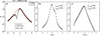 |
Fig. 1. Histograms and distributions for the entire Wind dataset spanning the 1995–2023 time period: (a) histogram of γ and best-fit κ-Gaussian distribution (solid red line), (b) histogram of anisotropy, and (c) histogram of plasma β. |
Therefore, in order to determine the average γ value of the distribution, we performed a weighted fitting focusing on its tails rather than its most frequent value. Following Livadiotis & McComas (2011) and Nicolaou et al. (2014a), we fitted a κ-Gaussian distribution given by
![Mathematical equation: $$ \begin{aligned} f(\gamma ,\overline{\gamma },\kappa _{0},\sigma ) \propto \left[ 1 + \frac{\left( \gamma - \overline{\gamma }\right)^{2}}{\kappa _{0}\cdot \sigma ^{2}} \right]^{-\kappa _{0}-3/2}. \end{aligned} $$](/articles/aa/full_html/2024/11/aa52168-24/aa52168-24-eq3.gif) (3)
(3)
The weighted κ-Gaussian fit in the case of the entire Wind dataset (solid red line in Fig. 1a) results in a  with σ ≈ 2.51. This is in agreement with the results of Katsavrias et al. (2024) and Livadiotis (2018), who estimated
  and ≈1.86, respectively. Furthermore, the anisotropy (Fig. 1b) is distributed with a mode near α ≈ 0.89 and a mean near α ≈ 0.83 (indicating a near-symmetric distribution), while plasma β values (Fig. 1c) are distributed with a mode near β ≈ 0.56 and a mean near β ≈ 0.43. We note that the anisotropy mode is quite close to the value derived by Livadiotis & Nicolaou (2021), even though these authors used only a small fraction of the Wind dataset (only 75 days during 1995).
Figure 2 shows the histograms of the partial filtered polytropic index in the perpendicular and parallel direction (with respect to the local magnetic field tensor), as well as the respective plasma β values. Interestingly, the γ⊥ distribution (Fig. 2a) exhibits very similar mean with the total polytropic index ( ) with a slightly increased σ ≈ 3.65. In contrast, the γ∥ distribution (Fig. 2b) exhibits a slightly increased mean (
 ) with a simultaneous broadening of the κ-Gaussian distribution by more than a factor of two (σ ≈ 7.27). Along the same lines, the perpendicular plasma β distribution exhibits very similar mode and mean with the total distribution, while the parallel plasma β distribution is less symmetric as it exhibits a mode near β∥ ≈ 0.71 and a mean near β∥ ≈ 0.47. Our results are qualitatively consistent with those by Nicolaou et al. (2021) in that the polytropic index exhibit similar values on average, regardless of the temperature tensor element used. Nevertheless, the latter authors used only one year of Wind data (2015) and derived partial polytropic indices distributions, which exhibited smaller mean values and σ values. Here, using the entire Wind dataset, we show that the σ of the parallel polytropic index distribution is much larger than that of the total and perpendicular polytropic index distribution. Since, this larger σ could be the reason for the ≈0.2 difference between the total and the parallel
  , further analysis is needed in order to conclude on the behaviour of the total and partial polytropic index. Finally, our result indicates a connection between plasma β and the polytropic index, which will be further investigated and discussed in the following sections.
3.2. The αβγ interrelationship
In Fig. 3 we show the 2D histograms of (from left to right) γ and log10(α), log10(β) and log10(α), and γ and log10(β) for the entire Wind data. We note that the α and β values were also calculated as the mean over each 10 min sub-interval to match the time resolution of the derived γ. In all panels the white solid line shows the most frequent value (mode) of the variable in the y-axis as a function of the variable in the x-axis, while the logarithm of occurrence in each bin is colour-coded. During the analysed time period, log10(α) ranges from ≈–0.5 to 0.5 for γ in the [1 3] range (left panel of Fig. 3). Moreover, the white solid line shows the mode of γ at each log10(α) bin. We note that we did not perform the k-Gaussian fitting here, but rather simply estimated the most probable value at each log10(α) bin. Finally, the magenta dashed line corresponds to the predicted γ values using the theoretical model of Livadiotis & Nicolaou (2021) given by
 (4)
(4)
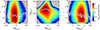 |
Fig. 3. Two-dimensional histograms of the αβγ interrelationship. Left panel: Two-dimensional histogram of γ and log10(α). The white solid line shows the most frequent value of γ in each log10(α), while the magenta dashed line shows the predicted γ using the theoretical model of Livadiotis & Nicolaou (2021). Middle panel: Two-dimensional histogram of log10(β) and log10(α). The white solid line shows the most frequent value of log10(β) in each log10(α), while the magenta dashed line shows the predicted log10(β) using the function: log10β = log10β0 + λ ⋅ |log10α−log10α0|δ. Right panel: Two-dimensional histogram of γ and log10(β). The white solid line shows the most frequent value of γ in each log10(β), while the magenta dashed line shows the predicted γ using a non-linear fitting by substituting the previous function to the theoretical model of Livadiotis & Nicolaou (2021). In all panels the logarithm of occurrence in each bin is colour-coded in red corresponding to 10 000 values. |
As shown, there is a good agreement between the theoretical model and the most frequent γ with an overall Pearson R = 0.67 and RMSE = 0.16. The variation in the most frequent γ value with respect to anisotropy is ≈12% for log10(α) in the [–0.3 0.2] range, while it becomes much larger for higher or lower log10(α). This is probably attributed to the sample statistics as the occurrence for this range falls below 1000 points per bin. Furthermore, both the model and observations indicate that γ converges to the adiabatic value (i.e. 1.67) near the isotropic case, while it increases to super-adiabatic values as the anisotropy increases or decreases.
The middle panel of Fig. 3 shows the 2D histogram log10(β) and log10(α), the well-known ‘Brazil plot’ (Verscharen et al. 2019). Once again, the white solid line shows the mode of log10(β) at each log10(α) bin. As shown, the isotropic case corresponds to β values close to 1 (i.e. the case of balance between the thermal and magnetic pressure). On the other hand, as we move away from isotropy, there is an almost symmetric decrease in plasma β, which indicates that the magnetic pressure becomes more important than the thermal pressure by approximately a factor of 5. We further determined the relationship between the modes of log10(β) at each log10(α) bin by fitting the function
 (5)
(5)
where the free parameters β0 = −0.1, α0 = 0.133, λ = −0.66, and δ = 0.86 were estimated using a least-squares approach. Moreover, the modelled β versus the actual β mode exhibit a Pearson R = 0.97 and RMSE = 0.03.
Finally, the right panel of Fig. 3 shows the 2D histogram γ and log10(β). As shown, log10(β) ranges from ≈–1.3 to 0.5 for γ in the [1 3] range, while the white solid line shows the mode of γ at each log10(β) bin. There is a clear anti-correlation between γ and log10(β), except at the very low log10(β) values (below –1.2), which (once again) correspond to bins with very low occurrence and the mode seems to be flattened. In order to determine the relationship between γ and log10(β), we combine the theoretical model of Livadiotis & Nicolaou (2021) given in Eq. (4) with the fitted function between log10(β) and log10(α) in Eq. (5). Solving the latter with respect to α,
![Mathematical equation: $$ \begin{aligned} \alpha =\alpha _0 \cdot 10^{\left[\frac{1}{\lambda }\cdot \log _{10}\left(\frac{\beta }{\beta _0}\right) \right]^\frac{1}{\delta }}, \end{aligned} $$](/articles/aa/full_html/2024/11/aa52168-24/aa52168-24-eq11.gif) (6)
(6)
and substituting in Eq. (4), we derive the polytropic index as a function of log10(β), which is shown with the magenta dashed line in the right panel of Fig. 3. The fitted function exhibits a very good agreement with observations with an overall Pearson R = 0.72 and RMSE = 0.135.
3.3. Dependence of the partial polytropic index to anisotropy, plasma β and solar wind speed
In order to further investigate the dependence of the partial polytropic index to anisotropy and plasma β, we first performed a binning of the index values with respect to latter parameters using bins of δα = δβ = 0.1. Then, from the values in each bin we derived the  ,
,  , and
, and  by fitting a κ-Gaussian distribution. We note that we accept a fitting only under the following conditions: (a) if the Pearson R between the γ histogram values and the κ-Gaussian fitting is higher than 0.95, (b) if the corresponding RMSE is lower than 0.1 and (c) if there are more than 1000 valid data points in each bin. The results are shown in Fig. 4.
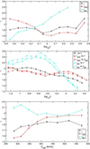 |
Fig. 4. Dependence of the partial polytropic index to anisotropy, plasma β and solar wind speed. Top panel: |


In detail, the dependence of  ,
,  , and
, and  on log10(α) is shown in the top panel of Fig. 4 with the black, red, and cyan solid lines, respectively. As shown, the behaviour of the
  exhibits similarities to the results shown in the previous section: it is close to the adiabatic value for the isotropic case, while it increases in the [1.8 1.9] range as the anisotropy reaches higher or lower values. On the contrary, the partial polytropic index exhibits completely different behaviour in the parallel and perpendicular direction. The
  is also close to the adiabatic value for the isotropic case; moreover, it exhibits higher values (compared to the total
  ) for decreasing anisotropy and lower values (closer to the adiabatic limit) for increasing anisotropy. On the other hand, the
  exhibits a monotonically increasing behaviour with respect to log10(α), spanning γ values in the [1.5 2.6] range.
We note that the anisotropy is defined as the ratio of the perpendicular to the parallel temperature components, and therefore the high α values (α > 1) correspond to distributions with their thermal speed being dominant in the perpendicular direction (with respect to the magnetic field), while the low α values (α < 1) correspond to distributions with their thermal speed being dominant in the parallel direction. Thus said, for α > 1, all the information can be found in the perpendicular direction, and even though the space dimensionality is decreased from 3D to 2D, the effective degrees of freedom are increased, which consequently leads to a decrease in  . To the same extent, the effective degrees of freedom in the parallel direction are decreased, which consequently leads to an increase in
  . The exact opposite behaviour occurs for α < 1.
The dependence of  ,
,  , and
, and  on log10(β) is shown in the middle panel of Fig. 4 with the black, red, and cyan solid lines, respectively. The
  exhibits a linear anti-correlation with log10(β), similar to the mode γ used in Fig. 3, while it exhibits a good agreement with the predicted γ using the simple linear fitting. This anti-correlation is in good agreement with the results of Nicolaou et al. (2020) who used Parker Solar Probe data during April 2–4, 2019, and showed a negative correlation between γ and plasma β. Furthermore, it is very close to the adiabatic value (see e.g. Livadiotis 2016) at the case of balance between the thermal and magnetic pressure density (β = 1). Once again, the partial polytropic index exhibits completely different behaviour in the parallel and perpendicular direction. The
  exhibits a similar anti-correlation as the total
  , while it reaches slightly decreased values (compared with total
  ) for log10(β < −0.4) and slightly increased values for log10(β > −0.4). This is in agreement with the results of Fig. 3 as β values lower than 1 are accompanied by higher anisotropy (e.g. the case of high-speed streams from coronal holes). On the other hand,
  exhibits significantly increased values (up to 2.6) for log10(β < −0.3) and a linear monotonically decrease for higher log10(β), reaching down to ≈1.3. We note that there is no significant difference if we use β∥ or β⊥ (dashed cyan and red lines, respectively) instead of the total β.
Finally, the dependence of  ,
,  , and
, and  on solar wind speed is shown in the bottom panel of Fig. 4. The total
  shows no clear dependence on solar wind speed, and furthermore fluctuates around ≈1.8, which is the
  of the entire Wind dataset (Fig. 1). This result is in agreement with Livadiotis (2018), who estimated an all-year weighted mean at 1.86, and further indicated that the polytropic index has no reason to exhibit a significant (average) variation (i.e. the same thermodynamic processes characterize the solar wind plasma). Any possible fluctuations of the solar wind bulk parameters will generally affect the entropy rather than the polytropic index estimations, because the latter is derived from the differences of those parameters. To the same extent, the
  and
and  also exhibit small fluctuations for VSW > 380 km/s. On the contrary, for VSW < 380 km/s,
  decreases from an average value of ≈1.9 to ≈1.6, while
  increases from an average value of ≈2 to ≈2.15. A possible explanation could be that these very low-speed protons have different thermodynamic properties compared to the average solar wind. Nevertheless, such low speed values are very close to the lower limit of Wind/SWE instrument, which may introduce significant uncertainty to the derivation of the proton velocity distribution. On the other hand, and although erroneous measurements may exist for low solar wind speeds, the bimodal behaviour of solar wind may contribute at some level (Dayeh et al. 2012).
4. Discussion and conclusions
We used the entire Wind dataset (approximately three solar cycles), spanning the time period 1995–2023, to investigate the dependence of the proton effective polytropic index to temperature anisotropy (α) and plasma β, as well as the behaviour of the partial proton polytropic index near L1. Our results show that on average, and over a long time period, one can derive similar (within ≈0.2) polytropic index values regardless of the temperature tensor element used. This result is in agreement with Nicolaou et al. (2021), who indicated that the anisotropic heating within the analysed streamlines is not significant enough to prevent accurately calculating the average polytropic index of the solar wind plasma protons. We emphasize that even though we did not require a constant anisotropy at each analysed window, we argue that a varying anisotropy would lead to significant deviations from the power law (Eq. (A.1)), which in turn would lead to deviations between the normal and inverse spectrum slope as well as to a decreased Pearson R. Thus, streamlines with varying anisotropy would be rejected by our filtering criteria.
On the other hand, even though the average total and partial polytropic index values are very close (i.e.  and
and  ), these values correspond to isotropic plasma (α ≈ 1), which is simultaneously accompanied by a balance between thermal and magnetic pressure (β ≈ 1). For shorter time periods and/or specific solar wind structures, where the anisotropy and plasma β exhibit deviations from these average values, γ and partial γ do exhibit variation and are further physically dependent on both α and β. Our results indicate that
  is generally closer to the total
  , especially during periods with highly anisotropic solar wind (α > 1) and low plasma β values (β < 1). This means that solar wind structures that exhibit such characteristics can be adequately described (in terms of thermodynamics) using the variations in the thermal speed only in the perpendicular direction.
The polytropic index also exhibits an anti-correlation with plasma β. We derived γ as a function of log10β by exploiting the theoretical model of Livadiotis & Nicolaou (2021) and the interrelationship between plasma β and proton anisotropy. This anti-correlation could originate from the increase in the effective degrees of freedom with increasing β and/or heating processes since higher proton β corresponds to increased proton thermal pressure. Similarly, for β < 1, when strong magnetic fields dominate the particle thermal motions, the thermodynamic processes are confined along the direction of the magnetic field, and thus the effective degrees of freedom are reduced, and/or there is a mechanism that effectively absorbs energy from the plasma protons. Nevertheless, according to Fig. 3, higher plasma β values correspond to nearly isotropic protons. This indicates that the effective degrees of freedom are approximately stable and heating is more likely to produce the decrease of the total γ.
It is finally worth mentioning that the plasma β and the proton temperature anisotropy exhibit a strong correlation with the sunspot number (Rz) and solar wind bulk speed (Vsw), respectively (see also Figs. B.1 and B.2). In detail, the Pearson R between β and Rz and between α and Vsw are –0.87 and 0.85, respectively. Nevertheless, γ exhibits poor correlations with both Rz and Vsw (right panels in Fig. B.2). Desta et al. (2024) investigated the theoretical relation between the polytropic index and anisotropic temperature, magnetic field, and flow speed in the context of the double-adiabatic Chew–Goldberger–Low (CGL) theory and Ulysses data. They found that the polytropic index exhibited variation depending on the magnetic field, flow speed, and anisotropic temperature, which may also exhibit a solar cycle dependence. In this work we have shown that γ is actually dependent on a non-linear combination of α and β, while both of these parameters describe complex processes in the solar wind plasma in contrast with the simple solar and solar wind parameters.
Finally, we emphasize that our study focuses on solar wind protons only at 1 AU. Nevertheless, the study of the polytropic behaviour in space and astrophysical plasmas leads to important knowledge about the velocity distribution functions of the plasma particles and the potential energy acting on them. Therefore, future studies of the behaviour of the total and partial polytropic of solar wind electrons, or even other ion species through the heliosphere will be of great interest.
Acknowledgments
The authors thank the National Space Science Data Center of the Goddard Space Flight Center for the use permission of Wind data and the NASA CDAWeb team for making these data available (http://cdaweb.gsfc.nasa.gov/istp_public/).
References
- Abraham, J. B., Verscharen, D., Wicks, R. T., et al. 2022, ApJ, 941, 145 [NASA ADS] [CrossRef] [Google Scholar]
- Arridge, C., McAndrews, H., Jackman, C., et al. 2009, Planet. Space Sci., 57, 2032 [NASA ADS] [CrossRef] [Google Scholar]
- Borovsky, J. E., Thomsen, M. F., Elphic, R. C., Cayton, T. E., & McComas, D.~J. 1998, J. Geophys. Res., 103, 20297 [NASA ADS] [CrossRef] [Google Scholar]
- Chandrasekhar, S. 1957, in An Introduction to the Study of Stellar Structure, (Dover Publications), Astrophysical monographs [Google Scholar]
- Dakeyo, J.-B., Maksimovic, M., Démoulin, P., Halekas, J., & Stevens, M. L. 2022, ApJ, 940, 130 [NASA ADS] [CrossRef] [Google Scholar]
- Dayeh, M. A., & Livadiotis, G. 2022, ApJ, 941, L26 [NASA ADS] [CrossRef] [Google Scholar]
- Dayeh, M. A., McComas, D. J., Allegrini, F., et al. 2012, ApJ, 749, 50 [NASA ADS] [CrossRef] [Google Scholar]
- Desta, E. T., Strauss, R. D., & Engelbrecht, N. E. 2024, ApJ, 966, 142 [NASA ADS] [CrossRef] [Google Scholar]
- Dialynas, K., Roussos, E., Regoli, L., et al. 2018, J. Geophys. Res., 123, 8066 [NASA ADS] [CrossRef] [Google Scholar]
- Elliott, H. A., McComas, D. J., Zirnstein, E. J., et al. 2019, ApJ, 885, 156 [Google Scholar]
- Ghag, K., Pathare, P., Raghav, A., et al. 2024, Adv. Space Res., 73, 1064 [NASA ADS] [CrossRef] [Google Scholar]
- Kartalev, M., Dryer, M., Grigorov, K., & Stoimenova, E. 2006, J. Geophys. Res., 111, A10107 [NASA ADS] [Google Scholar]
- Katsavrias, C., Nicolaou, G., Di Matteo, S., et al. 2024, A&A, 686, L10 [NASA ADS] [CrossRef] [EDP Sciences] [Google Scholar]
- Kuhn, S., Kamran, M., Jelic, N., et al. 2010, AIP Conf. Proc., 1306, 216 [NASA ADS] [CrossRef] [Google Scholar]
- Lepping, R. P., Acũna, M. H., Burlaga, L. F., et al. 1995, Space Sci. Rev., 71, 207 [Google Scholar]
- Livadiotis, G. 2015, ApJ, 809, 111 [NASA ADS] [CrossRef] [Google Scholar]
- Livadiotis, G. 2016, ApJS, 223, 13 [NASA ADS] [CrossRef] [Google Scholar]
- Livadiotis, G. 2018, Entropy, 20, 799 [NASA ADS] [CrossRef] [Google Scholar]
- Livadiotis, G. 2019, Stats, 2, 416 [CrossRef] [Google Scholar]
- Livadiotis, G., & McComas, D. J. 2011, ApJ, 741, 88 [NASA ADS] [CrossRef] [Google Scholar]
- Livadiotis, G., & McComas, D. J. 2013, J. Geophys. Res., 118, 2863 [NASA ADS] [CrossRef] [Google Scholar]
- Livadiotis, G., & Nicolaou, G. 2021, ApJ, 909, 127 [NASA ADS] [CrossRef] [Google Scholar]
- Newbury, J. A., Russell, C. T., & Lindsay, G. M. 1997, Geophys. Res. Lett., 24, 1431 [NASA ADS] [CrossRef] [Google Scholar]
- Nicolaou, G., & Livadiotis, G. 2017, ApJ, 838, 7 [NASA ADS] [CrossRef] [Google Scholar]
- Nicolaou, G., & Livadiotis, G. 2019, ApJ, 884, 52 [NASA ADS] [CrossRef] [Google Scholar]
- Nicolaou, G., Livadiotis, G., & Moussas, X. 2014a, Sol. Phys., 289, 1371 [NASA ADS] [CrossRef] [Google Scholar]
- Nicolaou, G., McComas, D. J., Bagenal, F., & Elliott, H. A. 2014b, J. Geophys. Res., 119, 3463 [NASA ADS] [CrossRef] [Google Scholar]
- Nicolaou, G., Livadiotis, G., & Wicks, R. T. 2019, Entropy, 21, 997 [NASA ADS] [CrossRef] [Google Scholar]
- Nicolaou, G., Livadiotis, G., Wicks, R. T., Verscharen, D., & Maruca, B. A. 2020, ApJ, 901, 26 [CrossRef] [Google Scholar]
- Nicolaou, G., Livadiotis, G., & Desai, M. I. 2021, Appl. Sci., 11, 4019 [NASA ADS] [CrossRef] [Google Scholar]
- Ogilvie, K. W., Chornay, D. J., Fritzenreiter, R. J., et al. 1995, Space Sci. Rev., 71, 55 [Google Scholar]
- Park, J., Shue, J., Nariyuki, Y., & Kartalev, M. 2019, J. Geophys. Res., 124, 1866 [NASA ADS] [CrossRef] [Google Scholar]
- Parker, E. N. 1961, ApJ, 134, 20 [NASA ADS] [CrossRef] [Google Scholar]
- Parker, E. 1963, in Interplanetary Dynamical Processes, (Interscience Publishers), Interscience monographs and texts in physics and astronomy [Google Scholar]
- Scherer, K., Fichtner, H., Fahr, H. J., Röken, C., & Kleimann, J. 2016, ApJ, 833, 38 [NASA ADS] [CrossRef] [Google Scholar]
- Siegel, A. F. 1982, Biometrika, 69, 242 [NASA ADS] [CrossRef] [Google Scholar]
- Totten, T. L., Freeman, J. W., & Arya, S. 1995, J. Geophys. Res., 100, 13 [Google Scholar]
- Verscharen, D., Klein, K. G., & Maruca, B. A. 2019, Living Rev. Sol. Phys., 16, 5 [NASA ADS] [Google Scholar]
Appendix A: Derivation of the polytropic index
For the calculation of γ we follow the methodology introduced in Katsavrias et al. (2024). We first need to analyse sufficiently short sub-intervals in order to minimize the possibility of mixing measurements of different streamlines (Kartalev et al. 2006; Livadiotis 2018; Nicolaou & Livadiotis 2019). In order to increase our statistics, we up-sample Wind data to 49 sec (half of the nominal resolution to avoid potential artifacts) using linear interpolation. Then, we use a sliding window of ≈10 min, which corresponds to 12 points per moving window, requiring that each window contains at least 9 valid points.
The next step is to perform a repeated median regression (Siegel 1982), which is a variation of the Theil–Sen estimator, to the logarithm of Eq. 1 for solar wind protons:
 (A.1)
(A.1)
In detail, for each sample point (ni, Ti), the median mi of the slopes (Tj − Ti)/(nj − ni), for i≠j, of lines through that point is derived. Then, the overall estimator is the median of these medians. We have used the repeated median regression over the more common least-squares linear fit as it offers a more robust option for our purposes. Given the small number of data points per window (up to 12 points), on which the fits are performed, even a singular outlier can detrimentally impact a least-squares fit, while the median regression is much less sensitive to outliers. It thus is optimal in evaluating γ. We further note that the estimation of γ by fitting in lnT versus lnn is much more straightforward, since it is based in directly measured quantities (Newbury et al. 1997; Kartalev et al. 2006). In contrast, fitting in lnP versus lnn would result in artifacts (biased correlations due to the fact that P is constructed from the measured n, thus not independently measured) and, furthermore, the error propagation would result in significantly higher uncertainty.
The next step is to filter our derived γ values using the following criteria. First, we examine the stability of Bernoulli’s integral in each window by requiring the standard deviation over the mean to be less than 2%. This condition is particularly important, as it enhances the possibility that the analysed sub-intervals correspond to individual streamlines, where the polytropic relation is valid (Kartalev et al. 2006). For the plasma near 1 AU, Bernoulli’s integral can be estimated from the Wind parameters following Livadiotis (2016):
 (A.2)
(A.2)
 (A.3)
(A.3)
Here VSW is the solar wind bulk speed, ρ is the proton mass density, and B is the interplanetary magnetic field strength, while γ is the total polytropic index. The second filter is the Pearson correlation coefficient of the regressed versus the measured data points, which we require to be higher than 0.8. The third, and final, filter is the special polytropic index (vinv), which corresponds to the inverse spectrum regression (see also Nicolaou et al. 2019; Livadiotis 2019), and must differ no more than 0.1:
 (A.4)
(A.4)
Examples of valid and invalid regressions are given in Fig. A.1.
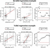 |
Fig. A.1. Example of an invalid (top panels) and valid (bottom panels) derivation of γ satisfying all the criteria set for this study. The left and middle panels show the cross plots of ln(Tp) vs. ln(np) and ln(np) vs. ln(Tp), respectively, with the Wind data shown as black circles (and the corresponding standard deviation with error bars) and the regressed values as the solid red lines. The right panels show Bernoulli’s integral estimate for the same window (black circles) along with the 2% limit (dashed red lines). |
A similar procedure is followed for the determination of γ⊥ and γ∥ simply by substituting temperature in Eq. A.1 with T⊥ and T∥, respectively. Finally, in order to match the time resolution of the derived γ’s, we also derive the average anisotropy and plasma β values as well as solar wind bulk speed over each 10 minutes sub-interval.
Appendix B: Supplementary figures
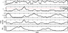 |
Fig. B.1. Time series (from top to bottom) of the total proton polytropic index (γ), the proton temperature anisotropy (α), plasma β, solar wind bulk speed and sunspot number (Rz). Each data point has been derived using a moving window of 365 days with a step of 10 days. Solar wind parameters and sunspot number correspond to the mean value in each moving window, while γ values correspond to the κ-Gaussian mean in each moving window. |
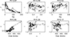 |
Fig. B.2. Same as Fig. B.1, but for the cross-plots between the total proton polytropic index (γ), the proton temperature anisotropy (α), plasma β, solar wind bulk speed, and sunspot number (Rz). |
All Figures
|
Fig. 1. Histograms and distributions for the entire Wind dataset spanning the 1995–2023 time period: (a) histogram of γ and best-fit κ-Gaussian distribution (solid red line), (b) histogram of anisotropy, and (c) histogram of plasma β. |
| In the text | |
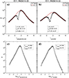 |
Fig. 2. Same as Fig. 1, but for: (a) γ⊥, (b) γ∥, (c) β⊥, and (d) β∥. |
| In the text | |
|
Fig. 3. Two-dimensional histograms of the αβγ interrelationship. Left panel: Two-dimensional histogram of γ and log10(α). The white solid line shows the most frequent value of γ in each log10(α), while the magenta dashed line shows the predicted γ using the theoretical model of Livadiotis & Nicolaou (2021). Middle panel: Two-dimensional histogram of log10(β) and log10(α). The white solid line shows the most frequent value of log10(β) in each log10(α), while the magenta dashed line shows the predicted log10(β) using the function: log10β = log10β0 + λ ⋅ |log10α−log10α0|δ. Right panel: Two-dimensional histogram of γ and log10(β). The white solid line shows the most frequent value of γ in each log10(β), while the magenta dashed line shows the predicted γ using a non-linear fitting by substituting the previous function to the theoretical model of Livadiotis & Nicolaou (2021). In all panels the logarithm of occurrence in each bin is colour-coded in red corresponding to 10 000 values. |
| In the text | |
|
Fig. 4. Dependence of the partial polytropic index to anisotropy, plasma β and solar wind speed. Top panel: |
| In the text | |
|
Fig. A.1. Example of an invalid (top panels) and valid (bottom panels) derivation of γ satisfying all the criteria set for this study. The left and middle panels show the cross plots of ln(Tp) vs. ln(np) and ln(np) vs. ln(Tp), respectively, with the Wind data shown as black circles (and the corresponding standard deviation with error bars) and the regressed values as the solid red lines. The right panels show Bernoulli’s integral estimate for the same window (black circles) along with the 2% limit (dashed red lines). |
| In the text | |
|
Fig. B.1. Time series (from top to bottom) of the total proton polytropic index (γ), the proton temperature anisotropy (α), plasma β, solar wind bulk speed and sunspot number (Rz). Each data point has been derived using a moving window of 365 days with a step of 10 days. Solar wind parameters and sunspot number correspond to the mean value in each moving window, while γ values correspond to the κ-Gaussian mean in each moving window. |
| In the text | |
|
Fig. B.2. Same as Fig. B.1, but for the cross-plots between the total proton polytropic index (γ), the proton temperature anisotropy (α), plasma β, solar wind bulk speed, and sunspot number (Rz). |
| In the text | |
Current usage metrics show cumulative count of Article Views (full-text article views including HTML views, PDF and ePub downloads, according to the available data) and Abstracts Views on Vision4Press platform.
Data correspond to usage on the plateform after 2015. The current usage metrics is available 48-96 hours after online publication and is updated daily on week days.
Initial download of the metrics may take a while.