| Issue |
A&A
Volume 695, March 2025
|
|
|---|---|---|
| Article Number | A146 | |
| Number of page(s) | 11 | |
| Section | The Sun and the Heliosphere | |
| DOI | https://doi.org/10.1051/0004-6361/202452984 | |
| Published online | 14 March 2025 | |
The Polytropic Index of Interplanetary Coronal Mass Ejections near L1
1
Department of Physics, National and Kapodistrian University of Athens, Athens, Greece
2
Department of Space and Climate Physics, Mullard Space Science Laboratory, University College London, Dorking, Surrey RH5 6NT, UK
3
Princeton University, Princeton, NJ 08544, USA
4
Applied Physics Laboratory, Johns Hopkins University, Laurel, MD, USA
5
NASA Goddard Space Flight Center, Greenbelt, MD, USA
6
Space Applications and Research Consultancy (SPARC), Athens, Greece
⋆ Corresponding author; This email address is being protected from spambots. You need JavaScript enabled to view it.
Received:
13
November
2024
Accepted:
14
February
2025
Abstract
Context. A polytropic process describes the transition of a fluid from one state to another through a specific relationship between the fluid density and temperature, and the value of the polytropic index that governs this relationship determines the heat transfer and the effective degrees of freedom of this specific process.Aims. In this paper, we investigate in depth the proton polytropic behaviour in interplanetary coronal mass ejections (ICMEs). Moreover, for the first time (to our knowledge and at such an extent) we further investigate the behaviour of both the total and partial polytropic indices within ICMEs with various magnetic field configurations inside the magnetic obstacles.Methods. To that end we used a list of 401 ICMEs identified from Wind measurements during more than two solar cycles (1995–2001), during which we derived the distributions of the polytropic index in the near-Earth space (L1).Results. Our results show that sheaths are sub-adiabatic, indicating turbulent plasma, while the value of γ further depends on the existence of a shock. Furthermore, the polytropic behaviour of the protons inside the ICME magnetic obstacles is dependent on the magnetic field configuration, with flux ropes with rotation above 90 deg exhibiting sub-adiabatic γ, while ejecta with no clear rotation exhibiting super-adiabatic γ, supporting the scenario that changes during the interplanetary evolution might affect the magnetic field configuration inside the magnetic obstacle.
Key words: Sun: heliosphere / solar wind
© The Authors 2025
 Open Access article, published by EDP Sciences, under the terms of the Creative Commons Attribution License (https://creativecommons.org/licenses/by/4.0), which permits unrestricted use, distribution, and reproduction in any medium, provided the original work is properly cited.
This article is published in open access under the Subscribe to Open model. This email address is being protected from spambots. You need JavaScript enabled to view it. to support open access publication.
1. Introduction
Coronal mass ejections (CMEs) are eruptions of magnetised plasma from the solar corona into the heliosphere. Their interplanetary signatures, so-called interplanetary coronal mass ejections (ICMEs), are typically comprise three major parts: (i) the shock; (ii) the sheath, a region of compressed and heated solar wind plasma; and (iii) the magnetic obstacle (MO), where the field vector smoothly rotates up to 180° (Zurbuchen & Richardson 2006). In the best cases, MOs are well-ordered magnetic clouds (single flux ropes). For example, in the case of a monotonic 180° magnetic field rotation, an MO could consist of a single flux rope. However, in the case of a rotation greater than 180° or more than one rotation, the MO could be considered as multiple flux ropes or spheromaks (Nieves-Chinchilla et al. 2018).
In space weather studies, ICMEs have paramount importance, as they lead to intense space weather consequences (Kilpua et al. 2015; Daglis et al. 2019). They are one of the main drivers of both geomagnetic activity (Borovsky & Denton 2006; Katsavrias et al. 2016) and outer radiation belt variability, as they can lead to the acceleration of multi-MeV energies (Katsavrias et al. 2015a; Turner et al. 2019) and to intense relativistic electron flux dropouts (Turner et al. 2012; Katsavrias et al. 2015b). Furthermore, ICME-driven shocks can produce solar energetic particle (SEP) events and their proton component solar proton events (SPEs), which are some of the most hazardous phenomena in space weather since they can present dangers to the increasingly complex electronics on board spacecraft and humans through extreme exposure, such as during extravehicular activities or from accumulated exposure over the course of a mission (Aminalragia-Giamini et al. 2020). Therefore, understanding ICME propagation and internal processes is an important aspect to further advance our space weather capabilities.
Thermodynamic properties of ICMEs can be studied using a polytropic state estimation. The polytropic behaviour is a macroscopic relationship between plasma (and any fluid-like system in general) moments (i.e., density, n, versus pressure, P, or temperature, T) that describes the transition of a plasma from one state to another under constant specific heat (Parker 1963; Chandrasekhar 1957):
 (1)
(1)
Here, the polytropic index γ is characteristic for individual plasma streamlines, and it may vary for different plasma species within different plasma regimes and thus indicate different thermodynamical states (Kartalev et al. 2006; Nicolaou et al. 2014a; Livadiotis 2016).
Through the polytropic equation, we can achieve a closure of the hierarchy of fluid equations or between the higher order moments (such as temperature and pressure) of the velocity distribution function of plasma particles and plasma density (Kuhn et al. 2010). In addition, the polytropic relationship is directly related to plasma thermodynamics, as it provides insight about the plasma heating or cooling and the effective dimensionality of the system without the necessity to solve the energy equation, which can be very complicated (Kartalev et al. 2006). Therefore, several studies analyse plasma observations and determine the polytropic index of different species throughout the heliosphere in order to reveal their thermodynamic properties. We note that some studies use the term ‘effective polytropic index’ in order to imply that there are several terms of the energy equation combined to a single value. Relevant examples include the compression ratio of shocks (Parker 1961; Scherer et al. 2016; Livadiotis 2015), planetary magnetospheres (Nicolaou et al. 2014b; Dialynas et al. 2018), solar wind periodic density structures (Katsavrias et al. 2024a), the interplanetary space (Elliott et al. 2019), the inner (Totten et al. 1995; Nicolaou et al. 2020) and near outer heliopshere (Nicolaou et al. 2023), and the heliosheath (Livadiotis & McComas 2013).
Using combined surveys of ICMEs between 0.3 and 20 au, Liu et al. (2005) showed that ICMEs expand moderately in the solar wind and are governed by a near-isothermal polytropic index. On the other hand, Mishra & Wang (2018) found that the polytropic index of the CME plasma decreased continuously from 1.8 to 1.35 as the CME moved away from the Sun, implying that the CME released heat before it reached an adiabatic state and then absorbed heat. To the same extent, Ghag et al. (2024) determined a proton polytropic index at approximately 1.3 within an ICME through simultaneous observations by three different spacecraft at 1 AU. Recently, Dayeh & Livadiotis (2022) investigated the proton polytropic index of multiple ICMEs and found a systematic deviation from the adiabatic value for the sheath region (≈1.4) and the MO (≈1.54). They further indicated that this implies a higher rate of turbulent heating for the sheath region than the MO of the ICME plasma.
In this paper, we revisit the proton polytropic behaviour of ICMEs measured at 1 AU by further considering the various types of sheaths and MOs (e.g. ejecta or various rotation flux ropes and sheaths accompanied or not by shocks). Moreover, we investigate – for the first time to our knowledge at such an extent – the behaviour of the partial (with respect to the magnetic field) proton polytropic index within each ICME region and each magnetic field configuration inside the MOs. This work is organised as follows: Section 2 describes the ICME list and the data used in this study, while Sect. 3 presents the methodology for the derivation of the proton polytropic index. In Sect. 4 we present the results of the polytropic index values and distributions. Finally, we discuss our results and summarise our conclusions in Sects. 5 and 6, respectively.
2. Data
Events in this study are from the Wind ICME catalogue compiled by Nieves-Chinchilla et al. (2019), which covers the period from February 1995 to April 2021. The catalogue comprises 401 ICMEs that exhibit clear signatures of an organised magnetic structure of an IP shock and a sheath region followed by an MO. The MOs are classified into three broad categories: (i) 311 single flux-rope structures, (ii) 51 complex structures, and (iii) 39 ejecta with unclear rotations. For the single flux-rope structures, further classification according to the length of their magnetic field rotations yielded 77 small rotation flux ropes (SRFRs; single rotation below 90°), 167 medium rotation flux ropes (MRFRs; single rotation between 90° and 180°), and 67 large rotation flux ropes (LRFRs; single rotation above 180°).
Moreover, we used solar wind measurements from the Solar Wind Experiment instrument (Ogilvie et al. 1995) on board the Wind spacecraft near L1 with ≈98 s resolution (the resolution varies over the course of the mission). We considered the solar wind proton number density (np) and the proton thermal speed elements of the temperature tensor (vth, ⊥ and vth, ∥) with their respective standard deviations as well as the solar wind bulk speed. Finally, we obtain the solar wind magnetic field vector from the Magnetic Field Instrument (Lepping et al. 1995). The scalar temperature (T) was derived from the thermal speed tensor assuming a gyro-tropic plasma as
 (2)
(2)
where T∥ = mpvth, ∥2/2kb and T⊥ = mpvth, ⊥2/2kb, respectively (with kb being the Boltzmann constant and mp the proton mass). Finally, the proton plasma β was derived as the ratio of energy density between the plasma thermal pressure (Pth = nkBT) and the magnetic field pressure (Pmag = B2/2μ0), where μ0 is the vacuum permeability, while temperature anisotropy is derived as the ratio of the perpendicular over the parallel temperature.
3. Derivation of the polytropic index
For the calculation of γ, we followed the methodology first introduced in Katsavrias et al. (2024a). We summarise the steps we took below:
-
We analysed sufficiently short sub-intervals (sliding window of ≈10 min) in order to minimise the possibility of mixing measurements of different streamlines (Kartalev et al. 2006; Livadiotis 2018; Nicolaou & Livadiotis 2019).
-
In the next step, we performed a repeated median regression (Siegel 1982), which is a variation of the Theil–Sen estimator, to the logarithm of the right part of Eq. (1) for solar wind protons. The repeated median regression offers a more robust option for our purposes over the more common least-squares linear fit given the small number of data points per window. It is also much less sensitive to outliers.
-
For each selected interval, we examined the stability of Bernoulli’s integral by requiring the standard deviation over the mean to be less than 2%. This condition is particularly important, as it enhances the possibility that the analysed sub-intervals correspond to individual streamlines, where the polytropic relation is valid (Kartalev et al. 2006)
-
We further filtered the derived gammas by requiring the Pearson correlation coefficient of the regressed versus the measured data points to be higher than 0.8. Finally, we considered the special polytropic index (vinv), which corresponds to the inverse spectrum regression (see also Nicolaou et al. 2019; Livadiotis 2019) and must differ no more than 0.1 from each γ.
Examples of a valid and an invalid regression are given in Fig. 1. We followed a similar procedure for the determination of γ⊥ and γ∥ simply by substituting the temperature in Eq. (1) with T⊥ and T∥, respectively. Finally, in order to match the time resolution of the derived gammas, we also derived the average anisotropy and plasma β values as well as solar wind bulk speed over each ten-minute sub-interval.
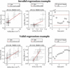 |
Fig. 1. Example of an invalid (top panels) and valid (bottom panels) derivation of γ satisfying all the criteria set for this study. The left and middle panels show the cross plots of ln(Tp) versus ln(np) and ln(np) versus ln(Tp), respectively, with the Wind data shown as black circles (and the corresponding standard deviation with error bars) and the regressed values as the solid red lines. The right panels show Bernoulli’s integral estimate for the same window (black circles) along with the 2% limit (dashed red lines). |
Finally, it is worth mentioning that the estimation of γ by fitting in lnT versus lnn is much more straightforward since it is based directly on measured quantities (Newbury et al. 1997; Kartalev et al. 2006). In contrast, fitting in lnP versus lnn would result in artefacts (biased correlations due to the fact that P is constructed from the measured n, thus not independently measured), and furthermore, the error propagation would result in significantly higher uncertainty.
4. Results
4.1. Distribution of the polytropic index within sheaths versus magnetic obstacles
Figure 2 shows the enriched histograms of the normalised occurrence (with respect to the total number of data) of the total, perpendicular, and parallel γ within 308 ICME sheaths (top panels) and 401 MOs (bottom panels), respectively. The enriched histograms allow for both the binned values and their uncertainties to be taken into account. Specifically, for its γ (and after the filtering discussed in the previous section), we generated a normally distributed set of 1000 values with a mean and sigma values corresponding to the original value and its uncertainty. This effectively changed the distribution of the original values, as their uncertainties were not considered previously (see also Livadiotis 2016, and discussion therein).
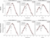 |
Fig. 2. Enriched histograms of the normalised occurrence (black circles) and κ-Gaussian distributions (red solid lines) of the (left to right) total, perpendicular, and parallel γ. The top and bottom panels correspond to ICME sheaths and MOs, respectively. At the top of each panel, the Pearson R and the RMSE of the fitted κ-Gaussian versus the normalised histogram values are also shown. |
We further note that there is a sharp dip in the histogram of the filtered values for γ ≈ 1, which corresponds to isothermal plasma. This is due to the filtering of the Pearson coefficient and the inverse polytropic index. For these intervals, when one parameter varies significantly while the other is nearly constant, the regression process fails because it cannot determine a slope close to zero (for the forward regression) or close to infinity (for the inverse regression). Further, this means that even though the derived γs were derived using the best fits, the filtering has also excluded real near-isothermal values (see also Nicolaou et al. 2014a, and discussion therein).
Therefore, in order to determine the average γ value of the distribution, we performed a weighted fitting focusing on its tails rather than its most frequent value. Following Livadiotis & McComas (2011) and Nicolaou et al. (2014a), we fit a κ-Gaussian distribution given by
![Mathematical equation: $$ \begin{aligned} f(\gamma ,\overline{\gamma },\kappa _{0},\sigma ) \propto \left[ 1 + \frac{\left( \gamma - \overline{\gamma }\right)^{2}}{\kappa _{0}\cdot \sigma ^{2}} \right]^{-\kappa _{0}-3/2}, \end{aligned} $$](/articles/aa/full_html/2025/03/aa52984-24/aa52984-24-eq3.gif) (3)
(3)
where  is the average polytropic index.
The weighted κ-Gaussian fit in the case of the ICME sheaths (top-left panel in Fig. 2) resulted in a slightly sub-adiabatic  . Furthermore, it is worth mentioning that the anisotropies (not shown here) were distributed with a mode near α ≈ 0.89 and a mean near α ≈ 0.87 (indicating a near-symmetric distribution), while plasma β values were distributed with a mode near β ≈ 0.56 and a mean near β ≈ 0.45. The latter values are in agreement with those found in the analysis of the entire Wind dataset by Katsavrias et al. (2024b), indicating that ICME sheaths exhibit (statistically) similar temperature anisotropy and plasma β conditions with the entire Wind dataset. The partial filtered polytropic index in the perpendicular direction (top-middle panel in Fig. 2) exhibits a very similar mean with the total polytropic index (
 ) but with a slightly increased σ, while the γ∥ distribution exhibits an increased mean (
 ) with a simultaneously broadening of the κ-Gaussian distribution (σ ≈ 2.65). The latter behaviour of the partial polytropic indices is also similar to the one revealed by Katsavrias et al. (2024b) for the entire Wind dataset, where the increased γ∥ was attributed to the decreased effective degrees of freedom in the parallel direction.
The weighted κ-Gaussian fit in the case of the ICME MOs (bottom-left panel in Fig. 2) resulted in a slightly increased  . The anisotropies (again not shown here) were distributed with a mode near α ≈ 0.89 and a mean near α ≈ 0.86 (very similar to the sheaths), while plasma β values were significantly decreased with a mode near β ≈ 0.11 and a mean near β ≈ 0.07. In contrast to the sheath region, MOs exhibit very similar partial polytropic indices with
  and
and  . The latter indicates that there is no significant deviation of the effective degrees of freedom in each direction. Nevertheless, our sample includes MOs that have structural differences with respect to the physics governing the plasma (e.g. LRFRs or ejecta with no clear rotation). Therefore, the aforementioned results describe plasmoids with different magnetic field properties mixed together.
4.2. Distribution of the polytropic index within sheaths with or without shock signature
Of the 308 sheaths included in our list of events, 155 are accompanied by a shock, while the rest (153 ICMEs) do not exhibit shock signatures. Figure 3 shows the normalised histograms and the weighted κ-Gaussian fit in the case of the ICME sheaths without a shock and the ICME sheaths that are accompanied by a shock (top and bottom panels, respectively). As shown, sheaths without a shock exhibit a  (similar to the γ exhibited by the full sheath sample), while the partial polytropic index in the perpendicular direction (top-middle panel in Fig. 3) exhibits a very similar mean. On the other hand, the γ∥ distribution exhibits a slightly increased mean (
 ) accompanied by a broadening of the κ-Gaussian distribution (right-top panel in Fig. 3).
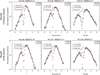 |
Fig. 3. Same as Fig. 2 but for ICME sheaths without and with shock, top and bottom panels respectively. |
The ICME sheaths, which are accompanied by shock (bottom panels in Fig. 3), exhibit a more sub-adiabatic  . Moreover, the partial polytropic index in the perpendicular and parallel direction (middle and right panel in Fig. 3) exhibit a
  and
and  . We note that even though the temperature anisotropy does not differ significantly with respect to the existence of a shock (αmode ≈ 0.89), there is a significant increase in plasma β values (not shown). In detail, the distribution of plasma β in sheaths without a shock exhibit a mean near β ≈ 0.38, while the respective distribution of plasma β in sheaths with a shock exhibit a significantly increased mean near β ≈ 0.52. This is expected, since shocks can result in much more turbulent plasma within the sheath, which in turn leads to the further decrease of the polytropic index from the adiabatic value. We also note again that the variation of the partial γ is in agreement with the results of Katsavrias et al. (2024b), that is, the perpendicular and parallel polytropic index exhibits decreased and increased values, respectively, due to the increase and decrease of the effective degrees of freedom in the corresponding direction for these β values.
In order to further investigate the effect of turbulence inside sheaths with shock, we divided the 155 sheaths into two parts of equal duration, and we repeated the methodology for the derivation of the  . As shown in Fig. 4, the near-shock sheath part exhibits a
  , while the near-MO sheath part exhibits a
  . The latter result indicates that turbulent heating is greater at larger distances from the shock region and near the MOs.
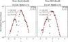 |
Fig. 4. Enriched histograms of the normalised occurrence (black circles) and κ-Gaussian distributions (red solid lines) of the total γ within the near-shock (left panel) and near-MO (right panel) sheath. On top of each panel, the Pearson R and the RMSE of the fitted κ-Gaussian versus the normalised histogram values are also shown. |
4.3. Distribution of the polytropic index within different magnetic obstacles
In order to reach more robust results on the thermodynamic behaviour of the MOs, we applied the same methodology to the various categories separately. Figure 5 shows the histograms and the weighted κ-Gaussian fits in the case of MOs with single flux ropes of various rotations. The SRFRs (top row of panels) exhibit a near adiabatic  . The partial polytropic indices exhibit a very small variation from the adiabatic value given the error of the estimated
  . As we moved to the flux ropes with a larger rotation, we observed an evident decrease of the polytropic index. For MRFRs (i.e. rotation between 90° and 180°), we derived a
  (middle row panels), while the LRFRs exhibit a
  (bottom row panels). The partial polytropic indices also exhibit a small variation from the total polytropic index value, while the partial polytropic index at the parallel direction always exhibits a broadening of the distribution (higher σ). A pronounced exception is the
  for the LRFRs, which deviates significantly towards more isothermal values at
  (bottom row right panel). Such behaviour could possibly imply an increase of the effective degrees of freedom in the parallel (with respect to the magnetic field) direction if we also consider the decrease of the anisotropy as we move from SRFRs to LRFRs (i.e. α ≈ 0.93, 0.86, and 0.84 for small, medium, and large rotation, respectively).
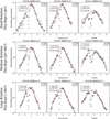 |
Fig. 5. Same as Fig. 2 but for different rotation flux ropes. Top to bottom: Rotation < 90°, rotation between 90°, and 180° and rotation > 180°, respectively. |
Figure 6 shows the histograms and the weighted κ-Gaussian fits in the case of non-flux-rope MOs. On top of each panel, we quantified the goodness of fit using the Pearson correlation coefficient between the histogram and the fit values as well as the root mean square error (RMSE), calculated as  ). As shown, complex MOs exhibit a
  (top row panels). The partial
  at the perpendicular direction exhibits a small increase (
 ), consistent with the behaviour of flux ropes. On the other hand, the partial
  at the parallel direction exhibits a significant increase reaching 1.89, with a simultaneous broadening of the distribution by more than a factor of two (σ ≈ 5.4). In contrast with flux ropes and complex MOs, the ejecta exhibit a completely different polytropic behaviour. As shown in the bottom panels of Fig. 6, the total polytropic index is slightly super-adiabatic (
 ). This
  is very similar to the results of Katsavrias et al. (2024b) and Livadiotis (2018), who estimated a
  and ≈1.86, respectively, for the solar wind. The partial
  at the perpendicular direction seems to exhibit a small decrease towards a more adiabatic value (≈1.66), while the partial
  at the parallel direction exhibits an increase with
  .
.
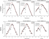 |
Fig. 6. Same as Fig. 2 but for non-flux-rope MOs. Top and bottom panels correspond to complex MOs and ejecta, respectively. |
5. Discussion
Using a list of 401 ICMEs identified from Wind measurements during more than two solar cycles (1995–2001), we performed a thorough investigation of the total and partial proton polytropic behaviour within the different ICME regions (i.e. sheaths and MOs). We further exploited the classification of the MOs with respect to the various magnetic field configurations inside the MOs to reveal any deviations among them. Our results are summarised in Table 1 and Fig. 7.
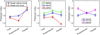 |
Fig. 7. Comparison of the total and partial polytropic index for the various sheaths and MOs. Left panel: sheaths without and with shock (blue and red stars, respectively). Middle panel: small, medium, and large rotation flux ropes with green, blue, and red circles, respectively. Right panel: medium rotation flux ropes (blue circles) and ejecta (magenta squares). |
Polytropic index, anisotropy (α) and plasma β values for the various ICME classifications.
The ICME sheath region contains more turbulent plasma compared to both the MO and the average solar wind (Kilpua et al. 2019). This is also depicted in the polytropic index, which exhibits sub-adiabatic values. Our analysis further reveals that sheaths accompanied by shocks exhibited a slightly more sub-adiabatic  compared to sheaths without a shock (
 ). This is attributed to the fact that shocks can, on average, result in much more turbulent plasma within the sheath, which is also supported by the increase of the average plasma β from 0.38 to 0.51 in sheaths without and with a shock, respectively. This result is further in agreement with Nicolaou et al. (2020) and Katsavrias et al. (2024b), who showed that there is an anti-correlation of the polytropic index with respect to plasma β. The aforementioned difference implies that the presence of the shock provides some coherence to the structures and may signify that they have gone through less evolution or interaction compared to the non-shocked sheaths (that are, presumably, evolving towards the ambient solar wind). Furthermore, it is worth mentioning that the distance from the shock also plays an important role, as the near-MO sheath part exhibits a significantly lower
  (≈1.46) compared to the near-shock part. Indeed, the trends in sub-adiabatic γ indicate that reconnection plays a role around the MOs by increasing heating and turbulence with distance. This is consistent with turbulence being modelled as an energy cascade process, where energy is injected at large scales, cascaded through inertial scales, and dissipated at small kinetic scales (Matthaeus et al. 1999; Andrés et al. 2019; Shaikh 2024). Even though further investigation on this matter is beyond the scope of this paper, this process may affect the drag (Subramanian et al. 2012; Bhattacharjee et al. 2022) that the MO is experiencing and, in principle, contribute to more efficient heating of particles (for energetic CMEs).
Moreover, our results are in qualitative agreement with Dayeh & Livadiotis (2022), who estimated a γ ≈ 1.4 for ICME sheaths. The relatively small disagreement between their results and those of this study could arise from the variation of plasma β. In detail, Dayeh & Livadiotis (2022) considered only a fraction of the ICME sheaths included in the Nieves-Chinchilla et al. (2019) list (i.e. only 25 events, and of these, 13 were accompanied by shock. The average plasma β was 0.52 for all 25 sheaths and 0.62 for the 13 sheaths accompanied by a shock, both of which are considerably higher values compared to our sample. Another source of this disagreement could be that in Dayeh & Livadiotis (2022) only parts of the sheaths that exhibited a small variation in the polytropic index were used, and it is possible that these parts originated at the near-MO sheath regions. Finally, the variation of the partial γ in sheaths is in agreement with the results of Katsavrias et al. (2024b). The latter authors indicated that the perpendicular and parallel polytropic index exhibits decreased and increased values, respectively due to the increase and decrease of the effective degrees of freedom in the corresponding direction. In our study, the existence of a shock seems to amplify the aforementioned effect (left panel of Fig. 7).
The MOs, on the other hand, on average exhibit a larger polytropic index compared to the sheaths indicating less turbulent heating. The polytropic behaviour of the protons inside the MOs is further dependent on the magnetic field configuration. The MOs that exhibit clear magnetic field rotation (flux ropes) exhibit generally sub-adiabatic proton  , which is further dependent on the magnitude of the rotation itself (i.e. the larger the rotation, the smaller the polytropic index). In particular, the LRFR category that exhibits rotations > 180° may represent events with significant curvature or distortion (Nieves-Chinchilla et al. 2018), which could explain the decreased
  due to increased turbulence. These results are again in qualitative agreement with the ones presented in Dayeh & Livadiotis (2022) since 18 out of the 25 events studied by the authors were MRFRs and LRFRs, and five of them were complex events. Furthermore, any quantitative disagreement falls within the error in our estimation of the
  . We note that the behaviour of the partial polytropic index (middle panel Fig. 7) follows the dependence on temperature anisotropy (Katsavrias et al. 2024b), with decreasing average anisotropy leading to higher effective degrees of freedom at the parallel direction and consequently a lower partial
  .
.
Following Katsavrias et al. (2024a), we connected the derived polytropic indices with the entropy gradient and the turbulent heating gradient (Livadiotis et al. 2020) at 1 AU. The proton entropy can be expressed in terms of proton density and temperature (Livadiotis 2019; Livadiotis & Nicolaou 2021) as
 (4)
(4)
where S is the entropy, deff are the effective degrees of freedom, n is the number density, and kB is the Boltzmann-Gibbs entropic measure (Livadiotis & McComas 2023). Furthermore, the density drop can be approximated as
 (5)
(5)
while the polytropic relation for isotropic temperature is
 (6)
(6)
Combining Eqs. (4), (5), and (6), we obtained
 (7)
(7)
where γα = 1 + 2/deff so that deff = 3 and γα = 5/3. Combining these equations, we express the entropy gradient as
 (8)
(8)
On the other hand, the gradient of the turbulent heating Et of the proton plasma (per mass), normalised by the thermal energy, is also equal to the deviation of the polytropic index from its adiabatic value (Verma et al. 1995; Livadiotis 2019),
 (9)
(9)
Here, Et is the turbulent heating of the proton plasma per mass, normalised by the thermal energy; S is the entropy; R is the radial distance; and kB is the Boltzmann-Gibbs entropic measure (Livadiotis & McComas 2023). The adiabatic polytropic index can be written as a function of the effective kinetic degrees of freedom as γα = 1 + 2/deff. More details on the connection of the polytropic index with the entropy gradient can be found in the appendix. Assuming that deff = 3 and γα = 5/3, even though deff may be affected by the temperature anisotropy (see also Livadiotis & Nicolaou 2021), the entropic gradient jump is three times the polytropic jump. The top panel Fig. 8 shows the polytropic and entropy jump in the case of MRFRs, which correspond to the most frequent MO structure in our list, preceded by sheaths accompanied by a shock. We note that we assumed an adiabatic solar wind with  . This is of course purely theoretical and valid for slow solar wind streams with isotropic temperature and three effective degrees of freedom. As shown, the entropic gradient jump (Δ(dS/dR)) from the theoretical adiabatic solar wind to the sheaths with shock is ≈0.39, while the entropic gradient jump from the sheaths to the MRFRs and then to the adiabatic solar wind is ≈−0.18 and −0.21, respectively.

On the other hand, ejecta (i.e. MOs with no clear magnetic field rotation) exhibit a super-adiabatic  , which is similar to the value found for the solar wind (Nicolaou et al. 2014a; Livadiotis 2018; Katsavrias et al. 2024b). Furthermore, the ejecta exhibit decreased and increased
  at the perpendicular and parallel direction, respectively (right panel Fig. 7), again similar to the sheaths and solar wind in general. We note that despite the fact that flux ropes are always expected based on the CME eruption theories (Vourlidas 2014), this is not always the case since changes during the interplanetary evolution might affect the magnetic field configuration inside the MO (Manchester et al. 2017; Nieves-Chinchilla et al. 2019). The increasing trend in
  from LRFR to MRFR to SRFR to ejecta indicates a progressive reduction in the coherence of the structures and/or an increasing flank crossing through the structure. The ejecta are clearly not flux ropes, but they are also not ambient solar wind (since plasma β is very low). Thus, the ejecta can be (1) destroyed flux ropes at the ejection (e.g. via a process similar to Chintzoglou et al. (2017)), (2) ambient structures carried away by the CME (DeForest et al. 2013), or (3) substantial reconnection during IP propagation (Pal et al. 2020; Stamkos et al. 2023). The bottom panel of Fig. 8 shows the polytropic and entropy jump in the case of ejecta preceded by sheaths accompanied by shock. As shown, the entropic gradient jump from the sheaths to the ejecta and then to the adiabatic solar wind is ≈ − 0.75 and 0.36, respectively.
Finally, we must note that CME regions, especially the ones associated with multiple acceleration mechanisms, may include various components such as suprathermal tails and beams that are not considered here due to the limitation of the dataset we used. To that end, we have included examples of velocity distributions for each of the ICME categories in this study (i.e. ejecta, SRFR, MRFR, and LRFR) inferred from the 3DP PESA low instrument (Lin et al. 1995; Wilson et al. 2021) on board Wind (see Figs. A.1–A.4). We emphasise that the different time periods satisfy all the criteria set in this study and are therefore accompanied by a valid polytropic index. As shown, these characteristic proton velocity distributions do not exhibit beams in the parallel direction. On the other hand, kappa tails are present in several instances (see, for example, the bottom panels in Fig. A.4). Nevertheless, even though kappa tails can contribute to ion density and temperature estimation, they cannot affect the derivation of the polytropic index. This is because the misestimation of the moments is constant for constant kappa (Nicolaou & Livadiotis 2016, 2019). This constant offset cannot affect the slope of the lnTp versus lnnp. In addition, we ensured (by requiring the stability of the Bernoulli integral) that each examined time window belongs to a single streamline characterised by a single polytropic index and kappa value (Livadiotis et al. 2018). Data from state-of-the-art missions such as Solar Orbiter and/or the Parker Solar Probe will allow for a much more thorough investigation in a future study. This will be especially interesting in radial distances closer to the Sun, where various distributions may contribute more effectively in solar wind proton thermodynamics.
6. Conclusions
We have performed a detailed investigation of the proton polytropic behaviour inside ICMEs using a list of 401 events identified from Wind measurements during more than two solar cycles (1995–2001). Our main conclusions are summarised as follows:
-
Sheaths are sub-adiabatic, indicating turbulent plasma with high plasma β values.
-
The value of the
 in sheaths depends on the existence of a shock and, consequently, the plasma β. Sheaths accompanied by a shock exhibit an average plasma β≈0.38 and a
  , while sheaths without a shock exhibit an average plasma β ≈ 0.51 and a
  1.57, indicating more turbulent heating.
 -
The value of the
 in sheaths accompanied by a shock further depends on the distance from the shock, as the near-shock parts exhibit a
  and the near-MO parts show a
  .
. -
The polytropic behaviour of the protons inside the MOs is dependent on the magnetic field configuration, e.g. LRFRs or ejecta with no observed rotation.
-
Flux ropes with a rotation above 90 degrees exhibit a sub-adiabatic polytropic index (
 and 1.54 for medium and large rotation, respectively), while SRFRs exhibit a near-adiabatic
  1.65. This probably indicates that the increased turbulence (due to the large rotation) leads to energy absorption (heating).
 -
Ejecta (non-flux-rope events) exhibit a super-adiabatic polytropic index (
 ) similar to the one found for the solar wind, supporting the scenario that changes during the interplanetary evolution might affect the magnetic field configuration inside the MO.
 -
Flux ropes, regardless of their rotation, exhibit a decreased
 in the parallel direction compared to the perpendicular direction. In contrast, ejecta exhibit an increased
  in the parallel direction, which is similar to what is exhibited by sheaths and solar wind in general.
 -
Assuming the transition from the theoretically adiabatic solar wind (γ≈1.67) to a sheath accompanied by a shock then to an MRFR and then back to the theoretically adiabatic solar wind, the entropic gradient (dS/dR) is +0.39 [kB/au], −0.18 [kB/au], and −0.21 [kB/au], respectively. The respective entropic gradient for the transition from a sheath with a shock to an ejecta and then to the theoretically adiabatic solar wind is −0.75 [kB/au], and −0.36 [kB/au], respectively.
Our results demonstrate that the variation of the polytropic index around and inside MOs may be used to track either the coherence of the MO or the distance from the centre, and hence it could serve as a guide to improve 3D reconstructions of these events. Finally, the analysis carried out in this work could be extended to in situ measurements closer to the Sun (i.e. from Solar Orbiter and the Parker Solar Probe) and thus allow for deeper physical understanding of the role of internal and ambient interactions on the magnetic structure of a CME en route to Earth.
Acknowledgments
The authors thank the National Space Science Data Center of the Goddard Space Flight Center for the use permission of Wind data and the NASA CDAWeb team for making these data available at http://cdaweb.gsfc.nasa.gov/istp_public/. ICME events used in this study are publicly available at https://wind.nasa.gov/ICME_catalog/ICME_catalog_viewer.php.
References
- Aminalragia-Giamini, S., Jiggens, P., Anastasiadis, A., et al. 2020, JSWSC, 10, 1 [NASA ADS] [Google Scholar]
- Andrés, N., Sahraoui, F., Galtier, S., et al. 2019, Physical Review Letters, 123, 245101 [CrossRef] [Google Scholar]
- Bhattacharjee, D., Subramanian, P., Nieves-Chinchilla, T., & Vourlidas, A. 2022, Monthly Notices of the Royal Astronomical Society, 518, 1185 [NASA ADS] [CrossRef] [Google Scholar]
- Borovsky, J. E., & Denton, M. H. 2006, J. Geophys. Res., 111, A07S08 [Google Scholar]
- Chandrasekhar, S. 1957, An Introduction to the Study of Stellar Structure Astrophysical Monographs (Dover Publications) [Google Scholar]
- Chintzoglou, G., Vourlidas, A., Savcheva, A., et al. 2017, The Astrophysical Journal, 843, 93 [NASA ADS] [CrossRef] [Google Scholar]
- Daglis, I. A., Katsavrias, C., & Georgiou, M. 2019, Philos. Trans. R. Soc. A, 377, 20180097 [NASA ADS] [CrossRef] [Google Scholar]
- Dayeh, M. A., & Livadiotis, G. 2022, ApJ, 941, L26 [NASA ADS] [CrossRef] [Google Scholar]
- DeForest, C. E., Howard, T. A., & McComas, D. J. 2013, The Astrophysical Journal, 769, 43 [NASA ADS] [CrossRef] [Google Scholar]
- Dialynas, K., Roussos, E., Regoli, L., et al. 2018, J. Geophys. Res., 123, 8066 [NASA ADS] [CrossRef] [Google Scholar]
- Elliott, H. A., McComas, D. J., Zirnstein, E. J., et al. 2019, ApJ, 885, 156 [Google Scholar]
- Ghag, K., Pathare, P., Raghav, A., et al. 2024, ASR, 73, 1064 [Google Scholar]
- Kartalev, M., Dryer, M., Grigorov, K., & Stoimenova, E. 2006, J. Geophys. Res., 111, A10107 [NASA ADS] [Google Scholar]
- Katsavrias, C., Daglis, I. A., Li, W., et al. 2015a, Ann. Geophys., 33, 1173 [NASA ADS] [CrossRef] [Google Scholar]
- Katsavrias, C., Daglis, I. A., Turner, D. L., et al. 2015b, Geophys. Res. Lett., 42, 10,521 [NASA ADS] [CrossRef] [Google Scholar]
- Katsavrias, C., Hillaris, A., & Preka-Papadema, P. 2016, ASR, 57, 22342244 [Google Scholar]
- Katsavrias, C., Nicolaou, G., Di Matteo, S., et al. 2024a, A&A, 686, L10 [NASA ADS] [CrossRef] [EDP Sciences] [Google Scholar]
- Katsavrias, C., Nicolaou, G., & Livadiotis, G. 2024b, A&A, 691, L11 [NASA ADS] [CrossRef] [EDP Sciences] [Google Scholar]
- Kilpua, E. K. J., Hietala, H., Turner, D. L., et al. 2015, Geophys. Res. Lett., 42, 3076 [NASA ADS] [CrossRef] [Google Scholar]
- Kilpua, E. K. J., Fontaine, D., Moissard, C., et al. 2019, Space Weather, 17, 1257 [NASA ADS] [CrossRef] [Google Scholar]
- Kuhn, S., Kamran, M., Jelić, N., et al. 2010, AIP Conference Proceedings (AIP), 1306, 216 [NASA ADS] [CrossRef] [Google Scholar]
- Lepping, R. P., Acũna, M. H., Burlaga, L. F., et al. 1995, Space Sci. Rev., 71, 207 [Google Scholar]
- Lin, R. P., Anderson, K. A., Ashford, S., et al. 1995, Space Science Reviews, 71, 125 [NASA ADS] [CrossRef] [Google Scholar]
- Liu, Y., Richardson, J., & Belcher, J. 2005, PSS, 53, 3 [Google Scholar]
- Livadiotis, G. 2015, ApJ, 809, 111 [NASA ADS] [CrossRef] [Google Scholar]
- Livadiotis, G. 2016, ApJS, 223, 13 [NASA ADS] [CrossRef] [Google Scholar]
- Livadiotis, G. 2018, Entropy, 20, 799 [NASA ADS] [CrossRef] [Google Scholar]
- Livadiotis, G. 2019, Stats, 2, 416 [CrossRef] [Google Scholar]
- Livadiotis, G., & McComas, D. J. 2011, ApJ, 741, 88 [NASA ADS] [CrossRef] [Google Scholar]
- Livadiotis, G., & McComas, D. J. 2013, J. Geophys. Res., 118, 2863 [NASA ADS] [CrossRef] [Google Scholar]
- Livadiotis, G., & McComas, D. J. 2023, Sci. Rep., 13, 9033 [NASA ADS] [CrossRef] [Google Scholar]
- Livadiotis, G., & Nicolaou, G. 2021, ApJ, 909, 127 [NASA ADS] [CrossRef] [Google Scholar]
- Livadiotis, G., Desai, M. I., & Wilson, L. B. 2018, The Astrophysical Journal, 853, 142 [NASA ADS] [CrossRef] [Google Scholar]
- Livadiotis, G. P., Dayeh, M. A., & Zank, G. 2020, ApJ, 905, 137 [NASA ADS] [CrossRef] [Google Scholar]
- Manchester, W., Kilpua, E. K. J., Liu, Y. D., et al. 2017, Space Sci. Rev., 212, 1159 [Google Scholar]
- Matthaeus, W. H., Zank, G. P., Smith, C. W., & Oughton, S. 1999, Physical Review Letters, 82, 3444 [NASA ADS] [CrossRef] [Google Scholar]
- Mishra, W., & Wang, Y. 2018, ApJ, 865, 50 [NASA ADS] [CrossRef] [Google Scholar]
- Newbury, J. A., Russell, C. T., & Lindsay, G. M. 1997, GRL, 24, 1431 [NASA ADS] [CrossRef] [Google Scholar]
- Nicolaou, G., & Livadiotis, G. 2016, Astrophysics and Space Science, 361, 359 [NASA ADS] [CrossRef] [Google Scholar]
- Nicolaou, G., & Livadiotis, G. 2019, ApJ, 884, 52 [NASA ADS] [CrossRef] [Google Scholar]
- Nicolaou, G., Livadiotis, G., & Moussas, X. 2014a, Sol. Phys., 289, 1371 [NASA ADS] [CrossRef] [Google Scholar]
- Nicolaou, G., McComas, D. J., Bagenal, F., & Elliott, H. A. 2014b, J. Geophys. Res., 119, 3463 [NASA ADS] [CrossRef] [Google Scholar]
- Nicolaou, G., Livadiotis, G., & Wicks, R. T. 2019, Entropy, 21, 997 [NASA ADS] [CrossRef] [Google Scholar]
- Nicolaou, G., Livadiotis, G., Wicks, R. T., Verscharen, D., & Maruca, B. A. 2020, ApJ, 901, 26 [CrossRef] [Google Scholar]
- Nicolaou, G., Livadiotis, G., & McComas, D. J. 2023, The Astrophysical Journal, 948, 22 [NASA ADS] [CrossRef] [Google Scholar]
- Nieves-Chinchilla, T., Vourlidas, A., Raymond, J. C., et al. 2018, Sol. Phys., 293, 25 [NASA ADS] [CrossRef] [Google Scholar]
- Nieves-Chinchilla, T., Jian, L. K., Balmaceda, L., et al. 2019, Sol. Phys., 294, 89 [Google Scholar]
- Ogilvie, K. W., Chornay, D. J., Fritzenreiter, R. J., et al. 1995, Space Sci. Rev., 71, 55 [Google Scholar]
- Pal, S., Dash, S., & Nandy, D. 2020, Geophysical Research Letters, 47, e86372 [NASA ADS] [Google Scholar]
- Parker, E. N. 1961, ApJ, 134, 20 [NASA ADS] [CrossRef] [Google Scholar]
- Parker, E. 1963, Interplanetary Dynamical Processes, Interscience Monographs and Texts in Physics and Astronomy (Interscience Publishers) [Google Scholar]
- Scherer, K., Fichtner, H., Fahr, H. J., Röken, C., & Kleimann, J. 2016, ApJ, 833, 38 [NASA ADS] [CrossRef] [Google Scholar]
- Shaikh, Z. I. 2024, Monthly Notices of the Royal Astronomical Society, 530, 3005 [NASA ADS] [CrossRef] [Google Scholar]
- Siegel, A. F. 1982, Biometrika, 69, 242 [NASA ADS] [CrossRef] [Google Scholar]
- Stamkos, S., Patsourakos, S., Vourlidas, A., & Daglis, I. A. 2023, Solar Physics, 298, 88 [NASA ADS] [CrossRef] [Google Scholar]
- Subramanian, P., Lara, A., & Borgazzi, A. 2012, Geophysical Research Letters, 39, L19107 [NASA ADS] [CrossRef] [Google Scholar]
- Totten, T. L., Freeman, J. W., & Arya, S. 1995, Journal of Geophysical Research: Space Physics, 100, 13 [NASA ADS] [CrossRef] [Google Scholar]
- Turner, D. L., Shprits, Y., Hartinger, M., & Angelopoulos, V. 2012, Nature Physics, 8, 208 [NASA ADS] [CrossRef] [Google Scholar]
- Turner, D. L., Kilpua, E. K. J., Hietala, H., et al. 2019, J. Geophys. Res., 124, 1013 [NASA ADS] [CrossRef] [Google Scholar]
- Verma, M. K., Roberts, D. A., & Goldstein, M. L. 1995, J. Geophys. Res., 100, 19839 [NASA ADS] [CrossRef] [Google Scholar]
- Vourlidas, A. 2014, Plasma Phys. Control. Fusion, 56, 064001P [CrossRef] [Google Scholar]
- Wilson, L. B., Brosius, A. L., Gopalswamy, N., et al. 2021, Reviews of Geophysics, 59, e2020RG000714 [NASA ADS] [CrossRef] [Google Scholar]
- Zurbuchen, T. H., & Richardson, I. G. 2006, Space Sci. Rev., 123, 31 [Google Scholar]
Appendix A: Velocity distributions
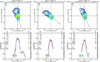 |
Fig. A.1. Examples of velocity distributions during the ejecta event on November 11, 2000 at three time intervals. (Top panels) 3D ion distribution of velocity analyzed to components parallel and perpendicular to the magnetic field, respectively. (Bottom panels) Parallel and perpendicular cuts of the 3D distribution in red and blue triangles, respectively. |
All Tables
Polytropic index, anisotropy (α) and plasma β values for the various ICME classifications.
All Figures
|
Fig. 1. Example of an invalid (top panels) and valid (bottom panels) derivation of γ satisfying all the criteria set for this study. The left and middle panels show the cross plots of ln(Tp) versus ln(np) and ln(np) versus ln(Tp), respectively, with the Wind data shown as black circles (and the corresponding standard deviation with error bars) and the regressed values as the solid red lines. The right panels show Bernoulli’s integral estimate for the same window (black circles) along with the 2% limit (dashed red lines). |
| In the text | |
|
Fig. 2. Enriched histograms of the normalised occurrence (black circles) and κ-Gaussian distributions (red solid lines) of the (left to right) total, perpendicular, and parallel γ. The top and bottom panels correspond to ICME sheaths and MOs, respectively. At the top of each panel, the Pearson R and the RMSE of the fitted κ-Gaussian versus the normalised histogram values are also shown. |
| In the text | |
|
Fig. 3. Same as Fig. 2 but for ICME sheaths without and with shock, top and bottom panels respectively. |
| In the text | |
|
Fig. 4. Enriched histograms of the normalised occurrence (black circles) and κ-Gaussian distributions (red solid lines) of the total γ within the near-shock (left panel) and near-MO (right panel) sheath. On top of each panel, the Pearson R and the RMSE of the fitted κ-Gaussian versus the normalised histogram values are also shown. |
| In the text | |
|
Fig. 5. Same as Fig. 2 but for different rotation flux ropes. Top to bottom: Rotation < 90°, rotation between 90°, and 180° and rotation > 180°, respectively. |
| In the text | |
|
Fig. 6. Same as Fig. 2 but for non-flux-rope MOs. Top and bottom panels correspond to complex MOs and ejecta, respectively. |
| In the text | |
|
Fig. 7. Comparison of the total and partial polytropic index for the various sheaths and MOs. Left panel: sheaths without and with shock (blue and red stars, respectively). Middle panel: small, medium, and large rotation flux ropes with green, blue, and red circles, respectively. Right panel: medium rotation flux ropes (blue circles) and ejecta (magenta squares). |
| In the text | |
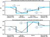 |
Fig. 8. Estimated entropic gradient jumps and |
| In the text | |
|
Fig. A.1. Examples of velocity distributions during the ejecta event on November 11, 2000 at three time intervals. (Top panels) 3D ion distribution of velocity analyzed to components parallel and perpendicular to the magnetic field, respectively. (Bottom panels) Parallel and perpendicular cuts of the 3D distribution in red and blue triangles, respectively. |
| In the text | |
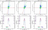 |
Fig. A.2. same as figure A.1 during the SRFR event on December 25, 2007. |
| In the text | |
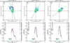 |
Fig. A.3. same as figure A.1 during the MRFR event on April 20, 2002. |
| In the text | |
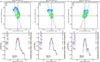 |
Fig. A.4. same as figure A.1 during the LRFR event on May 28, 2011. |
| In the text | |
Current usage metrics show cumulative count of Article Views (full-text article views including HTML views, PDF and ePub downloads, according to the available data) and Abstracts Views on Vision4Press platform.
Data correspond to usage on the plateform after 2015. The current usage metrics is available 48-96 hours after online publication and is updated daily on week days.
Initial download of the metrics may take a while.