| Issue |
A&A
Volume 698, May 2025
|
|
|---|---|---|
| Article Number | A79 | |
| Number of page(s) | 14 | |
| Section | The Sun and the Heliosphere | |
| DOI | https://doi.org/10.1051/0004-6361/202452866 | |
| Published online | 29 May 2025 | |
Evolution of the interacting coronal mass ejections that drove the great geomagnetic storm of 10 May 2024
1
Indian Institute of Astrophysics, II Block, Koramangala, Bengaluru 560034, India
2
Pondicherry University, R.V. Nagar, Kalapet, 605014 Puducherry, India
⋆ Corresponding author: soumyaranjan.khuntia@iiap.res.in
Received:
4
November
2024
Accepted:
29
March
2025
Context. The arrival of a series of coronal mass ejections (CMEs) at the Earth resulted in a great geomagnetic storm on 10 May 2024, the strongest storm in the last two decades.
Aims. We investigated the kinematic and thermal evolution of the successive CMEs to understand their interaction en route to Earth. We attempted to find the dynamic, thermodynamic, and magnetic field signatures of CME-CME interactions. Our focus was to compare the thermal state of CMEs near the Sun and in their post-interaction phase at 1 AU.
Methods. The 3D kinematics of six identified Earth-directed CMEs were determined using the graduated cylindrical shell (GCS) model. The flux rope internal state (FRIS) model was implemented to estimate the CMEs’ polytropic index and temperature evolution from their measured kinematics. The thermal states of the interacting CMEs were examined using in situ observations from the Wind spacecraft at 1 AU.
Result Our study determined the interaction heights of selected CMEs and confirmed their interactions that led to the formation of complex ejecta identified at 1 AU. The plasma, magnetic field, and thermal characteristics of magnetic ejecta (MEs) within the complex ejecta and other substructures, such as interaction regions within two MEs and double flux rope-like structures within a single ME, show possible signatures of CME-CME interaction in in situ observations. The FRIS-model-derived thermal states of individual CMEs reveal their diverse thermal evolution near the Sun, with all CMEs transitioning to an isothermal state at 6–9 R⊙ except for CME4, which was in an adiabatic state due to a lower expansion rate. The electrons of the complex ejecta at 1 AU are in a predominant heat-release state, while the ions show a bimodal distribution of thermal states. On comparing the characteristics of CMEs near the Sun and at 1 AU, we suggest that such a one-to-one comparison is difficult due to the CME-CME interactions significantly influencing the CMEs’ post-interaction characteristics.
Key words: Sun: corona / Sun: coronal mass ejections (CMEs) / Sun: heliosphere / solar-terrestrial relations / solar wind
© The Authors 2025
 Open Access article, published by EDP Sciences, under the terms of the Creative Commons Attribution License (https://creativecommons.org/licenses/by/4.0), which permits unrestricted use, distribution, and reproduction in any medium, provided the original work is properly cited.
This article is published in open access under the Subscribe to Open model. Subscribe to A&A to support open access publication.
1. Introduction
Coronal mass ejections (CMEs) are dynamic eruptions from the Sun that release enormous quantities of magnetized plasma into interplanetary space (Hundhausen et al. 1984; Webb & Howard 2012; Temmer et al. 2023; Mishra & Teriaca 2023). When CMEs travel farther from the Sun into interplanetary space, they are traditionally known as interplanetary coronal mass ejections (ICMEs). These solar events can cause prolonged geomagnetic storms, disrupting essential societal infrastructure such as communication systems, power grid systems, and satellite operations, and pose significant risks to our technology-dependent society (Gonzalez et al. 1994; Pulkkinen 2007). Therefore, two of the primary research objectives in the CME-related field are to forecast arrival times and evaluate the impact at Earth.
The initial speed of a CME, ranging from 100 to 3000 km s−1 (Yashiro et al. 2004) within 30 R⊙, can be decided based on the maximum energy that is available from an active region (Gopalswamy et al. 2005). However, by the time most CMEs reach Earth, their speeds have reduced to typically around 500–600 km s−1 (Richardson & Cane 2010). Furthermore, the kinematics, thermodynamics, radial expansion magnetic properties, and geo-effective parameters of a CME can also change during its evolution as it propagates away from the Sun (Liu et al. 2006; Kilpua et al. 2017; Mishra et al. 2020, 2021a; Khuntia et al. 2023; Agarwal & Mishra 2024). This suggests that while the active region near the Sun influences how powerful a CME can be, understanding its evolution through interplanetary space is crucial to determining its final impact on Earth. Furthermore, the interaction of a CME with another CME or a preconditioned ambient medium can significantly influence its plasma parameters, arrival time, and geo-effectiveness (Liu et al. 2014; Lugaz et al. 2017; Desai et al. 2020; Mishra et al. 2021b; Koehn et al. 2022; Temmer et al. 2023). Extensive case studies on interacting CMEs in interplanetary space have been conducted to better understand the changes in their morphology, arrival time, and consequences (Wang et al. 2003; Mishra & Srivastava 2014; Temmer et al. 2014; Mishra et al. 2015a, 2017; Scolini et al. 2020). However, the exact role of CME-CME interactions in governing the formation of merged ejecta, distinct structures, and their thermodynamic evolution in interplanetary space is still not fully understood.
Understanding the kinematic and thermodynamic parameters of CMEs near the Earth is important as the magnetic reconnection between the CME’s southward directed magnetic field and Earth’s northward pointing magnetic field facilitates the transfer of energy and plasma within Earth’s magnetosphere (Dungey 1961; Tsurutani et al. 1988). The intensity of geomagnetic storms is often represented by the disturbance storm time (Dst) index (Nose et al. 2015), which quantifies the perturbation in the horizontal component of the geomagnetic field at equatorial latitudes. A geomagnetic storm is classified as “great” if it reaches a minimum Dst index value of −350 nT or lower (Gonzalez et al. 2011; Mishra et al. 2024). Since the beginning of the space age, around 1957, there have only been 11 cases when the Dst index went below −350 nT (Meng et al. 2019). The most intense geomagnetic storm recorded by the Dst index is the March 1989 storm, which reached a minimum Dst index of −589 nT. This caused significant space weather hazards, including a blackout of the Canadian Hydro-Québec power system (Boteler 2019). A great storm occurred in November 2004, with a minimum Dst index value of −373 nT (Yermolaev et al. 2008). Two severe storms also took place in October 2003, registering minimum Dst index values of −363 nT and −401 nT, followed by another major storm in November 2003 with a minimum Dst index value of −472 nT (Gopalswamy et al. 2005; Srivastava et al. 2009). Such great geomagnetic storms are very rare, so statistically analyzing the properties of their drivers is a significant challenge. Therefore, it is important to analyze the individual great storms as they happen and examine their drivers if they exhibit significantly different properties.
Recent studies, based on both ground station and space satellite data, have reported various impacts of the 10 May 2024 great geomagnetic storm, such as an increase in the dayside ionospheric total electron content (TEC), low latitude aurorae, radio blackouts, and satellite drag (Gonzalez-Esparza et al. 2024; Hajra et al. 2024; Hayakawa et al. 2025; Lazzús & Salfate 2024; Spogli et al. 2024; Parker & Linares 2024; Jain et al. 2025). Weiler et al. (2025) studied the kinematics of the responsible CMEs and demonstrated that sub-L1 missions would have been able to effectively predict the strength of this geomagnetic storm up to 2.57 hours in advance, especially for strongly interacting events, which are still difficult to forecast. Liu et al. (2024) called it a “perfect storm” and highlighted the contrasting magnetic fields and geo-effectiveness of the complex structures at two different vantage points, even with only a mesoscale separation between them.
We analyzed the CMEs that potentially drove the great geomagnetic storm, the largest one in the last two decades, which started on 10 May 2024 and reached a minimum Dst index of −406 nT on 11 May 2024. In Sect. 2 we examine the near-Sun observations, estimating the 3D kinematics of successive CMEs associated with the great storm and focusing on their potential interactions en route to Earth. We also derive the near-Sun thermodynamic evolution of these interacting CMEs by combining remote observations with models. In Sect. 3 we analyze the in situ storm observations near Earth and disentangle the associated structures. We also study the thermal state evolution across the complex structure and ambient solar wind. Finally, in Sect. 4 we summarize the results, highlighting the key findings from both remote and in situ observations.
2. Near-Sun observations
In May 2024, the Sun experienced significant activity due to the emergence of a complex (βγδ) active region formed from the merging of NOAA active regions 13664 and 13668. Even after completing a full solar rotation, this active region produced numerous energetic flares. Based on in situ measured flow speed of ≈700–1000 km s−1 at 1 AU around the onset of the geomagnetic storm on 10 May 2024, we investigated potential halo and partial halo CME ejections from the Sun on 8–9 May 2024. We used coronagraph data from the COR2 telescope on the Sun-Earth Connection Coronal and Heliospheric Investigation (SECCHI; Howard et al. 2008) on board the Solar Terrestrial Relations Observatory Ahead (STEREO-A; Kaiser et al. 2008) and the Large Angle Spectroscopic Coronagraph (LASCO; Brueckner et al. 1995) on board the Solar and Heliospheric Observatory (SOHO; Domingo et al. 1995) to identify probable Earth-directed CMEs that might have erupted from the Sun 2–3 days before the start of geomagnetic storm. During our investigation period, STEREO-A was located ≈12° west of the Sun-Earth line, and it provided a similar view of the CMEs as from the SOHO viewpoint. Furthermore, we searched for corresponding activity on the solar disk using extreme ultra-violet imagery from the Atmospheric Imaging Assembly (AIA; Lemen et al. 2012) instrument on board the Solar Dynamics Observatory (SDO; Pesnell et al. 2012) to locate the associated source region. By analyzing the source locations and speed profiles, we identified six potential CMEs that could have contributed to the great event, as shown in Table 1. The selected CMEs were ejected on 8-9 May 2024 (The first appearance of CMEs on LASCO/C2 is shown in the second column of Table 1). Furthermore, we associated these CMEs with their corresponding flares and filaments by assessing the timing of the brightest flare or filament and evaluating the likelihood of them being the source. Out of the six CMEs, only CME3 is associated with a filament eruption in active region 13667, located at N25E14; the remaining CMEs are flare-related and originate from active region 13664 (third and fourth column in Table 1).
CMEs responsible for the great geomagnetic storm on 10 May 2024.
2.1. Determining 3D kinematics using white-light observations
We applied the graduated cylindrical shell (GCS) model (Thernisien et al. 2006; Thernisien 2011) to determine the 3D leading edge (LE) height (h) and direction of the CMEs. The GCS model provides a simplified geometric framework that represents a CME’s magnetic flux rope (FR) topology in space. This model has routinely been used to mitigate the observed projection effect in CME kinematics (Liu et al. 2010; Wang et al. 2014; Mishra et al. 2015a). This model takes advantage of fitting the CME envelope with simultaneous observations from multiple vantage points to obtain a better understanding of the CME kinematics. Our work used the contemporaneous coronagraphic observations from STEREO-A/COR2 and SOHO/LASCO-C2 & C3. The GCS-fitted coronagraphic images are shown in Fig. 1.
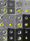 |
Fig. 1. GCS-model-fitted Earth-impacting CMEs responsible for the great event on 10 May 2024. Top panels: Running-difference imaging observations of CMEs from SOHO/LASCO-C2 and STEREO-A/SECCHI-COR2. Bottom panels: Fitted GCS model overlaid as the yellow wire frame. |
The LE heights and geometrical and positional parameters obtained from the GCS model fitting of the selected CMEs are given in Table 1. CME3, with the GCS model-derived source location of N04E24, erupted from the northeast side of the solar disk, while all other CMEs erupted from the southwest side. We find no substantial change in the tilt angle, aspect ratio, or half angle within our observed field of view. The errors mentioned in Table 1 for the GCS-fitted parameters were calculated by repeating the fitting process multiple times. Moreover, it is challenging to quantify the error associated with the GCS model, as the fitting process is performed manually and depends on the user’s experience and interpretation of the event. Thernisien et al. (2009) estimated the mean errors in the GCS model to be approximately ±4.3°, ±1.8°, ±22°, −7°+13°, −0.04°+0.07°, ±0.48 R⊙ for longitude, latitude, tilt angle, half angle (α), aspect ratio (k), and LE height, respectively.
The LE speed (v) and acceleration (a) of the selected CMEs (Fig. 2) are calculated by doing successive time derivatives of the measured 3D LE height (h). We applied a moving three-point window, and a linear fit was used within each window to compute the time derivatives at the middle point of the window. For the endpoints (first and last points), derivatives were determined similarly using a two-point window. This method, as described in detail in Agarwal & Mishra (2024), allows us to accurately capture reasonable fluctuations in speed and acceleration without decreasing the number of data points in the derivatives. The last column in Table 1 shows the maximum speed derived for each CME using the GCS model in the observed field of view. Furthermore, to quantify the error in the LE height, we considered the CME’s sharp LE near the Sun and its more diffuse edge at greater heights. Through multiple fitting attempts, we estimated a maximum uncertainty of ±10% for the LE height, and this error was propagated to derive the kinematic parameters, such as speed and acceleration. Figure 2a shows interesting findings that the last CME, CME6, has a higher speed compared to the others, suggesting a potential interaction at greater heights.
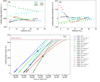 |
Fig. 2. Propagation speed (a) and acceleration (b) of LE of the selected CMEs derived from the GCS-model-fitted 3D LE heights. (c) Height-time profiles of the CMEs assuming no acceleration (solid line) and some value of a constant average deceleration (dashed line). The color-filled circles indicate the first possible CME-CME interaction height. The initial dots show the GCS-fitted heights for the CMEs. We include only every other data point for the GCS-fitted heights for the sake of clarity. |
Furthermore, we extrapolated the GCS-model-derived 3D LE height for each CME using a constant acceleration up to a height of 218 R⊙. The extrapolation of CME height was carried out using the following two approaches: (i) We chose the acceleration to be 0, meaning the CMEs propagate with a constant speed beyond the last tracked height of LE from the GCS model. (ii) We used the equation of motion with constant acceleration: s = ut + at2/2, where u is the speed of CME LE at the last tracked height from the GCS model, s is the height difference between the last tracked height and 218 R⊙, and t is the time interval between the arrival of CME LE at the last GCS-model-tracked height and at near-earth in situ spacecraft. The arrival of individual CMEs LE at in situ spacecraft is identified based on several plasma and magnetic field parameters, which is discussed in Sect. 3. The extrapolation, in the case of nonzero acceleration, is to match the estimates of CME arrival time with the observed CME/magnetic ejecta (ME)LE arrival time at 1 AU. In cases of non-zero acceleration, the extrapolation is performed to match the estimated CME arrival time with the observed arrival time of the CME leading edge at 1 AU. The approach of extrapolation with zero acceleration would only be valid before the CMEs interacted and cannot provide correct estimates of their arrival at 1 AU. However, extrapolation with zero acceleration, together with derived nonzero acceleration, can help determine the possible height range for CME-CME interactions. In general, fast CMEs reach their peak speed within a height of 10 R⊙ and show most of their acceleration up to 20 R⊙ (Zhang et al. 2004; Vršnak & Žic 2007; Temmer et al. 2010). This result can also be seen in Fig. 2b; the LE acceleration for all the CMEs decreases and tends toward a lower value. The CMEs primarily experienced aerodynamic drag at larger heights due to interaction with the solar wind. This drag force tends to accelerate the slow CMEs and decelerate the fast CMEs (Gopalswamy et al. 2000; Vršnak & Žic 2007). Thus, we can expect that zero acceleration will serve as an upper bound for kinematics.
Without involving any complex approach for estimating the dynamics of the selected CMEs in a varying ambient solar wind, we derived the kinematics for the CMEs beyond coronagraphic heights by extrapolating the measured kinematics from the GCS model to get the range of possible heights for CME-CME interaction. Obviously, the kinematics of the CMEs after their possible interaction cannot be represented by the extrapolated kinematic profiles of each CME. It is also possible that different CMEs experience different preconditioned media and follow varying acceleration profiles during their journey in both the pre-and post-interaction phases (Shen et al. 2012; Mishra et al. 2017). However, a simple extrapolation of kinematics can serve the scenario of possible interactions and can help interpret the in situ observations of structures at 1 AU driving the great geomagnetic storm. Figure 2c shows the estimated kinematics for each CME up to 218 R⊙. We note that there is not much difference in the GCS model derived LE speed for both CME1 and CME2 at 22 R⊙ (Fig. 2a). However, as CME1 is propagating ahead of CME2, CME1 is likely to get a higher drag and deceleration at higher heights than CME2. Moreover, the source longitude of CME1 and CME2 are 16 ± 3 and 13 ± 2, respectively. Hence, there is a possibility that the LE of CME2 will catch up with the back of CME1. Considering the derived acceleration of a = –1.78 m s−2 and a = –0.71 m s−2 for CME1 and CME2, respectively, they are predicted to interact at height ≈144 R⊙. There is an early interaction between CME3 and CME4 at a LE height of ≈54 R⊙ (considering a = 0 m s−2). Considering the longitude of the source region for CME3 and CME4, they are more likely to have a flank interaction. This interaction can also be seen in the LASCO C3 coronagraphic view. Furthermore, the derived kinematics also show the interaction between CME5 and CME6 at ≈110 R⊙. The interaction is possible primarily considering the faster speed of CME6 than CME5 and their close longitude source regions. If CME6 continues to maintain its high speed even after the interaction (as indicated by the faster speed of the trailing MEs observed at 1 AU), it suggests that all contributing CMEs likely interacted with one another en route to Earth. This interaction would have resulted in a large-scale complex magnetic structure to be observed at 1 AU, which is further discussed in the upcoming sections.
We note that our approach assumes a constant acceleration throughout the CME evolution beyond the coronagraphic heights to get a broad range of distances for possible CME-CME interaction. The estimated heights for different interacting CME pairs can change if we consider the drag force between an individual CME and ambient medium, momentum exchange during interacting CME pairs, and possibly magnetic interaction between closely separated CMEs. A detailed study using Heliospheric Imager (HI) observations and focusing more on the momentum exchange and nature of interaction/collision for interacting CMEs (Mishra et al. 2015a, 2017), geo-effectiveness (Lugaz & Farrugia 2014; Scolini et al. 2020) can reveal more insight into the complex ejecta evolution. The changes in the kinematics of CMEs will have imprints on their thermal state, which we discuss in the next section.
2.2. Determining thermodynamics using the measured 3D kinematics
Thermodynamics of successively launched CMEs from the same active region is not well understood, and further, there are limited studies to estimate the thermodynamic properties of different substructures of complex ejecta formed due to possible CME-CME interaction before they reach 1 AU. We applied an analytical model, the flux rope internal state (FRIS) model (Mishra & Wang 2018; Khuntia et al. 2023, 2024), to derive the internal thermal properties of the selected CMEs. The model considers the CME to have an axisymmetric cylindrical shape at a local scale and evolve as a polytropic process. The model conserves mass and angular momentum while assuming a self-similar evolution. The model solves the ideal magnetohydrodynamic equations of motion for the FR, incorporating various internal forces responsible for expanding the CME, such as the Lorentz force, thermal pressure force, and centrifugal force. As the model assumes the FR plasma is a single species magnetic fluid, the model-derived parameters show the average properties of the CME as a whole, both for protons and electrons. The model uses the global kinematics, such as height and radius of the CME FR, to derive various internal parameters, summarized in Table 1 of Khuntia et al. (2023).
We implemented the measured 3D kinematics in the FRIS model using the procedure mentioned in Khuntia et al. (2023). The equation of motion for the radial expansion of the CME FR can be expressed as
![$$ \begin{aligned} \frac{R}{L} =&{ c_5 \biggl [\frac{a_e R^2}{L}\biggr ]} - {c_3 c_5 \biggl [\frac{R}{L^2}\biggr ]} - {c_2 c_5\biggl [\frac{1}{R}\biggr ]} - {c_1 c_5\biggl [\frac{1}{LR}\biggr ]}{\nonumber }\\&+ c_4 \biggl [\frac{\mathrm{d}a_e}{\mathrm{d}t} + {\frac{(\gamma -1)a_e { v}_c}{L}} + \frac{(2\gamma -1)a_e { v}_e}{R}\biggr ] {\nonumber }\\&+ c_3 c_4\biggl [ \frac{(2-\gamma ) { v}_c }{L^2 R} + {\frac{(2-2\gamma ) { v}_e }{LR^2}}\biggr ] {\nonumber }\\&+ c_2 c_4\biggl [{\frac{(4-2\gamma ) { v}_e L}{R^4}} - {\frac{\gamma { v}_c}{R^3}}\biggr ] {\nonumber }\\&+ c_1 c_4\biggl [{\frac{(4-2\gamma ) { v}_e}{R^4}} + {\frac{(1-\gamma ){ v}_c}{LR^3}}\biggr ], \end{aligned} $$](/articles/aa/full_html/2025/06/aa52866-24/aa52866-24-eq1.gif)
where the inputs to the FRIS model are the distance of the center of the FR from the surface of the Sun (L), the radius of the FR (R), and their successive time derivatives, such as propagation speed (vc) and acceleration (ac) of the axis of the FR, expansion speed (ve) and acceleration (ae) of the FR. γ is the adiabatic index (γ = 5/3 for monatomic ideal gases), and c1 − c5 are unknown constants coefficients, whose values can be obtained by fitting Eq. (1). The fitting results for all the six selected CMEs are shown in Fig. A.1. Among the several internal properties that can be derived using the FRIS model, for this study, we focused on the evolution of two critical properties, such as the polytropic index (Γ) and temperature (T) of the selected CMEs. The model-derived expression for Γ and T are
![$$ \begin{aligned} \Gamma = \gamma + \frac{ln{\frac{\lambda (t)}{\lambda (t+\Delta t)}}}{ln[(\frac{L(t+\Delta t)}{L(t)})[\frac{R(t+\Delta t)}{R(t)}]^2]} \end{aligned} $$](/articles/aa/full_html/2025/06/aa52866-24/aa52866-24-eq2.gif)
![$$ \begin{aligned} {T}= \frac{ k_2 k_8 }{k_4 } \biggl [ \frac{\pi \sigma }{(\gamma -1)} {\lambda (LR^2)^{1{-\gamma }} }\biggr ]. \end{aligned} $$](/articles/aa/full_html/2025/06/aa52866-24/aa52866-24-eq3.gif)
Excluding L, R, and γ, all other quantities in the above equations are unknown (for details, see Khuntia et al. 2023). By determining the fitting coefficients for Eq. (1), some of those quantities can be evaluated. Thus, apart from γ, the temperature (T) estimates from the model are multiplied by a factor ( ), the absolute value of which could not be derived from the model. This factor differs for each CME as it depends on the fitted coefficients of individual CMEs but does not change with time for a particular CME. This prevents us from investigating the absolute value for T; therefore, we normalized their relative values to an initial value of 107 K to compare the temperature changes of different CMEs. The scaling factor is chosen carefully so that the relative temperature values for all the CMEs become equal at the first observed data point. This can enable us to examine the relative change in the trend of temperatures for all the CMEs with distances away from the Sun.
The FRIS model-derived polytropic index (Γ) and temperature (T) for the selected CMEs are shown in Figs. 3a and 3b, respectively. It describes the thermal state of the plasma without solving complex energy equations. A Γ value less than (greater than) the adiabatic index suggests a heating state (heat-release state) for ICME plasma. The Γ for the selected CMEs (except CME2 and CME4) starts with a value greater than the adiabatic index (γ = 1.67), suggesting a heat-releasing state. However, CME2 and CME4, even at lower heights, show a Γ value less than the γ, indicating a heating state during their initial evolution. At greater heights, all CMEs (except CME4) remain near a Γ value of 1, indicating an isothermal state. In contrast, CME4 approaches and maintains a value close to the adiabatic state at higher heights. This behavior may be due to the decreasing rate of the CME’s propagation (or expansion) speed (Fig. 2b). With heating already present in the system, the reduction in propagation (or expansion) acceleration leads to a heat-release state for the system.
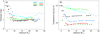 |
Fig. 3. (a) FRIS-model-derived polytropic index (Γ) with the height of the CME LE. The dashed black line represents the value of the adiabatic index (γ = 1.67). (b) FRIS-model-derived temperature (T) profile with the LE heights of the six selected CMEs. |
As discussed above, the FRIS model-derived temperature values are scaled such that each CME has a temperature of 107 K at the starting point during our observation (Fig. 3b). This will enable us to analyze the relative temperature evolution for all the selected CMEs during their evolution. The temperature for all the CMEs (except CME2 and CME6) drops rapidly at lower heights and thereafter maintains a constant value. CME2 shows a heating state (Γ < 1) throughout our model results. Thus, its temperature is not decreasing as rapidly as others. In contrast, CME4 attends a near adiabatic state at greater heights, which is reflected in its temperature profile as well. The temperature of CME4 is decreasing continuously over the observed duration.
The analysis suggests that while successive CMEs could influence the conditions in the surrounding solar wind, the thermodynamic properties, such as the evolution of polytropic index and temperature, remain notably consistent among CMEs in this study. This result implies that CMEs may inherently possess distinct thermal characteristics, potentially set at the time of their launch, regardless of minor interaction effects with nearby solar wind alterations from preceding CMEs. Interactions between multiple CMEs within a short interval are complex and depend on various factors, including the local magnetic field vector, orientation, and relative direction of each CME. For instance, CME3, CME4, and CME5 erupted within approximately four hours. CME3 and CME4, given their longitudinal separation and faster speed of CME4, could experience a side-on interaction. Our extrapolated kinematics of CME3 and CME4 show a LE interaction height of around 50 R⊙. However, taking the aspect ratio (k) value of 0.24 (Table 1) and LE height (h) of ≈30 R⊙ (Fig. 2c), the trailing edge height [ ] for CME3 is found to be ≈18.4 R⊙. As a result, CME4 begins interacting with the trailing part of CME3 at around 20 R⊙, leading to a noticeable decrease in LE acceleration beyond this height (Fig. 2b). Although CME3 and CME4 are launched in different directions, their calculated total angular width (2α + 2sin−1k) (Thernisien 2011) are 584° and 66°, respectively. Combined with the higher speed of the trailing CME4, this suggests that an interaction between CME3 and CME4 is indeed likely. A clear change in polytropic index value (Fig. 3a) is seen for CME4 beyond ≈22 R⊙, suggesting a thermal adjustment possibly due to the deceleration influence of interaction with CME3’s trailing part. In contrast, CME4 and CME5 show minimal interaction probability, given the slower initial propagation speed of CME5. The derived thermal properties of CME5 show no significant changes within our observed remote sensing heights. The likelihood of their interaction could increase if CME4 slows down after interaction with CME3 or CME5 gains acceleration after interaction with the faster following CME6. Thus, in situ measurements at 1 AU can provide more insights into the thermal properties of CME5 and all other selected CMEs at later heights.
In the forthcoming sections we analyze and disentangle the complex ICME structures using in situ measurements. Further, we derive the thermal state of the interacting ICME structures from in situ measurements to get some insights into the interaction.
3. Near-Earth in situ observations
We identified the large-scale solar wind structures in the in situ observations at 1 AU associated with the candidate CMEs of the great geomagnetic storm. Figure 4 shows the solar wind properties near Earth during the geomagnetic storm observed by the Wind (Ogilvie & Desch 1997) spacecraft at the first Lagrange (L1) point, as well as the Dst index on 10–11 May 2024. The magnetic field data (1-minute resolution), solar wind bulk speed (92-second resolution), and plasma data (92-second resolution) are obtained from the MFI (Lepping et al. 1995), SWE (Ogilvie et al. 1995), and 3DP (Lin et al. 1995) instruments on board Wind, respectively. The ground-based Dst index (1-hour resolution) is obtained from the World Data Center for Geomagnetism, Kyoto (Nose et al. 2015).
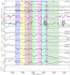 |
Fig. 4. Structures of the CMEs that drove the great geomagnetic storm on 10–11 May 2024, as measured in situ by Wind. Panels (a) and (b): Average magnetic field and its components in GSE coordinates, respectively. Panels (c) and (d): Calculated inclination angle, θ (with respect to the ecliptic plane) and azimuthal angle, ϕ (0 deg pointing to the Sun) of the magnetic field. Panels (e), (f), (g), (h), (i), and (j): Bulk solar wind speed, proton number density, proton temperature, electron number density, electron temperature, and plasma beta, respectively. Panel (k): Dst index value for the selected duration of in situ measurements. The vertical color bars in each panel show the corresponding structures, such as sheath (S), magnetic ejecta (ME), and interaction regions (IRs). The dotted regions following the leading portion within ME2 and ME4 display signatures similar to double FR structures, which may have been inherently present during the eruption or developed later due to CME-CME interaction. The shaded regions have not been overlaid on panel K as the Dst index represents the geomagnetic response and therefore does not align with the measurements from the Wind spacecraft taken at L1. |
To aid in identifying the various substructures within the complex ejecta, we estimated the inclination angle, θ (with respect to the ecliptic plane) using the magnitude of the total magnetic field (B) and the normal component of the magnetic field (Bz) as  . Since the azimuthal angle ϕ rotates in the ecliptic plane (from 0° to 360°), it is estimated using the magnetic field components Bx and By as follows:
– For Bx > 0 and By > 0, 
– For Bx < 0 and By > 0, 
– For Bx < 0 and By < 0, 
– For Bx > 0 and By < 0, 
Such an approach to estimating the inclination and azimuthal angle of the magnetic field to identify the substructures in a single CME/MC near 1 AU is followed earlier (Agarwal & Mishra 2024, 2025). The values of θ and ϕ are shown in Figs. 4b and 4c.
A sudden enhancement of magnetic field (B) and speed (V) of solar wind plasma can be observed around 16:35 UT on 10 May 2024, indicating the arrival of the shock. This shock could correspond to the CME1. The arrival of shock at the bow of the magnetosphere leads to a compression of the magnetopause, which results in a rapid increase in the Earth’s magnetic field on the day-side and is called a sudden storm commencement (SSC). The SSC can be seen in the Dst index profile (Fig. 4i) of this great geomagnetic event, where the Dst index rises to a value of around 61 nT. The SSC lasted about 2 hours before we saw a negative Dst index value.
The shock was followed by a turbulent sheath region (region S in purple shade in Fig. 4) characterized by a high value and fluctuation in magnetic field (B), rapid fluctuation in magnetic field vectors (BGSE), a rise in proton density (np), and a rise in proton temperature (Tp). The ME arrived at 19:25 UT on 10 May 2024, which we associate with CME1. This region is marked as ME1 (yellow shade) in Fig. 4. This shows a higher value of the magnetic field (B), rotation in magnetic field vectors (BGSE), decrease in proton density (np), temperature (np), and plasma beta less than unity. Following ME1, we observe a sudden change in the magnetic field vectors, θ, and ϕ. Noting the smooth rotation in the magnetic field vectors and a lower plasma beta, we attribute this to ME2. Interestingly, the LE speeds and accelerations of CME1 and CME2 are estimated to be similar at 20 R⊙ (Fig. 2). However, the preceding CME1 may have cleared the ambient medium, resulting in a lower-density region ahead of CME2, potentially reducing the drag it experiences. This enhances the likelihood of interaction between CME1 and CME2. We identified interaction regions (IRs) between MEs by analyzing in situ magnetic and plasma parameters (gray shaded regions in Fig. 4) as discussed in Mishra et al. (2015a). The IR1 between ME2 and ME3 is characterized by an interval of decrease in magnetic field, sudden rapid rotation in the magnetic field vector, enhancement in proton density, and plasma beta. As discussed in Sect. 2, CME3 has a half angle of 15° and source regions of longitude of 27° east of the Sun-Earth line, we expect a definite CME3 flank encounter at Earth ahead of CME4 and the identified region marked as ME3. Furthermore, we differentiated ME4 from ME3 based on magnetic and plasma properties, including lower proton and electron number densities, differences in magnetic field vector directions, and the θ value for ME3. We identified an IR (IR2) in between ME4 and ME5 that exhibits signatures of a decrease in the magnetic field, a sudden rapid rotation in the magnetic field vector, an increased proton temperature, and an elevated plasma beta. We observe that IR1 exhibits a noticeable increase in proton density but does not clearly show a higher proton temperature, whereas IR2 shows an increase in proton temperature without a distinct rise in proton density. The GCS model estimated a longitude of 38° west of the Sun-Earth line for CME5, suggesting a possible flank encounter at Earth. However, in situ observations of the marked region ME5 showed a smooth rotation of magnetic field vectors, lower plasma beta, and reduced proton temperature. This suggests that CME5 may have undergone a deflection toward the Sun-Earth line due to its interaction with CME6, as high-speed CMEs can realign slower CMEs toward their trajectory following an interaction. We identified an IR (IR3) in between ME5 and ME6 that is marked by rapid variations in magnetic field vectors, along with increases in density, temperature, and plasma beta.
The gray dotted regions in the trailing part of ME2 and ME4 (Fig. 4) can be attributed to interaction-driven changes. Lugaz et al. (2013) demonstrated that the relative inclination of 90° between two ejecta increases the chances of their merging to become a single structure. The GCS model estimated the tilt angle for CME2 and CME3 to be 27° and 79°, respectively. Although the relative difference in tilt is not large, the interaction with CME4 may have altered the tilt of CME3, thus enhancing the interaction between CME2 and CME3. Similarly, the tilt angles for CME4 and CME5 were estimated to be 15° and –83°, respectively, which also favors their interaction. Prior to each IR (IR1 and IR2), the preceding ME shows noticeable deformation in magnetic field orientation and an increase in plasma parameters, including np, Tp, ne, Te, and β (gray dotted regions in Fig. 4). Because of the early interaction between CME3 and CME4, the shock associated with CME4 was able to travel through CME3, and during the interaction between CME3 and CME2, the same shock further propagated through CME2. Lugaz et al. (2005, 2009) show that when the trailing shock impacts the leading ME, the dense sheath behind the trailing shock must remain between the two ME, even as the shock continues to propagate through the first ejecta. This phenomenon explains the presence of IRs between ME2 and ME3 and between ME4 and ME5, as we observe in this study. Studies utilizing numerical models (Lugaz et al. 2005; Xiong et al. 2007) can provide a more detailed understanding of the interaction effects, which is beyond the scope of this study.
Given that CMEs are magnetized plasma structures moving through the ambient solar wind, analyzing the interaction or collision of CMEs is a complex task. Several studies have examined the nature of these collisions and the subsequent changes in CME properties, such as propagation speed, expansion, and size (Temmer et al. 2014; Mishra & Srivastava 2014; Mishra et al. 2016; Shen et al. 2016). In this study, all CMEs except CME3 exhibit visible shock signatures in the coronagraphic images, leading us to expect that the faster CME with a shock will accelerate the preceding CME (Schmidt & Cargill 2004; Lugaz et al. 2005). Thus, we notice a gradual increase in speed for the whole combined ejecta in the in situ measurements. We find no shock signatures associated with each faster CME, which were identified as distinct structures within the combined ejecta at 1 AU. The CME-CME interaction well before arriving at 1 AU and shock propagation through the leading ME might be a reason for weakening the shock properties (Lugaz et al. 2005, 2009). In an overall view of the complex interacting structures, we observe that the speed of the combined structure continues to increase while overall, it gradually decreases in density and temperature. This indicates that the trailing ME continues to compress and accelerate the preceding combined structure.
3.1. Determining thermodynamics using in situ measurements
Some studies have been conducted to understand the thermodynamic behavior of CMEs by analyzing their in situ observations. However, such studies are lacking for a complex ejecta formed from several interacting CMEs. By considering the CME plasma goes through a polytropic process during its evolution, the value of the polytropic index (Γ) can describe the thermal state of plasma. The polytropic equation (Tn1 − Γ=constant) quantifies the relationship between plasma density (n) and temperature (T). Thus, by performing a linear fit to the logarithmic values of density and temperature, the Γ value can be determined. Previous studies have estimated the Γ value for ICMEs using in situ observations at distances ranging from 0.3 to 20 AU from the Sun, finding values between 1.15 and 1.33 (Liu et al. 2005, 2006). Model-derived results suggest a near-isothermal state in the region closer to the Sun, spanning 3–25 R⊙ (Khuntia et al. 2023), implying a considerable local plasma heating inside ICME. It could be possible that because of local small-scale processes for heating, such as magnetic reconnection, turbulence, and interaction with the solar wind, the different parts of a single ME or complex ejecta may not be in the same thermal state at a time. In this case, a linear fit to the whole duration for a single ejecta or a complex ejecta may not give results with good correlation coefficients (CCs). Therefore, we expect that performing the linear fit to various small intervals within a complex ejecta can give a better picture of the thermal state for individual intervals. Using a similar approach, recent studies determined the radial variation of the thermal state of solar wind (Nicolaou et al. 2014, 2020). Dayeh & Livadiotis (2022) applied this approach to analyze the statistical thermal state of various structures associated with ICMEs, revealing an adiabatic state for the pre- and post-ICME regions, while the ME exhibits a near-adiabatic heating state.
We used 92-second resolution Wind measurements for the identified complex ejecta in addition to the ambient solar wind plasma 6 hours before and after the ejecta. The pre-and post-intervals of complex ejecta are taken to compare the thermodynamics of complex ejecta with the ambient medium at that time. We used the Wind/3DP instrument observations for the plasma (both ion and electron) density and temperature, and the data were obtained from the Coordinated Data Analysis Web (CDAWeb). We selected an optimal subinterval duration of 6 data points (9.2 minutes) to fit the density and temperature variations and estimate the value of the polytropic index. We applied a linear fit between the value of log T and log n to calculate the value of the polytropic index for the subinterval, along with the corresponding Pearson CC and p-value (p). The analysis was also performed using subinterval durations ranging from 4 data points (6.13 minutes) to 10 data points (15.33 minutes), with no statistically significant variation in the results. Longer subintervals may encompass a mix of different plasma streamlines, potentially leading to lower CC values while fitting the density-temperature variations. We repeated this fitting procedure for moving subintervals with a step size of 92 seconds. By doing so, we increased the number of data points available for Γ measurements, improving the likelihood that the plasma within each subinterval corresponds to a single thermal state. Previous studies utilized different filtering techniques on solar wind plasma data to select the optimal subinterval for calculating Γ (Nicolaou et al. 2014, 2020; Dayeh & Livadiotis 2022). Our study filtered subintervals based on correlation conditions, including only those with a CC ≥ 0.8 and p ≥ 0.05. This approach ensures that the obtained gamma value accurately represents the thermal state of the entire subinterval. We did not apply the Bernoulli integral filter, which is typically used to ensure that the solar wind plasma parcel follows a single streamline. However, we consider that applying this filter is not necessary, as the CC conditions ensure that the Γ value reliably captures the thermal properties of the entire subinterval, even if the Bernoulli integral varies within the entire subinterval.
Figures 5a and 5b show the variations of the polytropic index (Γ) within the complex ejecta and within pre-and post-intervals of the complex ejecta in the solar wind medium for both electrons and ions, respectively. In each panel, we overlay the reference lines for the adiabatic index (Γ = 1.67) and isothermal index (Γ = 1) values. In each panel we plot both the reliable (orange color) and unreliable (gray color) Γ values obtained from fitting density and temperature. The reliable values correspond to a good fit of density and temperature to be accepted for further interpretation of the thermal state. Additionally, the right side of each panel shows the histogram for reliable Γ values within the complete duration of complex ejecta only. We note that the electron Γ (Γe) values show a clear distinction between the complex ejecta and ambient solar wind (pre and post-ejecta). The pre-interval of complex ejecta displays dominant Γe values of less than 1.67, suggesting heating in these regions. In contrast, most of the measured Γe values for the complex ejecta structures and post-interval are above 1.67, indicating a heat-release state. The mean and median of the occurrences of Γe values inside the complex ejecta were 2.78 and 2.59, respectively. The bottom panel shows the ion Γ (Γi) values for the complex ejecta and ambient solar wind (pre and post-intervals). There is a clear distinction for Γi values for the complex ejecta and ambient solar wind before and after. The Γi shows mostly heating signatures for pre and post-intervals of the complex ejecta. The Γi values inside the complex ejecta have a two-peak distribution, showing mixtures of thermal states. Moreover, the mean and median of Γi inside the complex ejecta were found to be 1.31 and 1.41, respectively. This suggests a predominant heating state within the ejecta and also significant occurrences of heat release.
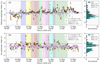 |
Fig. 5. Electron (a) and proton polytropic index (b) for the ICME structures measured using Wind data. |
Examining the thermal states of each structure within the complex ejecta reveals a trend: each subsequent ME exhibits, on average, higher Γe values than its preceding ones (Fig. 5a). This indicates that each subsequent CME in the complex ejecta (i.e., the interactions that happened later in time and thus existed for a shorter time before being observed by in situ spacecraft at 1 AU) change more intensely into heat-release states. This trend is also noticed for interacting regions IR1, IR2 and IR3. The second IR (IR2), having formed later than IR3, displays more pronounced heat-releasing states. We could not find a specific trend in Γi values for each following interacting CME, but overall, the complex ejecta shows predominantly heating signatures, with some short intervals of heat-release states.
The Γ value of a single CME (protons) has been statistically estimated to range between 1.1 and 1.3 from 0.3 to 20 AU (Liu et al. 2006), indicating significant heating during its evolution. On a larger scale, the Γ value for solar wind protons typically lies between 1.5 and 1.67, while it tends to reach higher values, around 2.7 on smaller scales (Nicolaou et al. 2020). As previously discussed, the large-scale solar wind structure we are analyzing is identified as a complex ejecta and displays signatures of past interactions between potential CMEs. The difference in the electron and proton polytropic index is unsurprising as the electrons, due to their significantly smaller mass than protons, may respond more quickly and intensely to any physical processes causing thermal perturbations.
As discussed in Sect. 2.1, the CME-CME interaction heights are estimated to be well before 1 AU. These interaction heights are approximately 144 R⊙ for CME1 and CME2, 54 R⊙ for CME3 and CME4, and 110 R⊙ for CME5 and CME6. However, it is important to note that this finding is from our simple approach, given the lack of measured kinematic information on CMEs after the coronagraphic field of view and in their post-interaction phases. This implies that establishing a one-to-one connection between CME sequences and speeds derived from remote observations with those from in situ measurements is challenging. In in situ observations, we do not find any IRs sandwiched between ME1 and ME2, nor between ME3 and ME4 (Fig. 4). Earlier studies have also noted the occasional absence or presence of such IRs between interacting CMEs in in situ observations (Mishra et al. 2015a,b). The absence of IRs between a preceding-following CME pair could be due to some characteristics of the following CME, making it less efficient in piling up ambient material and causing a smaller sheath thickness. We think that the presence or absence of IRs could also be an effect of the nature of collision between interacting CMEs; however, it is difficult to establish this because of the accurate measurements of 3D kinematics in the pre-and post-interaction phases of the CMEs.
Our analysis from remote observations shows a strong possibility of CME-CME interaction, and this is supported by the in situ measured enhanced temperature and the reduced size of MEs identified within the complex ejecta. This shows that heating and compression happen due to CME-CME interaction, as also shown in several earlier studies (Liu et al. 2012; Temmer et al. 2014; Mishra & Srivastava 2014). The derived polytropic index, particularly for electrons, shows a dominant heat-release state, which is possible if they are heated during these CME-CME interactions and later exhibit a heat-release state. In contrast, the heavier ions, being unable to find an equilibrium state post-interaction, still show a combination of ongoing heating and heat-release states at 1 AU. Therefore, the electron polytropic index further supports our inferences of CME-CME interaction from our extrapolated kinematics, and it could be a better proxy for CME-CME interaction than the proton polytropic index.
We also note that observations during the gray-dotted regions (discussed in Sect. 3) bear strong resemblances to double-FR structures in ME2 and ME4. The ϕ values indicate that among the two FRs in ME2, the second FR shown with a dotted region is westward directed, while the first FR is oriented eastward. A similar pattern is observed in ME4, where the second FR shown with a dotted region features an eastward directed FR while the first FR is westward oriented. Carefully inspecting θ values, we note that the first FR shows rotation from north to south, while the second tends to rotate from south to north in both ME2 and ME4. Thus, in ME2, the first and second FRs exhibit a north-east-south (NES) and south-west-north (SWN) orientations, respectively, while in ME4, the first and second FRs are oriented north-west-south (NWS) and south-east-north (SEN) (Bothmer & Schwenn 1998). We note that both FRs in ME2 have right-handedness, while both FRs in ME4 have left-handedness. This indicates that the handedness of double FRs within a single ME is the same. It is noted that the first FR in ME4 does not exhibit significant rotation in the magnetic field components, but there is an appreciable rotation in its leading portion. Therefore, it is clear that in situ observations of magnetic fields suggest handedness similar to double FRs. Also, the plasma parameters, including np, Tp, ne, Te, and β, show different characteristics between two FRs in both ME2 and ME4. Importantly, the density in the second FR (shown with a dotted region) is higher than the first FR in both ME2 and ME4. We believe these signatures, which resemble certain characteristics of double FRs, come from CME-CME interactions and interactions between the trailing part of the ME and the following ME. There are numerous in situ and remote observations of CMEs suggesting the existence of multiple FRs within the same CME (Ogilvie & Desch 1997; Hu et al. 2003; Marubashi & Lepping 2007; Farrugia et al. 2011; Nieves-Chinchilla et al. 2020; Hu et al. 2021; Wood et al. 2021). Osherovich et al. (2013) have provided the first observational example of the presence of a double FR in an erupting prominence and in situ measurements of an ICME. Similarly, Hu et al. (2003, 2021) also identified the presence of a double FR structure with opposite field polarities using the Grad-Shafranov reconstruction technique on observed ICMEs.
We focused on the thermal state of MEs, which shows distinct characteristics akin to double-FR structures. We note different mean values of Γe within the two FRs of ME2 (Γe = 1.9 for the first FR and 0.4 for the second) and ME4 (Γe = 3.0 for the first FR and 2.0 for the second), as shown in Fig. 5a. The lower value of the polytropic index during the second FR, with higher density, in both ME2 and ME4, indicates a weak correlation between temperature and density. In fact, the temperature and density between the first and second FRs of ME2 are oppositely correlated. In addition to plasma and magnetic field observations during ME2 and ME4, the thermal states also exhibit a resemblance with double-FR structures. Our finding is consistent with the study of Osherovich et al. (2013), which also suggests that the two FRs can exhibit distinct electron polytropic indices. We cannot rule out the possibility that these structures merely resemble double FRs but actually result solely from CME-CME interactions rather than originating as a double-FR system near the Sun. Identifying the physical processes responsible for the formation of these double FRs, particularly within this complex ejecta, is beyond the scope of this study. A detailed investigation combining remote sensing, in situ observations, and modeling of an isolated event could offer deeper insights into such structures.
3.2. Comparison of FRIS-model and in situ derived thermal states
The FRIS model-derived polytropic index (Γ) was calculated (Sect. 2.2) under a polytropic approximation for the entire CME with an average temperature, T = (Te + Tp)/2 and a number density, n = ne = np. Therefore, an effective polytropic index, which combines the electron and proton polytropic indices of the entire ME from in situ observations at 1 AU, needs to be compared with the model-derived polytropic index of the CME near the Sun. Since Te is associated with Γe and  with Γp, we can calculate the effective polytropic index Γeff as the weighted average of Γe and Γp and can be expressed as
where the weights are proportional to the temperatures of the electron and proton populations. In our study, we assumed that the mean value of estimated Γe, Γp, Te, and Tp corresponding to different chosen intervals within a ME represent the thermal state of that ME. The mean values representing the thermal state at 1 AU are listed in Table B.1. Using these mean values, we further calculated Γeff for ME1, ME2, ME3, ME4, ME5, and ME6, which are 1.77, 1.47, 0.8, 1.63, 1.26, and 1.75, respectively. ME1 and ME6 exhibit a heat-release state at 1 AU, ME2 and ME4 indicate a near-adiabatic heating state, while ME3 and ME5 display a near-isothermal heating state.
On comparing the estimates of Γeff near 1 AU with those Γ derived from the model, we find a large difference for ME1 and ME6, almost no change in ME3, ME4, and ME5, and a moderate change for ME2. Such a direct comparison based on only two-point measurements (one close to the Sun and the other at 1 AU) to understand any change in the thermal states of CMEs due to interaction could have been meaningful for only one interacting CME pair. However, in our case, there are multiple interacting CME pairs, and they are expected to undergo multiple heating and heat-release states. Therefore, a one-to-one comparison between the in situ and model-derived Γ would be extremely difficult to achieve a meaningful thermal history. Our study emphasizes that the thermodynamic evolution of interacting CMEs is complex; therefore, one needs information on the continuous thermal history of CMEs during their pre-, ongoing, and post-interaction phases for better understanding. Future studies utilizing HI observations combined with in situ observations of CMEs at distances covering their pre- and post-interaction phases would provide more insights into their ongoing thermal states.
4. Conclusions
We have identified a series of six CMEs ejected in succession from the Sun on 8–9 May 2024 that led to the great geomagnetic storm that began on 10 May 2024. Using data from SOHO/LASCO-C2, STEREO-A/COR2, and SDO/AIA, we analyzed the identified CMEs and applied the GCS model to derive their 3D kinematics and understand their interactions before arriving on Earth as a complex ejecta. Our study also focused on the thermodynamics of the selected CMEs, using both remote and in situ observations. The following points summarize the findings of our study,
-
From the measured 3D kinematics, we conclude that the potential interactions among the selected CMEs (CME1 and CME2 at 144 R⊙, CME3 and CME4 at 54 R⊙, and CME5 and CME6 at 110 R⊙) formed a complex ejecta before reaching 1 AU.
-
We also identified different MEs in the in-situ observations corresponding to near-Sun-identified CMEs and noted the signatures of the CME-CME interaction. The interacting CMEs show clear signatures of heating and compression. This suggests that CME interactions significantly influence their large-scale properties and impact space weather near Earth.
-
We identified IRs between pairs of MEs in in situ observations. This indicates that CME-CME interactions occurred as they propagated toward Earth. Additionally, we observe two ME (ME2 and ME4) that have a magnetic field, a polytropic index, and density-temperature characteristics similar to those of double-FR structures. Double-FR-like structures may have appeared due to variations in ME properties resulting from CME-CME interactions.
-
The thermal evolution of CMEs varied significantly, even before the interaction, with most CMEs transitioning to an isothermal state at higher coronal heights, while exceptions like CME4 approached an adiabatic state. The FRIS model shows that heating or heat release in the plasma depends on the CME’s propagation and expansion, with a slower expansion leading to heat release, as observed in CME4. We did not notice a difference in the CMEs’ thermodynamics in their later phase at coronal heights despite the fact that each of them was traveling in a different preconditioned medium.
-
In situ observations at 1 AU show that electrons within the interacting CMEs forming complex ejecta are in a predominant heat-release state, as indicated by their polytropic index values (Γe > 1.67). We also note that the post-interval of the complex ejecta shows a predominant heat release, while the pre-interval shows a heating state, suggesting distinct thermal processes are occurring inside and outside the interacting large-scale structures.
-
The polytropic index for ions (Γi) inside the complex ejecta has a significant bimodal distribution, with a predominant heating state with some intervals of heat-release states, which is unlike the electron polytropic index. The difference in the electron and proton polytropic index could be due to a more gradual thermal evolution of protons than electrons in interacting CMEs, and the thermal state may depend on the amount of time they spent post-interaction.
Overall, the combination of thermal and kinematic analyses offers valuable insights into the evolution of the interacting CMEs. Pairs of interacting CMEs caused the great geomagnetic storm. While geo-effectiveness was not the primary focus of the study; it highlights the broader implications of such interactions in influencing CME plasma properties and their potential geo-effectiveness. Our study, which focused on the thermodynamic evolution of the CMEs, confirms the CME-CME interactions from both remote and in situ observations. We plan to use heliospheric imaging observations to provide further insights into their pre- and post-interaction behaviors. Detecting properties of different substructures, such as IRs and double FRs within the complex ejecta, requires further in-depth investigations; remote and in situ observations are needed to better examine their roles in causing such a rare great geomagnetic storm.
Acknowledgments
We appreciate the anonymous referee’s valuable comments, insightful questions, and constructive suggestions that greatly improved this manuscript.
References
- Agarwal, A., & Mishra, W. 2024, MNRAS, 534, 2458 [Google Scholar]
- Agarwal, A., & Mishra, W. 2025, ApJ, 982, 183 [Google Scholar]
- Boteler, D. H. 2019, Space Weather, 17, 1427 [CrossRef] [Google Scholar]
- Bothmer, V., & Schwenn, R. 1998, Ann. Geophys., 16, 1 [Google Scholar]
- Brueckner, G. E., Howard, R. A., Koomen, M. J., et al. 1995, Sol. Phys., 162, 357 [NASA ADS] [CrossRef] [Google Scholar]
- Dayeh, M. A., & Livadiotis, G. 2022, ApJ, 941, L26 [NASA ADS] [CrossRef] [Google Scholar]
- Desai, R. T., Zhang, H., Davies, E. E., et al. 2020, Sol. Phys., 295, 130 [NASA ADS] [CrossRef] [Google Scholar]
- Domingo, V., Fleck, B., & Poland, A. I. 1995, Sol. Phys., 162, 1 [Google Scholar]
- Dungey, J. W. 1961, Phys. Rev. Lett., 6, 47 [NASA ADS] [CrossRef] [Google Scholar]
- Farrugia, C. J., Berdichevsky, D. B., Möstl, C., et al. 2011, J. Atmos. Sol.-Terr. Phys., 73, 1254 [Google Scholar]
- Gonzalez, W. D., Joselyn, J. A., Kamide, Y., et al. 1994, J. Geophys. Res., 99, 5771 [NASA ADS] [CrossRef] [Google Scholar]
- Gonzalez, W. D., Echer, E., Clúa de Gonzalez, A. L., Tsurutani, B. T., & Lakhina, G. S. 2011, J. Atmos. Sol.-Terr. Phys., 73, 1447 [Google Scholar]
- Gonzalez-Esparza, J. A., Sanchez-Garcia, E., Sergeeva, M., et al. 2024, Space Weather, 22, 2024SW004111 [Google Scholar]
- Gopalswamy, N., Lara, A., Lepping, R. P., et al. 2000, Geophys. Res. Lett., 27, 145 [NASA ADS] [CrossRef] [Google Scholar]
- Gopalswamy, N., Yashiro, S., Liu, Y., et al. 2005, J. Geophys. Res. (Space Phys.), 110, A09S15 [Google Scholar]
- Hajra, R., Tsurutani, B. T., Lakhina, G. S., Lu, Q., & Du, A. 2024, ApJ, 974, 264 [Google Scholar]
- Hayakawa, H., Ebihara, Y., Mishev, A., et al. 2025, ApJ, 979, 49 [Google Scholar]
- Howard, R. A., Moses, J. D., Vourlidas, A., et al. 2008, Space Sci. Rev., 136, 67 [NASA ADS] [CrossRef] [Google Scholar]
- Hu, Q., Smith, C. W., Ness, N. F., & Skoug, R. M. 2003, Geophys. Res. Lett., 30, 1385 [Google Scholar]
- Hu, Q., He, W., Qiu, J., Vourlidas, A., & Zhu, C. 2021, Geophys. Res. Lett., 48, e90630 [NASA ADS] [Google Scholar]
- Hundhausen, A. J., Sawyer, C. B., House, L., Illing, R. M. E., & Wagner, W. J. 1984, J. Geophys. Res., 89, 2639 [NASA ADS] [CrossRef] [Google Scholar]
- Jain, A., Trivedi, R., Jain, S., & Choudhary, R. K. 2025, Adv. Space Res., 75, 953 [Google Scholar]
- Kaiser, M. L., Kucera, T. A., Davila, J. M., et al. 2008, Space Sci. Rev., 136, 5 [Google Scholar]
- Khuntia, S., Mishra, W., Mishra, S. K., et al. 2023, ApJ, 958, 92 [Google Scholar]
- Khuntia, S., Mishra, W., Wang, Y., et al. 2024, MNRAS, 535, 2585 [Google Scholar]
- Kilpua, E., Koskinen, H. E. J., & Pulkkinen, T. I. 2017, Liv. Rev. Sol. Phys., 14, 5 [Google Scholar]
- Koehn, G. J., Desai, R. T., Davies, E. E., et al. 2022, ApJ, 941, 139 [NASA ADS] [CrossRef] [Google Scholar]
- Lazzús, J. A., & Salfate, I. 2024, J. Atmos. Sol.-Terr. Phys., 261, 106304 [Google Scholar]
- Lemen, J. R., Title, A. M., Akin, D. J., et al. 2012, Sol. Phys., 275, 17 [Google Scholar]
- Lepping, R. P., Acũna, M. H., Burlaga, L. F., et al. 1995, Space Sci. Rev., 71, 207 [Google Scholar]
- Lin, R. P., Anderson, K. A., Ashford, S., et al. 1995, Space Sci. Rev., 71, 125 [CrossRef] [Google Scholar]
- Liu, Y., Richardson, J. D., & Belcher, J. W. 2005, Planet. Space Sci., 53, 3 [Google Scholar]
- Liu, Y., Richardson, J. D., Belcher, J. W., Kasper, J. C., & Elliott, H. A. 2006, J. Geophys. Res. (Space Phys.), 111, A01102 [Google Scholar]
- Liu, Y., Thernisien, A., Luhmann, J. G., et al. 2010, ApJ, 722, 1762 [Google Scholar]
- Liu, Y. D., Luhmann, J. G., Möstl, C., et al. 2012, ApJ, 746, L15 [NASA ADS] [CrossRef] [Google Scholar]
- Liu, Y. D., Luhmann, J. G., Kajdič, P., et al. 2014, Nat. Commun., 5, 3481 [NASA ADS] [Google Scholar]
- Liu, Y. D., Hu, H., Zhao, X., Chen, C., & Wang, R. 2024, ApJ, 974, L8 [NASA ADS] [CrossRef] [Google Scholar]
- Lugaz, N., & Farrugia, C. J. 2014, Geophys. Res. Lett., 41, 769 [Google Scholar]
- Lugaz, N., Manchester, I., W. B., & Gombosi, T. I. 2005, ApJ, 634, 651 [NASA ADS] [CrossRef] [Google Scholar]
- Lugaz, N., Vourlidas, A., & Roussev, I. I. 2009, Ann. Geophys., 27, 3479 [Google Scholar]
- Lugaz, N., Farrugia, C. J., Manchester, I., W. B., & Schwadron, N. 2013, ApJ, 778, 20 [NASA ADS] [CrossRef] [Google Scholar]
- Lugaz, N., Temmer, M., Wang, Y., & Farrugia, C. J. 2017, Sol. Phys., 292, 64 [Google Scholar]
- Marubashi, K., & Lepping, R. P. 2007, Ann. Geophys., 25, 2453 [Google Scholar]
- Meng, X., Tsurutani, B. T., & Mannucci, A. J. 2019, J. Geophys. Res. (Space Phys.), 124, 3926 [Google Scholar]
- Mishra, W., & Srivastava, N. 2014, ApJ, 794, 64 [NASA ADS] [CrossRef] [Google Scholar]
- Mishra, W., & Teriaca, L. 2023, J. Astrophys. Astron., 44, 20 [NASA ADS] [CrossRef] [Google Scholar]
- Mishra, W., & Wang, Y. 2018, ApJ, 865, 50 [NASA ADS] [CrossRef] [Google Scholar]
- Mishra, W., Srivastava, N., & Chakrabarty, D. 2015a, Sol. Phys., 290, 527 [Google Scholar]
- Mishra, W., Srivastava, N., & Singh, T. 2015b, J. Geophys. Res. (Space Phys.), 120, 221 [Google Scholar]
- Mishra, W., Wang, Y., & Srivastava, N. 2016, ApJ, 831, 99 [NASA ADS] [CrossRef] [Google Scholar]
- Mishra, W., Wang, Y., Srivastava, N., & Shen, C. 2017, ApJS, 232, 5 [NASA ADS] [CrossRef] [Google Scholar]
- Mishra, W., Wang, Y., Teriaca, L., Zhang, J., & Chi, Y. 2020, Front. Astron. Space Sci., 7, 1 [NASA ADS] [CrossRef] [Google Scholar]
- Mishra, W., Doshi, U., & Srivastava, N. 2021a, Front. Astron. Space Sci., 8, 142 [NASA ADS] [CrossRef] [Google Scholar]
- Mishra, W., Dave, K., Srivastava, N., & Teriaca, L. 2021b, MNRAS, 506, 1186 [Google Scholar]
- Mishra, W., Sahani, P. S., Khuntia, S., & Chakrabarty, D. 2024, MNRAS, 530, 3171 [Google Scholar]
- Nicolaou, G., Livadiotis, G., & Moussas, X. 2014, Sol. Phys., 289, 1371 [NASA ADS] [CrossRef] [Google Scholar]
- Nicolaou, G., Livadiotis, G., Wicks, R. T., Verscharen, D., & Maruca, B. A. 2020, ApJ, 901, 26 [CrossRef] [Google Scholar]
- Nieves-Chinchilla, T., Szabo, A., Korreck, K. E., et al. 2020, ApJS, 246, 63 [Google Scholar]
- Nose, M., Iyemori, T., Sugiura, M., & Kamei, T. 2015, World Data Center for Geomagnetism (Geomagnetic Dst index: Kyoto) [Google Scholar]
- Ogilvie, K. W., & Desch, M. D. 1997, Adv. Space Res., 20, 559 [Google Scholar]
- Ogilvie, K. W., Chornay, D. J., Fritzenreiter, R. J., et al. 1995, Space Sci. Rev., 71, 55 [Google Scholar]
- Osherovich, V., Fainberg, J., & Webb, A. 2013, Sol. Phys., 284, 261 [Google Scholar]
- Parker, W. E., & Linares, R. 2024, J. Spacecraft Rockets, 61, 1412 [Google Scholar]
- Pesnell, W. D., Thompson, B. J., & Chamberlin, P. C. 2012, Sol. Phys., 275, 3 [Google Scholar]
- Pulkkinen, T. 2007, Liv. Rev. Sol. Phys., 4, 1 [Google Scholar]
- Richardson, I. G., & Cane, H. V. 2010, Sol. Phys., 264, 189 [NASA ADS] [CrossRef] [Google Scholar]
- Schmidt, J., & Cargill, P. 2004, Ann. Geophys., 22, 2245 [Google Scholar]
- Scolini, C., Chané, E., Temmer, M., et al. 2020, ApJS, 247, 21 [Google Scholar]
- Shen, C., Wang, Y., Wang, S., et al. 2012, Nature, 8, 923 [NASA ADS] [Google Scholar]
- Shen, F., Wang, Y., Shen, C., & Feng, X. 2016, Scient. Rep., 6, 19576 [Google Scholar]
- Spogli, L., Alberti, T., Bagiacchi, P., et al. 2024, Ann. Geophys., 67, PA218 [CrossRef] [Google Scholar]
- Srivastava, N., Mathew, S. K., Louis, R. E., & Wiegelmann, T. 2009, J. Geophys. Res. (Space Phys.), 114, A03107 [Google Scholar]
- Temmer, M., Veronig, A. M., Kontar, E. P., Krucker, S., & Vršnak, B. 2010, ApJ, 712, 1410 [NASA ADS] [CrossRef] [Google Scholar]
- Temmer, M., Veronig, A. M., Peinhart, V., & Vršnak, B. 2014, ApJ, 785, 85 [NASA ADS] [CrossRef] [Google Scholar]
- Temmer, M., Scolini, C., Richardson, I. G., et al. 2023, Advances in Space Research [Google Scholar]
- Thernisien, A. 2011, ApJS, 194, 33 [Google Scholar]
- Thernisien, A. F. R., Howard, R. A., & Vourlidas, A. 2006, ApJ, 652, 763 [Google Scholar]
- Thernisien, A., Vourlidas, A., & Howard, R. A. 2009, Sol. Phys., 256, 111 [Google Scholar]
- Tsurutani, B. T., Smith, E. J., Gonzalez, W. D., Tang, F., & Akasofu, S. I. 1988, J. Geophys. Res., 93, 8519 [NASA ADS] [CrossRef] [Google Scholar]
- Vršnak, B., & Žic, T. 2007, A&A, 472, 937 [NASA ADS] [CrossRef] [EDP Sciences] [Google Scholar]
- Wang, Y. M., Ye, P. Z., Wang, S., & Xue, X. H. 2003, Geophys. Res. Lett., 30, 1700 [Google Scholar]
- Wang, Y., Wang, B., Shen, C., Shen, F., & Lugaz, N. 2014, J. Geophys. Res. (Space Phys.), 119, 5117 [NASA ADS] [CrossRef] [Google Scholar]
- Webb, D. F., & Howard, T. A. 2012, Liv. Rev. Sol. Phys., 9, 3 [Google Scholar]
- Weiler, E., Möstl, C., Davies, E. E., et al. 2025, Space Weather, 23, e2024SW004260 [Google Scholar]
- Wood, B. E., Braga, C. R., & Vourlidas, A. 2021, ApJ, 922, 234 [NASA ADS] [CrossRef] [Google Scholar]
- Xiong, M., Zheng, H., Wu, S. T., Wang, Y., & Wang, S. 2007, J. Geophys. Res. (Space Phys.), 112, A11103 [Google Scholar]
- Yashiro, S., Gopalswamy, N., Michalek, G., et al. 2004, J. Geophys. Res. (Space Phys.), 109, 7105 [CrossRef] [Google Scholar]
- Yermolaev, Y. I., Zelenyi, L. M., Kuznetsov, V. D., et al. 2008, J. Atmos. Sol.-Terres. Phys., 70, 334 [Google Scholar]
- Zhang, J., Dere, K. P., Howard, R. A., & Vourlidas, A. 2004, ApJ, 604, 420 [NASA ADS] [CrossRef] [Google Scholar]
Appendix A: The FRIS model-fitting errors
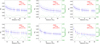 |
Fig. A.1. Model-fitting errors for the selected fast CMEs. Blue dots show the left-hand side of Eq. (1), the dashed red line the right-hand side of Eq. (1) from Khuntia et al. (2023), and the green line the relative fitting errors. MPE stands for the mean percentage error. |
Appendix B: Mean values of in situ plasma parameters
Mean values of plasma parameters for different MEs and the calculated effective polytropic index (Γeff) from in situ measurements at 1 AU.
All Tables
Mean values of plasma parameters for different MEs and the calculated effective polytropic index (Γeff) from in situ measurements at 1 AU.
All Figures
|
Fig. 1. GCS-model-fitted Earth-impacting CMEs responsible for the great event on 10 May 2024. Top panels: Running-difference imaging observations of CMEs from SOHO/LASCO-C2 and STEREO-A/SECCHI-COR2. Bottom panels: Fitted GCS model overlaid as the yellow wire frame. |
| In the text | |
|
Fig. 2. Propagation speed (a) and acceleration (b) of LE of the selected CMEs derived from the GCS-model-fitted 3D LE heights. (c) Height-time profiles of the CMEs assuming no acceleration (solid line) and some value of a constant average deceleration (dashed line). The color-filled circles indicate the first possible CME-CME interaction height. The initial dots show the GCS-fitted heights for the CMEs. We include only every other data point for the GCS-fitted heights for the sake of clarity. |
| In the text | |
|
Fig. 3. (a) FRIS-model-derived polytropic index (Γ) with the height of the CME LE. The dashed black line represents the value of the adiabatic index (γ = 1.67). (b) FRIS-model-derived temperature (T) profile with the LE heights of the six selected CMEs. |
| In the text | |
|
Fig. 4. Structures of the CMEs that drove the great geomagnetic storm on 10–11 May 2024, as measured in situ by Wind. Panels (a) and (b): Average magnetic field and its components in GSE coordinates, respectively. Panels (c) and (d): Calculated inclination angle, θ (with respect to the ecliptic plane) and azimuthal angle, ϕ (0 deg pointing to the Sun) of the magnetic field. Panels (e), (f), (g), (h), (i), and (j): Bulk solar wind speed, proton number density, proton temperature, electron number density, electron temperature, and plasma beta, respectively. Panel (k): Dst index value for the selected duration of in situ measurements. The vertical color bars in each panel show the corresponding structures, such as sheath (S), magnetic ejecta (ME), and interaction regions (IRs). The dotted regions following the leading portion within ME2 and ME4 display signatures similar to double FR structures, which may have been inherently present during the eruption or developed later due to CME-CME interaction. The shaded regions have not been overlaid on panel K as the Dst index represents the geomagnetic response and therefore does not align with the measurements from the Wind spacecraft taken at L1. |
| In the text | |
|
Fig. 5. Electron (a) and proton polytropic index (b) for the ICME structures measured using Wind data. |
| In the text | |
|
Fig. A.1. Model-fitting errors for the selected fast CMEs. Blue dots show the left-hand side of Eq. (1), the dashed red line the right-hand side of Eq. (1) from Khuntia et al. (2023), and the green line the relative fitting errors. MPE stands for the mean percentage error. |
| In the text | |
Current usage metrics show cumulative count of Article Views (full-text article views including HTML views, PDF and ePub downloads, according to the available data) and Abstracts Views on Vision4Press platform.
Data correspond to usage on the plateform after 2015. The current usage metrics is available 48-96 hours after online publication and is updated daily on week days.
Initial download of the metrics may take a while.