| Issue |
A&A
Volume 686, June 2024
|
|
|---|---|---|
| Article Number | L10 | |
| Number of page(s) | 8 | |
| Section | Letters to the Editor | |
| DOI | https://doi.org/10.1051/0004-6361/202450217 | |
| Published online | 04 June 2024 | |
Letter to the Editor
Proton polytropic behavior of periodic density structures in the solar wind
1
NASA-Goddard Space Flight Center, Greenbelt, MD, USA
e-mail: ckatsavrias@gmail.com
2
Department of Physics, National and Kapodistrian University of Athens, Athens, Greece
3
Department of Space and Climate Physics, Mullard Space Science Laboratory, University College London, Dorking, Surrey RH5 6NT, UK
4
Physics Department, The Catholic University of America, Washington, DC, USA
5
Space Applications and Research Consultancy (SPARC), Athens, Greece
6
Princeton University, Princeton, NJ 08544, USA
Received:
2
April
2024
Accepted:
20
May
2024
Context. In recent years, mesoscales have gained scientific interest because they have been determined to be important in a broad range of phenomena throughout heliophysics. The solar wind mesoscale structures include periodic density structures (PDSs), which are quasi-periodic increases in the density of the solar wind that range from a few minutes to a few hours. These structures have been extensively observed in remote-sensing observations of the solar corona and in in situ observations out to 1 AU, where they manifest as radial length scales greater than or equal to the size of the Earth’s dayside magnetosphere, that is, from tens to hundreds of Earth radii (RE). While the precise mechanisms that form PDSs are still debated, recent studies confirmed that most PDSs are of solar origin and do not form through dynamics during their propagation in the interplanetary space.
Aims. We further investigate the origin of PDSs by exploring the thermodynamic signature of these structures. To do this, we estimate the values of the effective polytropic index (Y) and the entropy of protons, which in turn are compared with the corresponding values found for the solar wind.
Methods. We used an extensive list of PDS events spanning more than two solar cycles of Wind measurements (the entire Wind dataset from 1995 to 2022) to investigate the thermodynamic signatures of PDSs. With the use of wavelet methods, we classified these PDSs as coherent or incoherent, based on the shared periodic behavior between proton density and alpha-to-proton ratio, and we derive the proton polytropic index.
Results. Our results indicate that the coherent PDSs exhibit lower Y values (Ῡ≈1.54) on average and a higher entropy than the values in the entire Wind dataset (Ῡ≈1.79), but also exhibit similarities with the magnetic cloud of an interplanetary coronal mass ejection. In contrast, incoherent PDSs exhibit the same Y values as those of the entire Wind dataset.
Key words: Sun: corona / Sun: heliosphere / solar wind
© The Authors 2024
 Open Access article, published by EDP Sciences, under the terms of the Creative Commons Attribution License (https://creativecommons.org/licenses/by/4.0), which permits unrestricted use, distribution, and reproduction in any medium, provided the original work is properly cited.
This article is published in open access under the Subscribe to Open model. Subscribe to A&A to support open access publication.
1. Introduction
In the solar wind, mesoscale structures are defined as structures that are larger than kinetic physics, but smaller than global structures such as interplanetary coronal mass ejections (ICMEs). At 1 AU, this corresponds to scale sizes ranging from a few tens to several thousand megameters (Viall et al. 2021). A subset of these mesoscales consists of quasi-periodic density structures (PDSs), which are a particular constituent of the ambient solar wind (Kepko et al. 2020). In in situ and remote-sensing observations, the PDSs reach frequencies between 0.1 and 5 mHz and are not waves, but rather represent periodic spatial intervals of enhanced proton density that are entrained in the solar wind flow (Viall et al. 2008). These structures can impact global magnetospheric and radiation belt dynamics through pressure enhancements in the solar wind (Viall et al. 2009a; Kepko & Viall 2019; Di Matteo et al. 2022). Therefore, it is highly important to understand their origin and occurrence rate.
Even though the precise generation mechanisms of PDSs are still debated, several studies have confirmed their solar origin using remote-sensing observations of the Sun (Alzate et al. 2021; Ventura et al. 2023). Especially low-frequency (< 1 mHz) PDSs have been observed as density blobs in the solar atmosphere in coronagraph observations from the COR2 instrument onboard the Solar TErrestrial RElations Observatory (STEREO) down to 2.5 solar radii (Viall & Vourlidas 2015; DeForest et al. 2018). Furthermore, in situ observations, from 0.3 to 1.0 AU (Di Matteo et al. 2019; Kepko et al. 2024), have also confirmed solar origin theories involving magnetic reconnection and interchange reconnection in the solar corona (Antiochos et al. 2011; Higginson & Lynch 2018). Using magneto-hydrodynamics (MHD) simulations, Réville et al. (2020) showed that the low-frequency PDSs may result from the periodic release of flux ropes from the tip of helmet streamers as a result of the tearing instability (Poirier et al. 2023). Interestingly, in situ measurements have also associated PDSs with small flux ropes (Kepko et al. 2016; Di Matteo et al. 2019; Lavraud et al. 2020). Finally, a PDS population might also have formed via solar wind dynamic processes (Verscharen et al. 2019; Viall et al. 2021).
A way to distinguish between the various generation mechanisms is the elemental composition, that is, the charge-state ratios or relative abundances of different elements, which are frozen in to the solar wind flow and do not evolve during their propagation. Studies of magnetic connectivity and in situ compositional changes associated with PDSs confirmed that PDSs are formed deep in the solar corona, and they are likely associated with the release of closed plasma into the solar wind (Kepko et al. 2016; Gershkovich et al. 2022, 2023).
In this work, we follow a novel approach by investigating the proton thermodynamic properties of PDSs using an estimation of the polytropic state. The polytropic behavior is the macroscopic relation between plasma moments (density, n, versus pressure, P, or temperature, T) that describes the transition of a plasma species from one state to another under constant specific heat (Parker 1963; Chandrasekhar 1957) and isotropic temperature,
where the polytropic index γ is characteristic for individual plasma streamlines. It may vary for different plasma species and within different plasma regimes, and thus, it may indicate different thermodynamical states (Kartalev et al. 2006; Nicolaou et al. 2014; Livadiotis 2016; Dialynas et al. 2018).
The polytropic relation is directly related to plasma thermodynamics because it determines the amount of heat that is supplied or emitted from the plasma during a specific process. Recently, the polytropic index was used to describe the dynamics of ICMEs (Dayeh & Livadiotis 2022). Dayeh et al. measured the turbulent heating rates in ICME plasma by showing that they exhibit a lower average proton polytropic index than its adiabatic value, which resulted in a positive entropic gradient. Here, we apply for the first time, to our knowledge, a similar method in order to determine the heating processes governing protons in PDSs. We use a list of solar wind PDSs that were detected during more than two solar cycles in data from the Wind spacecraft. The manuscript is organized as follows: Sect. 2 describes the particular technique we used to identify and classify PDSs, as well as the method for deriving the proton polytropic index. In Sect. 3 we present the results of the polytropic index values and distributions, and we compare them with those of the entire Wind dataset. Finally, we discuss our results and summarize our conclusions in Sect. 4.
2. Data and event list of periodic density structures
We used solar wind measurements from the Solar Wind Experiment instrument (SWE; Ogilvie et al. 1995) on board the Wind spacecraft near L1 with a resolution of ≈98 s (the resolution varied over the course of the mission). We considered the solar wind proton (np) and alpha (nα) number density, as well as their ratio (nα/np). Their respective standard deviation was obtained through the bi-Maxwellian approach of Kasper et al. (2006). Further, measurements of the proton thermal speed as well as solar wind speed were considered, while the solar wind magnetic field was obtained from the Magnetic Field Instrument (MFI; Lepping et al. 1995). The data we used span the period 1995–2022.
2.1. Identification of periodic density structures in wind proton density data
To identify PDS in wind np time series, we followed the spectral analysis procedure developed by Di Matteo et al. (2021) that is based on the multitaper method (MTM; Thomson 1982). In particular, we estimated the adaptive MTM power spectral density over linearly detrended six-hour intervals. Then, we identified periodic variations in the time series at frequency values at which both the normalized spectrum and an additional statistical test for phase coherence (harmonic F-test) exceed the corresponding 90% confidence threshold. The combination of the MTM and harmonic F-test is a robust approach that has been extensively tested and employed to identify PDSs in in situ measurements (Viall et al. 2008, 2009a,b; Di Matteo et al. 2019; Kepko et al. 2020, 2024) and in remote-sensing observations (Viall et al. 2010; Viall & Vourlidas 2015). Here, we implement the more recent version of this approach (SPD_MTM; Di Matteo et al. 2020, see also Appendix A.1), which was employed in earlier investigations of PDSs in solar wind plasma and composition measurements (Di Matteo et al. 2022; Gershkovich et al. 2022, 2023).
Based on this analysis, we identified 1862 PDS events with frequencies in the range of 0.2–0.9 mHz. We note that the upper frequency limit was selected in order to have enough data points to derive the polytropic index through the fitting process, without mixing consecutive PDSs.
2.2. Classification of the identified periodic density structure events
2.2.1. Duration of the periodic density structure events
In order to determine the exact duration of each PDS event, we used the continuous wavelet transform (CWT; Torrence & Compo 1998) and the Morlet wavelet (Morlet et al. 1982) as mother wavelet, following Katsavrias et al. (2012). We calculated the wavelet power spectral density of the proton density time series in each of the 1862 six-hour intervals identified via the MTM method. Then, we isolated the time periods in which the power at the corresponding PDS frequency exceeded the 75th percentile of the power during the six-hour interval (again at the same frequency as identified with the MTM method). Finally, in order to avoid any dubious detections, we required the duration of each PDS to be at least twice its period. This criterion produced a list of 1176 PDS events with frequencies in the range of 0.2–0.9 mHz.
2.2.2. Classification of periodic density structure events in terms of solar corona origin
Next, we used the cross-wavelet transform and the wavelet coherence (henceforward, XWT and WTC, respectively) between the np and nα/np time series, following Di Matteo et al. (2024) (see also Appendix A.3 for more details).
We classified each of the 1,176 PDS events into three categories as follows:
-
In coherent events, the common power in the XWT between np and nα/np exceeds the 75th percentile of the common power in the six-hour interval at the corresponding frequency, and at the same time, the corresponding WTC is higher than 0.7.
-
In low-coherence events, the common power in the XWT between np and nα/np exceeds the 75th percentile of the common power in the six-hour interval at the corresponding frequency, but the corresponding WTC is lower than 0.7.
-
In incoherent events, the common power in the XWT between np and nα/np is lower than the 75th quantile of the common power in the six-hour interval at the corresponding frequency.
This classification resulted in 330 coherent, 505 low-coherence, and 341 incoherent events. Figure 1 shows an example of a coherent and an incoherent event.
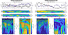 |
Fig. 1. Example of a coherent (left panels) and incoherent (right panels) event. From top to bottom: time series of np and nα/np (black and blue lines, respectively), wavelet spectrum for np, wavelet power spectrum for nα/np, cross-wavelet spectrum, and wavelet coherence. The vertical dashed red lines correspond to the times at whic the wavelet power, at the corresponding PDS frequency exceeds the 75th quantile of the power of the entire six-hour interval. The solid black lines in all spectra depict the cone of influence, where edge effects in the processing become important. The arrows in XWT and WTC point to the phase relation of the two data series in time-frequency space: (1) Arrows pointing to the right indicate in-phase behavior, and (2) arrows pointing to the left indicate antiphase behavior. |
3. Calculation of the polytropic index
The first step for the calculation of γ is to analyze sufficiently short subintervals in order to minimize the possibility of mixing measurements of different streamlines (Kartalev et al. 2006; Livadiotis 2018; Nicolaou & Livadiotis 2019). We used a sliding window of ≈10 min, which corresponds to half of the maximum period of PDSs in our list. Furthermore, in order to increase our statistics, we upsampled Wind data to 49 s (half of the nominal resolution to avoid potential artifacts) using linear interpolation, thus having 12 points per moving window. Finally, we required that each window contained nine valid points at least.
The second step was to consider the logarithm of Eq. (1) for solar wind protons,

and to perform a repeated median regression (Siegel 1982), which is a variation of the Theil-Sen estimator. In detail, for each sample point (xi, yi), the median mi of the slopes (yj − yi)/(xj − xi) of the lines through that point is derived. Then, the overall estimator is the median of these medians. We chose to use the repeated median regression over the more common least-squares linear fit because it offers a more robust option for our purposes. For the small number of data points per window (12) on which the fits were performed, even a singular outlier can detrimentally impact a least-squares fit, while the median regression is much less sensitive to outliers. It thus is optimally suited for evaluating γ.
As a third step, we examined the stability of Bernoulli’s integral by requiring the variance over the mean to be lower than 2%. This condition is particularly important because it enhances the possibility that the analyzed subintervals correspond to individual streamlines, where the polytropic relation is valid (Kartalev et al. 2006). For the plasma near 1 AU, Bernoulli’s integral can be estimated from the solar wind parameters following Livadiotis (2016)
where VSW is the proton bulk speed, ρ is the proton mass density, and B is the interplanetary magnetic field strength, while P corresponds to the proton pressure alone.
Finally, for each window satisfying these criteria, we further filtered our results by requiring that
-
The Pearson correlation coefficient of the regressed versus the measured data points was higher than 0.8, and that
-
The special polytropic index (vinv), which corresponds to the inverse spectrum regression (see also Nicolaou et al. 2019; Livadiotis 2019), must differ by no more than 0.3,
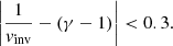
An example of a valid derivation of γ is shown in Fig. 2.
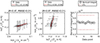 |
Fig. 2. Example of a valid derivation of γ satisfying all the criteria set for this study. The left and middle panels show the cross plots of ln(Tp) vs. ln(np) and ln(np) vs. ln(Tp), respectively, with the Wind data shown as black circles (and the corresponding standard deviation with error bars) and the regressed values as the solid red line. The right panel shows Bernoulli’s integral estimate for the same window (black circles) along with the 2% limit (dashed red lines). |
4. Results
Figure 3 shows the histograms of the derived (filtered) polytropic indices for (left panel) the entire Wind dataset spanning 1995–2022, (middle panel) the 341 incoherent PDS events, and (right panel) the 330 coherent PDS events. We note that there is a sharp dip in the histograms of the filtered values for γ ≈ 1, which corresponds to isothermal plasma. This is due to the filtering of the Pearson coefficient and the inverse polytropic index. When one parameter varies significantly for these intervals while the other is nearly constant, the regression process fails because it cannot determine a slope close to zero (for the forward regression) or close to infinity (for the inverse regression). This further means that even though the derived γs were derived using the best fits, the filtering also excluded real near-isothermal values (see also Nicolaou et al. 2014, and discussion therein).
 |
Fig. 3. Distributions of γ for (left panel) the entire Wind dataset spanning 1995–2022, (middle panel) the 341 incoherent PDS events, and (right panel) the 330 coherent PDS events. The solid red lines correspond to the best-fit κ-Gaussian distribution using a weighted nonlinear fit. |
Therefore, in order to determine the average γ value of the distribution, we performed a weighted fitting focusing on its tails rather than its most frequent value. Following Livadiotis & McComas (2011) and Nicolaou et al. (2014), we fit a κ-Gaussian distribution given by
![$$ \begin{aligned} f(\gamma ,\overline{\gamma },\kappa _{0},\sigma ) \propto \left[ 1 + \frac{\left( \gamma - \overline{\gamma }\right)^{2}}{\kappa _{0}\cdot \sigma ^{2}} \right]^{-\kappa _{0}-3/2} . \end{aligned} $$](/articles/aa/full_html/2024/06/aa50217-24/aa50217-24-eq8.gif)
The weighted κ-Gaussian fit in the case of the entire Wind dataset (solid red line in the left panel of Fig. 3) resulted in a  . This agrees with the results of Nicolaou et al. (2014) and Livadiotis (2018), who estimated
  and ≈1.86, respectively. We note that although we used a slightly different method, different criteria, and a significantly larger sample (more than two solar cycles of data), these differences in the polytropic index are negligible.
Next, using the solar wind  as benchmark, we compared the results for the coherent (right panel of Fig. 3) and incoherent (middle panel of Fig. 3) PDS events. As shown, the incoherent events exhibit the same
  (even though with higher uncertainty) as that of the entire Wind dataset. In contrast, the coherent events exhibit a slightly subadiabatic
  . The
. The  for the low-coherence events (shown in Fig. B.1) is ≈1.62. This is expected because we used a strict but arbitrary threshold for the coherence level (i.e., 0.7). Therefore, the low-coherence category may include events that indeed exhibit oscillations at the same frequency between np and nα/np, as a result of a common physical mechanism, but they simply did not pass our thresholds. Consequently, in order to avoid any confusion, we do not include the low-coherence events in the following discussion.
Last, we examined the distribution of the PDS events with respect to the solar wind density and velocity, as well as to the solar cycle phase, to rule out any systematical physical effects that might arise from the classification process and might affect our results. As shown in Nicolaou & Livadiotis (2019), the polytropic index of the solar wind varies little on an annual basis depending on the year of the solar cycle phase. In our case, the annual occurrences of coherent and incoherent PDS events (see Fig. B.2) are quite similar throughout the years we investigated. Furthermore, Livadiotis (2018) showed that even though the polytropic index of the solar wind proton plasma (near 1 AU) can be considered independent of the plasma flow speed on an annual basis, most of the fluctuations of the polytropic index appear in the fast solar wind. Figure B.3 in the appendix shows that the distributions of coherent and incoherent events with respect to the median and maximum speed, as well as the median and maximum density, exhibit a quite similar pattern. Therefore, we can safely assume that the derivation of γ for the two PDS classes is statistically significant and not biased by the sample used.
5. Discussion and conclusions
Using more than two solar cycles of Wind measurements (1995–2022), we have identified a list of 1176 low-frequency PDS events (< 1 mHz). These PDS events were further classified into two categories: a) 330 coherent events, where the corresponding frequency was detected in both np and nα/np with high coherence, and b) 341 incoherent events, where the corresponding frequency where detected in np alone. These two PDS classes are shown to be in a different thermodynamical state in terms of their polytropic behavior. Specifically, incoherent PDSs exhibit the same  as the entire Wind dataset (
 ), while coherent PDSs exhibit a significantly lower
  .
.
As stated in the introduction section, Dayeh & Livadiotis (2022) investigated the thermodynamic evolution in 336 interplanetary coronal mass ejections (ICMEs) using approximately 20 years of Wind data. These authors showed that the ICME sheath is characterized by a  , while the ejecta (ICME flux rope) exhibited an average
  . Interestingly, our result for the coherent PDS events is the same as was found by Dayeh & Livadiotis (2022) for the ICME flux rope (i.e.,
  ). This suggests a possible similarity between the behavior of these PDSs and magnetic clouds. We defined as coherent the PDS events exhibiting a shared and coherent periodic behavior between np and nα/np, which is a crucial property associated with the formation of these structures in the solar corona (Kepko et al. 2024). In particular, the formation mechanism of the larger PDSs is thought to be associated with reconnection at the tip of streamer that leads to the formation of small flux ropes (Endeve et al. 2004, 2005; Lynch et al. 2014; Higginson & Lynch 2018; Réville et al. 2020; Peterson et al. 2021). This analysis indicates that the thermodynamic signature (in terms of the polytropic index) of the coherent low-frequency (< 1 mHz) PDSs agrees qualitatively with the theory that attributes their origin to processes involving magnetic reconnection at the solar corona and the periodic release of small flux ropes. This is also consistent with the work of Lynch et al. (2016), who showed that CMEs and streamer blobs, which include the PDS under investigation, are parts of the same class of transients resulting from the reconnection-driven eruption of closed flux. Nevertheless, we note that further analysis is required to clearly identify flux ropes in these PDS events.
On the other hand, not all low-frequency PDSs have the same thermodynamic signature because the incoherent PDS category not only lacks a shared periodic behavior between np and nα/np, but also exhibits the same average γ as the entire Wind dataset (i.e.,  ). This suggests a different generation mechanism either in the expanding solar wind or, more likely, at the Sun, where an interchange reconnection process could be a candidate for a periodic plasma release like this with different properties (Viall et al. 2021). White-light observations measuring the solar wind electron density between ≈15 and 80 solar radii revealed evidence of density structures coming directly from the Sun that coexist with new structures that formed as the solar wind advects outward (DeForest et al. 2016). Another possible driving process is the parametric instability, in which an Alfvèn wave decays into a daughter Alfvèn wave and an MHD slow mode, which compresses the plasma and yields density fluctuations (Bowen et al. 2018). However, in this context, some open questions remain: (i) The cause of the preferred occurrence of PDSs at certain timescales remains unclear, as is (ii) the relation of the generation, presence, and damping of slow-mode waves to their strong collisionless Landau damping (Barnes 1966). Interestingly, a particular configuration of slow-mode waves can lead to PDSs Hollweg et al. (2014), and recent simulations have argued that the formation of microstreams close to the Sun can lead to the onset of the parametric decay and consequent density fluctuations at timescales of ≈19 min (≈0.88 mHz).
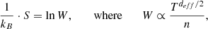
It is finally worth mentioning that the polytropic jump, assuming an adiabatic plasma flow (i.e.,  ), is exactly opposite of the coherent and incoherent events with an absolute value at 0.13. Following Dayeh & Livadiotis (2022), we connected the derived polytropic indices for the two PDS event categories with the entropy gradient and the turbulent heating gradient (Livadiotis et al. 2020) at 1 AU as
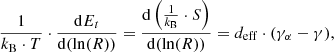
where Et is the turbulent heating of the proton plasma per mass, normalized by the thermal energy, S is the entropy, R is the radial distance, kB is the Boltzmann-Gibbs entropic measure (Livadiotis & McComas 2023), and the adiabatic polytropic index can be written as a function of the effective kinetic degrees of freedom as γα = 1 + 2/deff (see also Appendix A4 for more details). When we assume that deff = 3 and γα = 5/3, even though deff may be affected by the temperature anisotropy (see also Livadiotis & Nicolaou 2021), the entropic gradient jump is three times as strong as the polytropic jump. As shown in Fig. 4, the entropic gradient jump is 0.39 and −0.39 for the coherent and incoherent PDS event protons, respectively. We assumed an adiabatic solar wind with  . This is purely theoretical and valid for slow solar wind streams with an isotropic temperature and three effective degrees of freedom. CMEs, high-speed streams, and stream interaction regions can potentially lead to deviations of the polytropic index from the adiabatic value, which might explain the nonadiabatic polytropic index for the entire Wind dataset shown in Fig. 3. The opposite entropic gradient jump means that the coherent PDS event protons absorb the same amount of energy as the protons that are lost by the incoherent events. This does not necessarily imply a straightforward link between the two categories of PDSs because each PDS event occurs during different time periods. On the other hand, space plasma particle populations act as ensembles of correlated particles, and the related events and phenomena should not be taken simply as isolated, but as an average over a significantly long time period that characterizes the event timescale. Therefore, the aforementioned result, combined with the very similar annual distributions of the coherent and incoherent PDSs (see Fig. B.2), may suggest that their generation mechanisms are somewhat complementary, and the release of energy from the one population is almost entirely consumed by the other population on average and in the long run of these phenomena (note the entropic jumps caused by nearly adiabatic solar wind protons shown in Fig. 4). Nevertheless, we considered only protons in our analysis, and furthermore, we neglected the potential effect of the temperature anisotropy. This feature therefore requires a much more detailed investigation, which is beyond the scope of this paper.
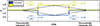 |
Fig. 4. Estimated entropic gradient jumps and |

Acknowledgments
The authors thank the National Space Science Data Center of the Goddard Space Flight Center for the use permission of Wind data and the NASA CDAWeb team for making these data available (http://cdaweb.gsfc.nasa.gov/istp_public/). S.D. was supported by NASA Grant 80NSSC21K0459. The work of C.K., N.V., and L.K. was supported by the Goddard Space Flight Center Heliophysics Internal Scientist Funding Model (ISFM; competitive work package).
References
- Alzate, N., Morgan, H., Viall, N., & Vourlidas, A. 2021, ApJ, 919, 98 [CrossRef] [Google Scholar]
- Antiochos, S. K., Mikić, Z., Titov, V. S., Lionello, R., & Linker, J. A. 2011, ApJ, 731, 112 [Google Scholar]
- Barnes, A. 1966, Phys. Fluids, 9, 1483 [NASA ADS] [CrossRef] [Google Scholar]
- Bowen, T. A., Badman, S., Hellinger, P., & Bale, S. D. 2018, ApJ, 854, L33 [NASA ADS] [CrossRef] [Google Scholar]
- Chandrasekhar, S. 1957, An Introduction to the Study of Stellar Structure, Astrophysical monographs (Dover Publications) [Google Scholar]
- Dayeh, M. A., & Livadiotis, G. 2022, ApJ, 941, L26 [NASA ADS] [CrossRef] [Google Scholar]
- DeForest, C. E., Matthaeus, W. H., Viall, N. M., & Cranmer, S. R. 2016, ApJ, 828, 66 [Google Scholar]
- DeForest, C. E., Howard, R. A., Velli, M., Viall, N., & Vourlidas, A. 2018, ApJ, 862, 18 [Google Scholar]
- Di Matteo, S., Viall, N. M., Kepko, L., et al. 2019, J. Geophys. Res., 124, 837 [NASA ADS] [CrossRef] [Google Scholar]
- Di Matteo, S., Viall, N., & Kepko, L. 2020, https://doi.org/10.5281/zenodo.3703168 [Google Scholar]
- Di Matteo, S., Viall, N. M., & Kepko, L. 2021, J. Geophys. Res., 126 [Google Scholar]
- Di Matteo, S., Villante, U., Viall, N., Kepko, L., & Wallace, S. 2022, J. Geophys. Res., 127, 3 [Google Scholar]
- Di Matteo, S., Katsavrias, C., Kepko, L., & Viall, N. M. 2024, ApJ, submitted [Google Scholar]
- Dialynas, K., Roussos, E., Regoli, L., et al. 2018, J. Geophys. Res.: Space Phys., 123, 8066 [NASA ADS] [CrossRef] [Google Scholar]
- Endeve, E., Holzer, T. E., & Leer, E. 2004, ApJ, 603, 307 [NASA ADS] [CrossRef] [Google Scholar]
- Endeve, E., Lie-Svendsen, O., Hansteen, V. H., & Leer, E. 2005, ApJ, 624, 402 [NASA ADS] [CrossRef] [Google Scholar]
- Gershkovich, I., Lepri, S. T., Viall, N. M., Di Matteo, S., & Kepko, L. 2022, ApJ, 933, 198 [NASA ADS] [CrossRef] [Google Scholar]
- Gershkovich, I., Lepri, S., Viall, N., Di Matteo, S., & Kepko, L. 2023, Sol. Phys., 298, 89 [NASA ADS] [CrossRef] [Google Scholar]
- Grinsted, A., Moore, J. C., & Jevrejeva, S. 2004, Nonlinear Processes Geophys., 11, 561 [NASA ADS] [CrossRef] [Google Scholar]
- Higginson, A. K., & Lynch, B. J. 2018, ApJ, 859, 6 [Google Scholar]
- Hollweg, J. V., Verscharen, D., & Chandran, B. D. G. 2014, ApJ, 788, 35 [NASA ADS] [CrossRef] [Google Scholar]
- Kartalev, M., Dryer, M., Grigorov, K., & Stoimenova, E. 2006, J. Geophys. Res.: Space Phys., 111, A10 [CrossRef] [Google Scholar]
- Kasper, J. C., Lazarus, A. J., Steinberg, J. T., Ogilvie, K. W., & Szabo, A. 2006, J. Geophys. Res., 111 [Google Scholar]
- Katsavrias, C., Preka-Papadema, P., & Moussas, X. 2012, Sol. Phys., 280, 623 [CrossRef] [Google Scholar]
- Katsavrias, C., Hillaris, A., & Preka-Papadema, P. 2016, Adv. Space Res., 57, 2234 [CrossRef] [Google Scholar]
- Katsavrias, C., Papadimitriou, C., Aminalragia-Giamini, S., et al. 2021a, Ann. Geophys., 39, 413 [CrossRef] [Google Scholar]
- Katsavrias, C., Raptis, S., Daglis, I. A., et al. 2021b, Geophys. Res. Lett., 48, 15 [CrossRef] [Google Scholar]
- Katsavrias, C., Papadimitriou, C., Hillaris, A., & Balasis, G. 2022, Atmosphere, 13, 499 [NASA ADS] [CrossRef] [Google Scholar]
- Kepko, L., & Viall, N. M. 2019, J. Geophys. Res. (Space Phys.), 124, 7722 [NASA ADS] [CrossRef] [Google Scholar]
- Kepko, L., Viall, N. M., Antiochos, S. K., et al. 2016, Geophys. Res. Lett., 43, 4089 [NASA ADS] [CrossRef] [Google Scholar]
- Kepko, L., Viall, N. M., & Wolfinger, K. 2020, J. Geophys. Res., 125, e28037 [NASA ADS] [CrossRef] [Google Scholar]
- Kepko, L., Viall, N. M., & DiMatteo, S. 2024, J. Geophys. Res. (Space Phys.), 129, e2023JA031403 [NASA ADS] [CrossRef] [Google Scholar]
- Lavraud, B., Fargette, N., Réville, V., et al. 2020, ApJ, 894, L19 [Google Scholar]
- Lepping, R. P., Acũna, M. H., Burlaga, L. F., et al. 1995, Space. Sci. Rev., 71, 207 [NASA ADS] [CrossRef] [Google Scholar]
- Livadiotis, G. 2016, ApJS, 223, 13 [NASA ADS] [CrossRef] [Google Scholar]
- Livadiotis, G. 2018, Entropy, 20, 799 [NASA ADS] [CrossRef] [Google Scholar]
- Livadiotis, G. 2019, Stats, 2, 416 [CrossRef] [Google Scholar]
- Livadiotis, G., & McComas, D. J. 2011, ApJ, 741, 88 [NASA ADS] [CrossRef] [Google Scholar]
- Livadiotis, G., & McComas, D. J. 2023, Sci. Rep., 13 [CrossRef] [Google Scholar]
- Livadiotis, G., & Nicolaou, G. 2021, ApJ, 909, 127 [NASA ADS] [CrossRef] [Google Scholar]
- Livadiotis, G. P., Dayeh, M. A., & Zank, G. 2020, ApJ, 905, 137 [NASA ADS] [CrossRef] [Google Scholar]
- Lynch, B. J., Edmondson, J. K., & Li, Y. 2014, Sol. Phys., 289, 3043 [Google Scholar]
- Lynch, B. J., Masson, S., Li, Y., et al. 2016, J. Geophys. Res.: Space Phys., 121, 11 [NASA ADS] [CrossRef] [Google Scholar]
- Morlet, J., Arens, G., Fourgeau, E., & Giard, D. 1982, Geophysics, 47, 222 [NASA ADS] [CrossRef] [Google Scholar]
- Nicolaou, G., & Livadiotis, G. 2019, ApJ, 884, 52 [NASA ADS] [CrossRef] [Google Scholar]
- Nicolaou, G., Livadiotis, G., & Moussas, X. 2014, Sol. Phys., 289, 1371 [NASA ADS] [CrossRef] [Google Scholar]
- Nicolaou, G., Livadiotis, G., & Wicks, R. T. 2019, Entropy, 21, 997 [NASA ADS] [CrossRef] [Google Scholar]
- Ogilvie, K. W., Chornay, D. J., Fritzenreiter, R. J., et al. 1995, Space. Sci. Rev., 71, 55 [CrossRef] [Google Scholar]
- Parker, E. 1963, Interplanetary Dynamical Processes, Interscience Monographs and Texts in Physics and Astronomy (Interscience Publishers) [Google Scholar]
- Peterson, E. E., Endrizzi, D. A., Clark, M., et al. 2021, J. Plasma Phys., 87, 4 [CrossRef] [Google Scholar]
- Poirier, N., Réville, V., Rouillard, A. P., Kouloumvakos, A., & Valette, E. 2023, A&A, 677, A108 [NASA ADS] [CrossRef] [EDP Sciences] [Google Scholar]
- Réville, V., Velli, M., Rouillard, A. P., et al. 2020, ApJ, 895, L20 [Google Scholar]
- Siegel, A. F. 1982, Biometrika, 69, 242 [NASA ADS] [CrossRef] [Google Scholar]
- Slepian, D. 1978, Bell Syst. Tech. J., 57, 1371 [NASA ADS] [CrossRef] [Google Scholar]
- Thomson, D. 1982, Proc. IEEE, 70, 1055 [NASA ADS] [CrossRef] [Google Scholar]
- Torrence, C., & Compo, G. P. 1998, Bull. Am. Meteorol. Soc., 79, 61 [Google Scholar]
- Ventura, R., Antonucci, E., Downs, C., et al. 2023, A&A, 675, A170 [NASA ADS] [CrossRef] [EDP Sciences] [Google Scholar]
- Verma, M. K., Roberts, D. A., & Goldstein, M. L. 1995, J. Geophys. Res.: Space Phys., 100, 19839 [NASA ADS] [CrossRef] [Google Scholar]
- Verscharen, D., Klein, K. G., & Maruca, B. A. 2019, Liv. Rev. Sol. Phys., 16, 5 [Google Scholar]
- Viall, N. M., & Vourlidas, A. 2015, ApJ, 807, 176 [Google Scholar]
- Viall, N. M., Kepko, L., & Spence, H. E. 2008, J. Geophys. Res., 113, A7 [Google Scholar]
- Viall, N. M., Kepko, L., & Spence, H. E. 2009a, J. Geophys. Res., 114, A1 [Google Scholar]
- Viall, N. M., Spence, H. E., & Kasper, J. 2009b, Geophys. Res. Lett., 36, L23102 [NASA ADS] [CrossRef] [Google Scholar]
- Viall, N. M., Spence, H. E., Vourlidas, A., & Howard, R. 2010, Sol. Phys., 267, 175 [Google Scholar]
- Viall, N. M., DeForest, C. E., & Kepko, L. 2021, Front. Astron. Space Sci., 8 [Google Scholar]
Appendix A: Methods
A.1. Multitaper method
We estimated the adaptive MTM power spectral density over linearly detrended six-hour intervals using a time half-band width product NW = 2.5 and number of tapers K = 4 (Slepian 1978). This choice of parameters resulted in a Rayleigh frequency of fRay = 1/(NΔt)≈0.05 mHz, where NW = 221 is the number of data points used for the spectral analysis for the Wind spacecraft. Additionally, following Di Matteo et al. (2021), the reliable frequency range corresponds to [2NWfRay, fNy − 2NWfRay]≈0.23–4.87 mHz, in which the upper limit is set by the Nyquist frequency from the Wind spacecraft (fNy = 1/(2Δt)≈5.1 mHz). The power spectral density was then normalized by the best background spectrum representation between those estimated via a maximum likelihood fitting method of a bending power-law model over the original spectrum and its logarithmically binned version (raw+BPL and bin+BPL; see details in Di Matteo et al. 2021).
A.2. Continuous wavelet transform
The analysis of a function in time, F(t), into an orthonormal basis of wavelets is conceptually similar to the MTM. However, the latter is only localized in frequency, while the continuous wavelet transform (henceforward CWT), which is localized in frequency and time, allows for the local decomposition of nonstationary time series, providing a compact, two-dimensional representation. As most astrophysical time series are usually composed of sinusoidal-like oscillations, the most common mother wavelet used is the Morlet wavelet (Morlet et al. 1982), which consists of a complex plane wave modulated by a Gaussian. The equations are
where ω0 is the dimensionless frequency, usually set to 6 to satisfy the admissibility condition, and η is the dimensionless time (see also Katsavrias et al. 2022, for further details).
A.3. Cross-wavelet transform and wavelet coherence
The XWT between two time series X and Y is defined as  , where
  and
and  are the corresponding wavelet spectra (see also Katsavrias et al. 2021a,b). The XWT examines the relation in the time-frequency space between two time series and identifies regions of high common power, while the phase spectrum, obtained from
  , of the XWT represents the relative phase difference between the time series to be compared (Torrence & Compo 1998; Grinsted et al. 2004),
![$$ \begin{aligned} {{\tan ^{ - 1}}\left[\frac{{{\mathop { Im}\nolimits } (\left| {W_n^{XY}(s)} \right|)}}{{{\mathop { Re}\nolimits } (\left| {W_n^{XY}(s)} \right|)}}\right]} . \end{aligned} $$](/articles/aa/full_html/2024/06/aa50217-24/aa50217-24-eq32.gif)
The WTC closely resembles a localized correlation coefficient in time-frequency space (equation A.4) and varies between 0 and 1, corresponding to incoherent and coherent periodic behavior, respectively (Katsavrias et al. 2016, 2022).
Following Grinsted et al. (2004), we defined the wavelet coherence of two time series, X and Y, as
where S is a smoothing operator, and  .
.
The statistical significance level of the WTC was estimated using Monte Carlo methods. Specifically, we generated a large ensemble of first-order autoregressive surrogate dataset pairs with the model coefficient estimated from the input datasets (see also Grinsted et al. 2004). For each synthetic time-series pair, we calculated the WTC values and obtained a distribution from which we defined a significance level for each frequency.
A.4. Connection of the polytropic index with the entropy gradient
Following Livadiotis (2019) and Livadiotis & Nicolaou (2021), we expressed the proton entropy in terms of proton density and temperature as
where S is the entropy, deff are the effective degrees of freedom, n is the number density, and kB is the Boltzmann-Gibbs entropic measure (Livadiotis & McComas 2023).
Furthermore, the density drop can be approximated as

while the polytropic relation for isotropic temperature is

Combining equations A.5, A.6, and A.7, we obtain
where γα = 1 + 2/deff, so that deff = 3 and γα = 5/3.
Combining these equations, we express the entropy gradient as
On the other hand, the gradient of the turbulent heating Et of the proton plasma (per mass), normalized by the thermal energy, is also equal to the deviation of the polytropic index from its adiabatic value (Verma et al. 1995; Livadiotis 2019),
Appendix B: Supplementary figures
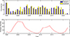 |
Fig. B.2. Annual occurrence of PDS events compared with the annual sunspot number. Top panel: Annual occurrence of coherent and incoherent PDS events depicted with blue and yellow bars, respectively. Bottom panel: Annual sunspot number. |
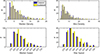 |
Fig. B.3. Distribution of PDS events with respect to the median and maximum proton density (top panels) and the median and maximum proton velocity (bottom panels). Coherent and incoherent PDS events are depicted with blue and yellow bars, respectively. |
All Figures
|
Fig. 1. Example of a coherent (left panels) and incoherent (right panels) event. From top to bottom: time series of np and nα/np (black and blue lines, respectively), wavelet spectrum for np, wavelet power spectrum for nα/np, cross-wavelet spectrum, and wavelet coherence. The vertical dashed red lines correspond to the times at whic the wavelet power, at the corresponding PDS frequency exceeds the 75th quantile of the power of the entire six-hour interval. The solid black lines in all spectra depict the cone of influence, where edge effects in the processing become important. The arrows in XWT and WTC point to the phase relation of the two data series in time-frequency space: (1) Arrows pointing to the right indicate in-phase behavior, and (2) arrows pointing to the left indicate antiphase behavior. |
| In the text | |
|
Fig. 2. Example of a valid derivation of γ satisfying all the criteria set for this study. The left and middle panels show the cross plots of ln(Tp) vs. ln(np) and ln(np) vs. ln(Tp), respectively, with the Wind data shown as black circles (and the corresponding standard deviation with error bars) and the regressed values as the solid red line. The right panel shows Bernoulli’s integral estimate for the same window (black circles) along with the 2% limit (dashed red lines). |
| In the text | |
|
Fig. 3. Distributions of γ for (left panel) the entire Wind dataset spanning 1995–2022, (middle panel) the 341 incoherent PDS events, and (right panel) the 330 coherent PDS events. The solid red lines correspond to the best-fit κ-Gaussian distribution using a weighted nonlinear fit. |
| In the text | |
|
Fig. 4. Estimated entropic gradient jumps and |
| In the text | |
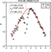 |
Fig. B.1. Same as Figure 3, but for the low-coherence events |
| In the text | |
|
Fig. B.2. Annual occurrence of PDS events compared with the annual sunspot number. Top panel: Annual occurrence of coherent and incoherent PDS events depicted with blue and yellow bars, respectively. Bottom panel: Annual sunspot number. |
| In the text | |
|
Fig. B.3. Distribution of PDS events with respect to the median and maximum proton density (top panels) and the median and maximum proton velocity (bottom panels). Coherent and incoherent PDS events are depicted with blue and yellow bars, respectively. |
| In the text | |
Current usage metrics show cumulative count of Article Views (full-text article views including HTML views, PDF and ePub downloads, according to the available data) and Abstracts Views on Vision4Press platform.
Data correspond to usage on the plateform after 2015. The current usage metrics is available 48-96 hours after online publication and is updated daily on week days.
Initial download of the metrics may take a while.