| Issue |
A&A
Volume 696, April 2025
|
|
|---|---|---|
| Article Number | L20 | |
| Number of page(s) | 8 | |
| Section | Letters to the Editor | |
| DOI | https://doi.org/10.1051/0004-6361/202554483 | |
| Published online | 28 April 2025 | |
Letter to the Editor
The dependence of periodic density structures’ amplitude and length scale on solar wind density within stream interaction regions
1
NASA-Goddard Space Flight Center, Greenbelt, MD, USA
2
Department of Physics, National and Kapodistrian University of Athens, Athens, Greece
3
Physics Department, The Catholic University of America, Washington, DC, USA
⋆ Corresponding author: This email address is being protected from spambots. You need JavaScript enabled to view it.
Received:
11
March
2025
Accepted:
14
April
2025
Abstract
Context. Periodic density structures (PDSs) are a type of solar wind mesoscale structure characterised by quasi-periodic variations in the density of the solar wind ranging from a few minutes to a few hours. They are trains of advected density structures with radial length scales of LR ≈ 100 − 10 000 Mm. Analysis of case studies shows that PDSs can be compressed when embedded in a stream interaction region (SIR), leading to larger density variations and an increased impact on the magnetospheric and radiation belt dynamics.
Aims. We perform an extensive statistical study to identify PDSs embedded in SIRs as well as their corresponding frequency and radial length scale distributions.
Methods. We used an extensive list of 186 SIRs and 1217 embedded PDS events from the entire Wind dataset (1995−2022), spanning more than two solar cycles, to investigate the frequency and radial length scales of PDSs. With the use of wavelet methods, we classified these PDSs as coherent or incoherent, based on the shared periodic behaviour between proton density and the alpha-to-proton ratio, and we derived the corresponding occurrence distributions.
Results. We found that 130 out of 186 SIR events have embedded coherent PDSs, which exhibit an increasing probability of occurrence with increasing frequency (up to ≈3 mHz). Furthermore, the investigation of radial length scales of coherent PDSs in SIRs reveals significant compression compared to PDSs in the ambient solar wind, as the most probable LR values are 120−130 Mm and 160−190 Mm for the slow and fast compressed solar wind, respectively. The coherent PDS LR decreases with a rate of −0.74, while the corresponding amplitude increases with a rate of 0.74 with increasing solar wind proton density, both following a power law function.
Conclusions. Our results indicate that coherent PDSs occur more often than not in SIRs. This is consistent with a picture in which PDSs are formed at the Sun, advected by the solar wind, and enhanced by their interaction with SIRs, while both their radial length scale and amplitude are controlled by the level of compression in the interaction region.
Key words: methods: data analysis / methods: statistical / Sun: corona / Sun: heliosphere / solar wind
© The Authors 2025
 Open Access article, published by EDP Sciences, under the terms of the Creative Commons Attribution License (https://creativecommons.org/licenses/by/4.0), which permits unrestricted use, distribution, and reproduction in any medium, provided the original work is properly cited.
This article is published in open access under the Subscribe to Open model. This email address is being protected from spambots. You need JavaScript enabled to view it. to support open access publication.
1. Introduction
Periodic density structures (PDSs) are a subset of mesoscale structures and a particular constituent of the ambient solar wind (Kepko et al. 2020). These structures have been routinely detected in remote sensing observations of the Sun (Viall & Vourlidas 2015; Poirier et al. 2023; Ventura et al. 2023; Alzate et al. 2024) and in situ observations from the inner heliosphere to 1.0 AU (Kepko et al. 2016; Di Matteo et al. 2019; Gershkovich et al. 2022, 2023; Berriot et al. 2024). Even though their frequencies, which span the 0.1 to 5 mHz range, overlap with Alfvénic fluctuations, PDSs are not waves; rather, they represent periodic spatial intervals of enhanced proton density that are entrained in the solar wind flow (Viall et al. 2008; Kepko et al. 2024). Their radial length scales (LR) at 1 AU vary between a few tens and several thousand Megameteres, while their azimuthal size scales have been estimated as ≈2000 Mm and ≈1000 Mm for PDSs with frequencies less and higher than 1 mHz, respectively (Sanchez-Diaz et al. 2017; Di Matteo et al. 2024). Similar results for the radial sizes have also been inferred from white light images from SOHO and STEREO coronographs (López-Portela et al. 2018; Lyu et al. 2024).
Even though the precise generation mechanisms of PDSs are still debated, several studies using remote-sensing observations of the Sun support the conclusion that they are of solar origin (Viall & Vourlidas 2015; Ventura et al. 2023; Alzate et al. 2024). Furthermore, in situ observations, from 0.3 to 1.0 AU (Kepko et al. 2016; Di Matteo et al. 2019; Kepko et al. 2024), have provided evidence for solar origin theories involving magnetic reconnection and interchange reconnection in the solar corona (e.g., Antiochos et al. 2011; Higginson & Lynch 2018; Réville et al. 2020). In particular, in situ measurements show PDSs associated with small flux ropes (Di Matteo et al. 2019; Lavraud et al. 2020; Katsavrias et al. 2024) and elemental composition; that is, the charge-state ratios or relative abundances of different elements, which are frozen in to the solar wind flow and which do not evolve during their propagation (Viall et al. 2009a; Gershkovich et al. 2022, 2023; Kepko et al. 2024).
The PDSs can impact global magnetospheric (Borovsky & Denton 2006) and radiation belt dynamics through pressure enhancements in the solar wind (Viall et al. 2009b; Di Matteo et al. 2022; Kurien et al. 2024). Therefore, it is highly important to understand their origin and occurrence rate. Recent work has further shown that PDSs are observed within stream interaction regions (SIRs), which are also important drivers of the magnetospheric activity (Kepko & Viall 2019). Furthermore, SIRs drive the variability of the outer radiation belt electrons (Miyoshi & Kataoka 2005; Horne et al. 2018) in a complex way. The high-speed streams (HSSs) that follow the SIRs have been shown to be responsible for enhancements of multi-Megaelectron volt electron fluxes (Katsavrias et al. 2019; Nasi et al. 2022). On the other hand, the compression regions are also a source of broadband magnetospheric ultra-low-frequency (ULF) wave power derived from solar wind dynamic pressure fluctuations, and can lead to substantial loss of energetic particles via indirect magnetopause shadowing induced by the enhanced outward diffusion (Kilpua et al. 2015; Turner et al. 2019). The recent work by Kepko & Viall (2019), studied six SIR events that had embedded PDSs. The authors showed that the structures were amplified and compressed by the SIRs, leading to a series of PDSs with periods typically near 20 min.
In this work, we carry out – for the first time, to our knowledge – an extensive statistical study to identify PDSs embedded in SIRs. To that end, we use a list of 186 SIRs spanning more than two solar cycles. The manuscript is organized as follows. Section 2 describes the data as well as the particular technique we used to identify and classify PDSs. In Section 3, we present the results of the PDS frequency and radial length scale distributions. Finally, we discuss our results and summarize our conclusions in Section 4.
2. Data and event lists
We used solar wind measurements from the Solar Wind Experiment instrument (SWE; Ogilvie et al. 1995) on board the Wind spacecraft near L1, spanning the 1995−2022 time period. The resolution of the SWE data is ≈98 s (the resolution varied over the course of the mission). We considered the solar wind proton (np) and alpha (nα) number density, as well as their ratio (nα/np) obtained using the bi-Maxwellian approach of Kasper et al. (2006).
2.1. Identification of stream interaction regions in Wind data
For the identification of SIR events we used, as a starting point, the list by Grandin et al. (2019), which spans the 1995–2017 time period. We excluded all events that had embedded CMEs and kept only single and isolated events without preconditioning, requiring the average solar wind speed and number density to be less than 400 km/s and 15 cm−3, respectively, for at least 12 h before the start of the event. We further extended the list up to 2022, via visual inspection of solar wind plasma parameters’ time series, with events that also satisfied the aforementioned criteria. The final SIR list includes 186 events (Katsavrias 2025). For each event, we have visually identified the start and end time of the interaction region as the time period when the density increases above 10 particles/cm−3, accompanied by an increase in the IMF magnitude and the proton density gradient (dnp/dt). Similarly, the HSS start time is identified as the time when the solar wind speed exceeds 450 km/s, while the HSS end time corresponds to the first time the solar wind speed drops below 400 km/s after reaching its maximum value. Figure B.1 in the appendix shows an example of an SIR event in our list. We note that we further split the SIR interval into the slow (VSW < 450 km/s) and fast (VSW > 450 km/s) compressed solar wind parts of the SIR (hereafter SCSW and FCSW, respectively), which are denoted in Figure B.1 by the vertical dashed red and green lines, respectively.
2.2. Identification of periodic density structures embedded in SIR events
To identify PDSs in the Wind np time series, we followed a spectral analysis procedure based on the multi-taper method (MTM; Thomson 1982; Di Matteo et al. 2021). First, we estimated the adaptive MTM power spectral density. This was computed over running linearly de-trended six-hour intervals with a 5-minute sliding window. Then, we identified periodic variations in the time series at frequency values at which both the normalized spectrum and an additional statistical test for phase coherence (harmonic F-test) exceed the corresponding 90% confidence threshold. The combination of the MTM and the harmonic F-test is a robust approach that has been extensively tested and employed to identify PDSs in in situ measurements (Viall et al. 2008, 2009a,b; Di Matteo et al. 2019; Kepko et al. 2020, 2024) and remote-sensing observations (Viall et al. 2010; Viall & Vourlidas 2015). Here, we have used the more recent version of this approach (SPD_MTM; Di Matteo et al. 2020, see also Appendix A.1), which was employed in earlier investigations of PDSs in solar wind plasma, composition, and remote sensing measurements (Di Matteo et al. 2022; Gershkovich et al. 2022, 2023; Alzate et al. 2024). Based on this analysis, we identified 2049 PDS events with frequencies in the range of 0.2 to 3.2 mHz. Based on this analysis, we identified 2049 PDS events with frequencies in the range of 0.2 to 3.2 mHz.
2.3. Classification of the identified periodic density structure events
2.3.1. Duration of the periodic density structure events
In order to determine the exact duration of each PDS event, we used the continuous wavelet transform (CWT; Torrence & Compo 1998) and the Morlet wavelet (Morlet et al. 1982) as a mother wavelet (see details in Appendix A.2), following Katsavrias et al. (2012). We calculated the wavelet power spectral density of the proton density time series in each of the 2049 six-hour intervals identified as containing a PDS via the MTM method. Then, we isolated the time periods in which the wavelet power at the corresponding PDS frequency exceeded the 75th percentile of the wavelet power during the six-hour interval (again at the same frequency as the one identified with the MTM method). Finally, in order to avoid any dubious detections, we required the duration of each PDS to be at least twice its period. This criterion produced a list of 858 and 359 PDS events during the SCSW and FCSW, respectively.
2.3.2. Classification of periodic density structure events in terms of solar corona origin
Next, we used the cross-wavelet transform and the wavelet coherence (henceforward, XWT and WTC, respectively) between the np and nα/np time series, following Katsavrias et al. (2024) (see also Appendix A.3 for more details).
We classified each of the 1217 PDS events into three categories as follows:
-
In coherent events, the XWT power between np and nα/np exceeds the 75th percentile of the XWT power in the six-hour interval at the corresponding frequency, and at the same time the corresponding WTC median is higher than 0.7.
-
In low-coherence events, the XWT power between np and nα/np exceeds the 75th percentile of the XWT power in the six-hour interval at the corresponding frequency, but the corresponding WTC median is lower than 0.7.
-
In incoherent events, the XWT power between np and nα/np is lower than the 75th quantile of the XWT power in the six-hour interval at the corresponding frequency.
Table 1 summarizes the results of the classification process. We note that the events classified as low-coherence may include events that indeed exhibit oscillations at the same frequency between np and nα/np, as a result of a common physical mechanism, but that simply did not pass our threshold (i.e. 0.7). Consequently, in order to avoid any confusion, we do not include the low-coherence events in the following discussion.
Number of PDS events in each category.
3. Results
3.1. Distribution of PDS frequencies
Figure 1 shows the PDS frequency distributions in the 0.2−3.2 mHz range binned in groups with Δf = 0.3 mHz, which is the spectral window bandwidth. As is shown in the left panel, the PDS frequency distribution during the 186 SIR events exhibits an increasing probability with increasing frequency as well as two local maxima at the 1.7−2.3 and at the 2.6−3.2 mHz frequency range. These maxima are in agreement with Di Matteo et al. (2024), who studied slow solar wind intervals with PDSs observed by the Wind and ARTEMIS-P1 spacecraft. They found local enhancements centred at ≈1.9 mHz and with more variability within ≈2.7−2.9 mHz and the ≈3.2−3.8 mHz frequency range (see also Figure 5 in Di Matteo et al. 2024). Nevertheless, their PDS distributions, in contrast to this study, manifest the highest occurrence of events at ≈0.5−0.8 mHz and then a decreasing decreasing occurrence rate. We note that the negligible number of PDS events with frequencies less than 0.5 mHz is due to the 6-hour window used in this study. In detail, a significant fraction of the power corresponding to frequencies less than 0.5 mHz is inside the cone of influence of the wavelet spectrum (see also Figure B.2 in the appendix), and thus the valid duration of the corresponding PDS is usually less than two times its period. Therefore, such events are filtered out by our PDS detection criterion (Section 2.3.1).
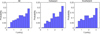 |
Fig. 1. Distribution of 1217 PDS frequencies during the 186 SIRs for PDSs with a duration of at least twice the corresponding PDS period. From left to right: the frequency distribution of all PDSs, the frequency distribution of the coherent PDSs, and the frequency distribution of the incoherent PDSs, respectively. |
Next, we examined the frequency distribution for coherent and incoherent events, separately. The reasoning behind this separation lies in the theories about their generation mechanisms. Coherent events – ones that share periodic behaviour in both proton density and nα/np – are accompanied by strong evidence of a coronal origin and by processes involving magnetic reconnection at the solar corona and the periodic release of small flux ropes (Higginson & Lynch 2018; Réville et al. 2020; Katsavrias et al. 2024). On the other hand, incoherent events can be associated with different generation mechanisms either at the Sun – interchange reconnection processes (DeForest et al. 2016; Viall et al. 2021) – or, in the expanding solar wind, parametric instability, in which an Alfvén wave decays into a daughter Alfvén wave and an MHD slow mode, which compresses the plasma and yields density fluctuations (Hollweg et al. 2014; Bowen et al. 2018).
Coherent PDS events (middle panel of Figure 1) exhibit a very similar frequency distribution as the probability increases with increasing frequency and local maxima exist at ≈2 and ≈3 mHz. These maxima are in agreement with what has been found in 25 years data of ambient solar wind by Kepko et al. (2024). The latter authors found a broad occurrence enhancement in both the proton and nα/np distributions between 1 and 3 mHz, with local maxima at ≈2.1, 2.5 and 2.9 mHz (see also Figure 5 in Kepko et al. 2024).
Finally, incoherent PDS events (right panel of Figure 1) also exhibit local maxima at the same frequency range, yet less pronounced ones than for the coherent PDS events. Furthermore, the distribution seems flatter in the ≈0.5−2.5 mHz range.
3.2. Distribution of coherent PDS radial length scale (LR)
Even though the frequency distribution of PDSs embedded in SIRs exhibit significant differences from the ones in the ambient solar wind, working in the frequency domain does not account for any compression or relaxation of the density structures that may have occurred in transit and may result in different occurrence rate of periodicities in length scale (Viall et al. 2008, 2009b). To that end, we converted the frequencies using the mean solar wind radial velocity as: LR = VR/fPDS, where VR is the mean solar wind radial velocity, in radial-tangential-normal (RTN) co-ordinates, for each PDS event and fPDS the corresponding frequency. Incoherent events were excluded from further analysis in the radial length scale domain since, as was discussed in the previous subsection, they may be either structures or waves formed either in the corona or generated en route, and thus a conversion to radial length scale could be misleading.
Figure 2 shows both the frequency (top panels) and radial length scale (bottom panels) distribution of the coherent PDS events for the entire SIR duration (left panels) as well as the SCSW and FCSW parts (middle and right panels, respectively). As is shown, the frequency distribution of coherent PDS events exhibits small differences from the SCSW to the FCSW part. In contrast, the conversion to LR reveals significant differences between the distributions during the two SIR parts. The LR distribution during the SCSW exhibits a pronounced enhancement of the occurrence rate in the 110−160 Mm range, with a peak at 120−130 Mm and a decreasing trend for LR > 130 Mm. A secondary peak at 200−220 Mm also exists. The LR distribution during the fast compressed solar wind exhibits a completely different behaviour. Small structures, of LR < 130 Mm, are completely absent. A pronounced enhancement of the occurrence rate is exhibited in the 160−190 Mm range, with a peak at 160−170 Mm. Furthermore, there are possibly secondary peaks at 200−210 and 270−280 Mm.
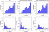 |
Fig. 2. Distribution of the coherent PDS frequencies (top panels) and radial length scales (bottom panels) during the 186 SIR events. From left to right: the distributions during the entire SIR and the distributions during the SCSW and FCSW, respectively. |
The pronounced differences between the LR distributions of SCSW and FCSW may be due to the fact that we are converting a rather similar distribution using lower and higher values of solar wind speed. On the other hand, these differences may reflect the level of compression in the interaction region, since SCSW exhibits higher-density values compared to the fast compressed solar wind. To further test this scenario, we performed a binning of the coherent PDSs LR with respect to solar wind proton density (np). We note that the binning was performed in 25 bins that had variable lengths but contained the same amount of data points. The left panel in Figure 3 shows the dependence of the median LR on the median np in each bin, along with the inter-quartile range. As is shown, there is a decrease in the LR with increasing np, which resembles a power law. Moreover, the non-linear fitting on the data (solid red line) results in a rate of decrease at ≈−0.74. Along the same line, the right panel of Figure 3 shows the dependence of the median amplitude (A), derived from the CWT, on the median np in each bin. The amplitude increases with increasing np and the corresponding power law fitting gives a rate at ≈0.74.
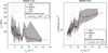 |
Fig. 3. Dependence of the coherent PDS radial length scale (left panel) and power spectral density (right panel) on solar wind proton density. Grey dots correspond to the data and the solid black lines to the median of each np bin, respectively, while the shaded grey area is the inter-quartile range. The power law fit on the data is depicted with the solid red line, while the root mean square error (RMSE) is given at the top of each panel. |
4. Discussion and conclusions
Using more than two solar cycles of Wind measurements (1995–2022), we have identified a list of 186 single and isolated SIRs, without preconditioning, and 1217 PDS events embedded in them. These PDS events are further classified into two categories: (a) coherent events, for which the corresponding frequency was detected in both np and nα/np with high coherence, and (b) incoherent events, for which the corresponding frequency was detected in np alone. This classification allows us to separately examine structures of unambiguous coronal origin and ambiguous events (events that are either of coronal origin without being accompanied by the same elemental abundance or events associated with different generation mechanisms at the Sun or in the expanding solar wind).
Our results show that distributions of PDS within SIRs exhibit an increasing probability with increasing frequency. Moreover, incoherent events exhibit a slightly flatter distribution compared to the coherent events. To further account for any compression or relaxation of the density structures that may have occurred in transit, we have converted the PDS frequencies to their corresponding radial length scales. This has been performed for coherent events only, since the conversion of incoherent events, if they are not structures formed in the corona, could be misleading.
The coherent PDS events exhibit their maximum probability at 120−130 Mm and at 160−190 Mm during the SCSW and FCSW, respectively. These peaks differ from the ones found in the ambient solar wind. As is shown in Figure 5 in Kepko et al. (2024), the LR distributions of PDS events during the slow and fast ambient solar wind exhibit pronounced peaks at ≈180 and ≈250 Mm, respectively (see also Figure B.4) in the appendix for a one-to-one comparison in the case of the slow solar wind). Furthermore, the coherent events have an LR distribution that is highly dependent on proton number density levels – the LR decreases with increasing np at a rate of ≈−0.74 – while their corresponding amplitude increases with increasing np, remarkably at the same rate. The latter provides a rough estimate of the relation between radial length scale and PDS amplitude given as Lr = 75A−1. These results are in very good agreement with Kepko & Viall (2019), who examined six SIR events that contained PDSs. The latter authors present evidence that these periodic structures appear to have been pre-existing structures in the ambient solar wind that were then amplified and compressed at the interaction region between the high and slow speed flow. Here, we present a statistical study using a large sample of both SIRs and the embedded PDS in them that verify the aforementioned results.
Our findings for the coherent PDS events are summarized as follows:
-
The coherent event distribution at the SCSW exhibits a pronounced enhancement of probability in the 110−160 Mm range, with a peak at 120−130 Mm and a decreasing trend for LR > 130 Mm.
-
The corresponding distribution at the FCSW exhibits a pronounced enhancement of the probability in the 160−190 Mm range.
-
The coherent event distribution during both SCSW and FCSW exhibits maxima at lower LR compared to the ones in the ambient solar wind.
-
The coherent PDS LR decreases with a rate of −0.74, while their amplitude increases at the same rate with increasing solar wind proton density, both following a power law function.
Our results are consistent with PDSs formed in the corona and are embedded and compressed within the SIRs. Our findings are important for understanding not only the occurrence rate and propagation of PDSs in the interplanetary medium, but also their impact on the global magnetospheric and radiation belt dynamics. These structures can drive discrete magnetospheric pulsations at the apparent frequency of the advecting PDS structure because of the direct changes to the solar wind dynamic pressure created by the changing proton number density (Viall et al. 2008; Kepko et al. 2002). This impact may be greater for PDSs that are embedded in SIRs, since they are associated with larger-amplitude-density variations that together with increasing speed would result in even larger dynamic pressure variations.
The SIRs are key drivers of the variability in the outer radiation belt electrons as they can lead to both multi-Megaelectron volt electron acceleration and substantial loss (Kilpua et al. 2015; Turner et al. 2019). In a recent work, Katsavrias et al. (2019) studied an SIR driven geospace disturbance that led to significant loss of relativistic electrons from the heart of the outer belt, even though the maximum compression of the magnetopause was at L ≈ 8. The latter authors attribute the losses to the mechanism of indirect magnetopause shadowing; that is, high ULF wave activity, which scatters electrons to larger L-shells where they can be lost more effectively at the outer boundary (Turner et al. 2012; Katsavrias et al. 2015). Nevertheless, similar SIR-driven geospace disturbances do not seem to produce such significant losses (Nasi et al. 2022). Therefore, a question arises concerning the actual mechanism for these induced losses, since not all SIRs have embedded coherent PDSs (130 of the 186 SIR events in our study had embedded coherent PDSs): whether the radiation belt electron losses driven by field line resonances are induced by the pressure pulse itself, or the ULF waves are a direct impact of coherent PDSs embedded in the SIR.
Data availability
The SIR list is publicly available at https://zenodo.org/records/15225254
Acknowledgments
This material is based upon work supported by the National Aeronautics and Space Administration through the completed Heliophysics Internal Scientist Funding Model Program. The authors thank the National Space Science Data Center of the Goddard Space Flight Center for the use permission of Wind data and the NASA CDAWeb team for making these data available (http://cdaweb.gsfc.nasa.gov/istp_public). S.D. was also supported by NASA Grant 80NSSC21K0459.
References
- Alzate, N., Di Matteo, S., Morgan, H., Viall, N., & Vourlidas, A. 2024, ApJ, 973, 130 [Google Scholar]
- Antiochos, S. K., Mikić, Z., Titov, V. S., Lionello, R., & Linker, J. A. 2011, ApJ, 731, 112 [Google Scholar]
- Berriot, E., Démoulin, P., Alexandrova, O., Zaslavsky, A., & Maksimovic, M. 2024, A&A, 686, A114 [NASA ADS] [CrossRef] [EDP Sciences] [Google Scholar]
- Borovsky, J. E., & Denton, M. H. 2006, J. Geophys. Res.: Space Phys., 111, A07S08 [Google Scholar]
- Bowen, T. A., Badman, S., Hellinger, P., & Bale, S. D. 2018, ApJ, 854, L33 [NASA ADS] [CrossRef] [Google Scholar]
- DeForest, C. E., Matthaeus, W. H., Viall, N. M., & Cranmer, S. R. 2016, ApJ, 828, 66 [Google Scholar]
- Di Matteo, S., Viall, N. M., Kepko, L., et al. 2019, J. Geophys. Res., 124, 837 [NASA ADS] [CrossRef] [Google Scholar]
- Di Matteo, S., Viall, N., & Kepko, L. 2020, https://doi.org/10.5281/zenodo.3703168 [Google Scholar]
- Di Matteo, S., Viall, N. M., & Kepko, L. 2021, J. Geophys. Res., 126, e28748 [Google Scholar]
- Di Matteo, S., Villante, U., Viall, N., Kepko, L., & Wallace, S. 2022, J. Geophys. Res., 127, e2021JA030144 [Google Scholar]
- Di Matteo, S., Katsavrias, C., Kepko, L., & Viall, N. M. 2024, ApJ, 969, 67 [Google Scholar]
- Gershkovich, I., Lepri, S. T., Viall, N. M., Di Matteo, S., & Kepko, L. 2022, ApJ, 933, 198 [NASA ADS] [CrossRef] [Google Scholar]
- Gershkovich, I., Lepri, S., Viall, N., Di Matteo, S., & Kepko, L. 2023, Sol. Phys., 298, 89 [NASA ADS] [CrossRef] [Google Scholar]
- Grandin, M., Aikio, A. T., & Kozlovsky, A. 2019, J. Geophys. Res.: Space Phys., 124, 3871 [NASA ADS] [CrossRef] [Google Scholar]
- Grinsted, A., Moore, J. C., & Jevrejeva, S. 2004, Nonlinear Process. Geophys., 11, 561 [CrossRef] [Google Scholar]
- Higginson, A. K., & Lynch, B. J. 2018, ApJ, 859, 6 [Google Scholar]
- Hollweg, J. V., Verscharen, D., & Chandran, B. D. G. 2014, ApJ, 788, 35 [NASA ADS] [CrossRef] [Google Scholar]
- Horne, R. B., Phillips, M. W., Glauert, S. A., et al. 2018, Space Weather, 16, 1202 [CrossRef] [Google Scholar]
- Kasper, J. C., Lazarus, A. J., Steinberg, J. T., Ogilvie, K. W., & Szabo, A. 2006, J. Geophys. Res.: Space Phys., 111, A03105 [Google Scholar]
- Katsavrias, C. 2025, https://doi.org/10.5281/zenodo.15225254 [Google Scholar]
- Katsavrias, C., Preka-Papadema, P., & Moussas, X. 2012, Sol. Phys., 280, 623 [CrossRef] [Google Scholar]
- Katsavrias, C., Daglis, I. A., Turner, D. L., et al. 2015, Geophys. Res. Lett., 42, 10,521 [NASA ADS] [CrossRef] [Google Scholar]
- Katsavrias, C., Hillaris, A., & Preka-Papadema, P. 2016, Adv. Space Res., 57, 2234 [CrossRef] [Google Scholar]
- Katsavrias, C., Sandberg, I., Li, W., et al. 2019, J. Geophys. Res.: Space Phys., 124, 4402 [Google Scholar]
- Katsavrias, C., Papadimitriou, C., Aminalragia-Giamini, S., et al. 2021a, Ann. Geophys., 39, 413 [CrossRef] [Google Scholar]
- Katsavrias, C., Raptis, S., Daglis, I. A., et al. 2021b, Geophys. Res. Lett., 48, e93611 [Google Scholar]
- Katsavrias, C., Papadimitriou, C., Hillaris, A., & Balasis, G. 2022, Atmosphere, 13, 499 [NASA ADS] [CrossRef] [Google Scholar]
- Katsavrias, C., Nicolaou, G., Di Matteo, S., et al. 2024, A&A, 686, L10 [NASA ADS] [CrossRef] [EDP Sciences] [Google Scholar]
- Kepko, L., & Viall, N. M. 2019, J. Geophys. Res.: Space Phys., 124, 7722 [Google Scholar]
- Kepko, L., Spence, H. E., & Singer, H. J. 2002, Geophys. Res. Lett., 29, 39 [Google Scholar]
- Kepko, L., Viall, N. M., Antiochos, S. K., et al. 2016, Geophys. Res. Lett., 43, 4089 [NASA ADS] [CrossRef] [Google Scholar]
- Kepko, L., Viall, N. M., & Wolfinger, K. 2020, J. Geophys. Res., 125, e28037 [NASA ADS] [CrossRef] [Google Scholar]
- Kepko, L., Viall, N. M., & DiMatteo, S. 2024, J. Geophys. Res.: Space Phys., 129, e2023JA031403 [Google Scholar]
- Kilpua, E. K. J., Hietala, H., Turner, D. L., et al. 2015, Geophys. Res. Lett., 42, 3076 [NASA ADS] [CrossRef] [Google Scholar]
- Kurien, L. V., Kanekal, S. G., Di Matteo, S., et al. 2024, J. Geophys. Res.: Space Phys., 129, e2024JA032614 [Google Scholar]
- Lavraud, B., Fargette, N., Réville, V., et al. 2020, ApJ, 894, L19 [Google Scholar]
- López-Portela, C., Panasenco, O., Blanco-Cano, X., & Stenborg, G. 2018, Sol. Phys., 293, 99 [Google Scholar]
- Lyu, S., Wang, Y., Li, X., Zhang, Q., & Liu, J. 2024, ApJ, 962, 170 [Google Scholar]
- Miyoshi, Y., & Kataoka, R. 2005, Geophys. Res. Lett., 32, L21105 [Google Scholar]
- Morlet, J., Arens, G., Fourgeau, E., & Giard, D. 1982, Geophysics, 47, 222 [NASA ADS] [CrossRef] [Google Scholar]
- Nasi, A., Katsavrias, C., Daglis, I. A., et al. 2022, Front. Astron. Space Sci., 9, 949788 [Google Scholar]
- Ogilvie, K. W., Chornay, D. J., Fritzenreiter, R. J., et al. 1995, Space Sci. Rev., 71, 55 [Google Scholar]
- Poirier, N., Réville, V., Rouillard, A. P., Kouloumvakos, A., & Valette, E. 2023, A&A, 677, A108 [NASA ADS] [CrossRef] [EDP Sciences] [Google Scholar]
- Réville, V., Velli, M., Rouillard, A. P., et al. 2020, ApJ, 895, L20 [Google Scholar]
- Sanchez-Diaz, E., Rouillard, A. P., Davies, J. A., et al. 2017, ApJ, 851, 32 [Google Scholar]
- Slepian, D. 1978, Bell Syst. Tech. J., 57, 1371 [NASA ADS] [CrossRef] [Google Scholar]
- Thomson, D. 1982, Proc. IEEE, 70, 1055 [NASA ADS] [CrossRef] [Google Scholar]
- Torrence, C., & Compo, G. P. 1998, Bull. Am. Meteorol. Soc., 79, 61 [Google Scholar]
- Turner, D. L., Shprits, Y., Hartinger, M., & Angelopoulos, V. 2012, Nat. Phys., 8, 208 [Google Scholar]
- Turner, D. L., Kilpua, E. K. J., Hietala, H., et al. 2019, J. Geophys. Res.: Space Phys., 124, 1013 [Google Scholar]
- Ventura, R., Antonucci, E., Downs, C., et al. 2023, A&A, 675, A170 [NASA ADS] [CrossRef] [EDP Sciences] [Google Scholar]
- Viall, N. M., & Vourlidas, A. 2015, ApJ, 807, 176 [Google Scholar]
- Viall, N. M., Kepko, L., & Spence, H. E. 2008, J. Geophys. Res., 113 A07101 [Google Scholar]
- Viall, N. M., Spence, H. E., & Kasper, J. 2009a, Geophys. Res. Lett., 36, L23102 [NASA ADS] [CrossRef] [Google Scholar]
- Viall, N. M., Kepko, L., & Spence, H. E. 2009b, J. Geophys. Res., 114, A01201 [Google Scholar]
- Viall, N. M., Spence, H. E., Vourlidas, A., & Howard, R. 2010, Sol. Phys., 267, 175 [Google Scholar]
- Viall, N. M., DeForest, C. E., & Kepko, L. 2021, Front. Astron. Space Sci., 8, 735034 [Google Scholar]
Appendix A: Methods
A.1. Multitaper method
We estimated the adaptive MTM power spectral density over running linearly detrended six-hour intervals using a time half-band width product NW = 2.5 and number of tapers K = 4 (Slepian 1978). This choice of parameters resulted in a Rayleigh frequency of fRay ≈ 0.05 mHz and a spectral window bandwidth of ≈2NWfRay ≈ 0.3 mHz. The power spectral density was then normalized by the best background spectrum representation between those estimated via a maximum likelihood fitting method of a bending power-law model over the original spectrum and its logarithmically binned version (raw+BPL and bin+BPL; see details in Di Matteo et al. 2021). The background spectrum was estimated in the frequency range between ≈0.2 and ≈3.2 mHz, within the reliable frequency range as defined by Di Matteo et al. (2021). The use of this frequency range allows a good estimate of the spectrum background within SIR (ratio of spectrum versus background close to unity).
A.2. Continuous wavelet transform
The analysis of a function in time, F(t), into an orthonormal basis of wavelets is conceptually similar to the MTM. However, the latter is only localized in frequency, while the continuous wavelet transform (henceforward CWT), which is localized in frequency and time, allows for the local decomposition of nonstationary time series, providing a compact, two-dimensional representation. As most astrophysical time series are usually composed of sinusoidal-like oscillations, the most common mother wavelet used is the Morlet wavelet (Morlet et al. 1982), which consists of a complex plane wave modulated by a Gaussian. The equations are
 (A.1)
(A.1)
 (A.2)
(A.2)
where ω0 is the dimensionless frequency, usually set to 6 to satisfy the admissibility condition, and η is the dimensionless time (see also Katsavrias et al. 2022, for further details).
A.3. Cross-wavelet transform and wavelet coherence
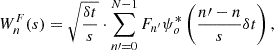
The XWT between two time series X and Y is defined as  , where
  and
and  are the corresponding wavelet spectra (see also Katsavrias et al. 2021a,b). The XWT examines the relation in the time-frequency space between two time series and identifies regions of high common power, while the phase spectrum, obtained from arg(WnXY), of the XWT represents the relative phase difference between the time series to be compared (Torrence & Compo 1998; Grinsted et al. 2004),
![Mathematical equation: $$ \begin{aligned} {{\tan ^{-1}}\left[\frac{{{\mathop {Im}\nolimits } (\left|{W_n^{XY}(s)}\right|)}}{{{\mathop {Re}\nolimits } (\left|{W_n^{XY}(s)}\right|)}}\right]}. \end{aligned} $$](/articles/aa/full_html/2025/04/aa54483-25/aa54483-25-eq6.gif) (A.3)
(A.3)
The WTC closely resembles a localized correlation coefficient in time–frequency space (equation A.4) and varies between 0 and 1, corresponding to incoherent and coherent periodic behavior, respectively (Katsavrias et al. 2016, 2022).
Following Grinsted et al. (2004), we defined the wavelet coherence of two time series, X and Y, as
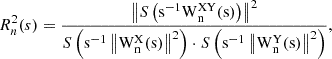 (A.4)
(A.4)
where S is a smoothing operator, and Rn2(s)≤1.
The statistical significance level of the WTC was estimated using Monte Carlo methods. Specifically, we generated a large ensemble of first-order autoregressive surrogate dataset pairs with the model coefficient estimated from the input datasets (see also Grinsted et al. 2004). For each synthetic time-series pair, we calculated the WTC values and obtained a distribution from which we defined a significance level for each frequency.
Appendix B: Supplementary figures
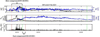 |
Fig. B.1. Example of an SIR event. Top panel: IMF and its z-component (black and blue solid lines, respectively). Middle panel: Proton number density and solar wind bulk speed. Bottom panel: Proton number density gradient. The red and green vertical lines delimit the SIR region and the fast solar wind stream (> 450 km/s), respectively. The brackets further indicate the SCSW (first red to first green vertical line) and FCSW (first green to second red vertical line). |
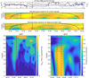 |
Fig. B.2. Example of a coherent event. From top to bottom: Time series of np and nα/np (black and blue lines, respectively), wavelet spectrum for np, wavelet power spectrum for nα/np, cross-wavelet spectrum, and wavelet coherence. The vertical dashed red lines correspond to the times at which the wavelet power, at the corresponding PDS frequency exceeds the 75th quantile of the power of the entire six-hour interval. The solid black lines in all spectra depict the cone of influence, where edge effects in the processing become important. |
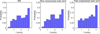 |
Fig. B.3. Distribution of the incoherent PDS frequencies during the 186 SIR events. From left to right: the distributions during the entire SIR and the distributions during the SCSW and FCSW, respectively. |
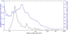 |
Fig. B.4. Comparison of the distribution of the coherent PDS radial length scale during the SCSW with the 25-year occurrence distributions for the slow solar wind found by Kepko et al. (2024). |
All Tables
All Figures
|
Fig. 1. Distribution of 1217 PDS frequencies during the 186 SIRs for PDSs with a duration of at least twice the corresponding PDS period. From left to right: the frequency distribution of all PDSs, the frequency distribution of the coherent PDSs, and the frequency distribution of the incoherent PDSs, respectively. |
| In the text | |
|
Fig. 2. Distribution of the coherent PDS frequencies (top panels) and radial length scales (bottom panels) during the 186 SIR events. From left to right: the distributions during the entire SIR and the distributions during the SCSW and FCSW, respectively. |
| In the text | |
|
Fig. 3. Dependence of the coherent PDS radial length scale (left panel) and power spectral density (right panel) on solar wind proton density. Grey dots correspond to the data and the solid black lines to the median of each np bin, respectively, while the shaded grey area is the inter-quartile range. The power law fit on the data is depicted with the solid red line, while the root mean square error (RMSE) is given at the top of each panel. |
| In the text | |
|
Fig. B.1. Example of an SIR event. Top panel: IMF and its z-component (black and blue solid lines, respectively). Middle panel: Proton number density and solar wind bulk speed. Bottom panel: Proton number density gradient. The red and green vertical lines delimit the SIR region and the fast solar wind stream (> 450 km/s), respectively. The brackets further indicate the SCSW (first red to first green vertical line) and FCSW (first green to second red vertical line). |
| In the text | |
|
Fig. B.2. Example of a coherent event. From top to bottom: Time series of np and nα/np (black and blue lines, respectively), wavelet spectrum for np, wavelet power spectrum for nα/np, cross-wavelet spectrum, and wavelet coherence. The vertical dashed red lines correspond to the times at which the wavelet power, at the corresponding PDS frequency exceeds the 75th quantile of the power of the entire six-hour interval. The solid black lines in all spectra depict the cone of influence, where edge effects in the processing become important. |
| In the text | |
|
Fig. B.3. Distribution of the incoherent PDS frequencies during the 186 SIR events. From left to right: the distributions during the entire SIR and the distributions during the SCSW and FCSW, respectively. |
| In the text | |
|
Fig. B.4. Comparison of the distribution of the coherent PDS radial length scale during the SCSW with the 25-year occurrence distributions for the slow solar wind found by Kepko et al. (2024). |
| In the text | |
Current usage metrics show cumulative count of Article Views (full-text article views including HTML views, PDF and ePub downloads, according to the available data) and Abstracts Views on Vision4Press platform.
Data correspond to usage on the plateform after 2015. The current usage metrics is available 48-96 hours after online publication and is updated daily on week days.
Initial download of the metrics may take a while.