| Issue |
A&A
Volume 669, January 2023
|
|
|---|---|---|
| Article Number | A153 | |
| Number of page(s) | 14 | |
| Section | The Sun and the Heliosphere | |
| DOI | https://doi.org/10.1051/0004-6361/202243603 | |
| Published online | 26 January 2023 | |
Characterizing the specific energy and pressure in near-Earth magnetic clouds
1
Indian Institute of Science Education and Research, Pune Dr. Homi Bhabha Road, Pashan, Pune 411008, India
e-mail: This email address is being protected from spambots. You need JavaScript enabled to view it.
2
The Johns Hopkins University Applied Physics Laboratory, Laurel, MD 20723, USA
3
Heliophysics Science Division, NASA-Goddard Space Flight Center, Greenbelt, MD 20771, USA
4
Department of Physics, The University of Arizona, Tucson, AZ 85721, USA
5
Department of Climate and Space Science and Engineering, University of Michigan, Ann Arbor, MI 48109, USA
Received:
22
March
2022
Accepted:
29
October
2022
Abstract
Context. The pressure and energy density of the gas and magnetic field inside solar coronal mass ejections (in relation to that in the ambient solar wind) is thought to play an important role in determining their dynamics as they propagate through the heliosphere.
Aims. We compare the specific energy (erg g−1), comprising kinetic (Hk), thermal (Hth) and magnetic field (Hmag) contributions, inside magnetic clouds (MCs) and the solar wind background. We examine whether the excess thermal+magnetic pressure and specific energy inside MCs (relative to the background) are correlated with their propagation and internal expansion speeds. We consider whether the excess thermal+magnetic specific energy inside MCs might cause them to resemble rigid bodies in the context of aerodynamic drag.
Methods. We used near-Earth in situ data from the WIND spacecraft to identify a sample of 152 well-observed interplanetary coronal mass ejections and their MC counterparts. We compared various metrics based on these data to address our questions.
Results. We find that the total specific energy (H) inside MCs is approximately equal to that in the background solar wind. We find that the excess (thermal+magnetic) pressure and specific energy are not well correlated with the near-Earth propagation and expansion speeds. We find that the excess thermal+magnetic specific energy is greater or equivalent to the specific kinetic energy of the solar wind incident in 81–89% of the MCs we study. This might explain how MCs retain their structural integrity and resist deformation by the solar wind bulk flow.
Key words: magnetohydrodynamics (MHD) / Sun: coronal mass ejections (CMEs) / methods: data analysis / methods: statistical / solar wind
© The Authors 2023
 Open Access article, published by EDP Sciences, under the terms of the Creative Commons Attribution License (https://creativecommons.org/licenses/by/4.0), which permits unrestricted use, distribution, and reproduction in any medium, provided the original work is properly cited.
This article is published in open access under the Subscribe-to-Open model. This email address is being protected from spambots. You need JavaScript enabled to view it. to support open access publication.
1. Introduction
Earth-directed coronal mass ejections (CMEs) originating from the solar corona are the primary drivers of geomagnetic storms. Realistic estimates of Sun-Earth CME propagation times and arrival velocities are therefore an important component of space weather forecasting. Understanding the dynamics of CMEs and the forces leading to their propagation and expansion is crucial to this endeavor. Approaches to this problem include early analytical models for the entire Sun-Earth propagation (Chen 1996; Kumar & Rust 1996) and semi-analytical models that are only applicable to the aerodynamic drag-dominated phase of the propagation (Cargill 2004; Sachdeva et al. 2015; Vršnak et al. 2013) as well as detailed 3D magnetohydrodynamic (MHD) models (Linker et al. 1999; Odstrcil & Pizzo 2009; Keppens et al. 2020; Tóth et al. 2012). A number of efforts have been focused on characterizing the internal magnetic structure of the interplanetary counterparts of CMEs (ICMEs) (Klein & Burlaga 1982; Nieves-Chinchilla et al. 2016), while others have been centered on comprehensive characterizations of ICME properties (Richardson & Cane 2010; Temmer 2021; Forsyth et al. 2006).
Despite these advances, there are still some fairly basic issues that remain to be addressed in this area and CME expansion provides a concrete window into some of these open questions. It is well known that CMEs propagate as well as expand as they travel through the heliosphere, namely, CMEs are observed to expand in typical coronagraph fields of view (St. Cyr et al. 2000) and beyond (Lugaz et al. 2010; Webb et al. 2009). In addition, CME expansion has been confirmed using in situ observations in the heliosphere (Bothmer & Schwenn 1998; Wang & Richardson 2004) and near the Earth (Dasso et al. 2007). The expansion is thought to occur because the interior of the CME is subject to a great amount of pressure with respect to its surroundings (e.g., von Steiger & Richardson 2006; Scolini et al. 2019; Démoulin & Dasso 2009; Verbeke et al. 2022), although some authors have contended that the expansion is an outcome of CME magnetic field rearrangement (Kumar & Rust 1996). Some have (e.g., Gopalswamy et al. 2014, 2015; Kassa Dagnew et al. 2022) considered whether the abundance of halo CMEs during solar cycle 24 is because the ambient solar wind pressure is generally lower, leading CMEs to be more overly pressurized (with respect to their surroundings) than usual. Generally, CME expansion speeds are also known to be lower than the Alfvén speeds in the ambient solar wind (Klein & Burlaga 1982; Lugaz et al. 2020) – this is another observation drawn from comparisons between the CME plasma and that of the surrounding solar wind. Also, CME identification using in situ data relies on a comparison between the CME and the ambient solar wind plasma – and one of the more widely accepted criteria for identifying near-Earth magnetic clouds (MCs) is that it is a low-plasma beta structure, relative to the background solar wind (Klein & Burlaga 1982; Lepping et al. 2003). Evidently, a comparison of the thermal and magnetic pressure inside CMEs (relative to the background solar wind) is an issue of considerable interest. In this paper, we use near-Earth in situ data to compare the plasma inside a large sample of well-observed magnetic clouds with respect to their surroundings. Besides comparing the thermal and magnetic pressures, we also compute the specific energy that is a conserved quantity in an ideal magnetized flow and serves as a useful reference quantity. Such an exercise has not been carried out for a large sample of well-observed events to the best of our knowledge, and it allows us to reach a number of useful conclusions.
The data used in this study are described in Sect. 2 and the total specific energy for an ideal magnetized fluid is discussed in Sect. 3. The total specific energy inside the MC is compared with that in the ambient solar wind in Sect. 4.1, while the thermal+magnetic specific energy inside MCs is compared with that in the ambient solar wind in Sect. 4.2. We compare the thermal+magnetic pressure inside MCs with that in the ambient solar wind in Sect. 4.3. The role of the excess thermal+magnetic specific energy and pressure in influencing MC propagation and expansion is discussed in Sect. 4.4. We speculate how the excess thermal+magnetic specific energy could contribute to maintaining the structural integrity of MCs in Sect. 5 and we present our conclusions in Sect. 6.
2. Data
We use in situ data from the WIND spacecraft1 for this study. The WIND ICME catalog2 provides a sample of well-observed Earth-directed ICMEs as observed by the WIND spacecraft (Nieves-Chinchilla et al. 2019, 2018) at 1 AU. Here, we limit our study to the analysis of magnetic clouds (MCs), which are the magnetically well-structured parts of ICMEs, with typically better defined boundaries and expansion speeds (Klein & Burlaga 1982). The MCs associated with these ICMEs are classified into different categories depending upon how well the observed plasma parameters fit the expectations of a static flux rope configuration. Of the ICMEs observed between 1995 and 2015 listed on the WIND website, we first shortlist MCs that are categorized as “F+” and “Fr” events. These events provide the best fit with regard to the expectations of the flux rope model (Nieves-Chinchilla et al. 2016, 2018). Fr events indicate MCs with a single magnetic field rotation between 90° and 180° and F+ events indicate MCs with a single magnetic field rotation greater than 180°. We further shortlist events that are neither preceded nor followed by any other ICMEs or ejecta within a window of two days ahead of and after the event under consideration. This helps us exclude possibly interacting events. Our final shortlist comprises 152 ICMEs, which are listed in Table A.1 of the appendix. Since our intention is to compare the pressure and specific energy inside MCs with that in the ambient or background solar wind, we need concrete criteria to define the background. Ideally, the background should be quiet and should be in the vicinity of the MC. Accordingly, we use two different solar wind backgrounds for each event. The first kind of background, which we call BG1, is a 24-hour window within 5 days preceding the event that satisfies the following conditions: (a) the root-mean-square (rms) fluctuations of the solar wind velocity for this 24 h period should not exceed 10% of the mean value; (b) the rms fluctuations of the total magnetic field for this 24 h period should not exceed 20% of the mean value; and (c) there are no magnetic field rotations. We find that the average plasma beta in the background is at least 1.5 times higher than that in the MC. Criteria (a) and (b) ensure that the background is quiet. Criterion (c) distinguishes between the background and the MC, since MCs are characterized by large rotations of magnetic field components and low plasma beta. The second background, which we call BG2, is a 24 h period immediately preceding the event. We use the term “solar wind” only for the ambient or background solar wind throughout this study.
3. The specific energy for an ideal magnetized fluid
In the lab frame, the conservative form of the ideal MHD energy equation is ((Eq. (65.10), Chap. 8, Landau & Lifshitz 1987; Chap. 4 of Boyd & Sanderson 2003; Kulsrud 2005))
![Mathematical equation: $$ \begin{aligned} \frac{\partial E}{\partial t} = - \mathbf{\nabla } \cdot \left[\frac{\rho {v}^2}{2} \boldsymbol{v} + \frac{\gamma }{\gamma - 1}P_{\rm th} \boldsymbol{v} - \frac{(\boldsymbol{v} \times \mathbf B )\times \mathbf B }{4\pi } \right] , \end{aligned} $$](/articles/aa/full_html/2023/01/aa43603-22/aa43603-22-eq1.gif) (1)
(1)
where E is the energy density (erg cm−3) of a parcel of fluid, v is the fluid velocity (cm s−1), ρ is the mass density of the fluid (g cm−3), Pth is the thermal pressure (including contributions from protons and electrons), γ is the polytropic index and B is the total magnetic field. The term inside the square brackets on the right hand side (rhs) of Eq. (1) represents the total energy flux (erg cm−2 s−1). In what follows, we will write the energy flux as  , where H is the total specific energy (erg g−1) and
  is the unit vector directed along the total energy flux. H contains contributions from the bulk motion of the fluid, the thermal energy and the magnetic field. The following quantity
 (2)
(2)
is the specific kinetic energy (erg g−1) of the fluid due to its bulk motion and
 (3)
(3)
is the specific thermal energy (erg g−1) associated with the fluid. In order to understand the contribution to the specific energy from the magnetic field, we examine the Poynting flux (S), which is the energy flux (erg cm−2 s−1) carried by the electromagnetic field, which is defined by
![Mathematical equation: $$ \begin{aligned} \mathbf S \equiv (c/4 \pi ) \mathbf E \times \mathbf B&= (1/4 \pi ) \mathbf B \times (\boldsymbol{v} \times \mathbf B ) = (1 / 4 \pi ) [\boldsymbol{v} B^2 - \mathbf B (\boldsymbol{v} \cdot \mathbf B )] \nonumber \\&= (1/4 \pi ) \boldsymbol{v_{\perp }} B^{2} = (1/4 \pi ) v_{\perp } B^{2} \boldsymbol{\hat{n}} , \end{aligned} $$](/articles/aa/full_html/2023/01/aa43603-22/aa43603-22-eq6.gif) (4)
(4)
where v⊥ and v∥ are the components of the fluid velocity perpendicular to and parallel to the magnetic field respectively and  is the unit vector perpendicular to B. Equation (4) assumes an infinitely conducting fluid and induction-only electric field. It follows from Eq. (4) that the energy density (erg cm−3) associated with the magnetic field is B2/4π (Parker 2009). Accordingly, we define the specific energy (erg g−1) associated with the magnetic field as:
 (5)
(5)
The quantity in the square brackets in Eq. (1) is then
![Mathematical equation: $$ \begin{aligned}&\rho (H_{\rm k} + H_{\rm th}) (v_{||} \boldsymbol{\hat{b}} + v_{\perp } \boldsymbol{\hat{n}}) + \rho H_{\rm mag} v_{\perp } \boldsymbol{\hat{n}} = \rho v_{\perp } (H_{\rm k} + H_{\rm th} + H_{\rm mag}) \boldsymbol{\hat{n}} \\&+ \rho v_{||} (H_{\rm k} + H_{\rm th}) \boldsymbol{\hat{b}} = \rho v +\boldsymbol{\hat{p}} [\cos ^2\theta (H_{\rm k} + H_{\rm th})^2 \\&\sin ^2\theta (H_{\rm k} + H_{\rm th} + H_{\rm mag})^2]^{1/2} = \rho v \boldsymbol{\hat{p}} H , \end{aligned} $$](/articles/aa/full_html/2023/01/aa43603-22/aa43603-22-eq9.gif)
where sinθ ≡ v⊥/v, cosθ ≡ v||/v,  is the unit vector along B and
  is a unit vector in the direction (which is neither along the fluid streamlines nor along the magnetic field), along which the total energy flux is directed and
![Mathematical equation: $$ \begin{aligned} H \equiv [\cos ^2\theta (H_{\rm k} + H_{\rm th})^2 + \sin ^2\theta (H_{\rm k} + H_{\rm th} + H_{\rm mag})^2]^{1/2}. \end{aligned} $$](/articles/aa/full_html/2023/01/aa43603-22/aa43603-22-eq12.gif) (6)
(6)
The angle α that  makes with
  is given by
 (7)
(7)
In the steady state, the total energy is conserved in ideal MHD, which means the left hand side of Eq. (1) is zero. Using Eq. (6), this means that  . In the steady state, mass conservation implies that
  , leading to
  . In turn, this means that
  and H (Eq. (6)) is constant along
  . This is unlike the case of an unmagnetized fluid, where the total specific energy (often referred to as the Bernoulli parameter) is equal to the sum of Hk and Hth and is conserved along the velocity streamlines. The direction
  along which H is conserved (in ideal MHD) does not need to coincide with the line of the spacecraft intercept. Therefore, we only chose to compare the average value of H inside MCs with its average value in the background solar wind (rather than regarding H as a conserved quantity along the spacecraft line of intercept). This is in the same approach that has the thermal and magnetic pressures inside CMEs compared with those in the background solar wind. Furthermore, H does not include non-ideal effects such as losses due to viscous and resistive heating. However, the bulk solar wind is characterized by very high fluid and magnetic Reynolds numbers, which is why an ideal MHD is usually considered to be an adequate description for characterizing the solar wind. Even the plasma inside magnetic clouds has very high Lundquist numbers (Bhattacharjee et al. 2022), justifying an ideal MHD treatment. Finally, the expression for H (Eq. (6)) uses a polytropic index γ. The appropriate value to use for γ inside ICMEs or MCs is not clear. A value of 5/3 would imply that the ICME plasma is cooling adiabatically and needs to be heated to maintain its temperature (Kumar & Rust 1996), whereas a value of 1.2 implies efficient thermal conduction to the interior of the ICME from the solar corona and minimal additional heating (Chen 1996). A recent study using Helios and Parker Solar Probe (PSP) data postulates a polytropic index ranging from 1.35 to 1.57 for solar wind protons and an index ranging from 1.21 to 1.29 for solar wind electrons (Dakeyo et al. 2022). Another study using PSP data (Nicolaou et al. 2020) claims a polytropic index ≈5/3 for the solar wind plasma. The polytropic index of the CME plasma is thought to range from 1.35 to 1.8 (Mishra & Wang 2018). In view of this, we used two values for γ (5/3 and 1.2) in our calculations.
4. Comparing H inside MCs and the background solar wind
The in situ data from WIND spacecraft3 provides a detailed time profile of all the components of the plasma velocity (v), proton number density (n), and all components of the magnetic field (B) in the spacecraft reference frame. We use the terms “plasma” and “magnetized fluid” interchangeably in the rest of the paper; therefore the term “plasma velocity” can be taken to mean the quantity v introduced in Sect. 3. The data allow us to also compute the angle (θ) between the plasma velocity, v, and the magnetic field, B. The data also provide the time profile of the plasma thermal pressure (Pth), which includes contributions from protons and electrons4. Assuming the electron number density to be equal to the proton number density (so that ρ = n(mp + me) where mp and me are the proton and electron masses respectively) and adopting two values for the polytropic index (γ = 5/3 and 1.2), the data allow us to calculate H (Eq. (6)) along the line of the spacecraft intercept.
4.1. ⟨H⟩MC versus ⟨H⟩BG
We compare the average value of H inside MCs with that in the background solar wind using the quantity:
 (8)
(8)
where ⟨ ⟩MC and ⟨ ⟩BG represent averages inside the MC and the background respectively. We compute HR using two different backgrounds (BG1 and BG2) which are described in Sect. 2. We first describe the results obtained using γ = 5/3. The histograms of HR for all the events in our sample is shown in the top panel of Fig. 1. The mean, median, and the most probable value of HR using BG1 are 1.26, 1.1, and 0.97, respectively. Using BG2 they are 1.36, 1.19, and 1.12, respectively. The bottom panel of Fig. 1 shows a histogram of the ratio ⟨Hk/H⟩ inside the MC and in the two backgrounds, BG1 and BG2. The mean, median, and most probable value of ⟨Hk/H⟩MC are 0.90, 0.92, and 0.94, respectively. The mean, median, and the most probable values of ⟨Hk/H⟩BG are not very different: they are 0.98, 0.99, and 0.995, respectively, for BG1 and 0.99, 0.99, and 0.996 for BG2. We note that although BG1 and BG2 were selected based on different criteria, the results are quite similar. Using γ = 1.2, the mean, median, and most probable values of HR are 1.27, 1.09, and 0.93 (using BG1), respectively and 1.36, 1.19, and 1.14 (using BG2), respectively. Using γ = 1.2, we find that the mean, median, and most probable value of ⟨Hk/H⟩MC are 0.89, 0.91, and 0.92, respectively. The mean, median and most probable values of ⟨Hk/H⟩BG for both backgrounds are 0.98, 0.99, and 0.992, respectively. The main conclusions at this point are: (i) the total specific energy (H) inside the MC is approximately the same as that in the background; (ii) Hk ≈ H, both inside the MC and in the background; and (iii) the choice of the background and polytropic index does not affect these broad conclusions.
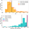 |
Fig. 1. Histograms of HR and ⟨Hk/H⟩ for all the events listed in Table A.1. Top panel shows the histograms for HR (Eq. (8)) with γ = 5/3 using two different backgrounds, BG1 and BG2. The mean, median and most probable value of HR using BG1 are 1.26, 1.1, and 0.97, respectively. Using BG2, they are 1.36, 1.19, and 1.12, respectively. The histograms in the bottom panel display the ratio of Hk to H inside the MC (⟨Hk/H⟩MC) and in the backgrounds (⟨Hk/H⟩BG1, ⟨Hk/H⟩BG2), using γ = 5/3. The mean, median, and the most probable value of ⟨Hk/H⟩MC are 0.90, 0.92, and 0.94, respectively. The mean, median, and the most probable value of ⟨Hk/H⟩BG1 are 0.98 , 0.99, and 0.995, respectively and those of ⟨Hk/H⟩BG2 are 0.99, 0.99, and 0.996, respectively. The mean value of each histogram is marked by a vertical line. |
4.2. Comparing the thermal+magnetic specific energy inside MCs and the background
Having shown that the contribution from the kinetic energy term (Hk) dominates the specific energy both in the background solar wind and inside the MC, we now compare the thermal+magnetic contributions to the specific energy in the MC and the background using the metric:
![Mathematical equation: $$ \begin{aligned} C_{\mathrm{x}} \equiv \frac{\langle \epsilon \rangle _{\rm MC}}{\langle \epsilon \rangle _{\rm BG}} , \, \, \mathrm{where}\, \, \epsilon \equiv [H_{\rm th}^2\cos ^2\theta + (H_{\rm th} + H_{\rm mag})^2\sin ^2\theta ]^{1/2} \end{aligned} $$](/articles/aa/full_html/2023/01/aa43603-22/aa43603-22-eq23.gif) (9)
(9)
The values of Cx are listed in Table B.1. As mentioned previously, ⟨ ⟩MC and ⟨ ⟩BG represent averages inside the MC and the background solar wind respectively. The quantity ϵ is the thermal+magnetic contribution to the specific energy (often called the enthalpy). The thermal contribution to the specific energy in an unmagnetized fluid is well known to be γPth/(γ − 1), and the expression for ϵ (used in Eq. (9)) is written following the reasoning in Eq. (6). The histograms of Cx in Fig. 2 have a mean, median and most probable values of 27.53, 11.09, and 2.48, respectively (using BG1) and 23.91, 14.02, and 4.36, respectively (using BG2). The mean values (which are relatively high in comparison to the median and most probable value) are biased by ≈40% of events for both the backgrounds. Our results show that the thermal+magnetic specific energy inside the MC is generally higher than that of the background. If we use γ = 1.2 instead of 5/3, we find the mean, median, and the most probable values of Cx are 18.48, 8.30, and 4.70, respectively (using BG1) and 16.51, 9.89, and 3.32, respectively (using BG2). The statistical picture of Cx thus does not differ significantly when using γ = 1.2. With γ = 5/3, the mean, median, and the most probable values of ⟨Hmag/Hth⟩ inside MCs are 23.68, 14.13, and 4.78, respectively; while it is only 2.63, 1.73, and 1.10, inside BG1, respectively and then 2.84, 2.12, and 1.63 inside BG2, respectively (Fig. 3). With γ = 1.2, ⟨Hmag/Hth⟩ is smaller (in comparison to the values with γ = 5/3) both inside the MC and in the backgrounds. The mean, median and the most probable values of ⟨Hmag/Hth⟩MC are 9.87, 5.89, and 2.43, respectively; while it is 1.10, 0.72, and 0.46, respectively (for BG1) and 1.19, 0.88, and 0.59, respectively (for BG2). The enhancement of Cx inside MCs is thus primarily attributed to the magnetic fields.
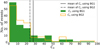 |
Fig. 2. Histograms of Cx (Eq. (9)), with γ = 5/3 and using the two backgrounds, BG1 and BG2. The mean, median, and the most probable value of Cx using BG1 are 27.53, 11.09, and 2.48, respectively while for BG2, they are 23.91, 14.02 and 4.36 respectively. The mean value for each histogram is marked by a vertical line. The maximum value shown on the x axis is limited to 100 for zooming in on the histogram peaks. |
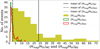 |
Fig. 3. Histograms of ⟨Hmag/Hth⟩ (with γ = 5/3) inside the MC and in the two backgrounds, BG1 and BG2, for all the events listed in Table A.1. The mean, median and the most probable value of ⟨Hmag/Hth⟩MC are 23.68, 14.13, and 4.78, respectively. The mean, median and most probable value of ⟨Hmag/Hth⟩BG1 are 2.63 , 1.73, and 1.10, respectively while for ⟨Hmag/Hth⟩BG2 they are 2.84, 2.12, and 1.63, respectively. The mean value of each histogram is marked by a vertical line. |
4.3. Comparing the thermal+magnetic pressure inside MCs and the background
There are several studies concerning the difference between the thermal+magnetic pressure Pth + Pmag inside CMEs and the ambient solar wind (Burlaga et al. 1981; Moldwin et al. 2000; Jian et al. 2005; Démoulin & Dasso 2009; Gopalswamy et al. 2015). It is often speculated that the reason ICMEs expand internally is because they are overly pressured with respect to the ambient solar wind (Scolini et al. 2019). Gopalswamy et al. (2015) and Mishra et al. (2021) examined whether ICMEs were more overly pressured during relatively weaker solar cycles, leading to more halo CMEs during such cycles. We therefore computed the following coefficient for the events in our sample using BG1 and BG2:
 (10)
(10)
where Pmag (=B2/8π) is the magnetic pressure and Pth is the thermal pressure of the plasma. The thermal pressure, Pth, includes contributions from both protons and electrons, while ⟨ ⟩MC and ⟨ ⟩BG have their usual meanings. The Cp values are listed in Table B.1 and histograms for Cp are shown in Fig. 4. The mean, median, and the most probable value for Cp using BG1 are 5.90, 4.29, and 2.39, respectively and using BG2, they are 4.76, 3.02, and 1.64, respectively. By comparison, Gopalswamy et al. (2015) found that the total pressure ratio between the MCs and the ambient solar wind is ≈3 for their set of near-Earth CMEs. The results thus suggest that the average magnetic+thermal pressure inside near-Earth MCs is appreciably higher than that of the solar wind background. The polytropic index γ has no bearing on Cp.
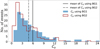 |
Fig. 4. Histograms of Cp (Eq. (10)) using two different backgrounds, BG1 and BG2. The mean, median and the most probable values of Cp with BG1 are 5.90, 4.29, and 2.39, respectively and the mean, median, and the most probable value of Cp with BG2 are 4.76, 3.02, and 1.64, respectively. The mean value for each histogram is marked by a vertical line. The maximum value shown on the x axis is limited to 24.5 in order to zoom in on the histogram peaks. |
4.4. Considering whether the excess thermal+magnetic specific energy and pressure inside MCs are correlated with near-Earth expansion and propagation speeds
Just as several past studies have questioned whether the excess pressure inside ICMEs leads to their expansion (see e.g., von Steiger & Richardson 2006; Scolini et al. 2019; Démoulin & Dasso 2009; Verbeke et al. 2022), it is natural to question whether the enhanced thermal+magnetic specific energy inside MCs results in their expansion. We compute the MC expansion speed (Nieves-Chinchilla et al. 2018) as:
 (11)
(11)
for each MC in our sample. The quantities vs and ve are the speeds at the start and at the end of the MC respectively. Figure 5 shows an example of a linear fit that is used to compute vs, ve, and consequently, vexp. We note that vexp for ≈20% of MCs in our sample is negative; that is, they contract rather than expand. Figure 6 shows scatterplots between Cx (estimated using both BG1 and BG2) and the near-Earth MC propagation speed, ⟨v⟩MC (panel a), and, vexp (panel b), for expanding MCs (i.e., those for which we have vexp > 0). The linear correlation coefficient (r) between Cx and the MC propagation speed (⟨v⟩MC) is 0.43, with a p-value of 3.5 × 10⁻⁸ with BG1 and r = 0.51, with p = 1.8 × 10⁻¹¹ with BG2. The linear correlation coefficient (r) between Cx and vexp for the expanding events is 0.50 and the corresponding p-value is 5.73 × 10⁻⁹ (using BG1) and r = 0.63, with p = 1.9 × 10⁻¹⁴ (using BG2). The correlation coefficient between Cx and vexp/⟨v⟩ (considering only events with positive vexp), namely, r = 0.40, with a p-value 7.8 × 10⁻⁶ for BG1 and r = 0.50, with p = 1.2 × 10⁻⁸ for BG2. Our findings suggest that Cx is only moderately correlated with the near-Earth MC propagation and expansion speed. The low values for p in all the cases indicate a high statistical significance for these results.
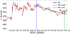 |
Fig. 5. Velocity (v) profile as a function of time for event 54 in our dataset (Table A.1). The start time (ts) and end time (te) of the MC are marked by blue and green dashed lines, respectively. The black solid line shows a linear fit to v. vs and ve denote the value of the fit at ts and te, respectively. We compute the MC expansion speed, vexp (Eq. (11)), using vs and ve. |
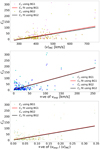 |
Fig. 6. Scatter plots of Cx with MC propagation and expansion speeds for all the events listed in Table A.1. The top panel is the scatterplot between Cx (estimated using γ = 5/3; as in Eq. (9)) and the MC propagation speed (⟨v⟩MC). The correlation coefficient between Cx and ⟨v⟩MC are r = 0.43, with p = 3.5 × 10⁻⁸ (for BG1) and r = 0.51, with p = 1.8 × 10⁻¹¹ (for BG2). The equation of the fitted lines corresponding to BG1 and BG2 are y = 0.25x − 75.65 and y = 0.24x − 73.28, respectively. The middle panel is the scatter plot between Cx (computed using γ = 5/3) and the MC expansion speed (vexp), only for events with vexp > 0. The correlation coefficients are r = 0.50, with p = 5.73 × 10⁻⁹ for BG1 and r = 0.63, with p = 1.9 × 10⁻¹⁴ for BG2. The equation of fitted lines are y = 0.72x + 4.82 and y = 0.73x + 2.73 corresponding to BG1 and BG2, respectively. The bottom panel is the scatter plot between Cx (calculated using γ = 5/3) and vexp/⟨v⟩MC (only for events with vexp > 0). The correlation coefficients are r = 0.40, with p = 7.8 × 10⁻⁶(for BG1) and r = 0.50, with p = 1.2 × 10⁻⁸(for BG2). The equation of the fitted lines are y = 342.6x + 3.36 (for BG1) and y = 341.71x + 1.46 (for BG2). The small p-values imply a high statistical confidence in computing the r values in all three cases. |
We next study if and how the overpressure parameter Cp may be correlated with the near-Earth MC expansion and propagation speeds. Panel a of Fig. 7 shows the scatter plot between Cp (using both BG1 and BG2) and the MC propagation speed. The correlation is low (r = 0.18, p-value = 2 × 10⁻² using BG1 and r = 0.15, p = 5 × 10⁻² using BG2). The correlation between Cp and the MC expansion speed of the expanding MCs (vexp > 0) is also low (see panel b of Fig. 7; r = 0.25, p-value = 2 × 10⁻³ using BG1 and r = 0.25 with p = 5 × 10⁻³). Finally, we note that the correlation coefficients between Cp and vexp/⟨v⟩MC for the expanding MCs (see panel c of Fig. 7) are r = 0.23 and the p-value is 6 × 10⁻³ for BG1 and r = 0.22, with p = 10−3 for BG2. Evidently, Cp is rather poorly correlated with MC expansion and propagation speeds. This might be because we are using speeds measured at the position of the WIND observation, whereas most of the CME expansion probably occurs closer to the Sun (Verbeke et al. 2022).
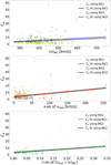 |
Fig. 7. Scatter plots of Cp with MC propagation and expansion speeds for all the events listed in Table A.1. The top panel is the scatter plot between Cp (Eq. (10) and the MC propagation speed (⟨v⟩MC). The correlation coefficient between Cp and ⟨v⟩MC is r = 0.18, with p = 2 × 10⁻² (for BG1) and r = 0.15, with p = 5 × 10⁻² (for BG2). The equation of the fitted lines corresponding to BG1 and BG2 are y = 0.01x − 0.004 and y = 0.01x − 0.1, respectively. The middle panel is the scatter plot between Cp and the MC expansion speed (vexp), only for events with vexp > 0. The correlation coefficients are r = 0.25, with p = 2 × 10⁻³ for BG1 and r = 0.25, with p = 5 × 10⁻³ for BG2. The equation of the fitted lines are y = 0.05x + 4.5 and y = 0.05x + 3.26, for BG1 and BG2, respectively. The bottom panel is the scatter plot between Cp and vexp/⟨v⟩MC, only for events with vexp > 0. The correlation coefficients are r = 0.23, with p = 6 × 10⁻³ (for BG1) and r = 0.22, with p = 10−3 (for BG2). The equation of the fitted lines are y = 25.3x + 4.30 (for BG1) and y = 25.78x + 3.02 (for BG2). The small p-values indicate a sufficiently high statistical confidence in estimating the r values for all three cases. |
5. Considering whether the excess thermal+magnetic specific energy in MCs may make them appear “rigid”
The main results we have obtained thus far are that (i) the total specific energy inside the MC is roughly equivalent to that of the background; and (ii) the sum of the thermal and magnetic (specific) energies is higher inside the MC as compared to the background. By way of attempting to understand point (ii) better, we define the following coefficient:
 (12)
(12)
where ϵ is defined in Eq. (9) and u ≡ v − ⟨v⟩MC is the solar wind velocity in the frame of the MC, while the other notations carry their usual meanings. The quantity ⟨(1/2)u2⟩BG denotes the specific kinetic energy of the oncoming solar wind incident on the MC, as discerned by an observer moving with the average MC speed. The quantity Cr (Eq. (12)) thus compares the excess thermal+magnetic specific energy in the MC (relative to the background) with the specific kinetic energy of the solar wind impinging on it. If Cr ≳ 1, it means that the excess thermal+magnetic specific energy in the MC is greater than the specific kinetic energy of the oncoming solar wind – suggesting that the MC can resist deformation by the solar wind, somewhat akin to the case of a rigid body. One way to understand Cr is as follows: we can imagine an inflated balloon placed in a stream of cold air. There are no magnetic fields, and so Hmag = 0. Since the air stream is cold, ⟨Hth⟩BG is zero and the only term in the numerator of Eq. (12) is ⟨Hth⟩MC. The metric Cr thus compares the thermal specific energy due of the gas inside the balloon with the specific kinetic energy of the cold air stream incident on it. If Cr ≳ 1, the balloon can resist deformation due to the incident air stream relatively better (i.e., it behaves more like a well-inflated soccer ball) and vice versa.
The Cr values for all the events in our dataset are listed in Table B.1. The histogram of Cr for all the events using γ = 5/3 and both the backgrounds (BG1 and BG2) is shown in Fig. 8. With BG1, we find that the mean, median, and most probable values of Cr histogram are 7.61, 3.33, and 1.16, respectively, with 81% of the events having Cr ≥ 1. Using BG2, the mean, median, and most probable values are 8.65, 4.66, and 2.25, respectively, and with 89.5% of the events having Cr ≥ 1. If we assume γ = 1.2 (instead of 5/3), the mean, median, and most probable values of Cr are 8.09, 3.55, and 1.12, respectively with BG1, and 9.50, 5.29, and 2.29, respectively with BG2. The choice of γ does not affect our results substantially.
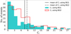 |
Fig. 8. Histograms of Cr (Eq. (12)) with γ = 5/3 using both the backgrounds (BG1 and BG2). The mean, median, and the most probable values of Cr are 7.61, 3.33, and 1.16, respectively for BG1 and 8.65, 4.65, and 2.25, respectively for BG2. The mean value of each histogram is marked by a vertical line. The maximum value shown on the x axis is limited to 28 for zooming in on the histogram peaks. |
Furthermore, the magnetic energy is typically higher than the thermal energy inside MCs, (Fig. 3) suggesting that CME magnetic fields are primarily responsible for Cr ≥ 1. Our findings are in keeping with those of Lynnyk et al. (2011) who stated that “if the magnetic field inside the ICME/MC is much stronger than that in the ambient solar wind, the ICME/MC cross-section is closer to circular.” Thus, MCs with more circular cross-sections are probably those that are relatively more rigid; namely, those that are probably characterized by Cr ≥ 1, and that have resisted deformation by the solar wind.
An issue related to the rigidity of MCs is the widely used CME aerodynamic drag law (Cargill 2004; Vršnak et al. 2009, 2013)
 (13)
(13)
which is a hydrodynamic drag law applicable to high Reynolds number flows past solid or rigid bodies (Landau & Lifshitz 1987). In Eq. (13), FD is the drag force, u is the velocity of the background fluid as viewed by an observer comoving with the body, A is the cross-sectional area subtended by the body to the flow, ρ is the mass density of the background fluid, and CD is a dimensionless proportionality constant. By contrast, the high Reynolds number drag law for flows past deformable bubbles resemble FD ∝ u (Landau & Lifshitz 1987; Moore 1959, 1963; Kang & Leal 1988). Although the FD ∝ u resembles the Stokes law, which is applicable for laminar or low Reynolds number flows past solid bodies, it is, in fact a high Reynolds number law for flows past deformable bubbles. Bubbles are distinct from solid bodies in that the total velocity does not vanish on their surface, as it does for solid bodies. We note that some studies of CME dynamics have indeed adopted FD ∝ u (Vršnak & Gopalswamy 2002; Maloney & Gallagher 2010). Although the form of the widely adopted CME aerodynamic drag law arises from an amalgamation of several MHD effects (Lin & Chen 2022), the simplest interpretation of Eq. (13) is still that of a high Reynolds number, solid or rigid body law. Our finding Cr ≳ 1 (for over 89% of the MCs we study) might be a possible justification for the solid body premise, even for CMEs, which are obviously far from solid bodies in the usual sense of the word.
6. Conclusions and discussion
Generally, CME evolution through the heliosphere is thought to be strongly influenced by the difference in the (thermal+magnetic) pressures inside the CME and outside of it, that is, in the ambient solar wind. In this study we compare the average value of the total specific energy, H (Eq. (6)), inside MCs and the background solar wind using the near-Earth in situ data from the WIND spacecraft for a set of 152 well observed MCs. The quantity H contains contributions from the kinetic energy due to the bulk flow (Hk), the thermal energy (Hth), and the magnetic energy (Hmag). We also compare the thermal+magnetic pressure inside MCs with the background solar wind. We use two different ambient solar wind backgrounds for our comparisons and also use two different values for the polytropic index γ. Our main conclusions are as follows:
-
The average value of H inside MCs: ⟨H⟩MC is approximately equivalent to the average value in the ambient solar wind ⟨H⟩BG (Sect. 4.1, Fig. 1). The bulk-flow kinetic energy contribution is Hk ≈ H, both inside the MCs and in the ambient solar wind. This is the primary reason for the following approximation: ⟨H⟩MC ≈ ⟨H⟩BG.
-
The average thermal+magnetic specific energy inside near-Earth MCs substantially exceeds that of the background solar wind (Sect. 4.2). Similarly, the average Pth + Pmag inside near-Earth MCs is greater than that in the solar wind background (Sect. 4.3). These conclusions are broadly consistent with the findings of Gopalswamy et al. (2015) and Mishra et al. (2021).
-
We find that the excess thermal+magnetic energy inside MCs is moderately correlated with MC near-Earth propagation and expansion speeds, while the correlation is rather poor for the excess thermal+magnetic pressure (Sect. 4.4). In summary, neither the excess enthalpy nor total pressure seem to be well correlated with the near-Earth MC propagation nor the expansion speeds. This might be because most of the expansion occurs closer to the Sun (Odstrčil & Pizzo 1999; Gopalswamy et al. 2014; Verbeke et al. 2022) and/or because magnetic field rearrangement is the primary reason for expansion (Kumar & Rust 1996).
-
We find that the excess thermal+magnetic specific energy inside MCs ≳ the specific kinetic energy of the solar wind impinging on them for 81–89% of the events we study (Sect. 5). This suggests the ways in which MCs might able to resist deformation by the solar wind. Furthermore, this might suggest a justification for the popular “rigid body” CME aerodynamic drag law (Eq. (13).
Our results are based solely on in situ data at the position of the WIND measurements (i.e., at 1 AU). It would be interesting to carry out similar calculations using in-situ data closer to the Sun from the PSP (Weiss et al. 2020; Nieves-Chinchilla et al. 2022), which would yield potential new insights on the evolution of CMEs throughout the heliosphere.
Acknowledgments
DB acknowledges the PhD studentship from Indian Institute of Science Education and Research, Pune. We acknowledge a detailed review by an anonymous referee that helped us improve the manuscript.
References
- Bhattacharjee, D., Subramanian, P., Bothmer, V., Nieves-Chinchilla, T., & Vourlidas, A. 2022, Sol. Phys., 297, 45 [NASA ADS] [CrossRef] [Google Scholar]
- Bothmer, V., & Schwenn, R. 1998, AnGeo, 16, 1 [NASA ADS] [CrossRef] [Google Scholar]
- Boyd, T. J. M., & Sanderson, J. J. 2003, phpl.book, 544 [Google Scholar]
- Burlaga, L., Sittler, E., Mariani, F., & Schwenn, R. 1981, J. Geophys. Res., 86, 6673 [Google Scholar]
- Cargill, P. J. 2004, Sol. Phys., 221, 135 [Google Scholar]
- Cargill, P. J., & Schmidt, J. M. 2002, Ann. Geophys., 20, 879 [Google Scholar]
- Cargill, P. J., Chen, J., Spicer, D. S., et al. 1995, Geophys. Res. Lett., 22, 647 [NASA ADS] [CrossRef] [Google Scholar]
- Chané, E., Schmieder, B., Dasso, S., et al. 2021, A&A, 647, A149 [NASA ADS] [CrossRef] [EDP Sciences] [Google Scholar]
- Chen, J. 1996, J. Geophys. Res., 101, 27499 [NASA ADS] [CrossRef] [Google Scholar]
- Chen, P. F. 2011, Liv. Rev. Sol. Phys., 8, 1 [Google Scholar]
- Chen, J., & Garren, D. A. 1993, Geophys. Res. Lett., 20, 2319 [NASA ADS] [CrossRef] [Google Scholar]
- Dakeyo, J. B., Maksimovic, M., Démoulin, P., Halekas, J., & Stevens, M. L. 2022, ArXiv e-prints [arXiv:2207.03898] [Google Scholar]
- Démoulin, P., & Dasso, S. 2009, A&A, 498, 551 [Google Scholar]
- Davies, E. E., Möstl, C., Owens, M. J., et al. 2021, A&A, 656, A2 [NASA ADS] [CrossRef] [EDP Sciences] [Google Scholar]
- Dasso, S., Nakwacki, M. S., Démoulin, P., & Mandrini, C. H. 2007, Sol. Phys., 244, 115 [Google Scholar]
- Forsyth, R. J., Bothmer, V., Cid, C., et al. 2006, Space Sci. Rev., 123, 383 [NASA ADS] [CrossRef] [Google Scholar]
- Gopalswamy, N., Akiyama, S., Yashiro, S., et al. 2014, Geophys. Res. Lett., 41, 2673 [NASA ADS] [CrossRef] [Google Scholar]
- Gopalswamy, N., Yashiro, S., Xie, H., Akiyama, S., & Mäkelä, P. 2015, J. Geophys. Res. (Space Phys.), 120, 9221 [NASA ADS] [CrossRef] [Google Scholar]
- Groth, C. P. T., De Zeeuw, D. L., Gombosi, T. I., & Powell, K. G. 2000, J. Geophys. Res., 105, 25053 [NASA ADS] [CrossRef] [Google Scholar]
- Guo, J., Feng, X., Emery, B. A., et al. 2011, J. Geophys. Res. (Space Phys.), 116, A05106 [NASA ADS] [Google Scholar]
- Hidalgo, M. A. 2003, J. Geophys. Res., 108, 1320 [NASA ADS] [CrossRef] [Google Scholar]
- Jian, L., Russell, C. T., Gosling, J. T., & Luhmann, J. G. 2005, Sol. Phys., 592, 731 [Google Scholar]
- Jian, L., Russell, C. T., Luhmann, J. G., & Skoug, R. M. 2008, AdSpR, 41, 259 [NASA ADS] [Google Scholar]
- Kang, I. S., & Leal, L. G. 1988, Phys. Fluids, 31, 233 [NASA ADS] [CrossRef] [Google Scholar]
- Kassa Dagnew, F., Gopalswamy, N., Belay Tessema, S., Akiyama, S., & Yashiro, S. 2022, ApJ, accepted [arXiv:2208.03536] [Google Scholar]
- Keppens, R., Teunissen, J., Xia, C., & Porth, O. 2020, CAMWA, accepted [arXiv:2004.03275] [Google Scholar]
- Kilpua, E., Isavnin, A., Vourlidas, A., Koskinen, H., & Rodriguez, L. 2013, EGU General Assembly Conference Abstracts [Google Scholar]
- Klein, L. W., & Burlaga, L. F. 1982, J. Geophys. Res., 87, 613 [Google Scholar]
- Klein, K. G., Howes, G. G., TenBarge, J. M., et al. 2012, ApJ, 755, 159 [NASA ADS] [CrossRef] [Google Scholar]
- Kumar, A., & Rust, D. M. 1996, J. Geophys. Res., 101, 15667 [Google Scholar]
- Kundu, P. K., & Cohen, I. M. 2008, Fluid Mechanics, 4th edn. (Cambridge: Academic Press) [Google Scholar]
- Kulsrud, R. M. 2005, Plasma Physics for Astrophysics (Princeton: Princeton University Press) [Google Scholar]
- Landau, L. D., & Lifshitz, E. M. 1987, Fluid Mechanics, 2nd edn. (Pergamon) [Google Scholar]
- Lepping, R. P., Berdichevsky, D. B., Szabo, A., Arqueros, C., & Lazarus, A. J. 2003, Sol. Phys., 212, 425 [NASA ADS] [CrossRef] [Google Scholar]
- Lin, C.-H., & Chen, J. 2022, J. Geophys. Res. (Space Phys.), 127 [Google Scholar]
- Linker, J. A., Mikić, Z., Biesecker, D. A., et al. 1999, J. Geophys. Res., 104, 9809 [NASA ADS] [CrossRef] [Google Scholar]
- Lionello, R., Downs, C., Linker, J. A., et al. 2013, ApJ, 777, 76 [NASA ADS] [CrossRef] [Google Scholar]
- Lugaz, N., & Roussev, I. I. 2011, J. Atmos. Solar-Terrest. Phys., 73, 1187 [NASA ADS] [CrossRef] [Google Scholar]
- Lugaz, N., Hernandez-Charpak, J. N., Roussev, I. I., et al. 2010, ApJ, 715, 493 [NASA ADS] [CrossRef] [Google Scholar]
- Lugaz, N., Salman, T. M., Winslow, R. M., et al. 2020, ApJ, 899, 11 [Google Scholar]
- Lynnyk, A., Šafránková, J., Němeček, Z., & Richardson, J. D. 2011, Planet Space. Sci., 59, 840 [CrossRef] [Google Scholar]
- Maloney, S. A., & Gallagher, P. T. 2010, ApJ, 724, L127 [NASA ADS] [CrossRef] [Google Scholar]
- Manchester, W. B., Gombosi, T. I., Roussev, I., et al. 2004, J. Geophys. Res., 109, A01102 [NASA ADS] [Google Scholar]
- Marsch, E., & Tu, C.-Y. 1990, J. Geophys. Res., 95, 11945 [NASA ADS] [CrossRef] [Google Scholar]
- Mishra, W., & Wang, Y. 2018, ApJ, 865, 50 [NASA ADS] [CrossRef] [Google Scholar]
- Mishra, W., Doshi, U., & Srivastava, N. 2021, Front. Astron. Space Sci., 8, 142 [NASA ADS] [CrossRef] [Google Scholar]
- Moldwin, M. B., Ford, S., Lepping, R., Slavin, J., & Szabo, A. 2000, Geophys. Res. Lett., 27, 57 [NASA ADS] [CrossRef] [Google Scholar]
- Moore, D. W. 1959, J. Fluid Mech., 6, 113 [NASA ADS] [CrossRef] [Google Scholar]
- Moore, D. W. 1963, J. Fluid Mech., 16, 161 [NASA ADS] [CrossRef] [Google Scholar]
- Nicolaou, G., Livadiotis, G., Wicks, R. T., Verscharen, D., & Maruca, B. A. 2020, ApJ, 901, 26 [CrossRef] [Google Scholar]
- Nieves-Chinchilla, T., Colaninno, R., Vourlidas, A., et al. 2012, J. Geophys. Res., 117, A06106 [NASA ADS] [Google Scholar]
- Nieves-Chinchilla, T., Linton, M. G., Hidalgo, M. A., et al. 2016, ApJ, 823, 27 [NASA ADS] [CrossRef] [Google Scholar]
- Nieves-Chinchilla, T., Vourlidas, A., Raymond, J. C., et al. 2018, Sol. Phys., 293, 25 [NASA ADS] [CrossRef] [Google Scholar]
- Nieves-Chinchilla, T., Jian, L. K., Balmaceda, L., et al. 2019, Sol. Phys., 294, 89 [Google Scholar]
- Nieves-Chinchilla, T., Alzate, N., Cremades, H., et al. 2022, ApJ, 930, 88 [NASA ADS] [CrossRef] [Google Scholar]
- Odstrčil, D., & Pizzo, V. J. 1999, J. Geophys. Res., 104, 493 [CrossRef] [Google Scholar]
- Odstrcil, D., & Pizzo, V. J. 2009, Sol. Phys., 259, 297 [Google Scholar]
- Parker, E. N. 2009, Climate and Weather of the Sun-earth System (CAWSES), 23 [Google Scholar]
- Richardson, I. G., & Cane, H. V. 2010, Sol. Phys., 264, 189 [NASA ADS] [CrossRef] [Google Scholar]
- Rollett, T., Möstl, C., Temmer, M., Veronig, A., & Farrugia, C. J. 2012, Solar Heliospheric and INterplanetary Environment (SHINE 2012) [Google Scholar]
- Russell, C. T., Shinde, A. A., & Jian, L. 2005, AdSpR, 35, 2178 [NASA ADS] [Google Scholar]
- Sachdeva, N., Subramanian, P., Colaninno, R., & Vourlidas, A. 2015, ApJ, 809, 158 [NASA ADS] [CrossRef] [Google Scholar]
- Sachdeva, N., Subramanian, P., Vourlidas, A., & Bothmer, V. 2017, Sol. Phys., 292, 118 [Google Scholar]
- Savani, N. P., Owens, M. J., Rouillard, A. P., Forsyth, R. J., & Davies, J. A. 2010, ApJ, 714, L128 [NASA ADS] [CrossRef] [Google Scholar]
- Savani, N. P., Owens, M. J., Rouillard, A. P., et al. 2011, ApJ, 732, 117 [NASA ADS] [CrossRef] [Google Scholar]
- Scolini, C., Rodriguez, L., Mierla, M., Pomoell, J., & Poedts, S. 2019, A&A, 626, A122 [NASA ADS] [CrossRef] [EDP Sciences] [Google Scholar]
- Spruit, H. C. 2013, ArXiv e-prints [arXiv:1301.5572] [Google Scholar]
- St. Cyr, O. C., Plunkett, S. P., Michels, D. J., et al. 2000, J. Geophys. Res., 105, 18169 [CrossRef] [Google Scholar]
- Tóth, G., van der Holst, B., Sokolov, I. V., et al. 2012, J. Comput. Phys., 231, 870 [Google Scholar]
- Temmer, M. 2021, Liv. Rev. Sol. Phys., 18, 4 [NASA ADS] [CrossRef] [Google Scholar]
- Verbeke, C., Schmieder, B., Démoulin, P., et al. 2022, AdSpR, 70, 1663 [NASA ADS] [Google Scholar]
- von Steiger, R., & Richardson, J. D. 2006, Space Sci. Rev., 123, 111 [NASA ADS] [CrossRef] [Google Scholar]
- Vršnak, B., & Gopalswamy, N. 2002, J. Geophys. Res. (Space Phys.), 107, 1019 [Google Scholar]
- Vršnak, B., Vrbanec, D., Čalogović, J., et al. 2009, Universal Heliophysical Processes, 271 [Google Scholar]
- Vršnak, B., Žic, T., Vrbanec, D., et al. 2013, Sol. Phys., 285, 295 [Google Scholar]
- Wang, C., & Richardson, J. D. 2004, J. Geophys. Res., 109, A06104 [NASA ADS] [Google Scholar]
- Webb, D. F., Howard, T. A., Fry, C. D., et al. 2009, Sol. Phys., 256, 239 [NASA ADS] [CrossRef] [Google Scholar]
- Weber, E. J., & Davis, L. 1967, ApJ, 148, 217 [Google Scholar]
- Weiss, A., Möstl, C., Nieves-Chinchilla, T., et al. 2020, EGU General Assembly Conference Abstracts [Google Scholar]
- Xie, H., Ofman, L., & Lawrence, G. 2004, J. Geophys. Res. (Space Phys.), 109, A03109 [NASA ADS] [Google Scholar]
Appendix A: Data table
List of the 152 WIND ICME events we use in this study. The arrival date and time of the ICME at the position of WIND measurement and the arrival and departure dates & times of the associated magnetic clouds (MCs) are taken from the WIND ICME catalog (https://wind.nasa.gov/ICMEindex.php). The 14 events marked with and asterisk (*) coincide with the near-Earth counterparts of 14 CMEs listed in Sachdeva et al. (2017).
Appendix B: List of Cx, Cp, and Cr for all events in our dataset
Cx (Equation 9), Cp (Equation 10), and Cr (Equation 12) for all events in the dataset. The 14 events marked with and asterisk (*) coincide with the near-Earth counterparts of 14 CMEs listed in Sachdeva et al. (2017).
All Tables
List of the 152 WIND ICME events we use in this study. The arrival date and time of the ICME at the position of WIND measurement and the arrival and departure dates & times of the associated magnetic clouds (MCs) are taken from the WIND ICME catalog (https://wind.nasa.gov/ICMEindex.php). The 14 events marked with and asterisk (*) coincide with the near-Earth counterparts of 14 CMEs listed in Sachdeva et al. (2017).
Cx (Equation 9), Cp (Equation 10), and Cr (Equation 12) for all events in the dataset. The 14 events marked with and asterisk (*) coincide with the near-Earth counterparts of 14 CMEs listed in Sachdeva et al. (2017).
All Figures
|
Fig. 1. Histograms of HR and ⟨Hk/H⟩ for all the events listed in Table A.1. Top panel shows the histograms for HR (Eq. (8)) with γ = 5/3 using two different backgrounds, BG1 and BG2. The mean, median and most probable value of HR using BG1 are 1.26, 1.1, and 0.97, respectively. Using BG2, they are 1.36, 1.19, and 1.12, respectively. The histograms in the bottom panel display the ratio of Hk to H inside the MC (⟨Hk/H⟩MC) and in the backgrounds (⟨Hk/H⟩BG1, ⟨Hk/H⟩BG2), using γ = 5/3. The mean, median, and the most probable value of ⟨Hk/H⟩MC are 0.90, 0.92, and 0.94, respectively. The mean, median, and the most probable value of ⟨Hk/H⟩BG1 are 0.98 , 0.99, and 0.995, respectively and those of ⟨Hk/H⟩BG2 are 0.99, 0.99, and 0.996, respectively. The mean value of each histogram is marked by a vertical line. |
| In the text | |
|
Fig. 2. Histograms of Cx (Eq. (9)), with γ = 5/3 and using the two backgrounds, BG1 and BG2. The mean, median, and the most probable value of Cx using BG1 are 27.53, 11.09, and 2.48, respectively while for BG2, they are 23.91, 14.02 and 4.36 respectively. The mean value for each histogram is marked by a vertical line. The maximum value shown on the x axis is limited to 100 for zooming in on the histogram peaks. |
| In the text | |
|
Fig. 3. Histograms of ⟨Hmag/Hth⟩ (with γ = 5/3) inside the MC and in the two backgrounds, BG1 and BG2, for all the events listed in Table A.1. The mean, median and the most probable value of ⟨Hmag/Hth⟩MC are 23.68, 14.13, and 4.78, respectively. The mean, median and most probable value of ⟨Hmag/Hth⟩BG1 are 2.63 , 1.73, and 1.10, respectively while for ⟨Hmag/Hth⟩BG2 they are 2.84, 2.12, and 1.63, respectively. The mean value of each histogram is marked by a vertical line. |
| In the text | |
|
Fig. 4. Histograms of Cp (Eq. (10)) using two different backgrounds, BG1 and BG2. The mean, median and the most probable values of Cp with BG1 are 5.90, 4.29, and 2.39, respectively and the mean, median, and the most probable value of Cp with BG2 are 4.76, 3.02, and 1.64, respectively. The mean value for each histogram is marked by a vertical line. The maximum value shown on the x axis is limited to 24.5 in order to zoom in on the histogram peaks. |
| In the text | |
|
Fig. 5. Velocity (v) profile as a function of time for event 54 in our dataset (Table A.1). The start time (ts) and end time (te) of the MC are marked by blue and green dashed lines, respectively. The black solid line shows a linear fit to v. vs and ve denote the value of the fit at ts and te, respectively. We compute the MC expansion speed, vexp (Eq. (11)), using vs and ve. |
| In the text | |
|
Fig. 6. Scatter plots of Cx with MC propagation and expansion speeds for all the events listed in Table A.1. The top panel is the scatterplot between Cx (estimated using γ = 5/3; as in Eq. (9)) and the MC propagation speed (⟨v⟩MC). The correlation coefficient between Cx and ⟨v⟩MC are r = 0.43, with p = 3.5 × 10⁻⁸ (for BG1) and r = 0.51, with p = 1.8 × 10⁻¹¹ (for BG2). The equation of the fitted lines corresponding to BG1 and BG2 are y = 0.25x − 75.65 and y = 0.24x − 73.28, respectively. The middle panel is the scatter plot between Cx (computed using γ = 5/3) and the MC expansion speed (vexp), only for events with vexp > 0. The correlation coefficients are r = 0.50, with p = 5.73 × 10⁻⁹ for BG1 and r = 0.63, with p = 1.9 × 10⁻¹⁴ for BG2. The equation of fitted lines are y = 0.72x + 4.82 and y = 0.73x + 2.73 corresponding to BG1 and BG2, respectively. The bottom panel is the scatter plot between Cx (calculated using γ = 5/3) and vexp/⟨v⟩MC (only for events with vexp > 0). The correlation coefficients are r = 0.40, with p = 7.8 × 10⁻⁶(for BG1) and r = 0.50, with p = 1.2 × 10⁻⁸(for BG2). The equation of the fitted lines are y = 342.6x + 3.36 (for BG1) and y = 341.71x + 1.46 (for BG2). The small p-values imply a high statistical confidence in computing the r values in all three cases. |
| In the text | |
|
Fig. 7. Scatter plots of Cp with MC propagation and expansion speeds for all the events listed in Table A.1. The top panel is the scatter plot between Cp (Eq. (10) and the MC propagation speed (⟨v⟩MC). The correlation coefficient between Cp and ⟨v⟩MC is r = 0.18, with p = 2 × 10⁻² (for BG1) and r = 0.15, with p = 5 × 10⁻² (for BG2). The equation of the fitted lines corresponding to BG1 and BG2 are y = 0.01x − 0.004 and y = 0.01x − 0.1, respectively. The middle panel is the scatter plot between Cp and the MC expansion speed (vexp), only for events with vexp > 0. The correlation coefficients are r = 0.25, with p = 2 × 10⁻³ for BG1 and r = 0.25, with p = 5 × 10⁻³ for BG2. The equation of the fitted lines are y = 0.05x + 4.5 and y = 0.05x + 3.26, for BG1 and BG2, respectively. The bottom panel is the scatter plot between Cp and vexp/⟨v⟩MC, only for events with vexp > 0. The correlation coefficients are r = 0.23, with p = 6 × 10⁻³ (for BG1) and r = 0.22, with p = 10−3 (for BG2). The equation of the fitted lines are y = 25.3x + 4.30 (for BG1) and y = 25.78x + 3.02 (for BG2). The small p-values indicate a sufficiently high statistical confidence in estimating the r values for all three cases. |
| In the text | |
|
Fig. 8. Histograms of Cr (Eq. (12)) with γ = 5/3 using both the backgrounds (BG1 and BG2). The mean, median, and the most probable values of Cr are 7.61, 3.33, and 1.16, respectively for BG1 and 8.65, 4.65, and 2.25, respectively for BG2. The mean value of each histogram is marked by a vertical line. The maximum value shown on the x axis is limited to 28 for zooming in on the histogram peaks. |
| In the text | |
Current usage metrics show cumulative count of Article Views (full-text article views including HTML views, PDF and ePub downloads, according to the available data) and Abstracts Views on Vision4Press platform.
Data correspond to usage on the plateform after 2015. The current usage metrics is available 48-96 hours after online publication and is updated daily on week days.
Initial download of the metrics may take a while.