| Issue |
A&A
Volume 580, August 2015
|
|
|---|---|---|
| Article Number | A126 | |
| Number of page(s) | 26 | |
| Section | Galactic structure, stellar clusters and populations | |
| DOI | https://doi.org/10.1051/0004-6361/201424171 | |
| Published online | 18 August 2015 | |
Online material
Appendix A: Gas in the MW disk
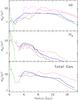 |
Fig. A.1
Surface density profiles of atomic hydrogen HI (top), molecular hydrogen H2 (middle) and total gas ΣG = 1.4 (HI+H2) (bottom). Disk data (beyond 2 kpc) are from: Dame (1993), solid; Olling & Merrifield (2001), dotted ; and Nakanishi & Sofue (2003, 2006), dashed. The dot-dashed curve in the HI panel corresponds to data from Kalberla & Dedes (2008) and in the H2 panel to data from Pohl et al. (2008). Bulge data (inner 2 kpc) in all panels are from Ferrière (2001). |
| Open with DEXTER | |
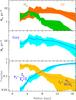 |
Fig. A.2
Average profiles of the previous figure. Top: atomic and molecular hydrogen; middle: total gas ; bottom: fractions of gas (solid) and molecular gas (dashed). For the latter panel, an exponential stellar density profile with a scale-length of 2.3 kpc normalised to Σ∗(R = 8 kpc) = 38 M⊙/pc2 is adopted, while the molecular fraction is evaluated with the formalism of Appendix B. |
| Open with DEXTER | |
In Fig. A.1 we present the data adopted for the gas profiles of the MW. Atomic hydrogen (HI) is displayed in the upper panel and molecular hydrogen (H2) in the middle panel. In both cases, data are from Dame (1993), Olling & Merrifield (2001) and Nakanishi & Sofue (2003). The data have been rescaled to a distance of R0 = 8 kpc of the Sun from the Galactic centre. The bottom panel shows the total gas surface density ΣG = 1.4(HI+H2), where the factor 1.4 accounts for the presence of ~28% of He. In all panels, the data for the inner Galaxy (R< 2 kpc) are from Ferrière et al. (2007) and they are provided for completeness, since the evolution of the bulge is not studied here.
Despite systematic differences in the data, the gas profiles in the three panels of Fig. A.1 have some common features:
-
The HI profile is essentially flat in the 4−12 kpc region.
-
The H2 profile displays the well known “molecular ring” in the 4−5 kpc region and declines rapidly outwards.
-
The total gas profile is approximately constant (or slowly declining outwards) in the 4−12 kpc region; it declines more rapidly inside the molecular ring, as well as outside 13 kpc, where it has a scalelength of 3.75 kpc (Kalberla & Dedes 2008).
To minimize systematic uncertainties in the following, we adopt the averages of the aforementioned observed profiles as a function of galactocentric radius as the “reference gaseous profiles” for the MW disk. They appear in Fig. A.2, top panel for HI and H2 and middle panel for the total gas. As a typical uncertainty in each radius, we adopt either 50% of the average value (typical statistical uncertainty in e.g. Nakanishi & Sofue 2006) or half the difference between the minimum and maximum values in each radial bin (whichever is larger). The resulting values for the total galactic content of HI, H2 and gas appear in Table A.1. The derived masses appear lower than the ones obtained with the mass model of the ISM in the Milky Way of Misiriotis et al. (2006), who find total masses of MH2 = 1.3 × 10⁹M⊙ and MHI = 8.2 × 10⁹, but they match the FIR emission of the whole Galaxy, whereas we quote here results for the 2−19 kpc range. There are considerable amounts of HI in the outer disk, as discussed in e.g. Kalberla & Dedes (2008).
Gas in the MW disk (2−19 kpc) in 109M⊙.
We find then that the Galactic disk has a total gaseous content of ~ 8.2 ± 3.5 × 10⁹M⊙ in the 2−19 kpc range. Assuming an exponential stellar profile with a scalelength Rd = 2.3 kpc for the MW disk, normalised to a local (R0 = 8 kpc) surface density Σ∗ ,0 = 38M⊙/pc2 (Flynn et al. 2006), we find a total stellar mass of 3.2 × 10¹⁰M⊙ and obtain the radial profile of the gas fraction ![]() . It is displayed in the bottom panel of Fig. A.2 and it is a monotonically increasing function of radius. Integrating as before the gaseous and stellar profiles over the disk region between 2 and 19 kpc we find an average gas fraction of σG = 0.20 ± 0.05 for the disk. If the bulge (of stellar mass ~1.5 × 10¹⁰M⊙ and negligible gas) is also included, the gas fraction of the MW is found to be ~14%.
. It is displayed in the bottom panel of Fig. A.2 and it is a monotonically increasing function of radius. Integrating as before the gaseous and stellar profiles over the disk region between 2 and 19 kpc we find an average gas fraction of σG = 0.20 ± 0.05 for the disk. If the bulge (of stellar mass ~1.5 × 10¹⁰M⊙ and negligible gas) is also included, the gas fraction of the MW is found to be ~14%.
In that same panel we display the molecular fraction ![]() , which shows a plateau of f2 ~ 0.65 in the region of the molecular ring (3−6 kpc) and decreases strongly outwards, down to a few per cent (although with large uncertainties).
, which shows a plateau of f2 ~ 0.65 in the region of the molecular ring (3−6 kpc) and decreases strongly outwards, down to a few per cent (although with large uncertainties).
Appendix B: Star formation in the MW disk
Star formation in the MW is discussed in the recent review of Kennicutt & Evans (2012). They discuss only “traditional” tracers of star formation, also used in extragalactic studies, like FIR emission. In their Fig. 7, they display a radial distribution of the SFR, claimed to be based on data from Misiriotis et al. (2006), who made a full 3D model of the Galactic FIR and NIR emission observed with COBE. Misiriotis et al. (2006) found that their modelling of the IR emission corresponds to a ![]() and they compared their findings to a compilation of old star formation tracers for the MW provided in Boissier & Prantzos (1999), who considered HII regions, but also pulsars and supernova remnants. Here we consider such tracers related to massive, short-lived, stars and their residues: pulsars, supernova remnants (SNR), and OB associations. Those objects have ages up to a few My for SNR and up to a few tens of My for OB associations and isolated radio pulsars, so they can probe recent star formation.
and they compared their findings to a compilation of old star formation tracers for the MW provided in Boissier & Prantzos (1999), who considered HII regions, but also pulsars and supernova remnants. Here we consider such tracers related to massive, short-lived, stars and their residues: pulsars, supernova remnants (SNR), and OB associations. Those objects have ages up to a few My for SNR and up to a few tens of My for OB associations and isolated radio pulsars, so they can probe recent star formation.
Galactic radial distributions of luminous massive stars, pulsars, SNR and OB associations appear in Fig. B.1.The distribution of luminous massive stars is from Urquhart et al. (2014); the one displayed on Fig. B.1 is the average between the southern and northern hemispheres and is considered to be complete for luminisities above 2 × 10⁴L⊙. The pulsar distribution (Lorimer 2004; Lorimer et al. 2006) contains more than 1000 pulsars. All distributions have a broad peak in the region of the molecular ring and their radial variation agrees well with the much sparser data of Williams & McKee (1997) on OB associations. Lorimer et al. (2006) proposed an analytical fit to the pulsar distribution, which is in perfect agreement with the one proposed for the distribution of Galactic SNR in the recent compilation of Green (2014), who used 56 bright SNR (to avoid selection effects). The latter distribution (thick dotted curve, corresponding to model C of that work) is also displayed in the upper panel of Fig. B.1 and is given by  (B.1)where R0 = 8 kpc and parameters B = 2. and C = 5.1 (Lorimer et al. 2006, give B = 1.9 and C = 5.).
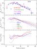 |
Fig. B.1
Top: observed surface density profiles of various SFR tracers (see text); the dotted curve – with no error bars – is the analytical form suggested by Green (2013) and it is here adopted as representative of the MW SFR profile. Middle: theoretical or empirical SF rates compared to the adopted profile of SFR tracers (the dotted curve from the upper panel); all profiles are normalised to the same value in R0 = 8 kpc. Bottom: ratio of the theoretical or empirical profiles to the adopted observed one. |
| Open with DEXTER | |
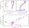 |
Fig. B.2
Top: SFR surface density vs. total gas surface density (left) and vs. H2 (right) for the MW disk, in the region between 2 and 13 kpc. In both panels, curves represent the same quantities as in Fig. B.1; the long dashed curve (SFR ∝ Σ(H2)) corresponds quantitatively to the fit of Bigiel et al. (2008) to extragalactic data and fits the adopted “observed” SFR profile in the MW disk quite well. Bottom: the “observed” SFR vs. gas relation in the MW is compared to a compilation of extragalactic data from Krumholz et al. (2012). |
| Open with DEXTER | |
There is reasonably good agreement between all the SFR tracers of Fig. B.1, with the exception of the one for luminous massive stars of the RMS survey (Urquhart et al. 2014), which differs considerably from the others inside 4 kpc (where selection biases are expected to be more important, even for such luminous stars) and displays an unexpected enhancement in the region around 9 kpc. Baring those differences, we adopt Eq. (B.1) as the expression for the radial dependence of the SFR in the MW disk, after normalising it (by putting A = 3.5M⊙/kpc2/y) to the total SFR rate of the Milky Way ΨMW = 2M⊙/y (Chomiuk & Povich 2011): 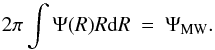 (B.2)In the middle panel of Fig. B.1, we compare the “observed” SFR profile with various theoretical or empirical profiles in the literature, which make use of the corresponding profiles of total or molecular gas discussed in this section. All of them are normalised to the adopted observed value of the SFR in the solar neighbourhood.
The most widely used SFR prescription is the so-called “Schmidt-Kennicut” law, based on observations of quiescent and active disk galaxies: ![]() , where the gas surface density ΣG runs over three orders of magnitude and the data suggest k = 1.5. It turns out that this form of the SFR, with k = 1.5 is too flat to fit the MW data: Misiriotis et al. (2006) find k = 2 from their modelling of the IR emission of the MW. Also, it is well known that a steeper function is required in galactic chemical evolution models to explain the observed abundance gradients in the MW disk.
, where the gas surface density ΣG runs over three orders of magnitude and the data suggest k = 1.5. It turns out that this form of the SFR, with k = 1.5 is too flat to fit the MW data: Misiriotis et al. (2006) find k = 2 from their modelling of the IR emission of the MW. Also, it is well known that a steeper function is required in galactic chemical evolution models to explain the observed abundance gradients in the MW disk.
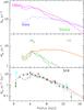 |
Fig. B.3
Top: observed molecular fraction |
| Open with DEXTER | |
Boissier & Prantzos (1999) adopted a law of the form ![]() ; the factor V(R) /R is ∝ 1 /R for a flat curve of the rotational velocity V(R) and is attributed to spiral waves inducing star formation with that frequency (Wyse 1986; Wyse & Silk 1989). On the other hand, models by Chiappini (2001) adopt
; the factor V(R) /R is ∝ 1 /R for a flat curve of the rotational velocity V(R) and is attributed to spiral waves inducing star formation with that frequency (Wyse 1986; Wyse & Silk 1989). On the other hand, models by Chiappini (2001) adopt ![]() , where ΣTOT is the total disk surface density (dominated in the inner Galaxy by the rapidly increasing stellar profile), and they introduced a cut-off in the SFR efficiency, below 2 M⊙/pc2. Both SFR laws also appear in the middle and lower panels of Fig. B.1: they fit relatively well the “observed” SFR profile and it turns out that the corresponding models reproduce several key properties of the MW disk relatively well.
, where ΣTOT is the total disk surface density (dominated in the inner Galaxy by the rapidly increasing stellar profile), and they introduced a cut-off in the SFR efficiency, below 2 M⊙/pc2. Both SFR laws also appear in the middle and lower panels of Fig. B.1: they fit relatively well the “observed” SFR profile and it turns out that the corresponding models reproduce several key properties of the MW disk relatively well.
The aforementioned laws make use of the total gaseous profile of the disk. Based on a detailed, sub-kpc scale, observations of a large sample of disk galaxies, Bigiel et al. (2008) have found that the SFR appears to follow the H2 surface density, rather than the HI or the total gas surface density. In a companion paper, Leroy et al. (2008) argue that the observed radial decline in star formation efficiency is too steep to be reproduced only by increases in the free-fall time or orbital time and they find no clear indications of a cut-off in the SFR.
Following these studies, we checked whether such a correspondence between the adopted SFR and molecular gas profiles also holds in the MW disk. The comparison, presented in the middle and lower panels of Fig. B.1, is favourable to that idea: the SFR follows the H2 profile to better than 30% in the 3−13 kpc range.
Figure B.2 displays the data in a different way, with SFR surface density vs. gas (total or molecular) surface densities. In the top left panel, it appears that the “observed” SFR varies too steeply with the total gas density and it cannot be fit with a simple Schmidt-Kennicutt" law ![]() ; a strong radial dependence of the SF efficiency, such as the aforementioned ones, is required to improve the situation. In the top right panel it is seen that the “observed” SFR increases almost linearly with H2, and that the SFR proposed by Bigiel et al. (2008), Ψ = 0.009ΣH2/(10 M⊙/pc2), reproduces the data quite well. The measurement of Bigiel et al. (2008) concern H2 surface densities above 3 M⊙/pc2, i.e. they correspond to the upper half of the figure. It appears that, at least in the case of the MW, that dependence is prolonged to even smaller surface densities. In the bottom panel of Fig. B.2 the “observed” SFR vs. gas relation in the MW disk is compared to data of a sample of disk galaxies from Krumholz et al. (2012). It is clearly seen that the MW disk SFR corresponds to a narrow range of gas surface densities, so the extragalactic data of SFR vs. gas cannot be used as guide to the MW SFR; in contrast, data on MW SFR vs. H2 cover a wider dynamical range of H2 and offer convincing evidence of a linear relationship between the two quantities.
; a strong radial dependence of the SF efficiency, such as the aforementioned ones, is required to improve the situation. In the top right panel it is seen that the “observed” SFR increases almost linearly with H2, and that the SFR proposed by Bigiel et al. (2008), Ψ = 0.009ΣH2/(10 M⊙/pc2), reproduces the data quite well. The measurement of Bigiel et al. (2008) concern H2 surface densities above 3 M⊙/pc2, i.e. they correspond to the upper half of the figure. It appears that, at least in the case of the MW, that dependence is prolonged to even smaller surface densities. In the bottom panel of Fig. B.2 the “observed” SFR vs. gas relation in the MW disk is compared to data of a sample of disk galaxies from Krumholz et al. (2012). It is clearly seen that the MW disk SFR corresponds to a narrow range of gas surface densities, so the extragalactic data of SFR vs. gas cannot be used as guide to the MW SFR; in contrast, data on MW SFR vs. H2 cover a wider dynamical range of H2 and offer convincing evidence of a linear relationship between the two quantities.
In view of this observational support, both for the MW disk (this work) and for external galaxies (Bigiel et al. 2008; Leroy et al. 2008), we adopt here a star formation law depending on the H2 surface density. In order to calculate it in the model of chemical evolution we adopt the semi-emi-empirical prescription of Blitz & Rosolowsky (2006) for the ratio Rmol = H2/HI and we find rather good agreement between the observed and theoretically calculated molecular fractions in the MW disk 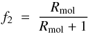 (B.3)as seen in the top panel of Fig. B.3. The resulting radial profiles H2(R) = f2(R) ΣG(R) and HI(R) = [ 1−f2(R) ] ΣG(R) also compare favourably to the observed ones (middle panel). Finally, the corresponding SFR (Eq. (3) in Bigiel et al. 2008, but with a coefficient 0.0016 instead of 0.008)
 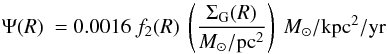 (B.4)reproduces well the “observed” SFR profile of the MW disk in the 4−12 kpc region, and somewhat less successfully outside that region (bottom panel). This agreement has already found in Blitz & Rosolowsky (2006), but with older data for the gas and SFR profiles of the MW.
Appendix C: Chemical evolution
In studies of galactic chemical evolution, the changes in the chemical composition of the system are described by a system of integro-differential equations. The mass of element/isotope i in the gas is mi = mGXi, (where mG is the mass of the gas and Xi is the mass fraction of i) and its evolution is given by: ![]() (C.1)i.e. star formation at a rate Ψ removes element i from the ISM at a rate ΨXi, while at the same time stars inject in the ISM that element at a rate Ei(t). The rate of ejection of element i by stars is given by:
(C.1)i.e. star formation at a rate Ψ removes element i from the ISM at a rate ΨXi, while at the same time stars inject in the ISM that element at a rate Ei(t). The rate of ejection of element i by stars is given by: 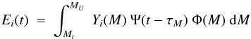 (C.2)where the star of mass M, created at the time t − τM, dies at time t (if its lifetime τM is lower than t) and releases a mass Yi(M) in the form of element/isotope i (stellar yield of i from mass M). Here, Φ(M) = dN/ dM is the IMF, assumed to be independent of time t, Mt is the mass of the smallest star that has lifetime τM = t and MU is the most massive star of the IMF.
 |
Fig. C.1
Top: stellar mass vs. lifetime. Middle: stellar death rate after an initial “burst” forming 1 M⊙ of stars: dN/ dt = dN/ dM × dM/ dt, where dN/ dM is the stellar IMF and dM/ dt the derivative of the curve in the top panel. The thick portion of the curve (up to ~35 My, corresponding to a star of 8 M⊙) is the rate of CCSN. The bottom right part of the middle panel displays the corresponding SNIa rate (the time delay distribution or TDD) adopted in this work (thick curve); it is a mixture of the Greggio (2005) formulation for the SD scenario up to 4.5 Gyr and an extrapolation ∝ t-1 after that time, in order to fit the data points from Maoz et al. (2012; filled circles) and from Maoz et al. (2010; squares). Bottom: time-integrated numbers of CCSN (thick portion of upper curve), single stars of mass M< 8M⊙ (thin portion of upper curve) and SNIa (lower curve), as a function of time, for an initial “burst” of 1 M⊙. |
| Open with DEXTER | |
Because of the presence of the term Ψ(t − τM), Eqs. (C.1) and (C.2) have to be solved numerically (except if specific assumptions, like the instantaneous recycling approximation – IRA – are made). The integral (C.2) is evaluated over the stellar masses, properly weighted by the term Ψ(t − τM) corresponding in each mass M. It is explicitly assumed in that case that all the stellar masses created in a given place, release their ejecta in that same place.
This assumption does not hold anymore if stars are allowed to travel away from their birth places before dying. In that case, the mass Ei(t) released in a given place of spatial coordinate R and at time t is the sum of the ejecta of stars born in various places R′ and times t − t′, with different SFRs Ψ(t′,R′) for all stellar masses M with lifetimes τM<t − t′ Instead of Eq. (C.2), the isochrone formalism, concerning instantaneous “bursts” of star formation or single stellar populations (SSP), has to be used then Eq. (C.2) is rewritten as  (C.3)where dN = Φ(M)dM is the number of stars between M and M + dM and Ψ(t′)dt′ is the mass of stars (in M⊙) created in time interval dt′ at time t′. The term (dN/ dt′)t − t′ represents the stellar death rate (by number) at time t of a unit mass of stars born in an instantaneous burst at time t − t′. The term Yi(M)dN/ dt represents the corresponding rate of release of element i in M⊙/yr.
Expression (C.3) is equivalent to expression (C.2) and it is used in N-body+SPH simulations (see Lia et al. 2002 or Wiersma et al. 2009), since it allows one to account for the ejecta released in a given place by “star particles” produced with different SFRs in other places (see main text). It naturally incorporates the metallicity dependence of the stellar yields and of the stellar lifetimes, both found in the term Yi(M,Z)(dN/ dt)(Z).
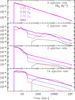 |
Fig. C.2
Ejection rates of hydrogen, carbon, oxygen and Fe from a stellar population of 1 M⊙ as a function of time. Yields are from Nomoto et al. (2013).The curves represent different metallicities, as indicated in the top panel. The dotted curves show the contribution of SNIa (resulting from a SSP of 1 M⊙) to the production of those elements. |
| Open with DEXTER | |
As in Boissier & Prantzos (1999), we use here the stellar lifetimes τ(M,Z) of Schaller et al. (1992) for stars in the mass range 0.1−120 M⊙ and for two metallicities Z⊙ and 0.05 Z⊙ (covering the metallicity of the MW disk during its whole evolution except, perhaps, its earliest phases).
We adopt the stellar IMF of Kroupa (2002) in the mass range 0.1−100 M⊙, but with a slope x = −2.7 in the range 1−100 M⊙ (the “Scalo slope”), since the “Salpeter slope” of −2.35 overproduces metals in the evolution of the solar neighbourhood. Moreover, the “Scalo” slope is similar to the one of the integrated galactic IMF (IGIMF) suggested in e.g. Kroupa (2008), which is appropriate for galactic evolution studies.
We adopt the yields provided by Nomoto et al. (2013)6. They concern both low and intermediate mass stars in the mass range 0.9 to 3.5 M⊙ (calculations from Karakas 2010)
and for massive stars in the range 11−40 M⊙. They are particularly adapted to the study of the galactic disk, because they cover a uniform grid of 6 initial metallicities (Z = 0, 0.001, 0.002, 0.004, 0.008, 0.02 and 0.05, i.e. from 0 to about 3 times solar), allowing for a detailed study of both the inner and the outer MW regions. This constitutes a clear advantage over other sets of widely used yields (e.g. Woosley & Weaver 1995). The massive star models of Nomoto et al. (2013) have mass loss but no rotation; yields of hypernovae (very energetic explosions) are also provided but we do not use them here. We include all 82 stable isotopic species from H to Ge. We calculate their evolution and we sum up at each time step to obtain the corresponding evolution of their elemental abundances. We note that the use of the yields in chemical evolution calculations requires some interpolation in the mass range of the super-AGB stars (6 or 8 to 11 M⊙).
We force the sum of the ejected masses of all isotopes of a star to be equal to the original stellar mass minus the one of the compact residue (white dwarf, neutron star or black hole). This is important in order to ensure mass conservation in the system during the evolution. We interpolate logarithmically the yields in metallicity and in the mass range between 3.5 and 11 M⊙, and we include a detailed treatment for the production of the light nuclides Li, Be and B by cosmic rays (Prantzos 2012).
For the rate of SNIa we adopt a semi-empirical approach: the observational data of recent surveys are described well by a power-law in time, of the form ∝ t-1, e.g. Maoz & Mannucci (2012) and references therein. At the earliest times, the DTD is unknown/uncertain, but a cut-off must certainly exist before the formation of the first white dwarfs (~35−40 Myr after the birth of the SSP). We adopt then the formulation of Greggio (2005) for the single-degenerate (SD) scenario of SNIa. That formulation reproduces, in fact, the observations up to ~4−5 Gyr (see Fig. C.1, middle panel) quite well. For longer timescales, where the SD scenario fails, we simply adopt the t-1 power law. The corresponding SNIa rate at time t from all previous SSP is obtained as  (C.4)As in GP2000 we adopt the SNIa yields of Iwamoto et al. (1999) for Z = 0 and Z = Z⊙, interpolating logarithmically in metallicity between those values.
In Fig. C.1 we show the results for a SSP concerning the stellar death rates, including the CCSN rate, the SNIa rate (middle panel) and the corresponding time-integrated rates. With the adopted IMF, there are about 4.5 × 10⁻³ CCSN and 1.2 × 10⁻³ SNIa for every M⊙ of stars formed.
In Fig. C.2 we present the ejection rates for H, C, O and Fe as a function of time, for single stars (3 initial metallicities) and for SNIa. SNIa produce more than half of solar Fe and they make minor contributions to the production of “light” metals like C or O (but substantial ones to the production of Si or Ca).
We made extensive tests of the implemented SSP formalism (Eq. (C.3)) against the “classical” one (Eq. (C.1)) and found excellent agreement in all cases.
© ESO, 2015
Current usage metrics show cumulative count of Article Views (full-text article views including HTML views, PDF and ePub downloads, according to the available data) and Abstracts Views on Vision4Press platform.
Data correspond to usage on the plateform after 2015. The current usage metrics is available 48-96 hours after online publication and is updated daily on week days.
Initial download of the metrics may take a while.