| Issue |
A&A
Volume 666, October 2022
|
|
|---|---|---|
| Article Number | A130 | |
| Number of page(s) | 20 | |
| Section | Galactic structure, stellar clusters and populations | |
| DOI | https://doi.org/10.1051/0004-6361/202243780 | |
| Published online | 17 October 2022 | |
Towards a fully consistent Milky Way disk model
V. The disk model for 4–14 kpc
Astronomisches Rechen-Institut, Zentrum für Astronomie der Universität Heidelberg, Mönchhofstr. 12–14, 69120 Heidelberg, Germany
e-mail: This email address is being protected from spambots. You need JavaScript enabled to view it.
Received:
13
April
2022
Accepted:
29
June
2022
Abstract
Context. The semi-analytic Just-Jahreiß (JJ) model of the Galactic disk is a flexible tool for stellar population synthesis with a fine age resolution of 25 Myr. The model has recently been calibrated in the solar neighbourhood against the Gaia DR2 stars. We have identified two star-formation bursts within the last ∼4 Gyr of the local star-formation rate (SFR) history.
Aims. In this work we present a generalised version of the JJ model that incorporates our findings for the solar neighbourhood and is applicable to a wide range of galactocentric distances, 4 kpc ≲R ≲ 14 kpc.
Methods. The JJ model includes the four flattened and two spheroidal components of the Milky Way, describing it as an axisymmetric system. The thin and thick disks, as well as atomic and molecular gas layers, are assumed to have exponential radial surface density profiles. Spherical stellar halo and dark matter in the form of a cored isothermal sphere are also added to the model. The overall thickness of the thin disk is assumed to be constant at all radii, though model realisations with a flaring disk can also be tested. The adopted radial variation in the thin-disk SFR reflects the inside-out disk growth scenario. Motivated by our findings for the solar neighbourhood, we allow a smooth power-law SFR continuum to be modified by an arbitrary number of Gaussian peaks. Additionally, the vertical kinematics of the stellar populations associated with these episodes of star-formation excess is allowed to differ from the kinematics prescribed by the age-velocity dispersion relation for the thin-disk populations of the same age.
Results. We present a public code of the JJ model complemented by the three sets of isochrones generated by the stellar tracks and isochrones with the PAdova and TRieste Stellar Evolution Code (PARSEC), the Modules and Experiments in Stellar Astrophysics (MESA) Isochrones and Stellar Tracks (MIST), and a Bag of Stellar Tracks and Isochrones (BaSTI). Assuming a plausible set of parameters, we take the first step towards calibrating the JJ model at non-solar radii. Using metallicity distributions of the red clump giants from the Apache Point Observatory Galactic Evolution Experiment (APOGEE), we constrain the radial variation of the JJ-model age-metallicity relation and propose a new analytic form for the age-metallicity relation function.
Conclusions. The generalised JJ model is a publicly available tool for studying different stellar populations across the Milky Way disk. With its fine age resolution and flexibility, it can be particularly useful for reconstructing the thin-disk SFR, as a variety of different SFR shapes can be constructed within its framework.
Key words: Galaxy: disk / Galaxy: kinematics and dynamics / solar neighborhood / Galaxy: evolution
© K. Sysoliatina and A. Just 2022
 Open Access article, published by EDP Sciences, under the terms of the Creative Commons Attribution License (https://creativecommons.org/licenses/by/4.0), which permits unrestricted use, distribution, and reproduction in any medium, provided the original work is properly cited.
This article is published in open access under the Subscribe-to-Open model. This email address is being protected from spambots. You need JavaScript enabled to view it. to support open access publication.
1. Introduction
During the last few decades, extensive astrometric, photometric, and spectroscopic data on the Milky Way (MW) stellar populations have been collected. As a result, it became possible to build complex and realistic MW models and constrain their parameters by comparing their predictions to the observed stellar distributions, motions, chemical abundances, and ages. And though no exhaustive MW model exists at the moment, significant progress has been achieved towards understanding the MW evolutionary processes.
Relatively simple semi-analytic MW models, such as the TRI-dimensional modeL of thE GALaxy (TRILEGAL1), a priori prescribe some observationally motivated spatial density distributions for the Galactic components. With the help of a stellar evolution library and additional assumptions about the MW2 star-formation rate (SFR) history, initial mass function (IMF), and age-metallicity relation (AMR), these densities are then transformed into star counts within some observational field (Girardi et al. 2005; Girardi 2016). Even with this simple approach it is possible to obtain realistic star count predictions for the volumes where the model has been trained; as a result, the optimised model parameters can tell us a lot about the evolution of the MW stellar components (Pieres et al. 2020; Dal Tio et al. 2021).
List of abbreviations used in this paper.
One of the most comprehensive semi-analytic MW models to date is the Besançon Galaxy model (BGM3; Robin et al. 2003, 2012, 2017; Czekaj et al. 2014; Bienaymé et al. 2018). This dynamically self-consistent model describes gaseous, stellar, and dark matter (DM) MW content in terms of sets of sub-components characterised by the different kinematics, chemistry, ages, and densities. The BGM also includes non-axisymmetric features, such as the bar, spiral arms, disk flare, and warp (Amôres et al. 2017), and accounts for extinction. The model has many applications in the field of Galactic studies – for example, Mor et al. (2019) optimised its predictions using the second data release (DR2) of the Gaia mission (Gaia Collaboration 2016, 2018) and find evidence of an increase in star-formation (SF) activity in the last ∼2–3 Gyr of the MW disk history. However, the results of that work do not allow the authors to draw a firm conclusion about the SFR shape because of the limited age resolution of the model: there are only seven sub-populations representing the thin disk in the BGM, and this may be not enough to decipher with certainty the evolutionary complexity of the MW disk.
During the last decade, we have been developing a semi-analytic model of the MW disk with a time resolution as fine as 25 Myr (Just & Jahreiß 2010, hereafter Paper I). So rather than having seven sub-populations as in the BGM, the Just-Jahreiß (JJ) model builds the thin disk from 520 mono-age sub-populations. This allows the disk structure and evolution to be studied in great detail, which also allows theoretical modelling to keep up with the ever-growing amount and quality of data accumulated for the MW stellar populations.
The JJ model is based on an iterative solving of the Poisson equation, and thus reconstructs a self-consistent pair of the overall vertical gravitational potential and density profile. The thin disk is modelled in the presence of gas, thick disk, stellar halo, and DM components. The disk evolution is governed by four input functions: the SFR, IMF, age-velocity dispersion relation (AVR), and AMR. So far, the JJ model has been tested many times and calibrated against different data in the solar neighbourhood. In Just et al. (2011, hereafter Paper II) we used star counts towards the north Galactic pole from the seventh data release (DR7) of the Sloan Digital Sky Survey (SDSS; Abazajian et al. 2009) to optimise the SFR and thick-disk parameters. Rybizki & Just (2015, hereafter Paper III) improved the IMF with the help of data provided by the HIgh Precision PARallax COllecting Satellite (HIPPARCOS; van Leeuwen 2007) complemented by an updated version of the Catalogue of Nearby Stars (CNS 4; Jahreiß et al. 1997). In Sysoliatina et al. (2018) we demonstrated a good model-to-data consistency (with a ∼7.3-% discrepancy in terms of star counts) in the local 1-kpc height cylinder using stars from the Radial Velocity Experiment survey (RAVE; Steinmetz et al. 2006; Kunder et al. 2017) and the Tycho-Gaia Astrometric Solution catalogue (TGAS; Michalik et al. 2015; Lindegren et al. 2016). Most recently, we used Gaia DR2 stars within 600 pc of the Sun and simultaneously optimised 22 model parameters within the Bayesian framework (Sysoliatina & Just 2021, hereafter Paper IV). We also calibrated the AMR against the local red clump (RC) sample from the Apache Point Observatory Galactic Evolution Experiment survey (APOGEE; Eisenstein et al. 2011; Bovy et al. 2014; Majewski et al. 2017). We have identified two recent SF burst episodes in the thin-disk evolutionary history, which happened ∼0.5 Gyr and ∼3 Gyr ago and left behind dynamically heated fossil populations.
In this paper we generalise our local JJ model for the range of galactocentric distances 4 kpc ≲R≲ 14 kpc by building the disk out of a set of independent radial annuli. We assume radially exponential gaseous, thin and thick disks, a spherical stellar halo, and a cored isothermal DM halo. We fix the disk thickness by assuming a constant-thickness thick disk and a constant-thickness or flaring thin disk and allow radial variations in the input functions SFR, AVR, and AMR, which correspond to the inside-out disk growth scenario. We present a publicly available tool, python package jjmodel, which can be used to perform stellar population synthesis within the JJ-model framework. Following Paper IV, we constrain the thin- and thick-disk AMR using the generalised JJ model with the radially extended APOGEE RC sample. We then propose a new analytic form for the thin-disk AMR, which is able to comprise the variation in its shape across the studied distances, 4 kpc < R < 14 kpc. Thus, we add another dimension to the fine JJ-model resolution: the numerous MW mono-age sub-populations can be now synthesised over a fine R-z grid.
This paper has the following structure. In Sect. 2 we review the JJ-model components, explain how different ingredients of the local JJ model are now extended to other galactocentric distances, and summarise the overall scheme of mock sample modelling. Section 3 contains a description of a test model and its predictions for the MW disk properties. In Sect. 4 we reconstruct the radially dependent AMR using APOGEE RC data. Then, we discuss the obtained results for AMR, as well as the generalised JJ-model predictions and their possible applications, in Sect. 5. Finally, we summarise the main aspects of this work in Sect. 6.
2. Generalised JJ model
In this section we introduce our key assumptions about the structure and properties of the Galaxy (Sect. 2.1), recall stellar dynamic equations used for calculation of the Galactic potential (Sect. 2.2), and review our treatment of the MW components in the local JJ model to generalise it for the whole MW disk (Sects. 2.3–2.8). We also briefly remind our approach to converting the modelled densities into mock samples (Sect. 2.9) and present an overall scheme of building the MW disk within the JJ-model framework (Sect. 2.10).
2.1. Basic assumptions and limitations
Before going into details, we briefly summarise the main assumptions on which the JJ model is based. We also mention limitations imposed by these assumptions on the model applicability (more in Sect. 2.2).
First, the MW disk rests in a steady state. This statement is in harmony with the observational data, which show no evidence of fast evolutionary processes happening in our Galaxy at the present day (no major merger, no activity in the nucleus). All transformations of the MW populations’ distribution functions occur slowly, as a result of collective interactions of the MW components (the so-called secular evolution). Thus, for our purpose of describing the MW at the present-day time snapshot, it is safe to treat the system as a steady one.
Second, the MW disk is axisymmetric and plane-symmetric (no bar, spiral arms, or warp are included). This implies that the JJ model cannot be used at small radii, R ≲ 4 kpc, where this assumption breaks because of a presence of the bar. Also, for comparison to the data, unless the model is used to reveal the underlying deviations from the smooth density distribution, the JJ-model predictions need to be averaged over large enough volumes to smear out small-scale density perturbations, such as overdensities in the spiral arms. Due to the absence of the warp, the predicted vertical structure can be reliable up to moderate radii, R ≲ 14 kpc.
Third, the system is flattened (radial and vertical dynamics can be decoupled). Within the range of considered galactocentric distances, 4 kpc < R < 14 kpc, this holds up to |z|≈2 kpc (see Sect. 2.2 for details).
Fourth, the MW stellar, gaseous, and DM components are represented by an individual or multiple isothermal sub-populations. Some of these sub-populations are assumed to be globally isothermal (stellar and DM halo), while others are isothermal only locally at fixed R (thin disk, thick disk, molecular and atomic gas).
Fifth, all sub-populations are in equilibrium with the total gravitational potential (Poisson and Jeans equations can be applied). This may not hold for very young populations, which did not have enough time to reach the equilibrium. Thus, the model cannot be applied to the youngest populations (O- and B-type stars).
2.2. Vertical profiles
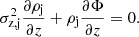
At each galactocentric distance, the overall density in the JJ model is prescribed as a sum of i different MW components: stellar (thin disk, thick disk, stellar halo), gaseous (molecular and atomic gas), and DM4:
 (1)
(1)
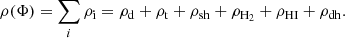
Here Φ is the total gravitational potential produced by this matter. For a single isothermal sub-population with the vertical velocity dispersion σz, j, its density is linked to the total gravitational potential according to the Jeans equation:
 (2)
(2)
Here we dropped a time-derivative term assuming a steady state. We also ignored two cross-terms containing σRz, essentially implying that the radial and vertical motions in the Galactic disk are decoupled. It can be shown that the ratio of these cross-terms to the rest of the terms in the Jeans equation is of the order of z/R ⋅ hj/Rj, where hj and Rj are the sub-population’s scale height and scale length, respectively (Bahcall 1984; Bienayme et al. 1987). In a flattened MW-like system, hj ≪ Rj, and therefore, within the range of radii 4 kpc < R < 14 kpc this ratio is small up to |z|≈2 kpc.
The solution of Eq. (2) implies that the vertical density fall-off of the isothermal sub-population is an exponential function of the total gravitational potential:
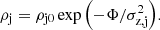 (3)
(3)
Here potential is zero in the Galactic plane, and ρj0 is the sub-population’s midplane density defined via its surface density Σj and scale height hj:
 (4)
(4)
As a next step, we assume that all MW components in Eq. (1) can be represented by a single or multiple mono-age isothermal sub-populations, whose vertical density profiles follow Eq. (3). As a result, Eq. (1) can be turned into a specific function of the total potential with the vertical velocity dispersions and midplane densities of sub-populations as model parameters. Then, we can substitute this function into the Poisson equation and find a self-consistent potential-density pair.
For an axisymmetric system, the Poisson equation in cylindrical coordinates can be written as
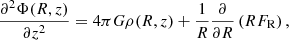 (5)
(5)
where G is the gravitational constant and FR = −∂Φ(R, z)/∂R is the radial force. It is common to assume that in flattened systems the second term on the right-hand side (the radial term) is not important in comparison to the first one (the density term), and thus, can be neglected (Binney & Tremaine 2008). Indeed, as a zero-order approximation, RFR can be replaced by its value in the plane, namely, by the squared circular velocity  . As the MW rotation curve is nearly flat in a wide range of galactocentric distances, the radial term is vanishingly small and can be dropped. For the rotation curve reconstruction in Sysoliatina et al. (2018), we developed a more accurate treatment of the radial force that also includes dependence on z (see Eq. (4.19) in Sysoliatina 2018). Thus, we can estimate a ratio of the radial to density terms, in the framework of our MW mass model used in Sysoliatina et al. (2018). We find that in the range of galactocentric distances 4 kpc < R< 14 kpc, this ratio is ∼0.01 in the Galactic plane and may become important only at |z|≈2 kpc in the inner disk, R ≲ 5 kpc, where it reaches ∼0.2–0.5. But even in this case, the radial term can still be neglected as it remains smaller than the density term uncertainty. The latter is dominated by the uncertainty of a poorly known DM density, which typically reaches tens of percent (Read 2014).
With these considerations taken into account, we neglect the radial term in Eq. (5) that significantly simplifies our problem. The Poisson equation without the radial term states that the vertical gravitational potential at some radius is produced only by matter at this radius, that is to say, the radial and vertical structure of the disk can be treated separately. This means that our approach of building the MW disk out of a set of independent radial annuli is justified. At each radius, the solution of the simplified Poisson equation reads as
 (6)
(6)
Here ρ(Φ) is the total density at this radius given by Eq. (1) with substitution from Eqs. (3) and (4).
In the following subsections, we describe in detail how each MW component is modelled over the considered range of galactocentric radii.
2.3. Thin disk
There are four analytic functions in the JJ model, which reflect main aspects of the MW thin-disk evolution and describe its present-day state: IMF, SFR, AVR, and AMR. The thin disk has a present-day age of tp = 13 Gyr and consists of a set of locally isothermal sub-populations covering the whole age range with a fine resolution of tr = 25 Myr. This results into 520 thin-disk sub-populations, each characterised by its present-day mean age, metallicity, vertical velocity dispersion, and surface density. Below we explain how each of these quantities are prescribed (Sects. 2.3.1–2.3.4), and how, together with the thick-disk and halo sub-populations, they are eventually converted into star counts (Sect. 2.9).
2.3.1. IMF
For the IMF, we adopt a four-slope broken power law. Its up-to-date parameters are listed in Paper IV (Table 4 and Sect. 4.6.2) where we optimised them in consistency with the kinematic and SFR parameters using the local Gaia DR2 sample. This default JJ-model IMF is also applied during stellar population synthesis of the thick disk and halo (Sect. 2.9). In the jjmodel package, the user can both change the IMF parameters and customise the model by defining another IMF law.
It is worth mentioning here that there is different observational evidence indicating that IMF is more top-heavy in the environments with low metallicity and high density (Bartko et al. 2010; Banerjee & Kroupa 2012; Kalari et al. 2018), and thus, also in the early Universe. On the other side, massive early-type galaxies seem to have a bottom-heavy IMF, and the same is reported for the MW low-metallicity stars in Hallakoun & Maoz (2021). A possibility for IMF varying in space and time is discussed in the literature (Kroupa et al. 2020) and tested with various methods – for example, in the cosmological simulations of the MW-like galaxies (Guszejnov et al. 2017) or with semi-analytic models of SF in pre-stellar cores of different metallicities (Tanaka et al. 2017, 2018, 2019). However, most of the observed IMF variations are moderate and can be fitted into the universal IMF paradigm (Bastian et al. 2010; Offner et al. 2014). In our model we chose to stick to the conventional universal IMF for all disk sub-populations at all R and z. We do this for two reasons: (1) spatially and time-dependent IMF remains debatable, and (2) the regions we model have never belonged to the environments with extreme physical conditions, such as the Galactic centre, where the most significant deviations of the canonical IMF are observed.
2.3.2. AMR
The AMR function describes in a simple way the chemical evolution of the disk by linking the metallicity and age of its stellar sub-populations. In the previous JJ-model versions, we used for the thin-disk AMR a four-parameter logarithmic law (Eqs. (21) and (22) in Paper IV). It describes a relatively quick chemical enrichment during the first ∼0.5–1 Gyr of the disk evolution with a subsequent quasi-linear increase of metallicity with age in the solar neighbourhood.
There are two options for introducing the thin-disk AMR in the jjmodel code. More sophisticated and default AMR is described by a seven-parameter tanh-law, whose parameters are constants, linear or broken linear laws of R (Sect. 4.2.4). By construction, this AMR is consistent with the observed metallicity distribution (MD) of the APOGEE RC stars across the disk, the reconstruction process of this AMR is described in Sect. 4.
The second and simpler way to prescribe the thin-disk AMR is analogous to how we extend the local thin-disk SFR to other radii (Sect. 2.3.3): parameters of the four-parameter logarithmic AMR function with known values at R⊙ (Table 3 in Paper IV) are assumed to vary with radius according to power laws with predefined slopes.
2.3.3. SFR
Starting from Paper I, the default thin-disk SFR was a power-law function with a peak at ∼10 Gyr ago and a monotonous decline to the present day. In Paper IV, we found that the thin-disk SFR prescribed in such a way is inconsistent with the observed Gaia DR2 star counts of young populations in the local volume. The data-to-model consistency can be significantly improved by adding to the declining SFR continuum two Gaussian peaks centred at ages of ∼0.5 Gyr and ∼3 Gyr. This result is consistent with Mor et al. (2019) who find a single SF burst centred at the age of 2–3 Gyr. Also, Ruiz-Lara et al. (2020) report three SF enhancements 5.7 Gyr, 1.9 Gyr, and 1 Gyr ago, which were presumably triggered by recurrent passages of the Sagittarius dwarf galaxy. Sahlholdt et al. (2022) studied disk subgiants and dwarfs from the Third Data Release of the Galactic Archaeology with HERMES (GALAH DR3; Buder et al. 2021) and Gaia Early Data Release 3 (EDR3; Gaia Collaboration 2021). The authors have also identified several enhancements in the disk SFR with the most recent SF peak at ages 2–4 Gyr, in agreement with the above mentioned studies. Motivated by these findings, we now define the thin-disk SFR as a standard smooth continuum that can be modified by an arbitrary number of overlaying Gaussian peaks, which allows the construction and testing of SFR functions of complicated shapes.
At a fixed radius, we define the thin-disk SFR as follows:
 (7)
(7)
It is a product of a normalisation constant and a time-dependent function; the latter consists of two terms that are related to the continuum and additional peaks (denoted by ‘dc’ and ‘dp’, respectively). The function is normalised to the overall present-day thin-disk surface density Σd:
 (8)
(8)
A mass loss function gd(t) in Eq. (8) accounts for the cumulative effect of stellar evolution and is needed to convert the present-day stellar mass into the mass at the time of formation. In particular, gd(t) gives a fraction of a sub-population’s mass survived to the present day in the form of stars (including remnants). This fraction depends on the IMF and the sub-population’s metallicity (i.e., AMR; for gd(t) expression see Eq. (9) in Paper IV). We calculate these fractions with the default JJ-model IMF over the grid of metallicities and ages using the chemical evolution code Chempy5 (Rybizki et al. 2017). For each realisation of the JJ model, the mass loss function is then constructed in consistency with the chosen AMR by interpolation over the tabulated values. As the mass loss function depends on the IMF very weakly, and an impact of the mass loss function itself on the modelled quantities is of a higher order than of SFR and AVR, we do not provide a tabulated gd(t) for IMF laws other than our standard four-slope broken power law.
The continuum part of the thin-disk SFR is given by Eq. (10) in Paper IV, and for the sake of completeness we also reproduce it here:
 (9)
(9)
In this equation, parameters td1, td2, ζ, and η define the function’s peak position and amplitude, as well as the steepness of the declining part. Following Paper IV, we define each extra SFR peak as a Gaussian weighted by the value of the SFR continuum at the peak’s mean age and normalised to the continuum maximum value:
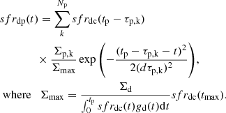 (10)
(10)
Here Σp is related to a peak’s amplitude at a given radius, and parameters τp and dτp give the mean age and the age dispersion of the peak, respectively. Galactic time tmax corresponds to the peak of the SFR continuum Σmax (Eq. (11) in Paper IV6). The summation is performed over all Np peaks. We note that this process of adding extra peaks to the SFR does not result in an increase of the overall present-day thin-disk surface density in the model. Instead, the SFR is re-normalised, such that the total surface density still equals to Σd.
We can also introduce quantities fk and f0 defined as contributions of each extra SFR peak and the continuum part to the total SFR of a sub-population:
 (11)
(11)
Here sfrdp, k(t) corresponds to the kth term of Eq. (10). These fractions are later linked to the disk kinematics (Sect. 2.3.4).
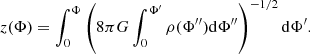
To introduce the radial variation of SFR, we allow some of its parameters to be functions of R. For the radial surface density profile, we assume an exponential law with a scale length Rd laying in the range of ∼2.5–3 kpc (Fig. 1):
 (12)
(12)
 |
Fig. 1. Radial density profiles of the JJ-model components. The dashed grey line marks the solar position. |
where Σd⊙ = Σd(R⊙) is the local surface density of the thin disk7.
Parameter td1 is a time delay of SF and can be used to construct the model with non-overlapping in time thin- and thick-disk phases. Currently, we set this parameter to zero at all radii, this corresponds to the in-parallel formation of the thin and thick disk. Parameters td2, ζ, and η are now calibrated only at the solar radius R⊙. As a first guess, we assumed for them a power-law radial dependence – a simple assumption that at the same time allows the inside-out disk growth to be mimicked.
We also assume that the thin-disk sub-populations corresponding to each of Np peaks form an overdensity normally distributed around some mean radii Rp with dispersions dRp. Then, at an arbitrary radius, the amplitude parameter of the kth SFR peak can be calculated as
 (13)
(13)
where Σp⊙ is the local value of the parameter.
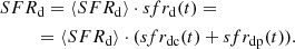
An example of the radially dependent SFR of the thin disk with two additional peaks is shown at the top panel of Fig. 2 (see also Sect. 3.1).
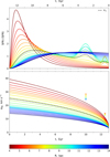 |
Fig. 2. Thin-disk SFR (top) and AVR (bottom) as functions of radius. Dashed black curves correspond to the solar neighbourhood. Crosses give the vertical velocity dispersion corresponding to the fractions of sub-populations associated with the extra SFR peaks. For the details of this model realisation, see Sect. 3.1. |
2.3.4. AVR
The vertical kinematics of the thin-disk sub-populations is represented by a power-law AVR (Eq. (30) in Paper I). At a fixed radius, we prescribe it as a product of a normalisation constant, scaling parameter σe, and an age-dependent function, such that σW(τ)=σe ⋅ avr(τ). We also link the present-day thin-disk velocity dispersion to kinematics of the molecular gas (Eq. (14) in Paper IV).
Following Paper IV, we allow some of the thin-disk sub-populations to have kinematics different from the one prescribed by the AVR. More precisely, fk fractions of sub-populations associated with the kth SFR peak (Eq. (11)) can have the vertical velocity dispersion σp, k higher than the one prescribed by the AVR function for their age. The remaining f0 fractions of the thin-disk sub-populations follow the AVR law.
To add the radial dependence, we allow one AVR parameter, its scaling factor σe, to vary with R. Thus, the AVR shape is constant at all radii and is the same as in the solar neighbourhood. The value of σe(R) is iteratively adapted at each radius to obtain the thin disk of a prescribed thickness (Sect. 2.10). By default, the thin-disk thickness is constant at all radii, which is consistent with observations of edge-on galaxies (van der Kruit & Searle 1981; Bizyaev & Mitronova 2002). However, a flaring thin disk can be also tested with the jjmodel code, for that a simple exponential flaring model from Kalberla et al. (2014) is included. In this case, the thin-disk half-thickness is described by two parameters: radius at which the flaring starts, Rf, and the flaring scale length Rdf.
If the thin-disk SFR is modelled with additional peaks and the peaks-related sub-populations are allowed to have special vertical kinematics, then at an arbitrary radius, velocity dispersion corresponding to the kth SFR peak is calculated as follows:
![Mathematical equation: $$ \begin{aligned}&\sigma _\mathrm{p,k} (R) = \sqrt{\sigma _\mathrm{ex,k} ^2 + \sigma _\mathrm{W} (R,\tau _\mathrm{p,k} )^2},\\[4pt]&\text{ where} \quad \sigma _\mathrm{ex,k} ^2 = \sigma _\mathrm p\odot ,k ^2 - \sigma _\mathrm{W} (R_\odot ,\tau _\mathrm{p,k} )^2.\nonumber \end{aligned} $$](/articles/aa/full_html/2022/10/aa43780-22/aa43780-22-eq15.gif) (14)
(14)
Here σp ⊙ ,k is the local value of the parameter, and σex, k represents the local velocity dispersion excess with respect to the AVR. The value of this excess is then quadratically added to the AVR velocity dispersion at each radius.
The bottom panel of Fig. 2 shows AVR corresponding to the JJ model with the thin disk of a constant thickness and SFR from the upper panel (Sect. 3.1). Crosses mark velocity dispersion of the SFR peaks’ populations.
2.4. Thick disk
The thick disk is modelled in the full analogy to the thin disk, but is described by a smaller number of parameters.
In the JJ model, the thick disk is constructed out of a set of mono-age locally isothermal sub-populations covering the first several Gyr of the MW evolution. The thick-disk SFR is a power-exponential function that peaks at old ages, ∼12.5 Gyr ago (Eqs. (7) and (8) and Table 2 in Paper IV). Following Paper IV, we adopt here tt2 = 4 Gyr for the duration of the thick-disk formation, which corresponds to Nt = 160 mono-age sub-populations. At a fixed radius, all thick-disk sub-populations have the same vertical velocity dispersion σt, such that kinematically the thick disk behaves as a single isothermal sub-population with the total surface density Σt. The thick disk is also characterised by its own AMR function in a form of tanh-law (Eqs. (22) and (24) in Sect. 4.2.4).
When modelling the thick disk at the different radii, we do not vary the shape of its SFR, but only normalise it to the corresponding surface density Σt(R). For the radial profile of the thick-disk surface density we assume, by analogy to Eq. (12), an exponential decline with a scale length shorter than that of the thin disk, Rt ≈ 2 kpc. The thick disk is prescribed to have a constant thickness, which we use as a constraint to calculate its velocity dispersion σt(R) at the radii other than solar. The thick-disk AMR is also not varied with galactocentric distance in our model, which is consistent with the well-mixed thick-disk population observed in our Galaxy (e.g., Hayden et al. 2015, 2020).
When the JJ model is used to model volumes extending to heights larger than zmax = 2 kpc (e.g., a cone perpendicular to the Galactic plane in Paper II and Paper IV), we extrapolate the derived thick-disk vertical profile with a sechα-law of a single isothermal sub-population. As we showed in Paper II, a simple sechα-law is still well-suited for the fitting of the thick-disk vertical profile calculated in the presence of DM and other stellar components.
2.5. Gas
Our current gas model for the solar neighbourhood is described in Paper IV, which we now extend to other galactocentric distances.
We consider two gas populations: a cold molecular (H2) and a warm atomic (HI) component. The adopted local surface densities of the molecular and atomic gas are taken from McKee et al. (2015) and are ΣH2 = 1.7 M⊙ pc−2 and ΣHI = 10.9 M⊙ pc−2, respectively (Table 2 and Table 2 in Paper IV). For the surface density radial profiles of both gas components, we assume exponential laws. Kramer & Randall (2016) discuss the radial column and surface density profiles of the atomic and molecular gas as derived by different authors before 2006–2008 yr. An averaged surface density profile of the molecular gas peaks at ∼4 kpc and then declines with a short scale length of ∼2–3 kpc. We now adopt RH2 = 3 kpc as a default value of the molecular gas scale length in the generalised JJ model. In the case of atomic gas, its surface density remains roughly constant in the wide distance range of 4–14 kpc and declines with a scale length of ∼4.5 kpc in the outer disk. Similarly, Kalberla & Dedes (2008) describe HI radial distribution: it is approximately constant in the inner disk and exponentially declining in the outer disk with a scale length of ∼3.75 kpc at 12.5 kpc < R< 30 kpc. We input RHI = 10 kpc to describe this slow decline of the atomic gas surface density with radius, which is broadly consistent with the mentioned observational data.
By analogy to the thin-disk mono-age populations, both gas components are treated as isothermal at each radius. Their vertical velocity dispersions are adapted to reproduce the prescribed scale heights of the cold and warm gas. We adopt the exponentially growing radial profiles of the H2 and HI half-thickness from Nakanishi & Sofue (2016), which the authors measured using their three-dimensional gas maps constructed on the basis of HI and CO surveys data and kinematic distances to gas clouds.
In order to get a realistic enclosed mass of gas for the MW rotation curve, we add inner holes for both gas layers at R0, H2 and R0, HI, which roughly reflects a sharp decrease of gas density in the inner disk.
2.6. Stellar halo
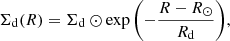
Stellar halo is modelled as a globally isothermal population of a single age tp. At each radius, its vertical density profile depends on two parameters, a universal vertical velocity dispersion σsh and its surface density at this radius Σsh(R). To get the radial surface density profile of the halo, we numerically integrate its power-law matter density profile up to zmax. The default power-law slope is αin = −2.5 corresponding to the inner halo (Bland-Hawthorn & Gerhard 2016):
 (15)
(15)
Here Σsh⊙ is the local surface density of the halo, and C is a normalisation constant, and  is a radial galactocentric coordinate.
Here we do not include halo flattening, as it will introduce only a small correction to Eq. (15). As the halo itself makes the smallest contribution to the total density among all other components, adding its flattening can be viewed as a second-order correction to the model predictions, so we neglect it for now. Though, in some cases more comprehensive modelling of the halo is justified. In Paper IV, we simulated a vertically extended sample consisting of Gaia DR2 stars selected in a cone perpendicular to the Galactic plane. To get the right halo star counts, we extended the vertical halo profile that was derived self-consistently with potential only up to zmax. For extending it to larger z, we used a broken power-law profile representing the inner and outer halo (Eq. (15) in Paper IV). If necessary, flattening can be also added at this stage.
When creating mock samples, we assume for our single-age halo a Gaussian MD with a mean [Fe/H]sh and a dispersion d[Fe/H]sh. That is to say, the halo population is further subdivided into nsh = 5–9 sub-populations with different metallicities (see also Sect. 2.9).
2.7. DM halo
The DM halo is treated in the JJ model similarly to the stellar halo. At each radius, DM component is added in the form a single isothermal population characterised by the vertical velocity dispersion σdh, which is constant at all radii, and a radially dependent surface density Σdh(R).
Assuming for the spatial DM density a cored isothermal sphere, we can express the radial DM surface density as follows:
 (16)
(16)
where Σdh⊙ is the local DM surface density, ah is the DM scaling parameter, and  . The scaling parameter is adapted to have the local total circular velocity υc, ⊙ consistent with the observed proper motion of Sgr A* (Reid et al. 2005) at the assumed solar radius R⊙, with the peculiar motion of the Sun V⊙ taken into account.
2.8. Bulge
Though we do not model the inner 4 kpc of the MW disk, the bulge presence needs to be taken into account for the calculation of the rotation curve. As we mentioned above in Sect. 2.7, we use the predicted circular velocity at the solar radius to constrain the DM scaling parameter ah, which then enters Eq. (16). For this purpose, we include the bulge in a simple form of a point mass characterised by a single parameter, mass Mb. As we do not add an inner hole in the thin- and thick-disk radial density profiles, Mb gives a difference between the bulge mass and the enclosed mass of our exponential disks extrapolated to the inner MW region.
2.9. Creating mock samples
In order to convert modelled density profiles into the mock samples of some observable populations, we need to use a stellar evolution library. As we demonstrated in Sysoliatina et al. (2018) and Paper IV, the choice of the stellar library may have a significant impact on the location of different features on the colour-magnitude diagram (CMD) and on the overall predicted star counts introducing up to ∼10-% uncertainty. To estimate the impact of the stellar library choice on our modelling, we used in our previous works different sets of isochrones that we now include in the jjmodel package.
First, our default set of isochrones is generated with the PAdova and TRieste Stellar Evolution Code (PARSEC v.1.2S; Bressan et al. 2012) and the COLIBRI code (v. S_35; Marigo et al. 2017) for the thermally pulsing asymptotic giant branch phase8. Our isochrone grid includes photometric columns in the UBVRIJHK system and GBP, GRP, and G bands for the Gaia DR2 (Maíz Apellániz & Weiler 2018) and EDR3 (Riello et al. 2021).
Second, a complementary isochrone grid is based on the MESA (Modules and Experiments in Stellar Astrophysics, Paxton et al. 2011, 2013, 2015) Isochrones and Stellar Tracks (MIST9, v.1.2; Dotter 2016; Choi et al. 2016). For this stellar library, the following photometric bands are provided in the jjmodel code: standard UBVRI, 2 Micron All Sky Survey (2MASS; Skrutskie et al. 2006) JHKs, and three GaiaG-bands for DR2 and EDR3.
Third, another complementary grid is based on the Bag of Stellar Tracks and Isochrones (BaSTI10; Hidalgo et al. 2018). The available photometric system is Gaia EDR3.
Following Paper IV, we use a wide-range metallicity grid −2.6…+0.47 of 62 isochrone tables, each covering the whole modelled age interval 0…tp with a linear step of 50 Myr. Each of the JJ-model mono-age isothermal sub-populations of the thin disk, thick disk, and stellar halo is characterised by an age-metallicity pair – according to the disks’ AMR (Sects. 2.3.2 and 2.4) and the halo MD (Sect. 2.6). In the case of the thin and thick disk sub-populations, a spread in metallicity can be additionally allowed: for each age, we assumed a Gaussian MD centred at the metallicity prescribed for this age by the AMR function, [Fe/H](τj), and characterised by dispersion d[Fe/H]dt, which is the same for all ages. In practice, this means that we increase the number of modelled age-metallicity pairs by the number of sub-populations used to sample the assumed MD at each age, ndt. Though, this added complexity slows down the calculation process, it can help to mimic the effect of radial migration and produce more realistic Hess diagrams (Sysoliatina et al. 2018). In the end, the total number of the stellar mono-age mono-metallicity sub-populations can be calculated as (Nd + Nt)⋅ndt + nsh, where ndt = 1 if spread in metallicity for the disks is not allowed.
For each mono-age mono-metallicity sub-population, we select the best isochrone (the one closest in metallicity and age). This isochrone then provide us with a set of ‘stellar assemblies’ (SA) – populations of the same age, metallicity, and mass. The exact SA number, NSA, corresponding to a single isochrone depends on metallicity, age, and most of all, on the mass resolution of the stellar library. On average, NSA for a fixed radius is of the order of 105–106 in the JJ model.
At the next step, we calculate for each SA its present-day surface number density according to the adopted IMF:
 (17)
(17)
Here  and
and  are the boundaries of the SA mass range, and Ml is the overall mass converted into stars at the time interval corresponding to the SA age τl. For the thin and thick disk, this mass is given by their SFR multiplied by the time resolution, Ml = SFR(τl) tr ωl. Here ωl = 1 if there is no metallicity spread allowed for the mono-age sub-populations or equals to a corresponding Gaussian weight otherwise. For a single-age halo for which we do not have SFR, the initial mass converted into stars is calculated by dividing its present-day surface density by its mass loss factor, Ml = Σsh/gsh ⋅ ωl. The adopted fraction of the halo mass lost due to stellar evolution, gsh, corresponds to the adopted mean halo metallicity [Fe/H]sh and is driven from our pre-calculated mass-loss grid based on the Chempy code (Sect. 2.3). By analogy to the thin and thick disk, weights ωl are Gaussian weights that originate from the halo MD sampling.
Following this scheme at each radius, we create SA tables for the thin disk, thick disk, and halo and store them for later use. As isochrones provide us with a set of useful stellar parameters (such as present-day stellar mass Mf, luminosity logL, effective temperature logTeff, and surface gravity logg) and absolute magnitudes in different photometric bands, we can use this information to define observable samples (e.g., see the selection of the RC stars in Sect. 4.2.2). For the SA subset corresponding to a mock population, we then calculate spatial number densities as a function of height at a fixed R:
 (18)
(18)
Here h(τl) and  are the SA scale height determined during an iterative solving of the Poisson equation (Sect. 2.10) and its vertical velocity dispersion. For the thin disk, σW depends on age and is given by the AVR function. We note that if extra Np peaks are added to the thin-disk SFR, and the corresponding sub-populations are allowed to have special vertical kinematics (Sects. 2.3.3 and 2.3.4), the right-hand side of Eq. (18) splits into Np + 1 terms. In the first term, which is weighted by the factor f0 (Eq. (11)), σW is prescribed by the AVR. In the rest Np terms, weighted by factors fk, σW is the velocity dispersion of the kth peak, σp, k. The application of Eq. (18) to the thick-disk and halo SA is much simpler. In this case, the role of σW play quantities σt and σsh. Also, velocity dispersions and scale heights of all thick-disk and halo SAs are independent of age by construction of our model.
With Eq. (18), prediction of star counts in some volume is straightforward. If the volume radial extension exceeds the adopted radial resolution of the JJ model, it can be split into several radial slices, in each of which Eq. (18) has to be applied separately.
2.10. Modelling scheme
At this point, we introduced all elements of the JJ model (Sects. 2.1–2.9), so we can finally summarise the key steps of modelling process. To do so, we firstly rehearse physical parameters of the JJ model (Sect. 2.10.1), and then list the sequence of steps required to create mock samples (Sect. 2.10.2).
2.10.1. JJ-model parameters
The parameter file of the jjmodel package includes not only physical parameters of the model, but also some technical ones. The latter are boolean quantities that code special instructions (e.g., whether to add extra peaks to the thin-disk SFR or not, use a constant-thickness or flaring thin disk, build the local or radially extended model, etc.). The complete list of the JJ-model parameters with comments on their meaning, units, and usage can be found in the jjmodel documentation11. Here we discuss only physical parameters, which we divide into several groups for convenience (see Table 2).
Solar parameters. We specify solar peculiar velocity V⊙, its galactocentric distance R⊙, and distance from the Galactic plane z⊙.
R-z grid. The spatial grid of the JJ model is given by the centres of the inner and outer radial bins, Rmin and Rmax, bin width dR, maximum absolute height zmax, and the vertical step dz.
Radial profiles. Another group of parameters prescribe the radial structure of the MW components. Scale lengths Rd, Rt, RH2, and RHI describe an exponential radial density fall-off of the thin disk, thick disk, molecular and atomic gas, respectively. For the gas components, we reserve two additional parameters R0, H2 and R0, HI corresponding to the radii of the inner holes in their density profiles. Stellar halo radial surface density depends on the inner-halo power-law slope αin, and the point-mass bulge is described by its total mass Mb.
Local normalisations. The overall radial density profiles of the modelled MW components are normalised to the local surface densities: Σd⊙, Σt⊙, ΣH2⊙, ΣHI⊙, Σdh⊙, and Σsh⊙.
SFR. The universal shape of thick-disk SFR is described by four parameters – tt1, tt2, γ, and β. The continuum part of the local thin-disk SFR is given by td1, td2, ζ, and η. The corresponding power-law indices ktd2, kζ, and kη describe an extension of the local thin-disk SFR to other galactocentric distances. If there are Np additional Gaussian peaks added to the standard SFR of the thin disk, then each peak is characterised by the following five parameters: amplitude-related parameter Σp⊙, mean age τp, age dispersion dτp, mean radius Rp, and radial dispersion dRp.
IMF. Our four-slope broken power-law IMF is defined by seven parameters – four slopes, α0, α1, α2, and α3, and three break-point masses, m0, m1, and m2. In order to work with a different IMF, one can introduce another set of IMF parameters in the jjmodel code.
Metallicities. There are four parameters describing a universal thick-disk AMR – initial and present-day metallicity, [Fe/H]t0 and [Fe/H]tp, and parameters t0 and rt controlling the AMR shape. In the case of the thin disk, there are two alternative parameter sets. If the thin-disk AMR is given by Eqs. (21) and (22) in Paper IV, there are four parameters of the local AMR: [Fe/H]d0, [Fe/H]dp, rd, and q. Power-law slopes k[Fe/H]d0, k[Fe/H]dp, krd, and kq then prescribe the radial change of the thin-disk AMR. When the thin-disk AMR is given by Eqs. (22) and (23), an alternative set of parameters must be given (first row in Table 3; see Sect. 4.2.4 for details). Parameter d[Fe/H]dt specifies the metallicity dispersion applied to the disks’ mono-age sub-populations. The halo MD is described by the mean metallicity [Fe/H]sh and dispersion d[Fe/H]sh.
W-velocities. The thin-disk local kinematics is given by the AVR power index α and scaling factor σe. Special kinematics of the sub-populations associated with each of the additional SFR peaks is described by W-velocity dispersion σp. The local dispersions of the thick disk, DM, and stellar halo are given by parameters σt, σdh, and σsh, respectively.
2.10.2. Building the disk
To construct the MW disk in the framework of the JJ model, we do the following sequence of steps.
To start, we specify the JJ-model parameters (Sect. 2.10.1, also Tables 2 and 3).
Then, we calculate the input quantities, such as the radial surface density profiles of the MW components, IMF, local AVR, thin- and thick-disk AMR and SFR functions. At this step, we also optimise the DM scaling parameter ah using the predicted circular speed at the solar radius.
Finally, we proceed with the iterative solving of the Poisson equation at the solar radius. The solving procedure can be described in terms of three sub-steps.
First, the scale heights of isothermal sub-populations hj are initialised with realistic values (100 pc for the gas components, 400 pc and 1 kpc for the thin and thick disk, respectively, and 2 kpc for the DM and stellar halo). Additionally, we assume σH2 = 3 km s−1 and σHI = 10 km s−1 for the vertical velocity dispersion of the molecular and atomic gas.
Second, we solve Eq. (6) with substitution of Eqs. (3) and (4) up to the maximum value of potential, Φmax, which is predetermined empirically at each R. The obtained dependence z(Φ) is then numerically inverted, and the result is fitted with a polynomial to get a smooth function Φ(z).
Third, using the derived vertical potential, we update all scale heights by integrating the normalised density profiles up to infinite z (Eq. (8) in Paper I). In the case of the gas components, we also compare their derived scale heights to the shale heights from Nakanishi & Sofue (2016), which we aim to reproduce; the calculated difference is used as a weight for modifying σH2 and σHI. Then the solving of the Poisson equation at the previous step is repeated with the updated scale heights and gas velocity dispersions as an input. The iterations continue until all differences between the old and new scale heights, as well as between the adopted and calculated scale heights of the molecular and atomic gas, become less than the vertical resolution of the model. With dz = 2 pc, the procedure converges after ∼5 iterations.
Using the obtained local density profiles, we calculate the overall thin-disk half-thickness at R⊙. Then we prescribe its value also at the non-solar galactocentric distances (depending on the model parameters, it can be a constant or flaring). Similarly, we fix the half-thickness of the thick disk at other radii by setting it everywhere to its local value.
At the next step, we solve the vertical Poisson equation at other radii. At R ≠ R⊙, the solving procedure is applied with some modifications. Together with the gas velocity dispersions, we also assume the AVR scaling parameter σe and the thick-disk velocity dispersion σt. We also check the consistency of the derived thin- and thick-disk half-thickness with their prescribed values for this radius, and use the discrepancy values to modify σe and σt. For the iterations to stop, also the values of these discrepancies must become less than the vertical resolution dz.
All subsequent calculations can be classified as post-processing of the obtained self-consistent vertical potential and density profiles. For example, we can calculate the vertical and radial density profiles of the mono-age disk sub-populations, which with the help of the AMR can be transformed into the profiles of the mono-abundance populations. We can study age, metallicity, or velocity distributions at the different R and z. Finally, IMF and isochrones can be used to create mock samples comparable to the real observable MW populations (Sect. 2.9).
3. Results
To illustrate the predictive capability of the generalised JJ model, we present its test realisation, which is consistent with the local calibration from Paper IV. Here we must note that not all of the parameters defining the MW radial structure are calibrated against the data or are adopted from the literature; for several parameters we only assume plausible radial trends, which need to be tested with some observational sample in the future.
3.1. Test model
For the test model (TM1 hereafter), we adopt the following parameters (Tables 2 and 3).
The solar galactocentric distance is set to R⊙ = 8.17 kpc (GRAVITY Collaboration 2019), and its height above the Galactic plane is z⊙ = 20 pc (consistent with Bennett & Bovy 2019). For the solar peculiar velocity we take the classical value from Schönrich et al. (2010), V⊙ = 12.25 km s−1.
Vertically we go up to 2 kpc with a fine 2-pc resolution. Radially, we consider galactocentric distances 4–14 kpc with 0.5-kpc bin width. This large radial step is sufficient for the illustration purposes of this section, but there are no physical or technical limitations for dR: it can be chosen to be as fine as required by the sample’s modelling.
We model the thin disk of a constant thickness. The thin- and thick-disk scale lengths are set to 2.5 kpc and 2.0 kpc, respectively, which is consistent with the different observational results summarised in Bland-Hawthorn & Gerhard (2016). Our choice of scale lengths of two gas components is described in Sect. 2.5. The radial surface density profiles of both molecular and atomic gas have a cut-off at R0, H2 = R0, HI = 4 kpc. For the slope of the stellar halo density profile we adopt αin = −2.5 (Bland-Hawthorn & Gerhard 2016), and the bulge mass is set to Mb = 0.8 ⋅ 1010 M⊙. Our bulge component has a relatively small mass, because part of the b/p bulge connected to the bar is already included in the disk components.
The local surface densities, IMF, kinematic, thick-disk and local thin-disk SFR parameters are adopted from Paper IV. Parameters ktd2, kζ, and kη, which prescribe the radial variation of the thin-disk SFR continuum, are chosen such that the inside-out disk growth is mimicked: the SF peak shifts from older to younger ages as we go from the inner to outer disk (upper panel of Fig. 2). Two extra Gaussian peaks at ages 0.5 Gyr and 3 Gyr are assumed to be centred at the radii of 7 kpc and 9 kpc with the radial dispersions of 0.5 kpc and 1 kpc, respectively.
The halo MD is characterised by two parameters, ([Fe/H]sh, d[Fe/H]sh)=(−1.5, 0.4) (consistent with Zuo et al. 2017). Finally, we adopt a new treatment of the thin-disk AMR based on the model calibration against the APOGEE RC sample (Sect. 4). The thin- and thick-disk AMR parameters adopted for TM1 are listed in Table 3. We assume no scatter in metallicity for the disk sub-populations.
3.2. Predictions
We concentrate on the following model predictions: vertical and radial density profiles, scale heights of the mono-age and mono-abundance thin-disk populations, and W-velocity distribution functions of several well-defined mock populations, such as G dwarfs and RC stars.
3.2.1. Radial and vertical density profiles
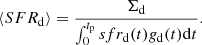
The top panel of Fig. 3 shows the vertical and radial thin-disk density profiles predicted for 0.25-Gyr age bins. The vertical profiles are calculated for the solar radius. The radial profiles correspond to the midplane densities.
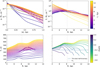 |
Fig. 3. Radial and vertical structure of the thin disk according to the JJ model realisation TM1 (Sect. 3.1). Top: vertical and radial density profiles of the thin-disk mono-age sub-populations. The vertical density profiles correspond to the solar radius. Bottom: radial variation in scale heights of the thin-disk mono-age and mono-abundance sub-populations. |
The vertical density profiles for ages ≳4 Gyr demonstrate a monotonous decline with z. Though the youngest age bins are characterised by a more complex vertical density fall-off, we can identify several regimes with the different slopes. This behaviour is a direct consequence of the model input. In TM1, the mono-age sub-population fractions associated with the extra SFR peaks are more dynamically heated than their remaining parts following AVR (see the bottom panel of Fig. 2). Thus, the youngest age bins consist of several kinematically different sub-components, and the final shape of the vertical profile depends on these sub-components’ fractions and W-velocity dispersions. We observed this multi-slope shape of the vertical density profile for the local A-type star sample selected from the Gaia DR2 (Paper IV).
As to the radial profiles, we see that though the overall thin-disk surface density law is assumed to be exponential (Eq. (12) and Fig. 1), the profiles of individual age bins can significantly deviate from this shape. The oldest thin-disk populations have quasi-exponential radial profiles, though two-slope exponential law can provide a more accurate fit in this case. Starting from ∼8–9 Gyr, profiles have a peak at the radius, which shifts to the outer disk as the age decreases. This reflects the lack of young populations in the inner disk due to the chosen SFR: young thin-disk stars formed mostly at large radii. The density profiles of the youngest populations have additional overdensities located around the extra SFR peaks’ mean radii Rp.
This result is in a good agreement with the observed radial surface density trends in the MW disk. Bovy et al. (2016) and Mackereth et al. (2017) used APOGEE data to study the radial disk structure in terms of mono-age and mono-abundance populations. They find that the radial surface density profiles of both mono-age and mono-abundance low-α populations (which correspond to the chemically defined thin disk) are at best described by a broken exponential law. High-α populations representing the thick disk show no significant change of the slope over the studied distance range of 3–15 kpc. Similar radial structure follows from the JJ-model predictions (see the upper-right panel of Fig. 1, which shows radial surface density profiles of the mono-age thin-disk sub-populations). As to the thick disk in the JJ model, its mono-age and mono-abundance sub-populations are all single exponential profiles with a slope of the overall thick-disk radial profile shown in Fig. 1. Amôres et al. (2017) used BGM in combination with the 2MASS data to study the disk properties such as warp, flare, and populations’ scale lengths. They find that the thin-disk scale length is age dependent, with the youngest populations characterised by the largest scale lengths. The JJ model also recreates this trend which naturally follows from the inside-out disk growth scenario implied by the shape of our adopted SFR (Fig. 2). The same negative correlation of scale length with age and double-slope radial profiles of the thin-disk mono-age sub-populations are predicted by hydrodynamic simulations of the MW-like galaxies in Minchev et al. (2015).
3.2.2. Scale heights
The lower panel of Fig. 3 displays the radial change of the thin-disk scale heights calculated for different age and metallicity bins.
One of the interesting results of our modelling is that the mono-age populations flare even though the overall thickness of the thin disk is the same at all radii (dashed blue line in the lower-left panel of Fig. 3). The same effect of mono-age sub-populations flaring when the overall disk thickness is approximately constant is reproduced in Minchev et al. (2015). The effect is generated by an interplay of two factors: (1) the inner disk is on average more dynamically heated than the outer disk, and (2) the relative fraction of old-to-young stars decreases with increasing radius. Similarly, Mackereth et al. (2017) find flaring for essentially all mono-age sub-populations of the low-α APOGEE stars. As follows from Fig. 3, for the youngest and oldest age bins in the range of 4–14 kpc scale heights change from approximately 80 pc to 180 pc and from 440 pc to 700 pc, respectively. Thus, flaring scale lengths predicted by this model lay in the range of ∼12.5–17 kpc. However, Mackereth et al. (2017) report a trend for the flaring with age that is the oppositive of that given by the JJ model: according to the APOGEE data, the youngest populations flare the most. Mackereth et al. (2017) suggest that at the early stage of the disk formation flaring could be suppressed by the active accretion. This topic may be deeper investigated in our future works. Another feature is the presence of a peak in the scale-height profiles of the young populations due to the contribution of kinematically hot SFR peaks’ sub-populations. Also, we see an opposite ‘response’ in the scale heights of older ages around 9 kpc: here scale heights grow slower than we would expect from the trends up to this radius. We can attribute this behaviour to the SFR re-normalisation. As explained in Sect. 2.3.3, we re-normalise the total thin-disk SFR to the same Σd after adding extra peaks. In the case of TM1 we have two extra peaks at young ages, that is, we increase the contribution of the young sub-populations by decreasing contributions of all other ages. And though these young sub-populations are partly more heated than prescribed by AVR, the modified age balance may in some age bins result in a more plane-concentrated matter distribution than we could expect without extra SFR peaks.
As mono-age populations are not easily observable, it is useful to convert them to mono-abundance populations using the AMR function (Sect. 4.2.4). At the lower right panel of Fig. 3 we show the radial variation of the thin-disk scale heights calculated in 10 metallicity bins on the interval from −0.7 to 0.3 dex with a 0.1-dex bin width. We see that the scale-height radial profiles of the metal-poor populations closely follow the corresponding profiles of the oldest age bins. In other words, mono-abundance thin-disk populations can be also considered as mono-age when the metallicity is low. To the same conclusion arrived Minchev et al. (2017) who investigated the relationship between mono-age and mono-abundance sub-populations using the chemodynamical model of the MW-like galaxy with inside-out disk growth. As the metallicity increases, mono-abundance populations begin to include more ages, and the corresponding age distributions depend on radius. For metallicities > − 0.2 dex, profiles do not span over the whole range of galactocentric distances, but end at some radius, and this stop point moves to the inner disk as the metallicity increases. This happens because a given metallicity ceases to be present starting from some radius, according to our simple chemical evolution model. Due to the multi-age composition of most of the mono-abundance populations, the flaring trend is observed only for most metal-poor bins, while for other mono-abundance sub-populations it is suppressed. Also, in Minchev et al. (2017) the authors find that flaring is not prominent in most of the metallicity bins because of their negative radial age gradient. On the other side, radial surface density profiles of APOGEE mono-abundance sub-populations show flaring in almost all metallicity bins (Bovy et al. 2016; Mackereth et al. 2017). This can be viewed as a lack of flaring in the overall thin-disk profile, which can be easily included into the model. Also, this can point to the lack of some fundamental physical process, such as radial migration, that would relocate some fraction of stars from the inner to the outer disk and thus lead to an extra flaring.
As to the thick disk, our non-flaring disk is consistent with the observed nearly constant thickness of the high-α APOGEE mono-abundance sub-populations (Bovy et al. 2016; Mackereth et al. 2017), properties of the thick disk constrained with the SDSS data in the BGM framework (Robin et al. 2014), and the thick disk simulated in Minchev et al. (2015).
3.2.3. Vertical kinematics
Following a routine described in Sect. 2.9, we converted the modelled densities into SA using PARSEC isochrones. Then we created several mock samples of the well-defined observable populations, such as A, F, and RC stars and G and K dwarfs. All of them, except RC stars, were selected by simple cuts applied to the effective temperature and surface gravity (in the case of dwarfs). Our RC modelling routine is described in Sect. 4.2.2.
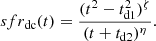
Figure 4 shows W-velocity distribution functions of these five mock thin-disk samples calculated for the solar radius for |z|< 2 kpc. As expected, A- and F-star samples consisting exclusively or predominantly from the young populations, have f(|W|) with a prominent core. The main sequence (MS) stars, G and K dwarfs, have velocity distributions with a much more significant contribution of the dynamically heated stars. Interestingly, the RC sample consisting of a mixture of different ages with a significant fraction of young populations, has f(|W|) essentially indistinguishable from the one of the MS samples (also see Figs. 8 and 10 in Paper IV). For the current model realisation, this can be understood as follows: though the RC sample contains more young stars than G and K dwarfs, young populations of the SFR peaks also partly contribute to the tail of the velocity distribution, such that the resulting RC and G- and K-dwarf f(|W|) are very similar. Figure 4 is also representative for other modelled radii.
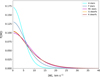 |
Fig. 4. Normalised W-velocity distribution functions of the different mock populations at the solar radius. |
4. AMR from APOGEE RC stars
In this section, we take the first step towards calibration of the generalised JJ model across the disk. We use the developed machinery to constrain the AMR function with the APOGEE data covering distances 4 kpc < R < 14 kpc. Motivated by the obtained results, we then develop a new analytic representation of the thin-disk AMR.
4.1. Sample selection
To constrain the AMR across a wide range of galactocentric distances, we use the latest data release, DR16, of the APOGEE RC catalogue (Bovy et al. 2014; Ahumada et al. 2020). The APOGEE RC catalogue comprises a kinematically unbiased sample of 39 675 bright stars spanning over a large fraction of the Galactic disk. As the luminosity of RC stars depends very little on their chemical composition and age, they can play the role of standard candles. Thus, for the RC stars, it is possible to obtain robust photometric distances – distance uncertainties of the APOGEE RC stars are reported to be less than ∼5% (Bovy et al. 2014). Using heliocentric distances provided in the RC catalogue, we calculated Galactic cylindrical coordinates R and z (the adopted position of the Sun (R⊙, z⊙) is the same as in Table 2).
It is well known that when projected onto [α/Fe]-[Fe/H] chemical abundance plane, the MW disk stars form two distinct sequences, which are associated with the thin- and thick-disk populations. We used a simple criterion to separate low- and high-α sequences, similar to the one adopted in Paper IV12 (Fig. 5, top panel):
![Mathematical equation: $$ \begin{aligned} [\alpha /\mathrm{Fe}] = {\left\{ \begin{array}{ll} \ 0.04,&\mathrm{[Fe/H]} > 0.1 \\ \ -0.14 \, \mathrm{[Fe/H]} + 0.05,&-0.6 < \mathrm{[Fe/H]} < 0.1 \\ \ 0.14,&\mathrm{[Fe/H]} < -0.6. \end{array}\right.} \end{aligned} $$](/articles/aa/full_html/2022/10/aa43780-22/aa43780-22-eq25.gif) (19)
(19)
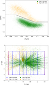 |
Fig. 5. Selection of the APOGEE RC samples. Top: low-α (green) and high-α (orange) RC sequences. The separation border corresponding to Eq. (19) is shown with dashed black line. Bottom: selected low-α and high-α RC populations in the R-z plane. Dashed lines mark the adopted limits for the galactocentric distance and height. The radial binning of the low-α population corresponds to run0 (see text). The adopted position of the Sun is marked with a yellow dot. |
To eliminate halo stars, we applied a cut [Fe/H] > −1. From the remaining subsample, we took stars with |z| < 2 kpc, both for the high- and low-α population. Finally, we defined the radial range of the samples. Here we keep in mind that the high-α population is known to be chemically homogeneous, while the low-α MD systematically change with galactocentric distance. Therefore, in case of high-α sample, we selected stars with galactocentric distances 4 kpc < R < 14 kpc and did not apply radial binning (red dashed box at the lower panel of Fig. 5). For the low-α stars, we used a grid of 1-kpc bins centred at 4.5, 5.5, …, 13.5 kpc (blue dashed lines). We later refer to this grid as run0. In order to eliminate an impact of binning on the reconstructed AMR, we used four additional grids for the low-α sample (Sect. 4.2): three grids shifted with respect to the initial one by +0.25, +0.5, and +0.75 kpc (run1, run2, and run3, respectively) and a finer grid with 0.5-kpc bins centred at 4.25, 4.75, …, 13.75 kpc (run4). Also, we found that bins of these grids that partially lay at R > 14 kpc and contain fewer than ∼300 stars cannot provide enough data to set a robust constraint on the thin-disk AMR parameters. For this reason, we excluded such bins from our analysis.
In the selected samples, 95% of stars have a signal-to-noise ratio (S/N)≳50, so we did not apply any quality cuts. Our final RC samples contain 4444 (high-α) and 32 917 stars (low-α, run0).
It is also worthwhile to address the problem of extinction, which is known to be very significant in the Galactic plane at the large distances reached by our sample. As explained in Majewski et al. (2011), the APOGEE photometry is corrected for extinction with the help of the Rayleigh-Jeans colour excess (RJCE) method. The RJCE technique is based on sampling the spectral energy distribution (SED) in the Rayleigh-Jeans regime where the shape of stellar SED is essentially independent of its spectral type. Thus, extinction for each star can be robustly estimated by measuring the colour excess from its photometry in near- and mid-infrared bands. As the RC distances are based on the APOGEE photometry corrected for extinction, they are not biased. As reported in Bovy et al. (2014), uncertainties in extinction determination make only a minor contribution to the total error budget of the RC distances. The stellar parameters that were used to select the RC stars from the full APOGEE catalogue, such as metallicity, logg, Teff, were derived with the APOGEE Stellar Parameter and Chemical Abundances Pipeline (ASPCAP). The effect of reddening is suppressed in ASPCAP by working with the observed and template spectra that are continuum-normalised (García Pérez et al. 2016). Taking all this into account, we can conclude that no special measures need to be taken in our analysis to account for the extinction, and we can compare the APOGEE RC sample to our mock RC population simulated with the stellar parameters and distances not affected by extinction.
4.2. AMR reconstruction
Our approach for the AMR reconstruction is based on a direct comparison of the observed MDs to the modelled age distributions of some population and was explained in detail in Paper IV. Here we summarise its main steps as applied to this study.
First, we calculated the observed cumulative metallicity distribution functions (CMDFs) of the low- and high-α stars using the selected RC data samples. In the case of the low-α population, CMDF was obtained separately in the different radial bins.
Then assuming AMR for the thick disk (same at all radii) and for the thin disk (radially dependent) and working in the framework of the generalised JJ model, we derived the total vertical gravitational potential and the vertical density profile of the RC population at each radius. The density profile was then used to calculate the cumulative age distribution functions (CADFs) of the thin- and thick-disk RC stars within the selected R-z limits.
At the next step we compared the observed CMDFs to the predicted CADFs: we put in correspondence stellar metallicities and ages, and thus, arrived at the updated AMR of the thin- and thick-disk (radially dependent and the same for all R, respectively). To achieve self-consistency, we iterated over the last two steps until the obtained thin- and thick-disk AMR converged to a constant shape (∼3–5 iterations).
After that we fit the obtained thin- and thick-disk AMR with analytic functions. In the case of the thin disk, we investigated the radial trends of the AMR best-fit parameters and also fit them with simple laws. As a result, we obtained a ‘generalised’ thin-disk AMR fit, which is well-consistent with the originally reconstructed ‘raw’ AMR.
Finally, we performed a consistency test: calculated the thin- and thick-disk MDs of the RC stars using the updated AMR and compared these predictions to the data.
Each of these steps is described in more detail in the successive subsections.
4.2.1. Cumulative metallicity distributions
The CMDFs of the selected low- and high-α APOGEE RC stars are shown in Fig. 6. There are three distinct regimes that can be identified for all CMDFs: a rapid non-linear increase at low metallicities, linear part, and a non-linear deceleration in growth at high metallicities. Following Paper IV, we make a simplifying assumption: at each radius, chemical enrichment process was monotonous in time (i.e. the AMR of interest is a monotonously growing function of Galactic time). This implies that low- and high-metallicity tails of CMDFs correspond to old and young populations, respectively. Then the non-linear growth of a CMDF at low metallicities reflects a quick chemical enrichment at the beginning of the MW disk evolution when the SF processes, and therefore the enrichment of ISM with metals, were most intense. The non-linear shape of CMDF at the high-metallicity end is, however, puzzling in this framework, as we do not expect a significant increase in the ISM chemical enrichment rate at the present day and do not have observational data that imply that. So, in order to obtain the AMR that does not show any special behaviour at the present day, we represented the upper part of each CMDF as a convolution of the linear trend (monotonous chemical enrichment) with a Gaussian kernel (error model). The analytic form of such a convolution was given in Paper IV (Eq. (17)), and for the sake of completeness of narration, we show it here:
![Mathematical equation: $$ \begin{aligned}&C(\mathrm{[Fe/H]} ) = \frac{1}{2}\left[A\,\mathrm{Erf} \left(\frac{A}{B}\right) - \left(A - 1\right)\mathrm{Erf} \left(\frac{A-1}{B}\right) + 1 \right] \nonumber \\&\qquad \qquad \qquad + \frac{B}{2\sqrt{\pi }}\left[\exp {\left(-\frac{A^2}{B^2}\right)} - \exp {\left(-\frac{(A-1)^2}{B^2}\right)} \right]\!, \\&\mathrm{where} \quad A = k \cdot \mathrm{[Fe/H]} + b, \quad B = \sqrt{2} k \sigma _{\mathrm{[Fe/H]} }. \nonumber \end{aligned} $$](/articles/aa/full_html/2022/10/aa43780-22/aa43780-22-eq26.gif) (20)
(20)
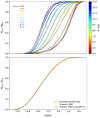 |
Fig. 6. CMDFs of the APOGEE RC samples. Top: low-α CMDFs calculated in the different radial bins (run0 grid). Dotted coloured curves are CMDFs with extrapolated linear parts. Dashed black curves are C([Fe/H]), convolutions of the ‘deconvolved’ CMDFs with the Gaussian kernel (Eq. (20)). The kernel dispersions σ[Fe/H] are shown on the plot with the same colour coding. Bottom: same as the top panel, but for the high-α stars and no radial binning. |
Parameters k and b are slope and intercept of the linear part of CMDF, and σ[Fe/H] is a dispersion of the Gaussian kernel.
For each CMDF, we selected the linear part and obtained parameters k and b (0.4 < Ncum/Ntot < 0.8 for the low-α stars with bin centres at R < 7 kpc and 0.3 < Ncum/Ntot < 0.7 at all other radii and for the high-α population). Then, with k and b known, we fit the upper parts of CMDFs with Eq. (20) and thus determined σ[Fe/H] – dispersion required to reproduce the high-metallicity CMDF tail with the Gaussian error model. The corresponding values of σ[Fe/H] for the different R bins of the low-α population are displayed at the upper panel of Fig. 6. Later we used these values to model the high-metallicity MD parts. The ‘deconvolved’ upper parts of CMDFs are shown with dotted lines in Fig. 6.
The error model can represent different aspects (or be a result of their interplay): (1) systematic errors at the metal-rich end or (2) the presence of the real stars that have migrated to a given volume from the inner radii and therefore have an imprint of the different environment and probably do not belong to the youngest population. Which of these interpretations is correct, and to which extent, we do not investigate within our approach.
4.2.2. RC star modelling
TM0 framework. For the AMR reconstruction, we used a simpler version of the test realisation of the generalised JJ model presented in Sect. 3.1. The most uncertain ingredient of TM1 is the extra SFR peaks at R ≠ R⊙. In order not to propagate this uncertainty to our results and also following Paper IV, we omitted the additional SFR peaks for the RC sample modelling. To initialise AMR at the second step of the AMR reconstruction scheme, we used the thin- and thick-disk AMR from Paper IV calibrated against the local APOGEE RC sample (Eqs. (21) and (22)). The thin-disk AMR was extended to other radii by assuming power-law radial variations of its four parameters. The power indices were chosen such that the radially dependent AMR predicted quicker and more intense chemical enrichment in the inner disk: k[Fe/H]d0 = −0.025, k[Fe/H]dp = −0.0875, krd = 0.005, kq = −0.03.
RC mock sample. To select the RC stars in TM0, we used the following criteria for the effective temperature, surface gravity, and luminosity: 4250 K < Teff< 5250 K, logg< 2.75, 1.65 < log(L/L⊙)< 1.85. These cuts determine a sample of RC contaminated by red giant branch (RGB) stars. To remove RGB stars, Bovy et al. (2014) use an additional sloping cut in logg, a linear function of the effective temperature and metallicity: logg < f(Teff, [Fe/H]). As we have already found in Paper IV (Eqs. (18)–(20)), the exact values of this cut’s slope and intercept depend on the stellar evolution library, and also on the population’s MD (i.e., on the assumed AMR). When visualised in (logg, logTeff, logL)-space, the pre-selected sample forms a fork-like structure, with the two hands being RC and RGB sequences. The f(Teff, [Fe/H]) criterion defines a plane that separates one sequence from another. In order to avoid the need to manually adapt the f(Teff, [Fe/H]) criterion each time we change the model parameters or isochrones, we introduced a numerical routine to separate the RC and RGB stars (included into the jjmodel code). After applying our routine to the pre-selected sample, we got a clean RC population. At the subsequent steps, we modified the vertical spatial densities of this complete sample to account for the geometry of the observational data (Sect. 4.2.3) and then used these vertical density profiles for the AMR reconstruction (Sect. 4.2.4).
4.2.3. Cumulative age distributions
To perform realistic modelling of some stellar population, it is important to properly take into account possible selection effects, so we address this question before modelling RC CADFs.
The R-z plot of our APOGEE samples in Fig. 5 (bottom) shows that the selected RC stars are distributed in space very unevenly. Indeed, the APOGEE survey does not provide a full sky coverage but targets a set of ‘grid’ and ‘non-grid’ pointings, whose selection is motivated by location of objects of special interest and goals of the different scientific projects, as well as some technical limitations (Zasowski et al. 2013, 2017). To observe spectra, fibre-plugged plates are used, such that each fibre corresponds to a certain area in the sky. As a result, space coverage of the APOGEE consists of so-called pencil beams probing the MW stellar populations within the selected directions (Wilson et al. 2019).
We can formulate this spatial selection in the following way: at each radius, the observed vertical number density law deviates from the real one, and the residual reflects the sample geometry (assuming that there are no other losses). In the JJ model, on the contrary, we by default work with complete populations whose vertical number density declines smoothly with z. So we need to understand whether the spatial irregularity of the APOGEE RC sample is relevant for the calculation of CADFs, and in which form it can be taken into account.
The thick disk is known to be a well-mixed population – quite homogeneous in age, chemical composition, and kinematics (Lee et al. 2011; Haywood et al. 2013; Hayden et al. 2015, 2020). Within the JJ-model framework, it is represented with a single isothermal population at each R. This implies that the predicted thick-disk age and MDs are the same at all heights at a given radius. Thus, even if the predicted thick-disk vertical number density law (complete sample) does not exactly follow the observed vertical distribution (‘pencil beams’), this cannot introduce any bias to the modelled age distribution, and therefore, no correction for the sample geometry is needed.
In the case of the thin disk, the situation is different. As we represent the thin disk with multiple isothermal populations, its kinematic, chemical, and age properties significantly change with z at a fixed R. Therefore, to model the realistic age distributions of the thin-disk APOGEE RC sample, it is important to properly account for the sample’s spatial geometry.
To do so, we use the following approach. At each radius, we calculated Ndata(|z|), a distribution of the observed thin-disk RC stars over |z| up to 2 kpc with a step of 50 pc. In the model, we do not model the real star counts, but predict the vertical number density of RC stars according to Eq. (18),  . To be able to compare modelled and observed quantities, we normalised both vertical laws to their midplane values. As
  , we arrived at the comparable quantities. The observed and predicted normalised vertical profiles are shown at the top panel of Fig. 7. We calculated the ratio:
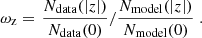 (21)
(21)
 |
Fig. 7. Spatial selection function of the thin-disk RC sample. Top: observed (green histogram) and predicted (blue curves) number density laws of a complete sample in R bins. Modelled profiles with the disk warp taken into account are shown in dashed blue. Both observed and modelled density laws are normalised to the midplane densities. Bottom: z weights calculated as a ratio of the observed to modelled profiles. The grey line marks ωz = 1, the case of a complete sample. |
At each |z|, quantity ωz shows by how much the observed vertical distribution of stars deviates from the vertical density law of a complete population. Assuming that TM0 predictions are entirely correct, this deviation reflects the observed sample’s incompleteness and geometry. Thus, we can use ωz to modify the modelled RC age distributions to mimic the geometry and incompleteness of the APOGEE RC sample.
For the reasons explained below in Sect. 4.2.4, we find it useful to test an impact of the warp on our modelling. We adopted a simple linear warp model from Chen et al. (2019). The normalised vertical number density laws and the relative weights ωz corresponding to TM0 with and without the warp are shown in Fig. 7. The mock RC CADFs calculated with TM0 without the warp and weights ωz taken into account are shown in Fig. 8. The displayed CADFs correspond to the 5th iteration (consistent with the reconstructed AMR in Sect. 4.2.4).
 |
Fig. 8. Normalised CADFs of the thick-disk (black curve) and thin-disk (colour-coded) RC sample. The thin-disk radial grid corresponds to run0. |
4.2.4. AMR fitting process
In Paper I–Paper IV, we used a logarithmic function to describe a monotonous increase of the thin-disk sub-populations’ metallicity with time, and in Paper IV we proposed a tanh-law for the AMR of the thick disk. In this study, we find that the shape of the thin-disk AMR is very different at the different R, ranging from a function with a steep increase at small t in the inner disk to a quasi-linear law in the outer disk (Fig. 9). Though our old log-law is well-suited for reproducing the local thin-disk AMR, it is unable to describe such a family of curves. Therefore, for the radially dependent AMR of the thin disk, we introduce a new seven-parameter tanh-function, which can be viewed as a more complex form of the thick-disk tanh-law. As before, the metallicity as a function of time for both thin and thick disk is expressed in the following form:
![Mathematical equation: $$ \begin{aligned} \mathrm{[Fe/H]} (t) = \mathrm{[Fe/H]} _0 + (\mathrm{[Fe/H]} _\mathrm{p} - \mathrm{[Fe/H]} _0) \cdot f(t), \end{aligned} $$](/articles/aa/full_html/2022/10/aa43780-22/aa43780-22-eq30.gif) (22)
(22)
 |
Fig. 9. Reconstructed AMR of the thin and thick disk (solid coloured and black lines, respectively) and their best fits (dashed lines; Eqs. (22)–(24), parameters from Table 3). |
where functions f(t) for the thin and thick disk are given by Eqs. (23) and (24)13, respectively:
 (23)
(23)
 (24)
(24)
Figure 9 shows the thin- and thick-disk AMR (solid curves), which we reconstructed following the procedure described in the previous sections. We note that AMR not only of the thick disk, whose SF ceased in the model ∼9 Gyr ago, but also of the thin disk does not extend to the present day. In the case of the thin disk, this reflects the age span of the modelled RC sample: depending on the radius, the last ∼0.5–5 Gyr of the thin-disk evolution are not represented by our sample (see age distributions in Fig. 8). We recovered the missing ages by fitting the reconstructed raw AMR and extrapolating these fits to the present day.
Fitting the thick-disk AMR with Eqs. (22) and (24) is straightforward. The obtained parameters are listed in Table 3, and the fitted AMR is shown in Fig. 9.
The analytic thin-disk AMR has to be a function of time t and galactocentric distance R. The presented thin-disk AMR equation, Eqs. (22) and (23), is a function of time only, as it describes the AMR shape at some fixed R. To add dependence on the distance, we assumed its parameters to be simple functions of R. Our tests showed that if all thin-disk AMR parameters are fitted simultaneously, then the corresponding generalised analytic AMR significantly deviates from the raw AMR, which we reconstructed based on the APOGEE data. To find the generalised AMR that is well-consistent with the raw reconstructed AMR, we fit parameters step by step in the following way.
Firstly, we fit the raw thin-disk AMR in each radial bin with Eqs. (22) and (23).
After that, we adopted analytic radial profiles for the obtained best-fit initial and present-day metallicity, [Fe/H]0 and [Fe/H]p. As one can see from [Fe/H]0 panel at Fig. 10, there is no clear radial trend and a large scatter. In order not to over-interpret the obtained results, we adopted a constant value for this parameter for all radii. [Fe/H]p manifests, on the contrary, a clear negative gradient on almost the whole interval of the examined galactocentric distances. In the inner disk, at R ≲ 6 kpc, the present-day thin-disk metallicity remains approximately constant. This change of [Fe/H]p slope can be related to the real physical processes, in particular, to the impact of bulge. Therefore, we modelled [Fe/H]p with a broken law, which is a constant at R < Rbr1 with Rbr1 = 6 kpc and linearly declines with radius at larger R. Then, treating [Fe/H]0 and [Fe/H]p as known, we again fit the raw AMR and updated the optimal values of the remaining five parameters (r1, r2, αω, t01, t02).
 |
Fig. 10. Best-fit parameters of the thin-disk AMR. Different colours and symbols correspond to the five radial grids (run0–run4). Vertical grey lines mark the break-point positions. Blue lines are the overall fits of the radial trends. |
During the fitting at the previous step, we searched for the best values of power indices r1 and r2 in the narrow non-overlapping intervals centred at 0.5 and 1.5, such that tanh-terms in Eqs. (22) and (23) dominate at different ages. We find that without deteriorating the fit quality, we can adopt for all radii r1 = 0.5 and r2 = 1.5. At this stage, we re-fit the AMR to update parameters (t01, t02, αω).
Next, we fit parameter αω with a linear profile and updated the remaining (t01, t02).
Finally, we adopted fits for parameters t01 and t02. Two bottom panels at Fig. 10 show their best-fit values at different R. It is clear that both of these parameters change with radius non-monotonously. At the same time, the value of metallicity predicted according to Eqs. (22) and (23) is very sensitive to t01 and t02. As a result, it is not possible to fit the obtained data points with a constant or linear trend as we did with [Fe/H]0 and αω and obtain a good fit of the raw AMR. For this reason, for both t01 and t02 we used three-slope broken linear laws.
Figure 10 shows the best values of five parameters of the thin-disk AMR, which we obtained using such a step-by-step fitting routine. We repeated this fitting procedure for our five R grids. Using different binning results in a scatter in the parameters’ radial trends, but overall the data points of all runs are well consistent with one another; therefore the generalised AMR that we defined based on these profiles is not biased by the choice of bin edges.
There is a distinct change of slope in both t01 and t02 trends around ∼10 kpc. In order to check whether this feature partially or fully originates from the absence of the warp in our model, we tested TM0 with the warp. It is already clear from Fig. 7 that the impact of warp starts to be noticeable only at R ≈ 13 kpc and is very small. The best-fit values corresponding to the AMR reconstruction with TM0 with the warp are essentially indistinguishable from the values obtained for the runs without the warp at Fig. 10. This essentially does not change if we use the model with the more pronounced warp from Poggio et al. (2020). From this we can at least conclude that the non-monotonous behaviour of t01 and t02 radial profiles in the outer disk is not related to the lack of warp in our model.
As a wrap-over, we applied the step-by-step fitting to the parameter values of run0–run4 collectively and obtained the final radial profiles of the AMR parameters (green lines on Fig. 10). At this stage, we also optimised the break-point positions for t01 and t02 by minimising a mean relative deviation between the real and fitted best parameter values:
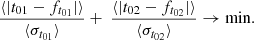
Here ft0i are the analytic profiles with some assumed break-point positions, σt0i is the dispersion. The calculation was performed in the R grid with bin centres at 4.5, 5.5, …, 14.5 kpc. We find that the optimal position of the second break is 9.75 kpc for both parameters, while the first break lies at 7.5 kpc and 6.25 kpc for t01 and t02, respectively. The break point at 6.25 kpc is very close to Rbr1 = 6 kpc, which we adopted for [Fe/H]p, as this parameter is strongly correlated with t02 (both affect the AMR shape at young ages). In order not to further complexify our analytic representation of the thin-disk AMR, we set the first break of t02 profile also to 6.0 kpc.
The obtained fits for the AMR parameters are listed in Table 3. The resulting generalised thin-disk AMR is plotted in Fig. 9 with dashed coloured curves. We see that the final AMR fit has a very good consistency with the raw reconstructed AMR.
4.2.5. Consistency test
To demonstrate the consistency between the APOGEE data and the JJ model after the AMR calibration, we predicted the RC MDs using the derived AMR and compared them to the observed metallicities. The MD modelling was performed in the full consistency with the approach used to reconstruct the AMR function. For the thick disk, MD was predicted for the mock RC population within the range of 4–14 kpc and at |z|< 2 kpc in the TM0 framework. For the thin disk, MDs were calculated separately in each radial bin, and the vertical densities of the modelled RC populations were weighted with ωz. We also added an error model as a post-processing step: each MD was converted into cumulative form, convolved with a Gaussian kernel of σ[Fe/H] as derived from the data (Fig. 6), and then transformed back to non-cumulative distribution. The resulting thin- and thick-disk MDs are shown in Figs. 11 and 12. Two types of step histograms correspond to TM0 predictions with the raw and generalised analytic AMR.
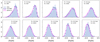 |
Fig. 11. Normalised observed and predicted MDs of the thin-disk RC sample calculated for the different radial bins. Dark blue and magenta step histograms are the JJ-model predictions that correspond to the raw reconstructed AMR and the generalised analytic AMR calculated according to Eqs. (22) and (23) with the best-fit parameters from Table 3. |
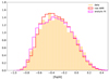 |
Fig. 12. Same as in Fig. 11, but for the thick disk. Both observed and predicted MDs correspond to the range of galactocentric distances 4–14 kpc. |
We see that the model and data are well consistent in terms of the overall shapes and peak positions of the distributions. The maximum shift that we report between the modelled and observed MD is only ∼0.05 dex.
5. Discussion
The goal of the JJ model is to provide a flexible modelling tool for the main body of the MW disk in terms of stellar populations and their properties. We model the axisymmetric disk in dynamical equilibrium. In order to allow the investigation of the Galaxy evolution over the full age range, we represent the stellar content of the disk by sequences of stellar sub-populations with a high time resolution of 25 Myr. This ansatz is complementary to the BGM model, which tries to incorporate all MW features including the bar, spiral structure, and the warp at the cost of a restricted time resolution. The input JJ-model functions SFR, AVR, and AMR are relatively simple functions of galactocentric distance and time (i.e. age). The IMF is assumed to be universal, but this could easily be made a function of metallicity in the framework of the JJ model (see Sect. 2.3.1).
5.1. Model properties and limitations
The JJ model provides predictions for the density distribution, vertical velocity distribution function, age distributions, and MD function for stellar subsamples (along the MS, RC stars, etc.). The parameters of the input functions are constrained by comparison of these predictions with corresponding observed samples. We did not use observed samples with individual age determinations, because they are still very restricted and may have significant biases. Therefore, direct age determinations can be used as independent tests of the model (or our model can be used as a tool for deriving age distributions of stellar populations). We only remark here that to perform a robust model-to-data comparison, the impact of dust must be taken into account: a three-dimensional extinction map can be used to redden our synthetic photometry to compare to the data (forward modelling, Sysoliatina et al. 2018), or the data can be preliminary de-reddened and then compared to the model (as in Paper IV). Also, the selection function of the sample needs to be thoroughly scrutinised to include the corresponding selection effects to the model.
Since the JJ model contains only axisymmetric populations in dynamical equilibrium, it can be used to characterise the properties of model-to-data deviations, such as the spiral arms and the warp. Also, due to the modular design of the code, simple spiral arm or warp models can be implemented. As an example, we tested the impact of the warp on the AMR derivation and found no significant differences (see Sect. 4.2.4).
The SFR, AVR, and AMR describe the present-day properties of stellar sub-populations at the current galactocentric distance. All three functions depend on each other for the derivation of the present-day distribution functions to be consistent with observations. Also the stellar birth places do not appear explicitly in our model. Only in the limiting case of negligible radial migration (blurring and churning), the time- and radially dependent SFR is the star formation history at radius R, the AVR represents the heating function, and the AMR corresponds to the metal enrichment law. In the case of a significant radial migration impact, these input functions can be viewed as the results of a convolution of the true SFR, AVR, and AMR with the radial migration model. In Paper IV, we addressed this topic when discussing physical meaning of the reconstructed local SFR of the thin disk. Assuming that the impact of migration is a function of time, we can formulate this the other way: specify a range of radii that are represented by a particular age interval of the SFR, AVR, or AMR.
Additionally, the JJ model can be combined with the Chempy code to derive the chemical enrichment history at each radius including the gas infall and abundances of other elements.
5.2. AMR and radial migration
Abundance distributions of different elements play a fundamental role in determining the evolution of galaxies. Here we used only the iron abundance and the α enhancement in a simple way to separate the thin and thick disk and derive the AMRs. Many other elements are available to test the local enrichment model without radial migration. If radial migration is relevant, then the interpretation of the AMR and the other input functions is more complex as we explained above. The unique AMR, which we derived, corresponds to the mean metallicity as a function of age, and the underlying real AMR is a two-dimensional distribution as derived in many publications based on individual stellar ages (e.g., Bergemann et al. 2014). Our findings for the AMR are in general comparable to the picture presented in Feuillet et al. (2019) where the disk AMR was reconstructed at different R and z based on the Gaia DR2 and APOGEE data. They also see a significant variation of the AMR across the disk with the outer disk being more metal-poor. Their spatial age distribution gives evidence for disk flaring, which we also reproduce in our model.
Local mixing (blurring) produced by the non-circularity of the orbits can be taken into account by replacing the current radius by the guiding radius of the orbit. For the population properties at a given current radius a distribution of guiding radii has to be derived. In a similar way, radial migration working over larger distances via resonances (churning) can be modelled by replacing the guiding radii by distributions of birth radii, which define the efficiency of the migration process. In both cases, the main challenge is to take into account the correlations between different quantities due to the radial gradients in ages, densities, and metallicities.
In order to explain the large spread of abundances in the [α/Fe]-[Fe/H] plane, local enrichment models can be combined with radial migration (Schönrich & Binney 2009; Kubryk et al. 2015; Hayden et al. 2015; Johnson et al. 2021). Minchev et al. (2018) used N-body simulation model for a MW-like galaxy extended by a local chemical enrichment model to derive the evolution and enrichment history of the stellar disk based on a simple radial migration model. Recently, Xiang & Rix (2022) investigated the early MW evolution based on the ages and abundances of about 250 000 subgiant stars. They find a well-mixed α-enhanced thick disk with a similar early formation and enrichment as used in our model, but with an even more extended formation history of 4 Gyr and a higher maximum metallicity. Our thin-disk model corresponds to their dominating low-α evolution sequence. For a more detailed comparison the spatial distribution as a function of galactocentric radii needs to be analysed.
6. Conclusions
We have presented a publicly available update of our semi-analytic MW disk model, which is based on an iterative solving of the Poisson equation and recovers a self-consistent potential-density pair independently at each radius14. We generalised the local JJ model previously calibrated against the Gaia DR2 sample (Paper IV) by introducing radial variation to such input functions as the thin-disk SFR, AVR, and AMR. Our test model, which implies inside-out disk growth, is able to mimic known trends in the MW disk structure, such as broken exponential radial profiles and flaring of the mono-age sub-populations.
As a first step towards the global calibration of the JJ model, we reconstructed the AMR using the extended APOGEE RC sample. We find that the shape of the thin-disk AMR changes a lot within the considered range of galactocentric distances, 4–14 kpc, so we introduced a new analytic function that can reproduce this variation, a seven-parameter double-tanh law.
Applicable to a large volume, 4 kpc ≲R≲ 14 kpc and |z|≲2 kpc, the model can test different SFR shapes, disk flaring, IMFs, and AMRs. The JJ model is characterised by a fine time resolution of 25 Myr which can also be combined with a fine spatial resolution within the allowed range of R and z. Thus, the JJ model complemented by the PARSEC, MIST, and BaSTI isochrones can be used for recovering disk evolution, creating MW mock catalogues, or revealing the spiral structure and any other density deviations from the smooth axisymmetric disk.
See Table 1 for the list of abbreviations.
Throughout this paper, subscripts ‘d’, ‘t’, ‘sh’, ‘dh’, ‘H2’, and ‘HI’ stand for the thin disk, thick disk, stellar halo, DM halo, molecular and atomic gas, respectively. To avoid confusion, we also apply the following index notation. Index i is reserved for the MW components; mono-age isothermal sub-populations of the MW components are associated with index j; index k corresponds to extra thin-disk SFR peaks (Sect. 2.3.3); finally, stellar assemblies (Sect. 2.9) are used with index l.
This equation in Paper IV contains a typo; parameters η and ζ should be interchanged
As in the previous papers of this series we only considered the local volume, all model parameters were by default local and no subscript was used to indicate that. Now we explicitly mark local parameters by ‘⊙’ sign to distinguish between the values in the solar neighbourhood and at other galactocentric distances.
In our previous work, we used an older release of the APOGEE RC catalogue, DR14, so the given coefficients of Eq. (19) do not exactly match the corresponding coefficients in Paper IV (Eq. (6)), this is related to the difference in DR14 and DR16 calibrations.
In Paper IV, we presented the thick-disk f(t) without the normalisation factor as t0 ≈ 1, and thus, tanh(tp/t0) → 1 and can be dropped. Here we show the normalisation for the sake of consistency with Eq. (23).
Github repository of the jjmodel code: https://github.com/askenja/jjmodel
Acknowledgments
This work was supported by the Deutsche Forschungsgemeinschaft (DFG, German Research Foundation) – Project-ID 138713538 – SFB 881 (‘The Milky Way System’, subproject A06). This research made use of Python packages SciPy (Virtanen et al. 2020) and NumPy (Van Der Walt et al. 2011), a Python library for publication quality graphics matplotlib (Hunter 2007), a community-developed core Python package for Astronomy Astropy (Astropy Collaboration 2013, 2018), a Python mini-package fast-histogram (https://github.com/astrofrog/fast-histogram), as well as an interactive graphical viewer and editor for tabular data TOPCAT (Taylor 2005). We also thank Akash Vani, Oleksiy Golubov, and our anonymous referee for their comments which helped to improve scientific quality and clarity of the paper.
References
- Abazajian, K. N., Adelman-McCarthy, J. K., Agüeros, M. A., et al. 2009, ApJS, 182, 543 [Google Scholar]
- Ahumada, R., Prieto, C. A., Almeida, A., et al. 2020, ApJS, 249, 3 [Google Scholar]
- Amôres, E. B., Robin, A. C., & Reylé, C. 2017, A&A, 602, A67 [NASA ADS] [CrossRef] [EDP Sciences] [Google Scholar]
- Astropy Collaboration (Robitaille, T. P., et al.) 2013, A&A, 558, A33 [NASA ADS] [CrossRef] [EDP Sciences] [Google Scholar]
- Astropy Collaboration (Price-Whelan, A. M., et al.) 2018, AJ, 156, 123 [Google Scholar]
- Bahcall, J. N. 1984, ApJ, 276, 156 [NASA ADS] [CrossRef] [Google Scholar]
- Banerjee, S., & Kroupa, P. 2012, A&A, 547, A23 [NASA ADS] [CrossRef] [EDP Sciences] [Google Scholar]
- Bartko, H., Martins, F., Trippe, S., et al. 2010, ApJ, 708, 834 [Google Scholar]
- Bastian, N., Covey, K. R., & Meyer, M. R. 2010, ARA&A, 48, 339 [NASA ADS] [CrossRef] [Google Scholar]
- Bennett, M., & Bovy, J. 2019, MNRAS, 482, 1417 [NASA ADS] [CrossRef] [Google Scholar]
- Bergemann, M., Ruchti, G. R., Serenelli, A., et al. 2014, A&A, 565, A89 [NASA ADS] [CrossRef] [EDP Sciences] [Google Scholar]
- Bienayme, O., Robin, A. C., & Creze, M. 1987, A&A, 180, 94 [NASA ADS] [Google Scholar]
- Bienaymé, O., Leca, J., & Robin, A. C. 2018, A&A, 620, A103 [NASA ADS] [CrossRef] [EDP Sciences] [Google Scholar]
- Binney, J., & Tremaine, S. 2008, Galactic Dynamics (Princeton Univ. Press) [Google Scholar]
- Bizyaev, D., & Mitronova, S. 2002, A&A, 389, 795 [NASA ADS] [CrossRef] [EDP Sciences] [Google Scholar]
- Bland-Hawthorn, J., & Gerhard, O. 2016, ARA&A, 54, 529 [NASA ADS] [CrossRef] [Google Scholar]
- Bovy, J., Nidever, D. L., Rix, H.-W., et al. 2014, ApJ, 790, 127 [CrossRef] [Google Scholar]
- Bovy, J., Rix, H.-W., Schlafly, E. F., et al. 2016, ApJ, 823, 30 [NASA ADS] [CrossRef] [Google Scholar]
- Bressan, A., Marigo, P., Girardi, L., et al. 2012, MNRAS, 427, 127 [NASA ADS] [CrossRef] [Google Scholar]
- Buder, S., Sharma, S., Kos, J., et al. 2021, VizieR Online Data Catalog: J/MNRAS/506/150 [Google Scholar]
- Chen, X., Wang, S., Deng, L., et al. 2019, Nat. Astron., 3, 320 [NASA ADS] [CrossRef] [Google Scholar]
- Choi, J., Dotter, A., Conroy, C., et al. 2016, ApJ, 823, 102 [Google Scholar]
- Czekaj, M. A., Robin, A. C., Figueras, F., Luri, X., & Haywood, M. 2014, A&A, 564, A102 [NASA ADS] [CrossRef] [EDP Sciences] [Google Scholar]
- Dal Tio, P., Mazzi, A., Girardi, L., et al. 2021, MNRAS, 506, 5681 [NASA ADS] [CrossRef] [Google Scholar]
- Dotter, A. 2016, ApJS, 222, 8 [Google Scholar]
- Eisenstein, D. J., Weinberg, D. H., Agol, E., et al. 2011, AJ, 142, 72 [Google Scholar]
- Feuillet, D. K., Frankel, N., Lind, K., et al. 2019, MNRAS, 489, 1742 [Google Scholar]
- Gaia Collaboration (Prusti, T., et al.) 2016, A&A, 595, A1 [NASA ADS] [CrossRef] [EDP Sciences] [Google Scholar]
- Gaia Collaboration (Brown, A. G. A., et al.) 2018, A&A, 616, A1 [NASA ADS] [CrossRef] [EDP Sciences] [Google Scholar]
- Gaia Collaboration (Brown, A. G. A., et al.) 2021, A&A, 649, A1 [NASA ADS] [CrossRef] [EDP Sciences] [Google Scholar]
- García Pérez, A. E., Allende Prieto, C., Holtzman, J. A., et al. 2016, AJ, 151, 144 [Google Scholar]
- Girardi, L. 2016, Astron. Nachr., 337, 871 [NASA ADS] [CrossRef] [Google Scholar]
- Girardi, L., Groenewegen, M. A. T., Hatziminaoglou, E., & da Costa, L. 2005, A&A, 436, 895 [NASA ADS] [CrossRef] [EDP Sciences] [Google Scholar]
- GRAVITY Collaboration (Abuter, R., et al.) 2019, A&A, 625, L10 [NASA ADS] [CrossRef] [EDP Sciences] [Google Scholar]
- Guszejnov, D., Hopkins, P. F., & Ma, X. 2017, MNRAS, 472, 2107 [NASA ADS] [CrossRef] [Google Scholar]
- Hallakoun, N., & Maoz, D. 2021, MNRAS, 507, 398 [NASA ADS] [CrossRef] [Google Scholar]
- Hayden, M. R., Bovy, J., Holtzman, J. A., et al. 2015, ApJ, 808, 132 [Google Scholar]
- Hayden, M. R., Bland-Hawthorn, J., Sharma, S., et al. 2020, MNRAS, 493, 2952 [Google Scholar]
- Haywood, M., Di Matteo, P., Lehnert, M. D., Katz, D., & Gómez, A. 2013, A&A, 560, A109 [NASA ADS] [CrossRef] [EDP Sciences] [Google Scholar]
- Hidalgo, S. L., Pietrinferni, A., Cassisi, S., et al. 2018, ApJ, 856, 125 [Google Scholar]
- Hunter, J. D. 2007, Comput. Sci. Eng., 9, 90 [NASA ADS] [CrossRef] [Google Scholar]
- Jahreiß, H., & Wielen, R. 1997, in ESA SP-402: HIPPARCOS ’97. Presentation of the Hipparcos and Tycho Catalogues and the First Astrophysical Results of the Hipparcos Space Astrometry Mission, eds. B. Battrick, M. A. C. Perryman, & P. L. Bernacca (Noordwijk: ESA), 675 [Google Scholar]
- Johnson, J. W., Weinberg, D. H., Vincenzo, F., et al. 2021, MNRAS, 508, 4484 [NASA ADS] [CrossRef] [Google Scholar]
- Just, A., & Jahreiß, H. 2010, MNRAS, 402, 461 [NASA ADS] [CrossRef] [Google Scholar]
- Just, A., Gao, S., & Vidrih, S. 2011, MNRAS, 411, 2586 [NASA ADS] [CrossRef] [Google Scholar]
- Kalari, V. M., Carraro, G., Evans, C. J., & Rubio, M. 2018, ApJ, 857, 132 [CrossRef] [Google Scholar]
- Kalberla, P. M. W., & Dedes, L. 2008, A&A, 487, 951 [NASA ADS] [CrossRef] [EDP Sciences] [Google Scholar]
- Kalberla, P. M. W., Kerp, J., Dedes, L., & Haud, U. 2014, ApJ, 794, 90 [NASA ADS] [CrossRef] [Google Scholar]
- Kramer, E. D., & Randall, L. 2016, ApJ, 829, 126 [NASA ADS] [CrossRef] [Google Scholar]
- Kroupa, P. 2020, in Star Clusters: From the Milky Way to the Early Universe, eds. A. Bragaglia, M. Davies, A. Sills, & E. Vesperini, 351, 117 [NASA ADS] [Google Scholar]
- Kubryk, M., Prantzos, N., & Athanassoula, E. 2015, A&A, 580, A126 [NASA ADS] [CrossRef] [EDP Sciences] [Google Scholar]
- Kunder, A., Kordopatis, G., Steinmetz, M., et al. 2017, AJ, 153, 75 [Google Scholar]
- Lee, Y. S., Beers, T. C., An, D., et al. 2011, ApJ, 738, 187 [NASA ADS] [CrossRef] [Google Scholar]
- Lindegren, L., Lammers, U., Bastian, U., et al. 2016, A&A, 595, A4 [NASA ADS] [CrossRef] [EDP Sciences] [Google Scholar]
- Mackereth, J. T., Bovy, J., Schiavon, R. P., et al. 2017, MNRAS, 471, 3057 [Google Scholar]
- Maíz Apellániz, J., & Weiler, M. 2018, A&A, 619, A180 [NASA ADS] [CrossRef] [EDP Sciences] [Google Scholar]
- Majewski, S. R., Zasowski, G., & Nidever, D. L. 2011, ApJ, 739, 25 [NASA ADS] [CrossRef] [Google Scholar]
- Majewski, S. R., Schiavon, R. P., Frinchaboy, P. M., et al. 2017, AJ, 154, 94 [NASA ADS] [CrossRef] [Google Scholar]
- Marigo, P., Girardi, L., Bressan, A., et al. 2017, ApJ, 835, 77 [Google Scholar]
- McKee, C. F., Parravano, A., & Hollenbach, D. J. 2015, ApJ, 814, 13 [NASA ADS] [CrossRef] [Google Scholar]
- Michalik, D., Lindegren, L., & Hobbs, D. 2015, A&A, 574, A115 [NASA ADS] [CrossRef] [EDP Sciences] [Google Scholar]
- Minchev, I., Martig, M., Streich, D., et al. 2015, ApJ, 804, L9 [NASA ADS] [CrossRef] [Google Scholar]
- Minchev, I., Steinmetz, M., Chiappini, C., et al. 2017, ApJ, 834, 27 [Google Scholar]
- Minchev, I., Anders, F., Recio-Blanco, A., et al. 2018, MNRAS, 481, 1645 [NASA ADS] [CrossRef] [Google Scholar]
- Mor, R., Robin, A. C., Figueras, F., Roca-Fàbrega, S., & Luri, X. 2019, A&A, 624, L1 [NASA ADS] [CrossRef] [EDP Sciences] [Google Scholar]
- Nakanishi, H., & Sofue, Y. 2016, PASJ, 68, 5 [NASA ADS] [CrossRef] [Google Scholar]
- Offner, S. S. R., Clark, P. C., Hennebelle, P., et al. 2014, in Protostars and Planets VI, eds. H. Beuther, R. S. Klessen, C. P. Dullemond,&T. Henning, 53 [Google Scholar]
- Paxton, B., Bildsten, L., Dotter, A., et al. 2011, ApJS, 192, 3 [Google Scholar]
- Paxton, B., Cantiello, M., Arras, P., et al. 2013, ApJS, 208, 4 [Google Scholar]
- Paxton, B., Marchant, P., Schwab, J., et al. 2015, ApJS, 220, 15 [Google Scholar]
- Pieres, A., Girardi, L., Balbinot, E., et al. 2020, MNRAS, 497, 1547 [NASA ADS] [CrossRef] [Google Scholar]
- Poggio, E., Drimmel, R., Andrae, R., et al. 2020, Nat. Astron., 4, 590 [NASA ADS] [CrossRef] [Google Scholar]
- Read, J. I. 2014, J. Phys. G Nucl. Phys., 41, 063101 [Google Scholar]
- Reid, M. J., & Brunthaler, A. 2005, in Future Directions in High Resolution Astronomy, eds. J. Romney, & M. Reid, ASP Conf. Ser., 340, 253 [Google Scholar]
- Riello, M., De Angeli, F., Evans, D. W., et al. 2021, A&A, 649, A3 [NASA ADS] [CrossRef] [EDP Sciences] [Google Scholar]
- Robin, A. C., Reylé, C., Derrière, S., & Picaud, S. 2003, A&A, 409, 523 [NASA ADS] [CrossRef] [EDP Sciences] [Google Scholar]
- Robin, A. C., Reylé, C., Fliri, J., et al. 2014, A&A, 569, A13 [CrossRef] [EDP Sciences] [Google Scholar]
- Robin, A. C., Reylé, C., Marshall, D. J., & Schultheis, M. 2012, Astrophys. Space Sci. Proc., 26, 171 [NASA ADS] [CrossRef] [Google Scholar]
- Robin, A. C., Bienaymé, O., Fernández-Trincado, J. G., & Reylé, C. 2017, A&A, 605, A1 [NASA ADS] [CrossRef] [EDP Sciences] [Google Scholar]
- Ruiz-Lara, T., Gallart, C., Bernard, E. J., & Cassisi, S. 2020, Nat. Astron., 4, 965 [NASA ADS] [CrossRef] [Google Scholar]
- Rybizki, J., & Just, A. 2015, MNRAS, 447, 3880 [NASA ADS] [CrossRef] [Google Scholar]
- Rybizki, J., Just, A., & Rix, H.-W. 2017, A&A, 605, A59 [NASA ADS] [CrossRef] [EDP Sciences] [Google Scholar]
- Sahlholdt, C. L., Feltzing, S., & Feuillet, D. K. 2022, MNRAS, 510, 4669 [NASA ADS] [CrossRef] [Google Scholar]
- Schönrich, R., & Binney, J. 2009, MNRAS, 396, 203 [CrossRef] [Google Scholar]
- Schönrich, R., Binney, J., & Dehnen, W. 2010, MNRAS, 403, 1829 [NASA ADS] [CrossRef] [Google Scholar]
- Skrutskie, M. F., Cutri, R. M., Stiening, R., et al. 2006, AJ, 131, 1163 [NASA ADS] [CrossRef] [Google Scholar]
- Steinmetz, M., Zwitter, T., Siebert, A., et al. 2006, AJ, 132, 1645 [Google Scholar]
- Sysoliatina, K. 2018, PhD Thesis, Heidelberg University, The Faculty of Physics and Astronomy, Germany [Google Scholar]
- Sysoliatina, K., & Just, A. 2021, A&A, 647, A39 [NASA ADS] [CrossRef] [EDP Sciences] [Google Scholar]
- Sysoliatina, K., Just, A., Koutsouridou, I., et al. 2018, A&A, 620, A71 [NASA ADS] [CrossRef] [EDP Sciences] [Google Scholar]
- Tanaka, K. E. I., Tan, J. C., & Zhang, Y. 2017, ApJ, 835, 32 [NASA ADS] [CrossRef] [Google Scholar]
- Tanaka, K. E. I., Tan, J. C., Zhang, Y., & Hosokawa, T. 2018, ApJ, 861, 68 [NASA ADS] [CrossRef] [Google Scholar]
- Tanaka, K. E. I., Tan, J. C., Zhang, Y., & Hosokawa, T. 2019, in Dwarf Galaxies: From the Deep Universe to the Present, eds. K. B. W. McQuinn, & S. Stierwalt, 344, 190 [NASA ADS] [Google Scholar]
- Taylor, M. B. 2005, in TOPCAT& STIL: Starlink Table/VOTable Processing Software, eds. P. Shopbell, M. Britton, & R. Ebert, ASP Conf. Ser., 347, 29 [NASA ADS] [Google Scholar]
- van der Kruit, P. C., & Searle, L. 1981, A&A, 95, 105 [NASA ADS] [Google Scholar]
- Van Der Walt, S., Colbert, S. C., & Varoquaux, G. 2011, Comput. Sci. Eng., 13, 22 [NASA ADS] [CrossRef] [Google Scholar]
- van Leeuwen, F. 2007, in Hipparcos, the New Reduction of the Raw Data, Astrophys. Space Sci. Lib., 350 [Google Scholar]
- Virtanen, P., Gommers, R., Oliphant, T. E., et al. 2020, Nat. Methods, 17, 261 [Google Scholar]
- Wilson, J. C., Hearty, F. R., Skrutskie, M. F., et al. 2019, PASP, 131, 055001 [NASA ADS] [CrossRef] [Google Scholar]
- Xiang, M., & Rix, H.-W. 2022, Nature, 603, 599 [NASA ADS] [CrossRef] [Google Scholar]
- Zasowski, G., Johnson, J. A., Frinchaboy, P. M., et al. 2013, AJ, 146, 81 [NASA ADS] [CrossRef] [Google Scholar]
- Zasowski, G., Cohen, R. E., Chojnowski, S. D., et al. 2017, AJ, 154, 198 [Google Scholar]
- Zuo, W., Du, C., Jing, Y., et al. 2017, ApJ, 841, 59 [NASA ADS] [CrossRef] [Google Scholar]
All Tables
All Figures
|
Fig. 1. Radial density profiles of the JJ-model components. The dashed grey line marks the solar position. |
| In the text | |
|
Fig. 2. Thin-disk SFR (top) and AVR (bottom) as functions of radius. Dashed black curves correspond to the solar neighbourhood. Crosses give the vertical velocity dispersion corresponding to the fractions of sub-populations associated with the extra SFR peaks. For the details of this model realisation, see Sect. 3.1. |
| In the text | |
|
Fig. 3. Radial and vertical structure of the thin disk according to the JJ model realisation TM1 (Sect. 3.1). Top: vertical and radial density profiles of the thin-disk mono-age sub-populations. The vertical density profiles correspond to the solar radius. Bottom: radial variation in scale heights of the thin-disk mono-age and mono-abundance sub-populations. |
| In the text | |
|
Fig. 4. Normalised W-velocity distribution functions of the different mock populations at the solar radius. |
| In the text | |
|
Fig. 5. Selection of the APOGEE RC samples. Top: low-α (green) and high-α (orange) RC sequences. The separation border corresponding to Eq. (19) is shown with dashed black line. Bottom: selected low-α and high-α RC populations in the R-z plane. Dashed lines mark the adopted limits for the galactocentric distance and height. The radial binning of the low-α population corresponds to run0 (see text). The adopted position of the Sun is marked with a yellow dot. |
| In the text | |
|
Fig. 6. CMDFs of the APOGEE RC samples. Top: low-α CMDFs calculated in the different radial bins (run0 grid). Dotted coloured curves are CMDFs with extrapolated linear parts. Dashed black curves are C([Fe/H]), convolutions of the ‘deconvolved’ CMDFs with the Gaussian kernel (Eq. (20)). The kernel dispersions σ[Fe/H] are shown on the plot with the same colour coding. Bottom: same as the top panel, but for the high-α stars and no radial binning. |
| In the text | |
|
Fig. 7. Spatial selection function of the thin-disk RC sample. Top: observed (green histogram) and predicted (blue curves) number density laws of a complete sample in R bins. Modelled profiles with the disk warp taken into account are shown in dashed blue. Both observed and modelled density laws are normalised to the midplane densities. Bottom: z weights calculated as a ratio of the observed to modelled profiles. The grey line marks ωz = 1, the case of a complete sample. |
| In the text | |
|
Fig. 8. Normalised CADFs of the thick-disk (black curve) and thin-disk (colour-coded) RC sample. The thin-disk radial grid corresponds to run0. |
| In the text | |
|
Fig. 9. Reconstructed AMR of the thin and thick disk (solid coloured and black lines, respectively) and their best fits (dashed lines; Eqs. (22)–(24), parameters from Table 3). |
| In the text | |
|
Fig. 10. Best-fit parameters of the thin-disk AMR. Different colours and symbols correspond to the five radial grids (run0–run4). Vertical grey lines mark the break-point positions. Blue lines are the overall fits of the radial trends. |
| In the text | |
|
Fig. 11. Normalised observed and predicted MDs of the thin-disk RC sample calculated for the different radial bins. Dark blue and magenta step histograms are the JJ-model predictions that correspond to the raw reconstructed AMR and the generalised analytic AMR calculated according to Eqs. (22) and (23) with the best-fit parameters from Table 3. |
| In the text | |
|
Fig. 12. Same as in Fig. 11, but for the thick disk. Both observed and predicted MDs correspond to the range of galactocentric distances 4–14 kpc. |
| In the text | |
Current usage metrics show cumulative count of Article Views (full-text article views including HTML views, PDF and ePub downloads, according to the available data) and Abstracts Views on Vision4Press platform.
Data correspond to usage on the plateform after 2015. The current usage metrics is available 48-96 hours after online publication and is updated daily on week days.
Initial download of the metrics may take a while.