| Issue |
A&A
Volume 694, February 2025
|
|
|---|---|---|
| Article Number | A120 | |
| Number of page(s) | 16 | |
| Section | Galactic structure, stellar clusters and populations | |
| DOI | https://doi.org/10.1051/0004-6361/202452552 | |
| Published online | 06 February 2025 | |
Recent star formation episodes in the Galaxy: Impact on its chemical properties and the evolution of its abundance gradient
Institut d’Astrophysique de Paris, UMR7095 CNRS, Sorbonne Université,
98bis Bd. Arago,
75104
Paris,
France
★ Corresponding author; This email address is being protected from spambots. You need JavaScript enabled to view it.
Received:
9
October
2024
Accepted:
14
December
2024
Abstract
Aims. We investigate the chemical evolution of the Milky Way disc exploring various schemes of recent (past several Gyr) star formation episodes, as reported in recent observational works.
Methods. We used a semi-analytical model with parametrized radial migration, and we introduced Gaussian star formation episodes constrained by the recent observations.
Results. We find significant impact from the star formation episodes on several observables, including the local age–metallicity and [α/Fe] versus metallicity relations, as well as the local stellar metallicity distribution and the existence of young [α/Fe] -rich stars. Moreover, we show that the recently found ‘wiggly’ behaviour of the disc abundance gradient with age can be interpreted in terms of either star formation or infall episodes.
Key words: Galaxy: abundances / Galaxy: disk / Galaxy: evolution
Deceased.
© The Authors 2025
 Open Access article, published by EDP Sciences, under the terms of the Creative Commons Attribution License (https://creativecommons.org/licenses/by/4.0), which permits unrestricted use, distribution, and reproduction in any medium, provided the original work is properly cited.
This article is published in open access under the Subscribe to Open model. This email address is being protected from spambots. You need JavaScript enabled to view it. to support open access publication.
1 Introduction
For a long time, the Milky Way (MW) was thought to be a quiescently evolving disc galaxy for most of its recent history, which is not typical of its galaxy type when compared to other galaxies of the same mass (e.g. Hammer et al. 2007). Reconstructing its history by counting local star numbers as a function of stellar age was – and remains – difficult because of uncertainties in evaluating stellar ages (Soderblom 2010; Mints & Hekker 2017; Queiroz et al. 2023), selection functions and analysis methods (Miglio et al. 2021; Montalbán et al. 2021; Anders et al. 2023). The various releases of Gaia data (Gaia Collaboration 2023, and references therein) have established that the early (a few Gyr) of MW evolution was characterised by intense and episodic star formation (SF) activity, in particular interactions and mergers with nearby galaxies (Helmi 2020, and reference therein).
The more recent star formation period of the Galaxy (past several Gyr) has also been scrutinized. By fitting main-sequence star Gaia data with the Besançon Galaxy Model, Mor et al. (2019) suggested that a rather extended star formation episode occurred in the MW 2–3 Gyr ago; Isern (2019) reached a similar conclusion when analysing the luminosity function of massive white dwarfs. On the other hand, Ruiz-Lara et al. (2020) obtained the formation history of stars currently present within a solarcentred bubble of 2-kpc radius and found several enhancements of star formation at 5.7, 1.9 and 1 Gyr ago. They identified those star formation (SF) episodes with the last perigalactic passages of the Sagittarius dwarf satellite galaxy. Finally, Sahlholdt et al. (2022) combined data from Galactic Archaeology with HERMES (Buder et al. 2021, GALAH) and Gaia, and found two peaks in the recent star formation history (SFH) of the MW, at 2–3 Gyr and 5.7 Gyr ago, which is not very different from what Ruiz-Lara et al. (2020) have reported.
The evolution of element abundances and abundance ratios may be strongly affected by the existence of SF episodes or SF bursts (hereafter SFBs). Gilmore & Wyse (1991) studied the implications of the ‘bursty’ SFH of the Small and Large Magellanic Clouds (as identified through colour-magnitude diagrams) and argued that that ‘if star formation occurs in a short burst and is followed by a period of negligible star formation, then the interstellar medium (ISM) will continue to be enriched in iron – but not in oxygen – by the ejecta of Type I supernovae. Thus the first stars to form after an extended quiescent period can have a large underabundance of oxygen relative to iron’. Using simple toy models to illustrate their argument, they showed that the observed underabundance of [O/Fe] in the interstellar medium (ISM) of the Magellanic Clouds can be reproduced in a fairly simple way. More recently, Johnson & Weinberg (2020) explored the impact of simple SFBs, driven either by episodic gas accretion or by episodically enhanced star formation efficiency, using a one-zone chemical evolution model. Subsequently, Johnson et al. (2021) introduced a late-SFB – inspired by Mor et al. (2019) and Isern (2019) – in their multi-zone galactic chemical evolution model and they found that it could bring a better agreement with the local age-[Fe/H] and age-[O/H] relations observed by Feuillet et al. (2019).
In this paper, we explore various consequences of the recently reported SFBs by Mor et al. (2019), Ruiz-Lara et al. (2020) and Sahlholdt et al. (2022). We study in some detail the chemical evolution associated with different SFHs based on our updated model of disc galaxy evolution (from Prantzos et al. 2023) which includes stellar radial migration. The observational constraints are presented in Sect. 2. In Sect. 3, we summarise our model and the various kinds of SFBs we introduce. In Sects. 4 and 5, we present our results and discuss their impact on various observables. In Sects. 6 and 7, we discuss in some depth the role of SFBs on the reconstruction of the evolution of the metallicity gradient at the birthplace of stars that are observed locally today, after a method suggested by Minchev et al. (2018) and elaborated in Lu et al. (2022) and Ratcliffe et al. (2023). We summarise our results in Sect. 8.
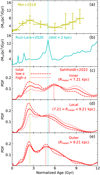 |
Fig. 1 Recently reported episodes of star formation in the late history of the local region of our Galaxy. From top to bottom: (a) SFR obtained from main-sequence stars (Mor et al. 2019), with error bars in age and SFR intensity. (b) The cyan curve represents the SFH in a bubble of radius ∼2 kpc around the Sun (Ruiz-Lara et al. 2020). The three subsequent panels display results for age distribution of stars obtained from Sahlholdt et al. (2022) for (c) the inner, (d) the local and (e) the outer Galactic disc; in those three panels dashed curves correspond to the situation close to the plane and dotted ones away from the plane, with solid curve representing the total (in percentage). The age range of all data is normalised to the time duration of our model (Tmax = 12 Gyr). In (a) and (b), observations are normalised to the present-day local star surface density (38 M⊙ /pc2) with the adopted IMF of Kroupa (2002). The two vertical lines are to guide the eye and correspond to the centroids of the SFB of Mor et al. (2019), of the strongest SFB of Ruiz-Lara et al. (2020) and of the first SFB of Sahlholdt et al. (2022). |
2 Observations
Three different sets of observational data (Mor et al. 2019; Ruiz-Lara et al. 2020; Sahlholdt et al. 2022) were used to guide our modelling of SFBs in this work. In this section we briefly describe their main features and show possible relation in Fig. 1.
2.1 Mor et al. (2019)
The Besançon Galaxy model combined with an approximate Bayesian computation algorithm was used by Mor et al. (2019) to analyse data from the Gaia DR2 catalogue, which they estimated to be complete up to magnitude G=12. They explored a parameter space with 15 dimensions that simultaneously included the initial mass function (IMF) and a non-parametric SFH for the Galactic disc. The SFH displays a decreasing trend at the early age followed by a prominent star formation rate (SFR) enhancement beginning around 5 Gyr ago. This enhancement lasted for about 4 Gyr and reached its maximum ∼2–3 Gyr ago. During that period, about half of the stellar mass currently observed in the solar neighbourhood was formed (Fig. 1, top).
Isern (2019) used Gaia data to construct the luminosity function of massive white dwarfs (0.9 < M/M⊙ < 1.1) in the solar neighbourhood, for distances d < 100 pc. Because the lifetime of their progenitors is very short, the birth times of both parent stars and daughter residues are very close and facilitate the reconstruction of an (effective) SFH. Isern (2019) found that the SFR started growing from zero in the early Galaxy, reached a maximum 6–7 Gyr ago, then declined and started to increase once more ∼5 Gyr ago, reaching another local maximum 2–3 Gyr ago. The local SFH inferred from the analysis of Isern (2019) very much resembles to the one suggested by Mor et al. (2019).
2.2 Ruiz-Lara et al. (2020)
Ruiz-Lara et al. (2020) have provided a detailed SFH of the local MW disc by comparing colour-magnitude diagrams from Gaia DR2 stars within a 2-kpc sphere around the Sun to synthetic ones, computed with the BaSTI stellar evolution library (Hidalgo et al. 2018) and the IMF from Kroupa (2002). The derived SFH shows three short and prominent star forming episodes occurring ∼5.7, 1.9 and 1 Gyr ago and lasting for about 0.8, 0.2 and 0.1 Gyr, respectively (Fig. 1, second from top). According to Ruiz-Lara et al. (2020) these episodes seem to coincide with the reported pericentre passages of the Sagittarius (Sgr) dwarf satellite galaxy, as recovered from its reconstructed orbital history. The colour-magnitude diagram of the Sgr core also revealed three stellar populations corresponding to these epochs (Siegel et al. 2007). These findings suggest that both the Milky Way disc and Sgr may have been affected by their close interactions in the past few Gyr.
2.3 Sahlholdt et al. (2022)
Combining GALAH DR3 and Gaia Early DR3 data on turnoff stars Sahlholdt et al. (2022) established a detailed map of the age–metallicity distribution in the MW, which was then divided into sub-samples by tangential velocity and Galactic position. These sub-samples revealed three phases in the SFH of the MW separated by two transitions at the ages of 10 Gyr and 4–6 Gyr. In the first phase, kinematically hot and high-alpha stars form in the inner disc. In the second phase, the stellar populations gradually become kinematically colder and have a lower [α/Fe] ratio. At this period, stars form with super-solar metallicities in the inner disc and with sub-solar metallicities in the outer regions. Finally, the third phase is related to a recent SFB (see Fig. 1 bottom three panels, for the inner, local, and outer disc, respectively).
Despite the different methods and age estimates used in the three studies, one may notice that the youngest SFB of Sahlholdt et al. (2022) has the same centroid in time as the one of Mor et al. (2019), while the older of the three SFBs of Ruiz-Lara et al. (2020) roughly coincides with the SFBs of Sahlholdt et al. (2022) in the local and outer discs. On the other hand, the duration of the SFBs varies widely between the studies, from a fraction of a Gyr in the case of Ruiz-Lara et al. (2020) to a couple of Gyr in the case of Mor et al. (2019). Finally, in the case of Sahlholdt et al. (2022), it seems that different radial regions experienced the oldest SFB at different times, since it occurred earlier in the inner disc than in the local and outer ones, as sketched by the dotted red vertical lines in the bottom three panels of Fig. 1: there is a time delay of ∼1.5 Gyr between the peaks of SF in the inner and outer regions, separated by ∼2.5 kpc (if peak SF intensities and ages are taken at face value).
In the next section, we present our model, and in Sections 4 and 5, we explore the consequences of introducing SFBs constrained by the observations presented in the previous subsections.
3 Model
Our model is a one-dimensional ‘multi-ring’ model for the MW, with the rings coupled by stellar radial migration. The model is adapted from Kubryk et al. (2015a,b), as updated recently in Prantzos et al. (2023). Here, we summarise the main features of the model and present in detail our simple method of introducing episodes of enhanced star formation.
3.1 Gas infall and star formation
We assumed that the MW disc is gradually built by primordial gas infall in the potential well of a dark matter halo of 1012 M⊙. The formation of the MW disc proceeds ‘inside-out’, with the time scale of gas infall τin =0.5 Gyr in the innermost zones and gradually increasing with radius up to 7.5 Gyr at 21 kpc.
The ‘Kennicutt–Schmidt’ law (Schmidt 1959, 1963; Kennicutt 1998) is widely used to describe the correlation between surface densities of star formation Ψ and gas ΣG :
 (1)
(1)
However, Bigiel et al. (2008), when analyzing data from nearby disc galaxies, found that the SFR is directly connected to the surface density of molecular gas H2 . Also, based on updated observations, Krumholz (2014) have suggested that H2 correlates better with star formation than the atomic gas HI or the total gas surface density. Following these studies, we assumed that the SFR is proportional to H2 surface density. The semi-empirical method of Blitz & Rosolowsky (2006) was adopted to calculate the fraction of molecular gas (see Appendix B in Kubryk et al. 2015a) and we calculated the SFR in the standard model – with no SFB – as:
 (2)
(2)
We adopted the Initial Mass Function (IMF) of Kroupa (2002) with the slope of high mass range equal to 1.3.
3.2 Stellar migration
The disc is divided in concentric rings of radial width ∆R = 0.5 kpc, and stars are allowed to migrate during their evolution. Following Kubryk et al. (2015a), we adopted a statistical prescription to parameterise the epicyclic motion of stars (blurring) and the true variation in their guiding radius (churning) separately. We used a time-dependent radial velocity dispersion σr ∝ τβ to describe blurring with β = 0.25 (Aumer et al. 2016) and we used the method described in Kubryk et al. (2015a) for churning. We note that a recent analysis of the kinematics and orbits of 23 795 turnoff and giant stars from Gaia-DR2 (Beraldo e Silva et al. 2021), has found that in the solar neighbourhood, about half of the old thin disc stars can be classified as migrators, while for the thick disc this migrating fraction could be as high as one-third. We also note that Feltzing et al. (2020) investigated the amount of radial migration in the MW disc, using data for red giant branch stars from APOGEE DR14, parallaxes from Gaia, and stellar ages based on the C and N abundances and results of the models of Minchev et al. (2018), Frankel et al. (2018), Sanders & Binney (2015) and Kubryk et al. (2015a). They found that half of the stars have experienced some sort of radial migration, 10% likely have suffered only from churning, and a modest 5–7% have never experienced either churning or blurring. They also found that their results depend little on the radial abundance profiles of the adopted models, despite the differences among the latter.
Regarding the locally observed two-branch behaviour of [α/Fe] versus metallicity, two classes of evolution have been proposed: secular and episodic. Observations suggest that stars with distinctly different histories (one corresponding to intense early star formation and another occurring more slowly at late times) co-exist locally today. In the episodic case both histories occur locally, but they are separated by more or less long episodes of intense infall and/or paucity in star formation. Radial migration plays little or no role in this scheme. In the secular evolution case, the intense star formation occurs in the inner disc early on at an epoch where few stars are formed in the solar vicinity (because of the inside-out formation of the disc) and some of those early stars are transported locally by radial migration, which plays a key role in that case; see discussion in the introduction section of Prantzos et al. (2023).
3.3 Nucleosynthesis prescriptions
As in Prantzos et al. (2023), we used the metallicity-dependent yields of Cristallo et al. (2015) for low and intermediate mass stars (LIMS), of Limongi & Chieffi (2018) for Massive Stars1, and of Iwamoto et al. (1999) for themonuclear supernovae (SNIa). We included all isotopes from H to U and all relevant nucleosynthesis process and sites. The yields of Limongi & Chieffi (2018) consider mass loss and rotation and we adopted here an initial distribution of rotational velocities (IDROV) from Prantzos et al. (2018, 2020), which was tailored to match several observables. Philcox et al. (2018) found that this prescription provides a better fit to the solar composition than other sets of yields.
3.4 Star formation episodes
Episodes of enhanced star formation may result from a temporary increase of the amount of gas accreted on a galaxy, or of the star formation efficiency after some external perturbation, or from a combination of the two. Here we assumed enhanced star formation efficiency, defined as SFR per unit mass of molecular gas rather than total gas, in view of the adopted SFR in Eq. (2). For the standard model, we assumed that the star formation efficiency keeps the same value all the time (ε=α). In the case of an SFH with episodes of enhanced star formation, we kept the same prescription for infall and we adopted a modified star formation law:
 (3)
(3)
where Ib(R, t) represent episodes of enhanced star formation. We call these episodes ‘star formation bursts’ (SFBs), although their intensity and duration may vary considerably. In the numerical implementation we assumed that a SFB is characterised by a temporal enhancement of the SFR, without any other modification in the code. This would correspond, for example, to a perturbation of the gas by an external agent, such as a nearby small galaxy. If the enhancement is assumed to be due to a temporal increase of the infall rate or to a gas-rich merger, then the effect of the SFB on the chemical composition would be less important, since the enhanced amount of ejected metals would be diluted to a larger amount of (accreted) gas. On the other hand, one may envisage more complex situations, such as the SFB heating the gas and ‘quenching’ star formation for some time. The real situation would undoubtedly be more complicated than the simplified ones explored here. In this work, we consider three types of SFB: local bursts (occurring in some delimited region of galactocentric radius), global bursts (large perturbations occurring simultaneously over the largest part of the disc) and propagated bursts, starting at some place and propagating outwards.
3.4.1 Local star formation burst
In the local SFB case, it occurs in a small range of galactocentric radii and we used a multivariate Gaussian function of time and radius to describe this type of burst
![Mathematical equation: ${I_b}(R,t) = {\gamma _b}\exp \left[ { - {{{{\left( {R - {\mu _R}} \right)}^2}} \over {2\sigma _R^2}} - {{{{\left( {t - {\mu _t}} \right)}^2}} \over {2\sigma _t^2}}} \right]$](/articles/aa/full_html/2025/02/aa52552-24/aa52552-24-eq4.png) (4)
(4)
where γb is used to describe the maximum intensity of the SFB, µt is the time of maximum star formation efficiency, and µR is the radius where maximum star formation efficiency occurs. The term σt is related to the duration of the SFB, and σR describes the radial range affected by the enhanced star formation. Here, for all local bursts (µR = 8 kpc) we adopted a fixed radial extension σR = 1 kpc, and we simply adjusted the temporal extension µt and the maximal intensity γb to reproduce the observations as closely as possible.
3.4.2 Global SFB
To describe a global SFB affecting the whole disc, we adopted for all radial zones the same amplitude of enhanced star formation γb at the same time. This is of course an extreme simplification of the situation since there is no reason why the SF efficiency should be enhanced by the same factor everywhere. However, the star formation still depends on the total amount of local molecular gas (see Eq. (3)). On the other hand, there are no observational data that allowed us to distinguish between local and global SFBs, so we studied here the simplest case. Thus, we simply described the SFB by a Gaussian function in time:
![Mathematical equation: ${I_b}(R,t) = {\gamma _b}\exp \left[ { - {{{{\left( {t - {\mu _t}} \right)}^2}} \over {2\sigma _t^2}}} \right].$](/articles/aa/full_html/2025/02/aa52552-24/aa52552-24-eq5.png) (5)
(5)
We used both assumptions of local SFB and global SFB to simulate the SFHs constrained by Mor et al. (2019) (single local burst or single global burst) and Ruiz-Lara et al. (2020) (three local SFBs or three global SFBs) as we discuss in the next section.
3.4.3 Propagated star formation burst
Motivated by the results of Sahlholdt et al. (2022), we defined a more specific case of propagated SFB. We assumed that the SFB affects delimited radial zones, as the local SFB, but with a time delay depending on radius, thus simulating the episode of star formation propagated across the disc. We therefore defined the propagated SFB by a modified multivariate Gaussian function:
![Mathematical equation: ${I_b}(R,t) = {\gamma _b}\exp \left[ { - {{{{\left( {R - {\mu _R}} \right)}^2}} \over {2\sigma _R^2}} - {{{{\left( {t - {\mu _t} - {t_R}R} \right)}^2}} \over {2\sigma _t^2}}} \right]$](/articles/aa/full_html/2025/02/aa52552-24/aa52552-24-eq6.png) (6)
(6)
where tR is the characteristic time scale (in Gyr/kpc) of radial displacement of the SF episode, i.e. the inverse of the speed of radial displacement. A positive tR implies that the SFB occurred earlier in the inner regions and its peak moved outward.
4 Results
4.1 Star formation
Figure 2 summarises our results for the cases of local and global SFBs. In column A, we display some results of the baseline model, which is essentially the same as the one presented in Prantzos et al. (2023). In the top-left panel (A1), the true SFHs of different radial zones are displayed and colour-coded, for the inner disc (galactocentric radius R < 5 kpc, red), intermediate region (5 < R < 11 kpc, blue) and outer disc (R < 11 kpc, green), while the local SFH at R = 8 is depicted by dashed blue curve. The inside-out formation of the disc can clearly be seen through the early peak of SFR in the inner zones, compared to the practically constant local SFR and the recently increasing SFR of the outer zones.
In the second row, we display the age distribution of local stars as seen today by an observer in the solar cylinder (7 < R < 9 kpc). The youngest stars have mostly formed locally, because there is little time for radial migration to redistribute stars over the disc. As one moves to greater ages, though, an increasing amount of locally formed stars have left and a greater number of stars produced elsewhere have moved into the local volume. This trend is especially true for stars produced in the inner disc, where the true SFR was quite intense early on (see panel A1). As a result, the perceived local SFH is more peaked early on than it was in reality (panel A2). As in Prantzos et al. (2023), we assumed that the old disc (age >9 Gyr) corresponds to the thick disc and the younger disc to the thin disc (age <9 Gyr), but these considerations are not of importance in this study.
The next two columns in Fig. 2 display results for a single SFB, namely a local (Col. B) and a global (Col. C). We adjusted the intensity and duration of the SFB in order to reproduce in both cases the observationnally inferred SF history in the solar neighbourhood by Mor et al. (2019), as shown in the 2nd row (panels B2 and C2, respectively). Finally, the two columns on the right display results for three SFBs, local (Col. D) and global ones (Col. E). We adjusted their intensity in order to reproduce the SFBs inferred for the local discs from the analysis of Ruiz-Lara et al. (2020), as seen in panels D2 and E2, respectively). In all cases, fitting the observationally inferred SFBs is the main constraint of our SFB parametrisation.
Compared to our baseline model, the introduction of late episodes of enhanced star formation, obviously reduces the importance of the oldest stellar population observed locally because a larger fraction of stars is made at later times. It can also be noticed that in order to reproduce the same local SFH, a local SFB has to be more intense than a global one. The reason is that the latter involves more radial zones and thus produces more stars of a given age that migrate and are found in the solar neighbourhood today.
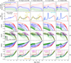 |
Fig. 2 Comparison of various quantities as function of age among models with five different SFHs (standard, single local SFB, single global SFB, three local SFBs, and three global SFBs). Row 1: true SFR in different radial zones, divided into inner disc (R < 5 kpc, red), intermediate disc (5 < R < 11 kpc, blue) and outer disc (R > 11 kpc, green). The evolution at R⊙ = 8 kpc is depicted by dashed blue curve. Row 2: SFH as observed today in the solar cylinder (7 < R < 9 kpc) after counting stellar radial migration. The vertical dotted line at 9 Gyr separates the disc (age >9 Gyr, red) from the disc (age <9 Gyr, blue). Row 3: evolution of [Fe/H] in the gas in different radial zones. Thick portions of curves indicate the periods of SFR higher than the time-averaged one. Row 4: [Fe/H] of stars existing in solar cylinder at the end of the simulation. The colour-coded filled contours represent the number density of stars. As shown on the left colour bar, the contour levels correspond to the fractions of 0.001, 0.1, 0.3, 0.5, 0.7, 0.9 of the total numbers of stars. The red and blue curves indicate the average [Fe/H] of the thin and thick discs. Row 5: evolution of [Si/Fe] in the gas in different radial zones. Row 6: [Si/Fe] in stars found in the solar cylinder at the end of the simulation. The fraction of young α-enhanced stars selected using the criterion from Chiappini et al. (2014) (magenta) and Zhang et al. (2021) (brown) are shown on the top left, along with the corresponding fractions of stars in those regions as obtained by our models (see text). Orange dots denote young, high [α/Fe] stars from Miglio et al. (2021). |
4.2 Abundances versus age
The two subsequent rows of Fig. 2 describe the evolution of metallicity in the gas of all the zones (Row 3) and in the stars now present in the solar vicinity (Row 4). Thick parts of the curves in Row 3 correspond more active periods, when the SFR in each zone is higher than the corresponding time- averaged value. These results have been analysed in detail in Prantzos et al. (2023). We note that in the baseline model, the Sun is found to be formed a couple of kiloparsecs inwards from its present position, at a galactocentric distance R∼6 kpc. This brings in agreement the fact that the solar metallicity is very close to the one of local young stars (Nieva & Przybilla 2012) and the ISM (Cartledge et al. 2006; Ritchey et al. 2023), while models suggest a sizeable metallicity evolution in the local gas in the past few Gyr (e.g. Minchev et al. 2013; Kubryk et al. 2015a; Prantzos et al. 2018, 2023).
When moving to the right in Row 3 of Fig. 2, we find that the single SFB that was adjusted to reproduce the SFH of Mor et al. (2019), drives a strong increase of the late metallicity after the Sun’s formation (panels B3 and C3) since the peak of the SF efficiency is located at ∼2.5 Gyr in the past. Two factors contribute to that increase: (a) the enhanced rate of SNIa – the main Fe producer – a few hundred Myr after the SFB and (b) the small amount of gas left after the intense SFB. The combined result of (a) and (b) is that a large amount of Fe is released in a small amount of gas, rapidly increasing its metallicity. We also note that this late metallicity increase is more pronounced in the case of a local burst (panel B4) than in a global one (panel C4). The reason, as explained also in the last paragraph of the previous section, is that the local burst has to be more intense than the global one to reproduce the same current stellar density in the solar vicinit. As a result, it increases the local gas metallicity more. On the other hand, the first of the three SFBs inferred by Ruiz-Lara et al. (2020) as occuring 6 Gyr ago lasts much less time than the one of Mor et al. (2019) and produces a steeper increase in [Fe/H] (panels D3 and E3 in Fig. 5).
Our results for the impact of an SFB on the age–metallicity relation differ from the ones presented by Johnson et al. (2021). They find that [Fe/H] is considerably reduced during the SFB, because they assumed that the SGB is fuelled by an intense infall that dilutes metallicity. We assumed instead that the SFBs are due to perturbations induced by close-by interactions with other galaxies and thus the metallicity in all radial zones of the disc never decreases in the models presented here. We also tested cases with enhanced infall and found similar dilution effects, but only in the case of local SFBs (see Sect. 7).
4.2.1 Impact on the Sun’s birthplace
The strong late metallicity evolution induced by the recent SFB has an important impact on the determination of the birth radius of the Sun. Since the present-day metallicity of the local gas must be near solar2, its difference with the local gas metallicity 4.5 Gyr ago is much smaller in the baseline model (∼0.25 dex) than in the SFB scenario B or C (local or global SFB, respectively). For that reason, the Sun’s birthplace in that case is in a region further inwards than in the baseline model, around R∼4.5–5 kpc. The exact values of course depend on the adopted model and radial migration scheme. However, the key point is that a late SFB (after the Sun’s formation) ‘pushes’ the birth position of the Sun further inwards, more than a recent smooth SFH.
The situation is slightly different in the case of an SFB prior to the formation of the Sun, as illustrated in panel D3 and E3 of Fig. 2, obtained for the SFH of Ruiz-Lara et al. (2020). The oldest and strongest of the three SFBs occurs just prior to the formation of the Sun, abruptly increasing the gas metallicity. After that, star formation activity becomes low (because little gas is left) and metallicity increases very little, since the two most recent SFBs of Ruiz-Lara et al. (2020) are not strong enough to change that situation. As a result, the final local gas metallicity is only ∼0.15 dex higher than its was 4.5 Gyr ago at R ∼ 8 kpc. In contrast to the previous case (i.e. an SFB after the Sun’s birth), the abundance gradient in the intermediate disc is now small, as can be seen by the density of the blue curves at the age ∼4.5 Gyr in panel D3 and E3. Despite this small metallicity difference, we note that the birthplace of the Sun suggested by the model is still at R∼5–5.5 kpc, which is slightly smaller than in the baseline model.
Thus, we find that a strong SFB may play an important role in the determination of the Sun’s birthplace. It may increase or decrease the absolute value of the abundance gradient (depending on whether it occurs after or before the Sun’s formation, respectively), but it always places the Sun’s birth radius further in the inner disc than in the baseline model with no SFB.
We note that Lu et al. (2024a) find a low value for the birth radius of the Sun of R⊙,b = 4.5±0.4 kpc, which substantially lower than most other studies, including this one. In their Fig. 6 (top right panel), they display the age–metallicity relations at birth radii, showing a rapid metallicity increase in most radii at approximately the time of the Sun’s formation, similar to the features displayed in the third row of our Fig. 2.
4.2.2 Overdensities in the plane of abundances vs age
The fourth row of Fig. 2 displays the age-[Fe/H] distribution of stars found today in the solar cylinder. The scatter of [Fe/H] at a given age results from stars born in different radial zones with different chemical evolutions, as already found in the pioneering paper of Sellwood & Binney (2002). In our standard model (panel A4), there are two overdense regions that correspond to a young (a few Gyr) and an old (more than 9 Gyr) stellar population, which are identified to the thin and thick discs. Most stars in the old overdensity are formed early in the inner region and their [Fe/H] increases very rapidly with time. The young overdensity represent stars formed mostly locally, with [Fe/H] ∼ 0 and increasing little with time.
In that same panel A4 of the figure, we overplot the data of Nissen et al. (2020), who used HARPS spectra to determine metallicities (in the range of −0.3 < [Fe/H] < +0.3) for 72 nearby solar-type stars and ages by adopting ASTEC stellar models and Gaia DR2 parallaxes. They found that their sample is rather clearly split in two sequences: a sequence of old stars with a steep rise of [Fe/H] to +0.3 dex at an age of ∼7 Gyr and a younger sequence with [Fe/H] increasing from about −0.3 dex to +0.2 dex over the past 6 Gyr. They interpreted this split as evidence of two episodes of accretion of gas onto the Galactic disc with a quenching of star formation in between. We find that in our standard model this trend is naturally explained, as can be seen in panel A4 and also explained in detail in Prantzos et al. (2023, see Fig. 4 in that work). The reason is that, in the framework of that model, stars in the inner disc (which is older because of the inside-out formation scheme) are produced abundantly and metallicity rises rapidly in the early stages. In contrast, in the local disc metallicity rises slowly and later. Radial migration brings in the solar vicinity stars from the inner disc and thus two branches (overdensities) are obtained. Nissen et al. (2020) interpreted their finding in terms of the two-infall model, in which all the action takes place in the same environment: a one-zone model with a unique but discontinuous history that has two distinct epochs of star formation separated by a hiatus or quenching. In contrast, in multi-zone models with radial migration, the early intense phase of stellar activity occurs in the inner disc and the late phase mostly occurs locally.
In the fourth row of Fig. 2, the single late burst models (local or global) preserve the positions of these two populations while enhancing the density of the young population with respect to the standard model (panels B4 and C4, to be compared to A4). On the other hand, the three local SFBs model (panels D4 and E4) create three small and narrow overdensities. The first of the three local SFBs (5 Gyr ago) creates a small decrease in the average [Fe/H] versus age relation of the stars found today in the solar cylinder, for ages between 4 and 5 Gyr. This ‘depression’ is due to a complex interplay between the star formation activity of the inner Fe-rich zones prior to the SFB (with some of their stars having migrated to R=8 kpc) and the fact that just after the burst, the local ISM is enriched in Fe only by the core collapse supernovae (CCSNN) of the massive stars, while a few hundreds of Myr later the SNIa of the SFB produce a rapid increase of the Fe abundance. Unsurprisingly, this feature is absent in the case of the global burst (panel E4).
This peculiar feature of an SFB (the delayed overproduction of Fe from SNIa with respect to the α-elements that are produced exclusively by CCSN) is also reflected in another observable, namely, the behaviour of [α/Fe] versus [Fe/H], as can be seen in the next two rows of Fig. 2. In the fifth row we show the evolution of [Si/Fe], using Si as a representative α element. The ratio of CCSN to SNIa decreases with time everywhere; however, the decrease occurs more strongly in the inner disc where the SFR decreases very rapidly after the first couple of Gyr and much less in the outer disc where the SFR remains important untill today (see first row in Fig. 2). As a result, in the standard model (panel A5), the [Si/Fe] of the gaseous disc decreases steadily and more rapidly in the inner disc than in the outer one at early times. Also in that model, the [Si/Fe] of local stars today (panel A6) decreases rapidly in the earliest times (since most of the oldest local stars have migrated from the inner disc) and then very little (since the youngest stars are formed mostly locally).
These features are also encountered in the other columns of the last row of Fig. 2, but the introduction of SFBs produces different overdensities in the phase space at the epochs of the SF efficiencies. Those overdensities appear at the age of starburst but in general produce higher [α/Fe] values than those of the standard model. This is clearly seen for the local bursts of panels B6 and D6, respectively, where the post-SFB [α/Fe] rises by 0.1 dex and 0.3 dex, respectively. We explore the implication of that effect concerning the issue of young and high [α/Fe] stars in the next sub-section.
4.2.3 Young [α/Fe] -rich stars?
In the case of a broad SFB 3 Gyr ago (as the one claimed in Mor et al. 2019), whether local or global (panels B6 and C6 of Fig. 2), the decline of Si/Fe is stopped for some time after the SFB, because of the enhanced Si/Fe contributed by CCSN. Later, however, because of the Fe injected by the SNIa of the SFB, the Si/Fe decreases rapidly, as can be seen for the stars formed in the past 2 Gyr. Thus, a single late SFB is expected to leave a clear, albeit weak, signature of a late decrease in the [α/Fe] versus [FeH] relation.
A stronger signature is obtained in the case of a strong and narrow SFB, such as the first of the three SFBs of Ruiz-Lara et al. (2020), as displayed in the panels D6 and E6 of Fig. 2. This time, an important temporary increase, by ∼0.3 dex, is obtained in the [Si/Fe] ratio right after the first burst 5 Gyr ago and for a short period because that SFB has a shorter duration than the one of Mor et al. (2019).
Thus, a generic feature of narrow SFBs, independent of their time of occurrence, is a temporal enhancement of the [α/Fe] ratio, which is obtained for a short time and immediately after the SFB. This confirms the original intuitive work of Gilmore & Wyse (1991), the recent analytical findings of Weinberg et al. (2017) and the numerical findings by Johnson & Weinberg (2020), albeit only qualitatively. The amplitude of the SFBs considered in those works is smaller than what is used here, and consequently the enhancement of [O/Fe] is also smaller.
Johnson et al. (2021) and Borisov et al. (2022) note that this feature may be of interest regarding the population of the ‘young [α/Fe]-enhanced’ stars reported a few years ago with data from APOGEE (Chiappini et al. 2015 and Martig et al. 2015). Those stars are younger than 5–6 Gyr and designated as thin disc stars, while their [α/Fe] ratio is around 0.2 dex higher than in typical thin disc stars and closer to those of the thick disc. Jofré et al. (2016) suggested that the properties of those stars may be explained by mass transfer in close binaries, but Anders et al. (2017) noticed that this hypothesis cannot explain the different number counts in the inner and outer disc.
Zhang et al. (2021) with LAMOST data and Miglio et al. (2021) using CorroAPOGEE data argued that the higher than average masses of the aforementioned stars favour the interac- tion/merger hypothesis, which would make old and [α/Fe] -rich stars – normally encountered in the thick disc – appear younger. These conclusions are supported by recent chemical and kinematic studies of Queiroz et al. (2023), Cerqui et al. (2023), and Grisoni et al. (2024) who find that these stars display similar kinematic properties with those of the high-α disc. We note, however, that Borisov et al. (2022) reach different conclusions using GALAH data: they find that their sample of ‘young [α/Fe]- enhanced’ dwarf stars exhibits lithium abundances similar to those of young [α/Fe]-normal dwarfs at the same age and [Fe/H].
Here, we quantitavely investigate whether a recent SFB induced by enhanced star formation efficiency, without any additional infall of high-α gas, could create a population of young [α/Fe]-enhanced stars. The boxes delimited by the two orthogonal (brown) or quasi-orthogonal (magenta) lines in the panels of the sixth row of Fig. 2 correspond to the regions that should not contain stars, i.e. relatively young and with high [α/Fe] , according to Zhang et al. (2021) and Chiappini et al. (2014), respectively (the young alpha-rich stars from the K2 survey in Grisoni et al. (2024) are also contained within the ‘forbidden’ region of the latter reference). Moreover, we plot in those figures the 25 ‘overmassive’ stars (orange points) with high [α/Fe] reported in Miglio et al. (2021). The percentages reported inside those boxes display the fractions of our model stars found in the corresponding regions. It can be seen that in our standard model, a few percent of our stars are found in the ‘forbidden’ region of Chiappini et al. (2014), but less than 1% are in the more restricted zone of Zhang et al. (2021).
The introduction of SFBs, in particular the oldest of the three of Ruiz-Lara et al. (2020) (panel D6 of Fig. 2) increases considerably the aforementioned fractions, but the youngest stars with the highest [α/Fe] remain inaccessible to our modelling. The reason is that at such late times, the average [α/Fe] in the local and nearby inner disc (the stars of which have time to radially migrate to the solar neighbourhood) is quite low and the small recent SFBs of Ruiz-Lara et al. (2020) or the strong and extended one of Mor et al. (2019) cannot increase it to the level required by the data (i.e. [α/Fe] > 0.20). A couple of recent (age <3 Gyr) strong and short SFBs – such as the oldest one in Ruiz-Lara et al. (2020) – could help in that respect, but such events have not been reported. Another possibility could be a ‘top-heavy’ IMF during the SFB, increasing the [α/Fe] to much larger extent (say 0.3 or 0.45 dex) than the conventional IMF adopted here. We do not attempt to model such events in this work. We simply note that in those cases, the kinematic properties of those young and [α/Fe] -rich stars – resembling those of the thick disc, as noticed by Queiroz et al. (2023) and Cerqui et al. (2023) – could be readily explained by the highly turbulent environment inherent to an SFB.
4.3 Properties versus metallicity
In Fig. 3, we present the results of our models as function of metallicity and compare to observational data.
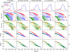 |
Fig. 3 Model results (colour coded as in Fig. 2) and comparison to observations for various quantities as function of [Fe/H], Row 1: metallicity distributions for thin (blue) and thick (red) discs in the solar cylinder. The thin ones are compared to the red giants near the plane (|ɀ| < 0.3 kpc) from the APOGEE DR17 (dotted grey). Row 2: age-metallicity relation for all radial zones. Row 3: predicted age versus [Fe/H] distribution present in the solar cylinder. The average ages of thin and thick discs (red and blue curves) are compared to data from Feuillet et al. (2019) shown by orange curves with vertical error bars. Row 4: gas evolution of the various radial zones of the model in the [Si/Fe]-[Fe/H] plane. Row 5: predicted [Si/Fe] versus [Fe/Hl distribution present in solar cylinder. |
4.3.1 Metallicity distributions
In the top row we display the metallicity distribution (MD) and compare to data for the thin disc (dotted) taken from APOGEE DR17 (Abdurro’uf et al. 2022). Following Hayden et al. (2015), we applied the following restriction and quality criteria to APOGEE DR17: 1.0 ≤ log ɡ ≤ 3.8, 3500 ≤ Teff ≤ 5500 K, SNR < 80, ASPCAP flag ∉ STAR_BAD or VSINI_WARN.
Using distances from Gaia EDR 3 (Bailer-Jones et al. 2021), we limited the radial Galactocentric distance to the range 7 < R < 9 kpc and distance from the plane to |ɀ| < 0.3 kpc to get a sample of mostly thin-disc stars in the solar cylinder. Our model results are plotted as solid curves for the thin (blue) and thick (red) discs.
In our standard model, the MD of thin disc (panel A1) peaks at [Fe/H] ~ 0 and compares fairly well with the APOGEE sample except for a slightly extended tail to the lower metallicities. The introduction of SFBs pushes the peak metallicity of the MD to lower values and broadens it significantly (subsequent panels in first row). The largest dispersion of the MD is due to the fact that a large fraction of the stars is made during, or shortly after, the SFBs, when the Fe abundance increases substantially. In the extreme case of three local SFB, the first burst 6 Gyr ago triggers a secondary peak at [Fe/H] ~ −0.3 dex (panel Dl). It is worth noting that such a double-peaked distribution, at approximately the same metallicity values, has been found in the APOGEE DR17 data in the range 7–9 kpc evaluated at stellar birth radii, as reported in Fig. 4 of Spitoni et al. (2024). In that same figure, the [Si/Fe] versus [Fe/H] diagram displays two overdensities at approximately the same positions as in panel D5 of our Fig. 3. Taking into account the uncertainties in stellar ages and the evaluation of stellar birth radii (see Sect. 6), as well as those in our radial migration model, we consider the above as an interesting but inconclusive finding.
To summarise this section, we find that the local MDs may be considerably affected by the introduction of recent SFBs and may be used as a constraint regarding the SFB intensity and perhaps other properties (e.g. their extent in space and time). However, a detailed investigation of those effects is beyond the scope of this study.
4.3.2 Age versus metallicity
In the second row of Fig. 3, we display age versus metallicity results for the gas in all radial zones and in the third row we show the situation for stars present today in the solar cylinder. We compare them with the corresponding data from SDSS and APOGEE obtained in Feuillet et al. (2019). We used their results in the zone limited by 7<R<9 kpc and 0<|Z|<0.5 kpc. The behaviour of the average age in the data could be divided into four phases strongly correlated with radial migration as discussed in Kubryk et al. (2015a) and Prantzos et al. (2023). Obviously, the first phase of the lowest [Fe/H] and highest [α/Fe] corresponds to stars older than 9 Gyr, which belong to the thick disc in our models. The relative paucity of stars with ages between 9 and 6 Gyr is similar to the corresponding panel A4 of Fig. 2 and it is discussed extensively in Prantzos et al. (2023).
After this transition, the average age decreases slowly with metallicity up to about solar [Fe/H] i.e. the present-day metallicity of the local gas and young stars. The subsequent rising of the curve, both in the model (panel A3) and the data of Feuillet et al. (2019), is attibuted to the fact that local supersolar metallicity stars originate in the inner disc of higher metallicity, and they need more time on average to radially migrate to the solar neighbourhood (Kubryk et al. 2015a; Prantzos et al. 2023). The last downturn to lower ages observed for the highest metallicities is attributed to a small number of relatively young stars (~3 Gyr old) formed at galactocentric distances of RG ~2 kpc where the metallicity is ~0.4–0.5 dex. Those stars migrated rather rapidly to the solar vicinity, at an average speed of ~2 kpc/Gyr, compared to the typical average speed of ~ 1 kpc/Gyr.
Considering the relatively large errors in age determination, our standard model presents a fairly good agreement with observational data. On the other hand, all the models with SFBs preserve the ‘down-up-down’ feature of the relation of average age with metallicity, but the local SFBs make the corresponding slopes steeper (shallower) for local (global) SFBs. Also, local SFBs reduce the minimum average age (around solar [Fe/H] by about one Gyr. In any case, the current uncertainties in age determination make it difficult to conclude anything on the basis of existing observations.
4.3.3 [α/Fe] versus [Fe/H]
In the fourth row of Fig. 3, we show the relation of [Si/Fe] versus [Fe/H] for the gas in all the zones. For the standard case, the evolution is smooth and there is no overlap among the evolutionary tracks of the various zones. In the two scenarios of local SFBs, the tracks of the intermediate zones (blue) overlap strongly, due to the significant increase of their [Si/Fe] with increasing [Fe/H]. In those zones, [Si/Fe] reaches a local maximum near the peak of star formation and then plunges to a nearly normal level as the Fe of the delayed SNIa of the SFB catches up to the excess O released earlier by the CCSN of the SFB. The tracks of zones affected by the local SFBs cross largely with those of inward zones (panels B4 and especially D4). Models with global SFBs display similar but less pronounced trends in the fourth row.
The bottom row of Fig. 3 compares our predictions in the plane of [Si/Fe] versus [Fe/H] for the solar cylinder. The two sequences of high [α/Fe] and low [α/Fe] are clearly distinguished in the standard scenario (panel A5), and respectively correspond to the thick and thin discs. As discussed extensively in Prantzos et al. (2023), secular evolution can produce such double-branch behaviour, which is due to the inside-out formation of the disc combined with radial stellar migration and different evolving time scales for the α elements (originating from short-lived CCSN) and for Fe (from SNIa with long-lived progenitors). Very few old stars are formed in the local disc (because of the assumed inside-out formation), thus the locally observed old (and [α/Fe] rich) population is brought into this region by radial migration from the inner disc.
This idea is in line with the conclusions of Buck (2020) who used hydrodynamical plus N-body simulations to find that the local high-[α/Fe] sequence is due to stars formed in the inner disc while the local low-[α/Fe] sequence corresponds to stars formed over the whole disc; in both cases, those stars have been distributed across the disc through radial migration. In fact, the model of Buck (2020) is a kind of ‘hybrid’ model requiring radial migration to bring locally inner disc stars for the high-alpha sequence and a ‘wet’ merger several Gyr ago in order to dilute the metallicity of the interstellar medium and reproduce the low-alpha sequence. In our model, the high-alpha sequence is obtained in a similar way, but the low-alpha one is naturally obtained by the slow local evolution. The model of Buck (2020) apparently implies that without a merger there would only exist the high-alpha sequence in the solar vicinity.
The introduction of SFBs modifies that scheme by enhancing the young population (as already discussed in the previous section) and consequently enhancing the low-[α/Fe] sequence at the expense of the high-[α/Fe] one. However, the double-branch behaviour of [α/Fe] versus [Fe/H] is preserved, in general, with the exception of the case of panel D5, where the older and strongest of the two SFBs of Ruiz-Lara et al. (2020) creates an overdensity that bridges the gap between the high- and low-[α/Fe] sequences because of the ‘crossing’ of the tracks obtained in panel D4.
In summary, the introduction of SFBs into our baseline models perturbs the double-branch behaviour of the local [α/Fe] versus [Fe/H] relation by (a) weakening the high [α/Fe] branch and (b) making the two branches join in the case of a strong and short SFB – as occurs with the oldest one of the Ruiz-Lara et al. (2020) study (panel D5 of Fig. 3).
5 Propagated star formation burst
In order to reproduce the observations of Sahlholdt et al. (2022), which concern not only the local disc but also the inner and outer ones (see the three lower panels of Fig. 1) we adjusted the parameters of Eq. (6). We adopted two SFBs. The older SFB is described with a centre radius µR = 5.5 kpc and propagates more slowly outwards tR = 0.42 Gyr/kpc, while the younger one is cen-treed on µR = 7 kpc and propagates faster, with tR = 0.16 Gyr/kpc. The second SFB is weaker and affects a smaller radial range. In the top-left panel of Fig. 4, we display the true SFHs of all the radial zones of the model, showing the two propagated SFBs.
As shown in the top-right panel of Fig. 4, this arrangement allowed us to roughly reproduce the age distributions of the inner, local and outer sub-samples from Sahlholdt et al. (2022). Our propagated SFB scheme allowed us to reproduce the different times of the older SFB peaks observed in the various zones, as indicated in the figure. Although the positions and intensities of both SFBs are rather well reproduced, the earliest parts of the number distributions of stars in all zones seem to be overproduced, but this is most probably due to the magnitude-limited sample adopted in Sahlholdt et al. (2022), which disfavours older objects.
The bottom rows of Fig. 4 display the age-metallicity relation of our propagated model. On the left we show that relation in the gas for all the zones of the model. As already seen in the previous sections, the introduction of SFBs soon after produces a sudden increase of metallicity in the affected zones, with Fe released initially from CCSN and on longer time scales from SNIa. We show in the next section how this behaviour may affect the evolution of radial abundance gradients.
In the bottom-right panels of Fig. 4, we display the isocontours of the number densities of stars currently found in the three radial zones (inner, local, and outer) in the age-metallicity plane. We superpose the half-maximum contour curves for stars of high-ɀmax (dotted) and low-ɀmax (dashed) from Sahlholdt et al. (2022). We used the same recipe as Sahlholdt et al. (2022) – adapted from Salaris et al. (1993) – to define the metallicity M/H as
![Mathematical equation: $[{\rm{M}}/{\rm{H}}] = [{\rm{Fe}}/{\rm{H}}] + \log \left( {0.638 \times {{10}^{[\alpha /{\rm{Fe}}]}} + 0.362} \right)$](/articles/aa/full_html/2025/02/aa52552-24/aa52552-24-eq7.png) (7)
(7)
and we used Si as proxy for α elements in order to calculate the model [α/Fe].
We find that the overdensities obtained in our model correspond fairly well to those of Sahlholdt et al. (2022), both in metallicity and age, especially if one takes into account the uncertainties in the evaluation of the latter. In the inner disc (5–7 kpc), the intermediate age population (corresponding to the older SFB) is connected to the late thick disc stars and shares almost the same average metallicity with the younger SFB, around [Fe/H]=+0.2. In the local disc (7–9 kpc), the average [M/H] of two corresponding populations decreases from ~0.2 to near solar – again in excellent agreement with the data – and there is no connection to the thick disc population. Finally, in the outer disc, there are still two overdensities, but only the younger one has the correct age and metallicity, while the older one is less metallic by ~0.2 dex compared to the Sahlholdt et al. (2022) results. Overall, our propagated SFB model manages to reproduce the position of the two overdensities in the age–metallicity plane, as derived from those observations, in both the inner and local disc, but it fails to reproduce the older one in the outer disc.
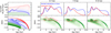 |
Fig. 4 Results of the propagated SFB model. Left: same as the second and fourth row of Fig. 2, for the evolution of SFR and [M/H], Right: age distributions are displayed in the top panel for different radial ranges of 6–7, 7–9 and 9–10 kpc, corresponding to the equivalent observational sub-samples in inner, local, and outer bins shown in Fig. 6 of Sahlholdt et al. (2022); observations (red curves) are compared to model results (blue curves). In the lower panels, age–metallicity relations of the model (green isodensity contours) are compared to half-maximum density contours from observations of Sahlholdt et al. (2022) (dotted and dashed red curves indicate the high-ɀmax and low-ɀmax part of observations in each radial range). |
6 SFBs and the evolution of the metallicity gradient at birth radii
In this section, we discuss the impact of SFBs on the abundance profile of the Galactic disc, and on the possibility of the ‘reconstruction’ of its past evolution through local observations.
The evolution of the abundance profile plays a key role in our understanding of the MW disc. Most studies predict a flattening of the abundance profile of the disc gas with time as a natural result of the inside-out formation of the disc (e.g. Ferrini et al. 1994; Boissier & Prantzos 1999; Hou et al. 2000; Fu et al. 2009; Kobayashi & Nakasato 2011; Pilkington et al. 2012; Gibson et al. 2013; Kubryk et al. 2015a; Mollá et al. 2017; Tissera et al. 2017; Mollá et al. 2019), while others predict the opposite effect (e.g. Diaz & Tosi 1984; Chiappini et al. 1997; Schönrich & Binney 2009; Mott et al. 2013; Grisoni et al. 2018; Vincenzo & Kobayashi 2020) due to, for example, the assumption that the whole early disc was rapidly formed and fully mixed or to late dilution of the outer disc with metal poor gas from mergers.
If stars maintained their radial position at birth during galactic evolution, then good knowledge of their ages and their galactocentric distances would allow one to reconstruct the evolution of the gaseous abundance profile. For many years, objects covering a substantial age range (several Gyr) and bright enough to be seen in a broad range of galactocentric distances, such as planetary nebulae and open clusters, were used to monitor the evolution of the Galactic abundance gradient (e.g. Maciel et al. 2006, 2007; Magrini et al. 2017, 2023, and references therein).
However, as noticed in such works as Minchev et al. (2013, 2018); Kubryk et al. (2015b) the stellar abundance profile of the disc is strongly altered by radial migration (see e.g. Fig. 6 of Kubryk et al. 2015b). This idea has now been confirmed (see Anders et al. 2023), and makes tracing back the evolution of the true abundance gradient in the gas of the disc (difficult that is, at the birth radii of stars observed today).
Based on an idea of Minchev et al. (2018), Lu et al. (2024a) recently attempted to solve that problem. They explored the results of different suites of cosmological hydrodynamical simulations of MW-like galaxies from Lu et al. (2022) who found a tight anticorrelation between the ISM gradient ∇[Fe/H] (in dex/kpc) at a certain look-back time and the locally observed 5% to 95% percentile range of metallicities Δ[Fe/H] (in dex) of the sample stars with the corresponding age. Lu et al. (2024a) applied this finding to a sample of ~80000 sub-giant stars of LAMOST DR7 presently located in the galactocentric distance range RG=6 to 12 kpc, with an average age and metallicity uncertainty as small as 0.32 Gyr and 0.03 dex, respectively. They adopted a present-day value of −0.07 dex/kpc for the present-day gradient and they inferred the value of the central disc metallicity [Fe/H](Rb=0) from the upper envelope of the observed age-metallicity relation. Then they fixed the coefficient of the linearity between the range A [Fe/H] and the gradient at −0.15 dex/kpc because this value allowed them to better reproduce the statistics (guiding radius distribution) of their local stellar sample. Thus, they found a steepening of the [Fe/H] gradient at the birth radius with age, up to 8–9 Gyr ago; at that time, the trend is inversed, and the abundance profile flattens at the oldest ages. The authors associated this inversion to the last major merger, namely the Gaia Sausage/Enceladus event (Belokurov et al. 2018; Helmi et al. 2018).
More recently, Ratcliffe et al. (2023) followed a similar method as Lu et al. (2024a) and recovered the metallicity gradient based on ~140000 APOGEE DR17 red giant disc stars combined with ages from Anders et al. (2023). They found a similar trend as Lu et al. (2024a), but with two additional fluctuations in the temporal behaviour of the gradient, which they attributed to recent SFBs, since the fluctuations occur at approximately the times of passages of the Sagittarius dwarf galaxy.
In a previous work (Prantzos et al. 2023), we explored the idea of Lu et al. (2024a) in order to infer the evolution of the stellar abundance gradient at birth radius in the model of the MW from present-day observations of the age and metallicity of local stars. We showed that a qualitatively similar behaviour as in Lu et al. (2024a) can be obtained, albeit for different reasons. We present the method below, in more detail than in Prantzos et al. (2023), and then we discuss our results for the baseline (no SFB) model and with SFBs.
6.1 The method
In Figs. 5 and 6, we present our method step by step in detail. Figure 5 shows the results as function of age and Fig. 6 as function of birth radius Rb. The latter figure explicates some of the steps undertaken in the former and we move back and forth between the two during the presentation of the method. In both figures, the left column (A) displays our standard model (without SFBs) and the right column (B) shows the model with two SFBs. The former model is compared to the results of Lu et al. (2024a), as already done in Prantzos et al. (2023) while the latter is compared to the results of Ratcliffe et al. (2023). In model (B) with SFBs, the epochs of the two star formation episodes (at 4.5 and 7 Gyr) are indicated with vertical dotted lines through all the panels.
In the top panels of Fig. 5, the evolution of [Fe/H] in the gas of various zones is displayed and has the same colour coding as in Fig. 2. In model (B) on the right, the SFB results in a sharp increase of metallicity in several zones. In panels A2 and B2 of Fig. 5 we show the age–metallicity relation of stars presently found in the solar vicinity, compared to the isodensity contours found in the local APOGEE sample by Anders et al. (2023). Our model (B) reproduces the overdensity at ~4.5 Gyr found in that work and creates a more metal-poor overdensity at ~7 Gyr, because we kept the radial positions of the two SFBs the same as in the propagated SFB model of the previous section but we adjusted their temporal positions according to the Anders et al. (2023) data.
In panels A3 and B3 we display the same local age-metallicity relation, delimited by either the ± σ limits (orange shaded area) or the 95%tiles (two blue dotted curves). The former limits have been used in the works of Lu et al. (2024a) and Prantzos et al. (2023) and we adopted them here for consistency with our previous work, while the latter were adopted in Ratcliffe et al. (2023) and we compare our model (B) with that work in the right column. In all of these cases, it is clear that at late times the range of local stellar metallicities is small (because of the little time available for radial migration). It increases with age because there is more time available for radial migration and then becomes narrow again because the older local stars are formed in the inner disc, which has evolved on a short time scale with high star formation efficiency and in a highly turbulent environment as assumed in our model, resulting in fairly similar early age-metallicity trajectories. The same behaviour is generally obtained in panel B3, but its delimiting curves display a ‘wiggly’ behaviour, with their width temporally compressed during each episode of enhanced star formation.
In panels A4 and B4, the behaviour of the metallicity range Δ[Fe/H] = [Fe/H]max(τ) − [Fe/H]min(τ), analysed in the previous paragraph, appears respectively as solid curves for our models (blue for the 95%-tile limits and orange for the 1σ limits) and as dashed curves for the observational-based inferences of Lu et al. (2024a) (magenta dashed on panel A4) or Ratcliffe et al. (2023) (red dashed on panel B4). All the curves first increase with age, then go through a maximum around 8–9 Gyr and decrease again, for the reasons exposed in the previous paragraph.
Up to this point (the fourth rows in Fig. 5), our method exactly follows that of Lu et al. (2024a) and Ratcliffe et al. (2023), providing the metallicity range Δ[Fe/H] of stars observed locally as a function of age. However, our approach diverges hereon because we know the gas metallicity profiles (i.e. at the birth radius of the locally observed stars) in our model throughout the Galactic history, while Lu et al. (2024a) and Ratcliffe et al. (2023) had to infer them, making a couple of assumptions, as discussed above. One of their main assumptions (to be discussed below) is that the metallicity profile is characterised at any time by a unique slope over the whole radial range.
In our case, the evolution of the abundance gradient at the birthplace inferred through a sample of stars presently found in the solar vicinity is obtained using a slightly different method than that of Prantzos et al. (2023). The method is illustrated in Fig. 6, again for the standard model (left column) and the two-SFB model (right column). In the top panels of Fig. 6, we present the distributions of birth radii Rb for stars currently present locally (i.e. within the grey shaded area), colour-coded as a function of stellar ages (with 1 Gyr age bins). It can be seen that the older stars currently present in the solar vicinity, were mostly formed in the inner disc. The distributions of birth radii move towards solar vicinity with time because younger stars have less time to migrate. In panel Bl of Fig. 5 it can be seen that the introduction of SFBs modifies the birthplace distributions at intermediate ages.
In panels A2 and B2, we display the gaseous metallicity profiles of the Galactic disc for a given age bin (1 Gyr wide), colour-coded as indicated in panel A1. The two blue dotted curves delimit the Rb range corresponding to the 95% tiles of the metallicity ranges of local stars at each age bin, as shown in panels A3 and B3 of Fig. 5. One can immediately see that the gas profile inside the region ΔRb between those two delimiting radii indeed has a single-slope at late times but not at early times since the early metallicity profiles in the inner disc are flat (following our assumption of an early period of very rapid star formation and highly turbulent gas). This indicates that the assumption made by Lu et al. (2024a) and Ratcliffe et al. (2023) (a single slope of the metallicity profile over the whole radial range at any given time) is not applicable, at least in the case of our model. Moreover, the introduction of recent SFBs also modifies the recent metallicity profiles which deviate from a single exponential even at intermediate times and galactocentric radii.
We therefore proceed, as shown in the bottom panels of Fig. 6, to calculate a mass-weighted gradient for each age bin τ, assuming that there is a linear relationship between [Fe/H] and Rb. The result of such a fitting of the abundance profile at the birthradius while assuming a single slope appears in the bottom panels of Fig. 6. The oldest profile (lowest curve at age of 11 Gyr) is flatter than the ones coming after it, being dominated by the stars of the inner disc; it becomes increasingly steeper until the age of 8–9 Gyr ago, when it starts to become flatter again. The introduction of two SFBs (column B) modifies the distributions of the birth radii (panel B1) and the abundance profiles at the epoch of the SFBs (panel B2). We note that the method of mass-weighted gradient adopted here gives slightly different results than those of the simpler method adopted in Prantzos et al. (2023), where the gradient was calculated simply as Δ[Fe/H]/ΔRb.
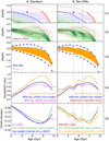 |
Fig. 5 Age–metallicity relations and gradient evolutions in our standard model (left column, compared to Lu et al. 2024a) and in the two-SFB model (right column, compared to Ratcliffe et al. 2023). Row 1: gaseous metallicity every two zones of the model. Row 2: density isocontours for the solar vicinity in the model (shaded, as in Fig. 2) and in Anders et al. (2023) (brown); the introduction of a SFB at 4.5 Gyr and 7 Gyr produces two local overdensities, as in the data. Row 3: age–metallicity relation in the solar vicinity with metallicity ranges indicated by mean±1 σ values (orange shaded area) and 95%-tiles (between the blue dotted curves featuring larger points every Gyr). Row 4: metallicity ranges Δ[Fe/H] (blue and orange curves derived from the data of same colour in the previous panels) and observationally inferred by Lu et al. (2024a, dashed magenta, left panel) and Ratcliffe et al. (2023, dashed red, right panel). Row 5: evolution of the abundance gradient, in observations from Lu et al. (2024a, dashed magenta, left panel) and Ratcliffe et al. (2023, dashed red, right panel), as well as in our model obtained either with our method of mass-weighted gradient (solid green curves in both panels, see text) or with the method of Lu et al. (2024a, solid blue, left panel) and Ratcliffe et al. (2023, solid orange, right panel). |
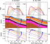 |
Fig. 6 Top: distribution of birth radii Rb of stars currently found in the solar vicinity (grey shaded area in all panels, extending from 7–9 kpc) for stars of different ages (in 1-Gyr wide bins, colour-coded by age), as predicted by our standard (left) and 2-SFB (right) models. Middle: radial metallicity profile of each mono-age population. The blue dots indicate boundaries including 95%-tiles of model local stars in the Rb distributions of the top panel. Bottom: the dashed lines represent the mass weighted (according to the distributions of the top panel) abundance gradient of each mono-age population. |
6.2 Results
The results of Fig. 6 can help one to understand the evolution of the abundance gradient at the birth radius inferred from local observations in our model. This evolution appears in the bottom panels of Fig. 5, where they are compared with the results of Lu et al. (2024a, displayed with magenta in A5) and Ratcliffe et al. (2023, orange in B5). The results are derived from two different methods: the one discussed in the previous paragraph (green in both bottom panels), and by adopting the same method as Lu et al. (2024a, blue in A5) and Ratcliffe et al. (2023, orange in B5), respectively.
The evolution of the gradient obtained in Lu et al. (2024a) is well reproduced in our standard model (A) both with our mass-weighted gradient and with the method of Lu et al. (2024a), as can be seen by comparing the solid green and blue curves with the purple dashed curve of the data in panel A5 of Fig. 5. The three left panels of Fig. 6 can help one to understand the gradient’s evolution. During the earliest period, the local stars observed today originate essentially from the innermost regions (RG<3 kpc, see panel A1 left in Fig. 6) where the metallicity profile was flat (A2 panel in same figure), providing a small slope (in absolute value) for the corresponding abundance gradient (panel A3 in the same figure). Progressively, the birthplace distribution of the presently local stars shifted to intermediate regions (3–5 kpc, panel A1 left) characterised by a steep abundance profile, thus increasing the absolute value of the negative abundance gradient. The increase stopped around the age of 9 Gyr, when the birthplace distributions started to be dominated by the regions around 5–8 kpc, where the abundance profile becomes progressively flatter and therefore the abundance gradient starts decreasing in absolute value. Thus, the maximum in absolute value observed around 9 Gyr corresponds to the end of a period of intense activity that had originally produced a flat profile in the inner disc and it left the outer disc with a very steep profile that progressively dominated the local stellar sample. This evolution of the abundance profile was also discussed in Prantzos et al. (2023), who found that the non-monotonic evolution of the abundance gradient at the birth radius naturally results through secular evolution, as do several other properties of the local disc. In contrast, Lu et al. (2024a) attribute it to the impact of a major merger (GES) on the metallicity profile of the Galaxy 8–10 Gyr ago.
In the case of model (B), a similar non-monotonic trend as in the baseline model is obtained, but this time two wiggles are superimposed, resulting from the action of the two SFBs. The effect of the SFBs is to rapidly increase the local metallicity, more in the outer regions than in the inner ones because the metallicity is smaller in the former and thus easier to increase. As a result, the metallicity difference between the inner and outer zones decreases during the SFBs. In fact, it is the Fe ejected by CCSN that is responsible for this outcome, as the Fe of SNIa is released on much longer time scales. When we adopted the method of Ratcliffe et al. (2023), that is, using the ‘mirror image’ of the metallicity range and adjusting the present-day and minimum values, our result is in fair agreement with the results of that work (solid orange versus dashed red curves, respectively, in panel B5 of Fig. 5).
On the other hand, our own method (using the mass-weighted gradient at the birthplace for all stars within a 1 Gyr-wide age bin) identifies the impact of the older SFB at the age of 7 Gyr with a slight time delay by about 0.3 Gyr, probably because it partially integrates the impact of the SNIa originating from that SFB. However, our method fails to clearly identify the impact of the younger SFB of age 4.5 Gyr. Only a change in the slope of the evolution of the gradient, again with a slight time delay, indicates the existence of some star formation episode at that time. The difference with respect to the case of the earlier SFB is due to the fact that at early times the mass-weighted gradient is determined by the stars of restricted regions in the inner disc, while at later timer it is smoothed over a large region of birth radii.
6.3 Discussion
After comparing the results obtained with the two different methods of analysis, we conclude that the idea of Lu et al. (2024a) may be applicable if the metallicity profile has a unique slope at any moment over the whole range of birth radii, but it leads to ambiguous results if the profile is a multi-slope one, as naturally obtained in the case of localized star formation episodes.
We note that in a recent work, Ratcliffe et al. (2024) have analysed MW/Andromeda analogues from the TNG50 simulation to study the possibility of recovering the behaviour of the metallicity profile at Rbirth as function of radius in a variety of galaxies. They find that the true central metallicity is unrepresentative of the genuine disc [Fe/H] profile and suggest to use a projected central metallicity instead. They claim that their method allows them ‘to expect to be able to recover Rbirth to within 1 kpc for the Milky Way disc’. Similarly, Lu et al. (2024b) have investigated the possibility of inferring birth radii for external galaxies such as the LMC using the NIHAO cosmological zoom-in simulations. They find that it is theoretically possible to do so, with a ~25% median uncertainty for individual stars, provided several conditions are fulfilled. However, the possibility of a gradient with a non-unique slope over the whole radial range is not considered in those studies.
7 SFB driven by gas dilution of the outer disc
In the previous sections, we considered SFBs induced by enhancement of the star formation efficiency due, for instance to perturbations from the passage of a nearby satellite galaxy. However, episodes of star formation may also be induced by events of strong gas accretion. Such events have a double effect. They first dilute the local gas metallicity and subsequently they increase it strongly, through the resulting strong star formation due to the larger gas reservoir. The latter effect will be particularly important if at the same time an enhanced star formation efficiency is assumed.
Such effects have been explored in some detail in Johnson & Weinberg (2020) with one-zone GCE models, without any connection to specific observational data. In a subsequent paper, Johnson et al. (2021) used a multi-ring model with parametrised stellar radial migration and applied it to the study of the MW. Within the framework of that model, they explored the consequences of a late and broad SFB, such as the one of Mor et al. (2019) on the present-day abundance gradients of Fe and O, but they provided no information regarding the impact of those SFBs on the evolution of the gradients.
The cosmological simulations of MW-mass galaxies by Buck et al. (2023) suggest that metal-poor cold gas from an early massive merger could dilute the metallicity in the outer disc regions and steepen an otherwise flat metallicity gas profile. This supports the Lu et al. (2024a) interpretation of their observed gradient inversion as being due to a major merger 8–9 Gyr ago, perhaps related to the thick-thin disc transition epoch. In an analogous way, Ratcliffe et al. (2023) attributed the two more recent fluctuations in the evolution of the abundance gradient to dilution episodes from gas accretion in the disc outskirts caused by passages of the Sgr galaxy which left behind substantial amounts of low metallicity gas.
In this section, we explore the consequences of those ideas by simulating two recent episodes of pristine (zero metallicity) infalling gas. We assumed episodes of Gaussian form, with maxima at ages of 6.3 Gyr and 3.7 Gyr ago, respectively, and standard deviations of 0.5 Gyr each. The infall episodes were assumed to occur in the outer disc, and their intensity decreases in the inner radii (it becomes null at 6 kpc). The time-integrated mass of accreted gas in each ring was normalised in order to be the same as in the standard case and to ensure the same total mass for the Galactic disc.
The comparison of the standard model and the one with two episodes of gas accretion are displayed in columns A and B, respectively, of Fig. 7. In the first row (panel B1) appear the two infall episodes, which are accompanied with a small time delay by enhanced star formation (panel B2). The late increase of gas mass in the outer disc reduces the difference of SFR between the inner and outer zones, when compared to the standard case (panel A2). In the subsequent rows of Fig. 7, we show the same results as Fig. 5. In panel B3, [Fe/H] in the gas of the outer regions is diluted by the additional primordial gas while the inner regions, unaffected by dilution, keep their steadily increasing trend of metallicity. Consequently, the metallicity range of stars found locally today increases during the dilution process (panels B5 and B6) and contracts right after that episode, because of the rapid Fe production through the enhanced star formation. This translates into a steepening of the Fe gradient followed by a flattening, and the same thing happens after the second dilution episode (panel B7).
The comparison to the data of Ratcliffe et al. (2023) in panel B7 is quite satisfactory, whether the gradient is evaluated through the mirror image of the range of [Fe/H] (orange curve) or with the weighted mean method (green curve) although the two methods do not provide exactly the same results. We emphasise that the oldest wiggle in panel B7 (at an age of 8–9 Gyr) is not due to any episode of SFR or gas accretion but simply to the migration of old stars from the inner regions, as it appears in panel A7 and is discussed in the previous section.
A careful comparison between Figs. 5 and 7 reveals an interesting feature. In the former case, the time of the star formation episode coincides with the maxima of the observationally inferred wiggles (see the vertical dashed curves throughout the figures). This is due to the fact that the SFBs in the outer disc enhance the metallicity in that region, pushing it closer to the metallicity of the inner one. As a result, the range of metallicities Δ[α/Fe] of mono-age populations found in the solar neighbourhood today is reduced and in the corresponding mirror image the metallicity gradient is increased, that is a maximum is obtained at the time of the star formation episode (panels B4 and B5 in Fig. 5. On the other hand, the infall episodes in the outer disc dilute the local metallicity and increase its difference with the metallicty in the inner regions. As a result, the range of metallicities Δ[α/Fe] of mono-age populations found in the solar neighbourhood today increases, and in its mirror image, a minimum is obtained (panels B5, B6 and B7 in Fig. 7). We believe that this property may help in the future, through improved age derminations, to better probe the nature of the interaction that produced the wiggles: enhanced SF efficiency in the first case versus infall episode in the second.
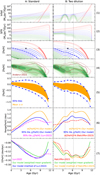 |
Fig. 7 Comparative evolution of several quantities for the baseline model (column A on the left) and the case of two recent infall episodes in the outer disc (column B on the right). Top: infall rate in various radial zones, with the curves colour-coded as in previous figures (red: inner zones, blue: intermediate, green: outer; thick dashed: 8 kpc). Second from top: corresponding local SFRs. The subsequent five rows of panels are the same as in Fig. 5. |
8 Discussion
As mentioned in Sect. 2.2, Ruiz-Lara et al. (2020) found star formation episodes ~5.7,1.9 and 1 Gyr ago and related them to pericentric passages of Sgr galaxy, which is commonly thought to be a highly possible perturber of the MW in the past (Peñarrubia et al. 2010; Gómez et al. 2013). This view is in agreement with the simulations of the Constrained Local UniversE simulations (CLUES) project of Di Cintio et al. (2021), where the host galaxies of infalling satellites show an enhancement of their star formation at pericentre passage. However, the authors emphasise that the this star formation enhancement depends on several factors, including the amount of gas of the perturber at pericentre and its distance to the host. Indeed, at very close passages, the gas of the perturber may be removed by ram pressure. In their high-resolution environmental simulations of the Local Group, which concern early mergers, Khoperskov et al. (2023) find a correlation between mergers and close pericentric passages of massive satellites and the bursts of the star formation in the in situ component of MW-type galaxies.
In addition, Annem & Khoperskov (2024) have made hydro-dynamical simulations of interactions of the MW-type galaxies with massive satellites, including gas-poor and gas-rich ones on quasi-polar orbits. They find a substantial increase in the SFR during close passages of gas-poor satellites. Such passages cause the formation of low-metallicity stars in the host, since the gas infall from the satellite results in the dilution of the local mean stellar metallicity of the host. They suggest that an SFB at ~6 Gyr, similar to the one found in Ruiz-Lara et al. (2020) could be attained through close passages (less than 20 kpc) of Sgr progenitor with subsequent non-negligible mass loss.
9 Summary
In this work with a semi-analytical model including radial migration, we have explored the consequences of recent star formation episodes – suggested by both observations and hydrodynamical simulations – on some chemical observables of the MW disc. We considered both local and global star formation episodes and in all cases we used the local SF history (in the solar neighbourood, inferred from those recent observations) as a key constraint. We focused, in particular, on the resulting evolution of metallicity and [α/Fe] ratios as well as of the metallicity gradient of stars at birth place.
We find that SF episodes induced by a temporary increase of the SF efficiency result in overdensities in the phase-space of various quantities, e.g. age versus metallicity, or [α/Fe] versus metallicity. These episodes also produce a rapid increase of both metallicity and [α/Fe] ratios. The increase is more pronounced in the case of local SF episodes than in global ones, under the constraint that both cases reproduce the observationally inferred local SF histories. The increase is also more pronounced for shorter SF episodes, such as those reported by Ruiz-Lara et al. (2020), than for long lasting ones, such as the one inferred in Mor et al. (2019). In all cases, the local metallicity distribution is broadened with respect to the ‘standard’ model with no SFBs, while the average age-metallicity relation of the local stellar population is distorted to a significant degree. Moreover, we found that the birthplace of the Sun has to move a little inwards (about 0.5–1.5 kpc) compared to the case of our ‘standard’ model (without SF episodes) presented in Prantzos et al. (2023).
We find that such SF episodes may increase the number of ‘young [α/Fe] -rich stars’ in the Galaxy, thus alleviating – but definitely not solving – the problem of their existence, first noticed by Chiappini et al. (2015) and Martig et al. (2015). Mergers between old [α/Fe] -rich stars of the thick disc, causing them to become more massive and therefore to appear younger, is the current popular explanation of that problem, e.g. Zhang et al. (2021); Miglio et al. (2021). We note, however, that a fraction of extreme [α/Fe] -rich dwarf stars in the GALAH survey has been shown to possess kinematics of thin disc stars and high Li content (Borisov et al. 2022), putting into question the merger interpretation.
In Prantzos et al. (2023), we found a non-monotonic behaviour of the local metallicity gradient of stars at their birth radius versus age in our ‘standard’ model. The locally observed abundance profile at the birth radius appears steeper at higher ages until a look-back time of 8–9 Gyr, where the trend is inversed. Such a relation was found empirically in Lu et al. (2024a), who attributed it to an old (8–9 Gyr ago) perturbation of the disc by a major merger, probably the GES. In this study we showed in detail (Sects. 6.1 and 6.2) how this gradient inversion is naturally obtained from the combined effects of the inside-out formation of the disc and radial migration. We also noticed that the method of Lu et al. (2024a) applies when the gaseous abundance profile is described by a unique slope over the whole radial range during the disc evolution, while in our model the profile is a muti-slope one.
We explored the impact of recent SF episodes on the evolution of the gradient at birthplace and we found that such SF episodes can explain the ‘wiggly’ behaviour of the gradient versus age found by Ratcliffe et al. (2023), provided that the times of the SF episodes are adjusted to the times of the wiggle maxima in that work (see Sect. 6.1 and Fig. 5). We also showed how a similar trend can obtained through intense infall episodes (see Sect. 7). An important difference between the two cases is that in the former it is the maxima of the wiggle that correspond to the time of the SF episodes, while in the latter it is the minima that correspond to the time of the infall episodes.
Finally we note that observations of gaseous abundance profiles in resolved galactic discs at high redshifts suggest that most of them undergo very little variation of the gradient with look-back time (Curti et al. 2020). This is in contrast with the significant evolution found in Lu et al. (2024a) and Ratcliffe et al. (2023) for the MW disc or in our models and in most inside-out schemes for disc formation. Various effects (turbulence, mergers, interactions) may mix the disc gas, leading to rather flat abundance profiles throughout the disc evolution, while in the absence of such effects discs may indeed develop a steep initial abundance profile that flattens with time, see e.g. Hemler et al. (2021) and references therein. It may well be that our Milky Way belongs to the latter case.
Acknowledgements
This study was conducted by Tianxiang Chen as a part of his PhD Thesis. Unfortunately, he passed away during the writing of the paper. It is dedicated to his memory.
References
- Abdurro’uf, Accetta, K., Aerts, C., et al. 2022, ApJS, 259, 35 [NASA ADS] [CrossRef] [Google Scholar]
- Anders, F., Chiappini, C., Rodrigues, T. S., et al. 2017, A&A, 597, A30 [NASA ADS] [CrossRef] [EDP Sciences] [Google Scholar]
- Anders, F., Gispert, P., Ratcliffe, B., et al. 2023, A&A, 678, A158 [NASA ADS] [CrossRef] [EDP Sciences] [Google Scholar]
- Annem, B., & Khoperskov, S. 2024, MNRAS, 527, 2426 [Google Scholar]
- Aumer, M., Binney, J., & Schönrich, R. 2016, MNRAS, 462, 1697 [NASA ADS] [CrossRef] [Google Scholar]
- Bailer-Jones, C. A. L., Rybizki, J., Fouesneau, M., Demleitner, M., & Andrae, R. 2021, AJ, 161, 147 [Google Scholar]
- Belokurov, V., Erkal, D., Evans, N. W., Koposov, S. E., & Deason, A. J. 2018, MNRAS, 478, 611 [Google Scholar]
- Beraldo e Silva, L., Debattista, V. P., Nidever, D., Amarante, J. A. S., & Garver, B. 2021, MNRAS, 502, 260 [NASA ADS] [CrossRef] [Google Scholar]
- Bigiel, F., Leroy, A., Walter, F., et al. 2008, AJ, 136, 2846 [NASA ADS] [CrossRef] [Google Scholar]
- Blitz, L. & Rosolowsky, E. 2006, ApJ, 650, 933 [NASA ADS] [CrossRef] [Google Scholar]
- Boissier, S., & Prantzos, N. 1999, MNRAS, 307, 857 [NASA ADS] [CrossRef] [Google Scholar]
- Borisov, S., Prantzos, N., & Charbonnel, C. 2022, A&A, 668, A181 [NASA ADS] [CrossRef] [EDP Sciences] [Google Scholar]
- Buck, T. 2020, MNRAS, 491, 5435 [NASA ADS] [CrossRef] [Google Scholar]
- Buck, T., Obreja, A., Ratcliffe, B., et al. 2023, MNRAS, 523, 1565 [CrossRef] [Google Scholar]
- Buder, S., Sharma, S., Kos, J., et al. 2021, MNRAS, 506, 150 [NASA ADS] [CrossRef] [Google Scholar]
- Cartledge, S. I. B., Lauroesch, J. T., Meyer, D. M., & Sofia, U. J. 2006, ApJ, 641, 327 [NASA ADS] [CrossRef] [Google Scholar]
- Cerqui, V., Haywood, M., Di Matteo, P., Katz, D., & Royer, F. 2023, A&A, 676, A108 [NASA ADS] [CrossRef] [EDP Sciences] [Google Scholar]
- Chiappini, C., Matteucci, F., & Gratton, R. 1997, ApJ, 477, 765 [Google Scholar]
- Chiappini, C., Anders, F., & Minchev, I. 2014, in EAS Publications Series, 67–68, 169 [Google Scholar]
- Chiappini, C., Anders, F., Rodrigues, T. S., et al. 2015, A&A, 576, L12 [NASA ADS] [CrossRef] [EDP Sciences] [Google Scholar]
- Cristallo, S., Straniero, O., Piersanti, L., & Gobrecht, D. 2015, ApJS, 219, 40 [Google Scholar]
- Curti, M., Maiolino, R., Cirasuolo, M., et al. 2020, MNRAS, 492, 821 [CrossRef] [Google Scholar]
- Diaz, A. I., & Tosi, M. 1984, MNRAS, 208, 365 [NASA ADS] [CrossRef] [Google Scholar]
- Di Cintio, A., Mostoghiu, R., Knebe, A., & Navarro, J. F. 2021, MNRAS, 506, 531 [NASA ADS] [CrossRef] [Google Scholar]
- Feltzing, S., Bowers, J. B., & Agertz, O. 2020, MNRAS, 493, 1419 [Google Scholar]
- Ferrini, F., Molla, M., Pardi, M. C., & Diaz, A. I. 1994, ApJ, 427, 745 [CrossRef] [Google Scholar]
- Feuillet, D. K., Frankel, N., Lind, K., et al. 2019, MNRAS, 489, 1742 [Google Scholar]
- Frankel, N., Rix, H.-W., Ting, Y.-S., Ness, M., & Hogg, D. W. 2018, ApJ, 865, 96 [NASA ADS] [CrossRef] [Google Scholar]
- Fu, J., Hou, J. L., Yin, J., & Chang, R. X. 2009, ApJ, 696, 668 [NASA ADS] [CrossRef] [Google Scholar]
- Gaia Collaboration (Vallenari, A., et al.) 2023, A&A, 674, A1 [NASA ADS] [CrossRef] [EDP Sciences] [Google Scholar]
- Gibson, B. K., Pilkington, K., Brook, C. B., Stinson, G. S., & Bailin, J. 2013, A&A, 554, A47 [CrossRef] [EDP Sciences] [Google Scholar]
- Gilmore, G., & Wyse, R. F. G. 1991, ApJ, 367, L55 [NASA ADS] [CrossRef] [Google Scholar]
- Gómez, F. A., Minchev, I., O’Shea, B. W., et al. 2013, MNRAS, 429, 159 [Google Scholar]
- Grisoni, V., Spitoni, E., & Matteucci, F. 2018, MNRAS, 481, 2570 [NASA ADS] [Google Scholar]
- Grisoni, V., Chiappini, C., Miglio, A., et al. 2024, A&A, 683, A111 [NASA ADS] [CrossRef] [EDP Sciences] [Google Scholar]
- Hammer, F., Puech, M., Chemin, L., Flores, H., & Lehnert, M. D. 2007, ApJ, 662, 322 [NASA ADS] [CrossRef] [Google Scholar]
- Hayden, M. R., Bovy, J., Holtzman, J. A., et al. 2015, ApJ, 808, 132 [Google Scholar]
- Helmi, A. 2020, ARA&A, 58, 205 [Google Scholar]
- Helmi, A., Babusiaux, C., Koppelman, H. H., et al. 2018, Nature, 563, 85 [Google Scholar]
- Hemler, Z. S., Torrey, P., Qi, J., et al. 2021, MNRAS, 506, 3024 [NASA ADS] [CrossRef] [Google Scholar]
- Hidalgo, S. L., Pietrinferni, A., Cassisi, S., et al. 2018, ApJ, 856, 125 [Google Scholar]
- Hou, J. L., Prantzos, N., & Boissier, S. 2000, A&A, 362, 921 [NASA ADS] [Google Scholar]
- Isern, J. 2019, ApJ, 878, L11 [NASA ADS] [CrossRef] [Google Scholar]
- Iwamoto, K., Brachwitz, F., Nomoto, K., et al. 1999, ApJS, 125, 439 [NASA ADS] [CrossRef] [Google Scholar]
- Jofré, P., Jorissen, A., Van Eck, S., et al. 2016, A&A, 595, A60 [Google Scholar]
- Johnson, J. W., & Weinberg, D. H. 2020, MNRAS, 498, 1364 [CrossRef] [Google Scholar]
- Johnson, J. W., Weinberg, D. H., Vincenzo, F., et al. 2021, MNRAS, 508, 4484 [NASA ADS] [CrossRef] [Google Scholar]
- Kennicutt, J., Robert C. 1998, ApJ, 498, 541 [NASA ADS] [CrossRef] [Google Scholar]
- Khoperskov, S., Minchev, I., Libeskind, N., et al. 2023, A&A, 677, A89 [NASA ADS] [CrossRef] [EDP Sciences] [Google Scholar]
- Kobayashi, C., & Nakasato, N. 2011, ApJ, 729, 16 [NASA ADS] [CrossRef] [Google Scholar]
- Kroupa, P. 2002, Science, 295, 82 [Google Scholar]
- Krumholz, M. R. 2014, Phys. Rep., 539, 49 [Google Scholar]
- Kubryk, M., Prantzos, N., & Athanassoula, E. 2015a, A&A, 580, A126 [NASA ADS] [CrossRef] [EDP Sciences] [Google Scholar]
- Kubryk, M., Prantzos, N., & Athanassoula, E. 2015b, A&A, 580, A127 [NASA ADS] [CrossRef] [EDP Sciences] [Google Scholar]
- Limongi, M., & Chieffi, A. 2018, ApJS, 237, 13 [NASA ADS] [CrossRef] [Google Scholar]
- Lu, Y., Buck, T., Minchev, I., & Ness, M. K. 2022, MNRAS, 515, L34 [NASA ADS] [CrossRef] [Google Scholar]
- Lu, Y., Minchev, I., Buck, T., et al. 2024a, MNRAS, 535, 392 [NASA ADS] [CrossRef] [Google Scholar]
- Lu, Y., Buck, T., Nidever, D., et al. 2024b, MNRAS, 532, 411 [NASA ADS] [CrossRef] [Google Scholar]
- Maciel, W. J., Lago, L. G., & Costa, R. D. D. 2006, A&A, 453, 587 [NASA ADS] [CrossRef] [EDP Sciences] [Google Scholar]
- Maciel, W. J., Quireza, C., & Costa, R. D. D. 2007, A&A, 463, L13 [NASA ADS] [CrossRef] [EDP Sciences] [Google Scholar]
- Magrini, L., Randich, S., Kordopatis, G., et al. 2017, A&A, 603, A2 [NASA ADS] [CrossRef] [EDP Sciences] [Google Scholar]
- Magrini, L., Viscasillas Vázquez, C., Spina, L., et al. 2023, A&A, 669, A119 [NASA ADS] [CrossRef] [EDP Sciences] [Google Scholar]
- Martig, M., Rix, H.-W., Silva Aguirre, V., et al. 2015, MNRAS, 451, 2230 [NASA ADS] [CrossRef] [Google Scholar]
- Miglio, A., Chiappini, C., Mackereth, J. T., et al. 2021, A&A, 645, A85 [NASA ADS] [CrossRef] [EDP Sciences] [Google Scholar]
- Minchev, I., Chiappini, C., & Martig, M. 2013, A&A, 558, A9 [CrossRef] [EDP Sciences] [Google Scholar]
- Minchev, I., Anders, F., Recio-Blanco, A., et al. 2018, MNRAS, 481, 1645 [NASA ADS] [CrossRef] [Google Scholar]
- Mints, A., & Hekker, S. 2017, A&A, 604, A108 [NASA ADS] [CrossRef] [EDP Sciences] [Google Scholar]
- Mollá, M., Díaz, Á. I., Ascasibar, Y., & Gibson, B. K. 2017, MNRAS, 468, 305 [CrossRef] [Google Scholar]
- Mollá, M., Díaz, Á. I., Cavichia, O., et al. 2019, MNRAS, 482, 3071 [NASA ADS] [Google Scholar]
- Montalbán, J., Mackereth, J. T., Miglio, A., et al. 2021, Nat. Astron., 5, 640 [Google Scholar]
- Mor, R., Robin, A. C., Figueras, F., Roca-Fàbrega, S., & Luri, X. 2019, A&A, 624, L1 [NASA ADS] [CrossRef] [EDP Sciences] [Google Scholar]
- Mott, A., Spitoni, E., & Matteucci, F. 2013, MNRAS, 435, 2918 [Google Scholar]
- Nieva, M. F., & Przybilla, N. 2012, A&A, 539, A143 [NASA ADS] [CrossRef] [EDP Sciences] [Google Scholar]
- Nissen, P. E., Christensen-Dalsgaard, J., Mosumgaard, J. R., et al. 2020, A&A, 640, A81 [NASA ADS] [CrossRef] [EDP Sciences] [Google Scholar]
- Peñarrubia, J., Belokurov, V., Evans, N. W., et al. 2010, MNRAS, 408, L26 [NASA ADS] [Google Scholar]
- Philcox, O., Rybizki, J., & Gutcke, T. A. 2018, ApJ, 861, 40 [Google Scholar]
- Pilkington, K., Few, C. G., Gibson, B. K., et al. 2012, A&A, 540, A56 [NASA ADS] [CrossRef] [EDP Sciences] [Google Scholar]
- Prantzos, N., Abia, C., Limongi, M., Chieffi, A., & Cristallo, S. 2018, MNRAS, 476, 3432 [Google Scholar]
- Prantzos, N., Abia, C., Cristallo, S., Limongi, M., & Chieffi, A. 2020, MNRAS, 491, 1832 [Google Scholar]
- Prantzos, N., Abia, C., Chen, T., et al. 2023, MNRAS, 523, 2126 [NASA ADS] [CrossRef] [Google Scholar]
- Queiroz, A. B. A., Anders, F., Chiappini, C., et al. 2023, A&A, 673, A155 [NASA ADS] [CrossRef] [EDP Sciences] [Google Scholar]
- Ratcliffe, B., Minchev, I., Anders, F., et al. 2023, MNRAS, 525, 2208 [NASA ADS] [CrossRef] [Google Scholar]
- Ratcliffe, B., Khoperskov, S., Minchev, I., et al. 2024, A&A, 690, A352 [NASA ADS] [CrossRef] [EDP Sciences] [Google Scholar]
- Ritchey, A. M., Jenkins, E. B., Shull, J. M., et al. 2023, ApJ, 952, 57 [NASA ADS] [CrossRef] [Google Scholar]
- Ruiz-Lara, T., Gallart, C., Bernard, E. J., & Cassisi, S. 2020, Nat. Astron., 4, 965 [NASA ADS] [CrossRef] [Google Scholar]
- Sahlholdt, C. L., Feltzing, S., & Feuillet, D. K. 2022, MNRAS, 510, 4669 [NASA ADS] [CrossRef] [Google Scholar]
- Salaris, M., Chieffi, A., & Straniero, O. 1993, ApJ, 414, 580 [NASA ADS] [CrossRef] [Google Scholar]
- Sanders, J. L., & Binney, J. 2015, MNRAS, 449, 3479 [NASA ADS] [CrossRef] [Google Scholar]
- Schmidt, M. 1959, ApJ, 129, 243 [NASA ADS] [CrossRef] [Google Scholar]
- Schmidt, M. 1963, ApJ, 137, 758 [Google Scholar]
- Schönrich, R., & Binney, J. 2009, MNRAS, 396, 203 [Google Scholar]
- Sellwood, J. A., & Binney, J. J. 2002, MNRAS, 336, 785 [Google Scholar]
- Siegel, M. H., Dotter, A., Majewski, S. R., et al. 2007, ApJ, 667, L57 [NASA ADS] [CrossRef] [Google Scholar]
- Soderblom, D. R. 2010, ARA&A, 48, 581 [Google Scholar]
- Spitoni, E., Matteucci, F., Gratton, R., et al. 2024, A&A, 690, A208 [NASA ADS] [CrossRef] [EDP Sciences] [Google Scholar]
- Tissera, P. B., Machado, R. E. G., Vilchez, J. M., et al. 2017, A&A, 604, A118 [NASA ADS] [CrossRef] [EDP Sciences] [Google Scholar]
- Vincenzo, F., & Kobayashi, C. 2020, MNRAS, 496, 80 [NASA ADS] [CrossRef] [Google Scholar]
- Weinberg, D. H., Andrews, B. H., & Freudenburg, J. 2017, ApJ, 837, 183 [NASA ADS] [CrossRef] [Google Scholar]
- Zhang, M., Xiang, M., Zhang, H.-W., et al. 2021, ApJ, 922, 145 [NASA ADS] [CrossRef] [Google Scholar]
http://fruity.oa-abruzzo.inaf.it and http://orfeo.iaps.inaf.it/index.html for LIMS and massive stars, respectively.
In all the models, the star formation efficiency is adjusted so as to lead to an approximately solar metallicity in the local ISM today.
All Figures
|
Fig. 1 Recently reported episodes of star formation in the late history of the local region of our Galaxy. From top to bottom: (a) SFR obtained from main-sequence stars (Mor et al. 2019), with error bars in age and SFR intensity. (b) The cyan curve represents the SFH in a bubble of radius ∼2 kpc around the Sun (Ruiz-Lara et al. 2020). The three subsequent panels display results for age distribution of stars obtained from Sahlholdt et al. (2022) for (c) the inner, (d) the local and (e) the outer Galactic disc; in those three panels dashed curves correspond to the situation close to the plane and dotted ones away from the plane, with solid curve representing the total (in percentage). The age range of all data is normalised to the time duration of our model (Tmax = 12 Gyr). In (a) and (b), observations are normalised to the present-day local star surface density (38 M⊙ /pc2) with the adopted IMF of Kroupa (2002). The two vertical lines are to guide the eye and correspond to the centroids of the SFB of Mor et al. (2019), of the strongest SFB of Ruiz-Lara et al. (2020) and of the first SFB of Sahlholdt et al. (2022). |
| In the text | |
|
Fig. 2 Comparison of various quantities as function of age among models with five different SFHs (standard, single local SFB, single global SFB, three local SFBs, and three global SFBs). Row 1: true SFR in different radial zones, divided into inner disc (R < 5 kpc, red), intermediate disc (5 < R < 11 kpc, blue) and outer disc (R > 11 kpc, green). The evolution at R⊙ = 8 kpc is depicted by dashed blue curve. Row 2: SFH as observed today in the solar cylinder (7 < R < 9 kpc) after counting stellar radial migration. The vertical dotted line at 9 Gyr separates the disc (age >9 Gyr, red) from the disc (age <9 Gyr, blue). Row 3: evolution of [Fe/H] in the gas in different radial zones. Thick portions of curves indicate the periods of SFR higher than the time-averaged one. Row 4: [Fe/H] of stars existing in solar cylinder at the end of the simulation. The colour-coded filled contours represent the number density of stars. As shown on the left colour bar, the contour levels correspond to the fractions of 0.001, 0.1, 0.3, 0.5, 0.7, 0.9 of the total numbers of stars. The red and blue curves indicate the average [Fe/H] of the thin and thick discs. Row 5: evolution of [Si/Fe] in the gas in different radial zones. Row 6: [Si/Fe] in stars found in the solar cylinder at the end of the simulation. The fraction of young α-enhanced stars selected using the criterion from Chiappini et al. (2014) (magenta) and Zhang et al. (2021) (brown) are shown on the top left, along with the corresponding fractions of stars in those regions as obtained by our models (see text). Orange dots denote young, high [α/Fe] stars from Miglio et al. (2021). |
| In the text | |
|
Fig. 3 Model results (colour coded as in Fig. 2) and comparison to observations for various quantities as function of [Fe/H], Row 1: metallicity distributions for thin (blue) and thick (red) discs in the solar cylinder. The thin ones are compared to the red giants near the plane (|ɀ| < 0.3 kpc) from the APOGEE DR17 (dotted grey). Row 2: age-metallicity relation for all radial zones. Row 3: predicted age versus [Fe/H] distribution present in the solar cylinder. The average ages of thin and thick discs (red and blue curves) are compared to data from Feuillet et al. (2019) shown by orange curves with vertical error bars. Row 4: gas evolution of the various radial zones of the model in the [Si/Fe]-[Fe/H] plane. Row 5: predicted [Si/Fe] versus [Fe/Hl distribution present in solar cylinder. |
| In the text | |
|
Fig. 4 Results of the propagated SFB model. Left: same as the second and fourth row of Fig. 2, for the evolution of SFR and [M/H], Right: age distributions are displayed in the top panel for different radial ranges of 6–7, 7–9 and 9–10 kpc, corresponding to the equivalent observational sub-samples in inner, local, and outer bins shown in Fig. 6 of Sahlholdt et al. (2022); observations (red curves) are compared to model results (blue curves). In the lower panels, age–metallicity relations of the model (green isodensity contours) are compared to half-maximum density contours from observations of Sahlholdt et al. (2022) (dotted and dashed red curves indicate the high-ɀmax and low-ɀmax part of observations in each radial range). |
| In the text | |
|
Fig. 5 Age–metallicity relations and gradient evolutions in our standard model (left column, compared to Lu et al. 2024a) and in the two-SFB model (right column, compared to Ratcliffe et al. 2023). Row 1: gaseous metallicity every two zones of the model. Row 2: density isocontours for the solar vicinity in the model (shaded, as in Fig. 2) and in Anders et al. (2023) (brown); the introduction of a SFB at 4.5 Gyr and 7 Gyr produces two local overdensities, as in the data. Row 3: age–metallicity relation in the solar vicinity with metallicity ranges indicated by mean±1 σ values (orange shaded area) and 95%-tiles (between the blue dotted curves featuring larger points every Gyr). Row 4: metallicity ranges Δ[Fe/H] (blue and orange curves derived from the data of same colour in the previous panels) and observationally inferred by Lu et al. (2024a, dashed magenta, left panel) and Ratcliffe et al. (2023, dashed red, right panel). Row 5: evolution of the abundance gradient, in observations from Lu et al. (2024a, dashed magenta, left panel) and Ratcliffe et al. (2023, dashed red, right panel), as well as in our model obtained either with our method of mass-weighted gradient (solid green curves in both panels, see text) or with the method of Lu et al. (2024a, solid blue, left panel) and Ratcliffe et al. (2023, solid orange, right panel). |
| In the text | |
|
Fig. 6 Top: distribution of birth radii Rb of stars currently found in the solar vicinity (grey shaded area in all panels, extending from 7–9 kpc) for stars of different ages (in 1-Gyr wide bins, colour-coded by age), as predicted by our standard (left) and 2-SFB (right) models. Middle: radial metallicity profile of each mono-age population. The blue dots indicate boundaries including 95%-tiles of model local stars in the Rb distributions of the top panel. Bottom: the dashed lines represent the mass weighted (according to the distributions of the top panel) abundance gradient of each mono-age population. |
| In the text | |
|
Fig. 7 Comparative evolution of several quantities for the baseline model (column A on the left) and the case of two recent infall episodes in the outer disc (column B on the right). Top: infall rate in various radial zones, with the curves colour-coded as in previous figures (red: inner zones, blue: intermediate, green: outer; thick dashed: 8 kpc). Second from top: corresponding local SFRs. The subsequent five rows of panels are the same as in Fig. 5. |
| In the text | |
Current usage metrics show cumulative count of Article Views (full-text article views including HTML views, PDF and ePub downloads, according to the available data) and Abstracts Views on Vision4Press platform.
Data correspond to usage on the plateform after 2015. The current usage metrics is available 48-96 hours after online publication and is updated daily on week days.
Initial download of the metrics may take a while.