


| Issue |
A&A
Volume 712, August 2026
|
|
|---|---|---|
| Article Number | A20 | |
| Number of page(s) | 19 | |
| Section | Extragalactic astronomy | |
| DOI | https://doi.org/10.1051/0004-6361/202558018 | |
| Published online | 30 July 2026 | |
X-ray luminosity function of Compton-thick active galactic nuclei in the early Universe (z ≥ 3)
Robustness and biases of the CTK population
IAASARS, National Observatory of Athens, Ioannou Metaxa and Vasileos Pavlou, GR-15236 Athens, Greece
★ Corresponding author: This email address is being protected from spambots. You need JavaScript enabled to view it.
Received:
7
November
2025
Accepted:
8
June
2026
Abstract
The population of Compton-thick (CTK) active galactic nuclei (AGNs) represents a critical yet elusive phase in the growth of supermassive black holes (SMBHs). Constraining their abundance and evolution at high redshift is essential for understanding both SMBH growth and the origin of the cosmic X-ray background. We investigate the X-ray luminosity function (XLF) of CTK AGNs at z ≥ 3 using one of the largest available samples of X-ray-selected AGNs at high redshifts, containing 811 sources from XMM-Newton XXL-N and Chandra CCLS and CDF-S/N surveys. We first selected a subsample of ten high-probability CTK candidates, identified through Bayesian X-ray spectral fitting. Their multiwavelength properties are examined through spectral energy distribution modelling to assess the robustness of their CTK classification. For most sources, the inferred X-ray luminosities – and consequently their hydrogen column densities (NH) – appear overestimated when compared with their infrared (IR) luminosities. After updating the NH posteriors with IR-informed priors, only three sources remained consistent with the CTK regime. To compute the XLF for the entire CTK AGN population, we used 24 μm photometry to estimate IR luminosities and update the X-ray posteriors for all the remaining sources. Incorporating IR priors systematically reduces the inferred CTK number densities, yielding a more conservative and physically consistent estimate of the X-ray luminosity and absorption functions. We find that CTK AGNs constitute 17+12−11% of the total AGN population at 3 ≤ z ≤ 6, consistent with results at lower redshifts. Our analysis reveals no statistically significant evolution in the CTK fraction up to z ∼ 6, suggesting that the most heavily obscured accretion phase remains a persistent component of black hole growth throughout cosmic history. While the overall obscured AGN fraction (NH > 1023 cm−2) increases toward higher redshifts, the stable CTK fraction supports the interpretation that, at these epochs, the interstellar medium in typical host galaxies cannot produce CTK levels of obscuration.
Key words: methods: observational / methods: statistical / galaxies: active / infrared: galaxies / X-rays: galaxies
© The Authors 2026
 Open Access article, published by EDP Sciences, under the terms of the Creative Commons Attribution License (https://creativecommons.org/licenses/by/4.0), which permits unrestricted use, distribution, and reproduction in any medium, provided the original work is properly cited.
This article is published in open access under the Subscribe to Open model. This email address is being protected from spambots. You need JavaScript enabled to view it. to support open access publication.
1. Introduction
Active galactic nuclei (AGNs) are among the most luminous sources in the Universe. They are powered by accretion onto supermassive black holes (SMBHs) in their centres (Lynden-Bell 1969). These black holes typically have masses in the range 106 − 109 M⊙. Matter infalling towards the SMBH forms an accretion disc that radiates in the extreme ultraviolet (UV), while X-rays are produced by inverse Compton scattering of these photons in a hot corona of electrons above the disc (e.g. Haardt & Maraschi 1991). The primary X-ray emission is often absorbed by gas and dust (Alexander & Hickox 2012; Brandt & Alexander 2015; Netzer 2015), in what has historically been interpreted as a toroidal structure (Antonucci & Miller 1985), though infrared (IR) and millimetre imaging has revealed a more complex morphology (Hönig et al. 2012; García-Burillo et al. 2016).
Because X-rays penetrate high column densities, they offer a powerful means of tracing AGN activity across cosmic time. Observations with Chandra and XMM-Newton have mapped the accretion history of SMBHs up to z ∼ 3 (e.g. Ueda et al. 2014; Aird et al. 2015b; Buchner et al. 2015; Miyaji et al. 2015; Fotopoulou et al. 2016; Georgakakis et al. 2017). At higher redshifts (z = 3 − 6), the AGN luminosity function has been explored by Georgakakis et al. (2015), Vito et al. (2018), and Pouliasis et al. (2024), who showed that AGNs were more abundant at earlier epochs, with the number density peak depending on luminosity. These studies also established that obscuration increases with redshift: the fraction of obscured AGNs with log NH > 23 rises from ∼50% at z ≈ 1 (Signorini et al. 2023; Vijarnwannaluk et al. 2024) to ∼75% at z ≥ 3 (Vito et al. 2018; Pouliasis et al. 2024). Lower column densities of the order of log NH ∼ 22 cannot be easily constrained at high redshifts as the obscuration low-energy turnover is redshifted out of the XMM-Newton and Chandra bandpass. The increase of the column density with redshift likely reflects the higher gas and dust content of early galaxies, as supported by The Atacama Large Millimetre/submillimetre Array (ALMA) observations (Scoville et al. 2017; Gilli et al. 2022).
For column densities above log NH ≈ 24, gas becomes optically thick to Compton scattering, defining the Compton-thick (CTK) regime. CTK AGNs are key to understanding SMBH growth, AGN–galaxy co-evolution, and the origin of the cosmic X-ray background (Comastri et al. 1995; Gilli et al. 2007; Akylas et al. 2012; Ananna et al. 2019). Hard X-ray (14−195 keV) surveys with Swift/BAT (Burst Alert Telescope; Barthelmy et al. 2005) have provided robust constraints in the local Universe (z ≲ 0.1), yielding observed CTK fractions of ≲20% (Burlon et al. 2011; Akylas et al. 2016; Georgantopoulos & Akylas 2019; Torres-Albà et al. 2021) and intrinsic fractions of ∼20 − 30% after flux bias corrections (Ricci et al. 2015; Akylas et al. 2024; Annuar et al. 2025).
The broad energy range of the Nuclear Spectroscopic Telescope Array (NuSTAR) detectors (8−79 keV) makes it a powerful tool for the study of CTK-AGNs though its sensitivity limits its ability to study obscured AGNs in the high-redshift (z > 3) regime. Recent studies based on NuSTAR observations yield similar results for the fraction of CTK AGNs in the local Universe (Boorman et al. 2025; Georgantopoulos et al. 2025). Ananna et al. (2019) reported a fraction of CTK-AGNs in the local universe (z ≈ 0.1) that can reach up 50 ± 9% provided that extremely obscured sources with log NH > 25 are taken into account. This result is derived from a population synthesis model that fits the observed cosmic X-ray background in the 0.5−100 keV energy range.
Beyond the local Universe, CTK AGNs have been systematically identified up to about z = 3 using Chandra and XMM-Newton (e.g. Georgantopoulos et al. 2013; Brightman et al. 2014; Buchner et al. 2015; Lanzuisi et al. 2015, 2018; Georgakakis et al. 2017; Laloux et al. 2023), but their fraction and evolution remain uncertain. Buchner et al. (2015) reported a CTK fraction of 43 ± 10% with no clear redshift dependence, whereas Lanzuisi et al. (2018) found evidence of a strong evolution, reaching ∼45% at z > 2. More recently, Laloux et al. (2023) introduced a method combining X-ray spectra with IR priors, enabling the rejection of spurious CTK classifications. Their results are consistent with the local BAT estimates and with no significant evolution of the CTK fraction.
In this work, we revisit the CTK AGN luminosity function at z > 3 using the XMM-Newton XXL-N, Chandra COSMOS Legacy, and Chandra Deep Field (South and North) surveys. Building on Pouliasis et al. (2024), who derived the X-ray luminosity and absorption function (XLAF) for z = 3 − 6, we focus here on the CTK regime (NH ≥ 1024 cm−2). We re-evaluated CTK candidates through multiwavelength analysis and compared their intrinsic X-ray and IR luminosities to assess the reliability of their CTK classification. These effects were then taken into account to calculate the luminosity function for CTK AGNs in a more conservative and physically consistent way.
The paper is organised as follows: Sect. 2 describes the initial high-redshift sample and CTK candidate selection; Sect. 3 presents the analysis and results; Sect. 4 discusses our findings; and Sect. 5 summarises our conclusions. Throughout this paper, we adopt a Λ cold dark matter cosmology with H0 = 70 km s−1 Mpc−1, Ωm = 0.3, and ΩΛ = 0.7 (Komatsu et al. 2009).
2. Data and sample selection
In Pouliasis et al. (2024) we presented one of the largest samples of high-redshift (z ≥ 3), X-ray-selected (0.5−2 keV band) AGNs, comprising 811 sources. The sample was assembled using data from three major X-ray surveys: Chandra Deep Field South and North (CDF-S/N; Luo et al. 2017; Xue et al. 2016), Chandra COSMOS Legacy Survey (CCLS; Civano et al. 2016), and the northern field of the XMM-Newton XXL survey (XXL-N; Pierre et al. 2016). The combination of survey depths and sky areas provides broad coverage in X-ray luminosity, redshift, and absorption column density.
The high optical identification rates of these surveys allow the construction of a highly complete sample in terms of distance information, based on either spectroscopic redshifts, when available, or probabilistic photometric redshifts. For the Chandra surveys, Pouliasis et al. (2024) adopted photometric redshifts from the literature (Vito et al. 2018; Marchesi et al. 2016), while for XXL-N, new photometric redshifts were derived using deeper optical imaging from the Hyper Suprime-Cam (HSC) survey (Miyazaki et al. 2018). The final Pouliasis et al. (2024) sample includes all sources with spectroscopic redshifts z ≥ 3 (191 sources) and those with photometric redshifts having a probability greater than 20% of being at z ≥ 3 (620 sources). When weighting the photometric-redshift sources by their high-redshift probabilities, the effective total number of sources is 631.2.
X-ray spectra for all sources were extracted using the standard tools for the corresponding missions, CIAO (v4.13) for Chandra and SAS (v19) for XMM-Newton (see Sect. 3.1 of Pouliasis et al. 2024, for details) and modelled using the Bayesian X-ray analysis framework (BXA; Buchner et al. 2014; Buchner 2021) in combination with the UXClumpy torus model (Buchner et al. 2019) to estimate intrinsic X-ray properties (see Sect. 3.2 of Pouliasis et al. 2024, for details on the X-ray spectral modelling) such as absorption-corrected 2−10 keV luminosities (LX) and hydrogen column densities (NH)1. For each source, this procedure yields a posterior probability distribution in redshift, luminosity, and absorption, P(z, log LX, log NH|X).
Pouliasis et al. (2024) used these posteriors to derive a parametric model for the joint XLAF of AGNs (see Appendix A for a detailed description of the methodology employed) with 3 ≤ z ≤ 6 and 20 ≤ log NH ≤ 26, focusing primarily on the unabsorbed and Compton-thin (22 ≤ log NH ≤ 24) regime. In the present work, we extend this analysis to the CTK domain, aiming to assess the reliability of X-ray spectral constraints for potential CTK candidates. To this end, we selected a subsample of sources with a high probability of being CTK, based solely on their X-ray properties, as described in Sect. 2.1.
2.1. Sample of CTK AGNs
We identified compelling candidates for high-redshift CTK AGNs within the Pouliasis et al. (2024) sample. Using the posterior probability distributions derived from the X-ray spectral analysis, we computed the marginalised 1D probabilities for z and log NH and selected sources with a probability exceeding 80% of having z > 2.5 and log NH > 24. Twelve sources satisfied these criteria.
We then visually inspected the optical and IR images of these 12 sources to confirm the correct counterparts. Two XXL-N sources (hz428174 and hz414292) were found to have incorrect associations; we recalculated their photometric redshifts using the corrected photometry, after which only hz414292 remained in the sample. One CDF-S source (cdfs412) had an erroneous spectroscopic redshift; its photometric redshift falls below our selection threshold, and it was therefore excluded from the sample. One source in CDF-N (cdfn257) has a JWST spectrum with z = 2.95, consistent with our initial photometric redshift estimate. We re-ran the X-ray spectral analysis for all sources with updated redshifts. The final sample comprises ten sources, listed in Table 1. Figure 1 shows the 2−10 keV luminosity versus the hydrogen column density for the full Pouliasis et al. (2024) sample, highlighting the selected CTK candidates.
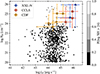 |
Fig. 1. Intrinsic X-ray luminosity in the 2−10 keV band versus hydrogen column density. Small circles show the full sample from Pouliasis et al. (2024), shaded by the probability of being CTK. Large circles mark our selection of CTK candidates, as described in Sect. 2.1, colour-coded according to their parent X-ray survey: CDF (yellow), CCLS (red), XXL-N (blue). For clarity, error bars (indicating 90% credible intervals) are shown only for the CTK candidates. |
High-redshift CTK candidates.
2.2. Multiwavelength counterparts
We compiled multiwavelength photometric data, spanning from the optical to mid-infrared (MIR) regime, for our sample of CTK AGNs using publicly available catalogues from the literature.
For sources in the XXL-N field, we adopted the photometric catalogue of Pouliasis et al. (2024), which incorporates deeper imaging from recent public data releases and updates the earlier compilation of Pouliasis et al. (2022). This catalogue provides optical photometry from HSC (g, r, i, z, Y bands; Miyazaki et al. 2018), complemented by u-band data from the Canada France Hawaii Telescope (CFHT; Sawicki et al. 2019), and near-infrared (NIR) measurements (J, H, Ks) from UKIDSS (DXS/UDS; Lawrence et al. 2007) and from several VISTA surveys: VHS (Vista Hemisphere Survey, McMahon et al. 2013), VIKING (VISTA Kilo-degree Infrared Galaxy, Edge et al. 2013) and VIDEO (VISTA Deep Extragalactic Observations, Jarvis et al. 2013). We further supplemented this dataset with MIR photometry from the Spitzer enhanced imaging products (SEIP; IRSA & SSC 2020) catalogue, including all four Infrared Array Camera (IRAC) bands (3.6, 4.5, 5.8, and 8.0 μm) and the Multiband Imaging Photometer for Spitzer (MIPS) 24 μm band.
For sources in the CCLS field, we used the COSMOS2020 catalogue (Weaver et al. 2022), which combines optical data from HSC (g, r, i, z, Y) and CFHT (u), NIR data from VISTA (Y, J, Ks), and MIR photometry from Spitzer/IRAC. We complemented this with Spitzer/MIPS 24 μm fluxes from the HELP catalogues (Shirley et al. 2021).
For the CDF-S field, photometric data were obtained from the ZFOURGE catalogue (Straatman et al. 2016), which includes optical imaging from VLT–VIMOS (U band) and HST–ACS (F435W, F606W, F775W, F850LP), complemented by NIR observations from Magellan–FourStar (J, Hs, Hl) and MIR data from Spitzer (3.6, 4.5, 5.8, 8.0, and 24 μm).
In the CDF-N field, we adopted the photometric compilation of Xue et al. (2016), who identified optical counterparts to X-ray sources using the HST GOODS-N (Giavalisco et al. 2004) and CANDELS (Grogin et al. 2011; Koekemoer et al. 2011) datasets. This catalogue includes optical and NIR photometry from HST–ACS (F606W) and HST–WFC3 (F125W, F140W, F160W), together with MIR measurements from Spitzer covering all IRAC bands and the 24 μm MIPS channel (Ashby et al. 2013).
3. Data analysis
3.1. Spectral energy distributions of the CTK candidates
We investigated additional evidence supporting the CTK nature of our selected sources by analysing their multiwavelength properties. CTK AGNs are expected to exhibit characteristics typical of Type 2 AGNs, where the optical continuum is dominated by the stellar emission of the host galaxy due to the obscuration of the accretion disc by the AGN torus. In contrast, strong thermal emission from the torus is expected in the IR, particularly in the MIR, where it can dominate the overall energy output (Nenkova et al. 2008a,b; Sajina et al. 2022).
To explore this, we used the photometric data presented in Sect. 2.2 to construct the spectral energy distributions (SEDs) of our CTK candidates. These SEDs were modelled using CIGALE (Code Investigating GALaxy Emission; Boquien et al. 2019), a Python-based SED fitting tool designed to disentangle galaxy and AGN emission components and derive their respective physical properties.
In summary, we employed the stellar synthesis population models of Bruzual & Charlot (2003), assuming a Salpeter (1955) initial mass function and a fixed metallicity of Z = 0.02. The star formation history follows a delayed model of the form SFR ∝ t × e−t/τ, incorporating a short starburst phase capped at 50 Myr. Dust emission was modelled using the templates of Dale et al. (2014), excluding any AGN contribution, while dust attenuation was treated using the extinction law of Charlot & Fall (2000). For the AGN component, we adopted the SKIRTOR model (Stalevski et al. 2012, 2016). The full list of modules and parameters used in our analysis is provided in Table B.1. This setup allowed us to fit the SEDs using a grid comprising over 29 million models.
The results of our SED fitting are summarised in Table 2. We report three key parameters relevant to our analysis: the inclination angle of the AGN torus, the AGN fractional contribution to the total IR emission, and the AGN luminosity at 6 μm. For each parameter, we provide two estimates: ‘best’ refers to the values obtained from the model with the lowest χ2 in the model grid explored by CIGALE, while ‘bayes’ corresponds to the Bayesian estimate (i.e. the probability-weighted mean and standard deviation across all models)2. As an example, Fig. 2 shows the best-fit SED model obtained by CIGALE for source lid_1278.
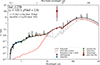 |
Fig. 2. SED of source lid_1278 (z = 3.013), one of the CTK AGN candidates in our sample. The colour-coded symbols show the observed photometry from CFHT-MegaCam (purple), Subaru-HSC (blue), VISTA (green), Spitzer/IRAC (orange), and Spitzer/MIPS (red). The solid black line indicates the best-fitting total model from CIGALE, decomposed into the AGN (disc + torus; dashed red line) and host-galaxy (stars + dust; dotted grey line) components. The predicted 6 μm flux derived from the X-ray luminosity is also shown (red cross). The best-fitting parameters are reported in the legend, including inclination angle and AGN fractional contribution. |
Best-fit model parameters from CIGALE SED fitting.
Our results are consistent with the presence of heavily obscured AGN. The high torus inclination angles indicate that the accretion disc emission is hidden in the optical regime. Although the Bayesian estimates for the AGN fraction are consistent with zero for some sources, visual inspection of the best-fitting SED models clearly shows that an AGN component is required to reproduce the observed 24 μm emission. The host-galaxy component alone cannot account for such high infrared fluxes, as also indicated by the non-zero “best” AGN fractions reported in Table 2. This is clearly illustrated in Fig. 2, where the optical part of the SED is dominated by the host galaxy (dotted grey line), whereas the rest-frame ∼3 − 30 μm range is clearly dominated by the AGN component (dashed red line).
Although the overall SED shapes support the CTK scenario, they do not, by themselves, provide strong constraints on the column density of these sources. In Sect. 3.2 below, we explore how the AGN luminosity at 6 μm, derived from our SED analysis, can be used to further investigate this aspect.
3.2. Constraining the X-ray absorption via the LX − L6 μm correlation
A well-established correlation exists between AGN emission in the X-ray and MIR regimes, particularly between the rest-frame 2−10 keV and 6 μm luminosities (e.g. Mateos et al. 2015; Stern 2015; Chen et al. 2017; Toba et al. 2019). This correlation arises from the shared origin of the two emissions: UV photons from the accretion disc serve as seed photons for Compton up-scattering in the X-ray corona, as well as for the thermal reprocessing by the circumnuclear dusty torus, which re-emits in the MIR. Owing to its robustness, this correlation has been used to identify heavily obscured AGNs (Alexander et al. 2008; Georgantopoulos et al. 2011; Severgnini et al. 2012; Carroll et al. 2021), and more recently, to place constraints on the line-of-sight NH via X-ray spectral modelling (Laloux et al. 2023).
In the left panel of Fig. 3, we present the rest-frame 2−10 keV luminosities derived from our X-ray spectral fits as a function of the rest-frame 6 μm luminosities obtained through SED modelling (Sect. 3.1) for the CTK candidates in our sample (coloured circles). For reference, we include a comparison sample of X-ray selected AGNs from the CCLS (black dots; Laloux et al. 2023). The distribution of our sources reveals a systematic offset above the Stern (2015) correlation (dashed black line), with the XXL-N and most CCLS sources lying beyond the 2σ dispersion (dashed gray lines) derived from the Laloux et al. (2023) sample.
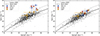 |
Fig. 3. Intrinsic X-ray luminosity in the 2−10 keV band versus the monochromatic 6 μm luminosity of the AGN component. The results for our CTK sample are shown before (left panel) and after (right panel) applying the IR luminosity prior, as described in Sect. 3.2. Grey dots represent the X-ray–selected AGN sample from Laloux et al. (2023) in the CCLS field. Large circles indicate our final CTK candidates, colour-coded by their parent X-ray survey: CDF (yellow), CCLS (red), XXL-N (blue). The dashed black line marks the LX − L6 μm relation from Stern (2015), while the dashed grey lines denote the 2σ dispersion of the Laloux et al. (2023) sample with respect to that relation. |
This discrepancy is further illustrated in Fig. 2, where we show the observed 6 μm flux inferred from the X-ray luminosities using the Stern (2015) relation (red cross). The expected IR flux is several orders of magnitude higher than what is predicted from our SED modelling, suggesting a significant overestimation of the X-ray luminosity. The availability of Spitzer/MIPS 24 μm imaging data for all CTK candidates provides a strong constraint on the rest-frame 6 μm emission at the redshift range of our sources, lending confidence to the reliability of the SED-derived IR luminosities.
The most plausible interpretation for the discrepancy is an overestimation of LX, driven by uncertainties in NH. Inspection of the NH posterior distributions (lower right panels of Figs. B.1–B.2) reveals that they are frequently broad or exhibit bimodal behaviour, with non-negligible posterior weight extending below the CTK threshold.
Figure 4 illustrates the joint posterior distribution in the log NH − log L6 μm plane (blue shaded region) for one of our CTK candidates, where L6 μm is computed from the LX posterior using the Stern (2015) relation. The distribution is characteristically bimodal, with a primary peak at high NH and high L6 μm, and a secondary peak at lower NH and correspondingly lower luminosity. Notably, the low-NH solution aligns well with the SED-inferred L6 μm value (black dashed line and gray shaded region), suggesting that the CTK classification may be driven by poorly constrained or degenerate NH estimates rather than robust spectral evidence.
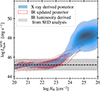 |
Fig. 4. Joint posterior distribution in the log NH − log L6 μm plane (shaded blue region) for source lid_1278, one of our CTK candidates. The IR luminosity L6 μm is inferred from the X-ray luminosity posterior via the Stern (2015) relation. The dashed black line and the shaded grey region show the SED-inferred L6 μm value and its uncertainty, while the red dotted contours indicate the posterior distribution after incorporating the IR prior. |
Laloux et al. (2023) demonstrated that the degeneracy in the log NH − log LX parameter space, commonly encountered in X-ray spectral fitting in the low-count regime, can be significantly reduced by incorporating IR luminosity constraints. In their approach, IR data are used to inform the X-ray spectral analysis through priors on the intrinsic X-ray luminosity, assuming a given LX − L6 μm correlation.
Following the same principle, we incorporate the constraints derived from our SED fitting into the X-ray analysis without re-performing the full spectral fit. Instead, we update the posterior probability distributions obtained with BXA using Bayes’ theorem:
 (1)
(1)
where P(z, log LX, log NH|X) is the original posterior distribution from the X-ray-only analysis, and 𝒩 is a Gaussian prior on log LX centred at the X-ray luminosity inferred from the SED-derived L6 μm (assuming the Stern 2015 correlation). The standard deviation σ of the prior is set to match the intrinsic scatter of the LX − L6 μm relation measured in the Laloux et al. (2023) sample. The updated posterior, P(z, log LX, log NH|X, IR), incorporates the additional IR constraint. This method is illustrated in Fig. 4, where the dotted red region represents the IR-informed posterior distribution.
We applied this approach to all CTK candidates in our sample. The right panel of Fig. 3 compares the updated LX values against the SED-inferred 6 μm luminosities. After incorporating the IR priors, the sources fall closer to the expected relation from Stern (2015), although a slight systematic overestimation of LX persists. Importantly, the updated posteriors have a significant impact on the inferred NH values. Figure 6 shows a comparison of the posterior probabilities of each source being CTK, obtained using the X-ray-only (grey bars) and IR-informed (red bars) posteriors. After applying the IR constraint, only three of the original CTK candidates show probabilities above our initial selection threshold of 80%.
This result highlights the critical importance of including IR data for the reliable identification of CTK sources. Figure 1 shows that a significant number of objects in the Pouliasis et al. (2024) sample exhibit nominal NH values above the CTK threshold but were excluded from our analysis due to low posterior probabilities of being CTK. These sources typically display broad NH posterior distributions, and therefore the inclusion of IR constraints could substantially refine their absorption estimates.
For a complete and unbiased characterisation of the CTK population–particularly in the context of high-redshift X-ray luminosity function studies (see Sect. 3.3)–it is essential to obtain IR luminosity estimates for the entire Pouliasis et al. (2024) sample. While a full SED analysis is beyond the scope of this work, we derived approximate L6 μm values using available MIR imaging.
All fields in the sample have been observed by Spitzer/MIPS at 24 μm, covering the majority of the survey areas. We retrieved the flux-calibrated MIPS mosaics from the SEIP database3 and performed aperture photometry at the optical counterpart positions of all sources in the Pouliasis et al. (2024) catalogue. This yielded observed 24 μm fluxes for the majority of sources. By adopting a representative AGN template from the CIGALE library, redshifting it appropriately, and scaling to the observed 24 μm flux, we estimated rest-frame L6 μm values. Using this method, we derived IR luminosity estimates for 574 out of 811 sources in the Pouliasis et al. (2024) sample. 236 sources in the XXL-N field lie outside the MIPS coverage, so we could not estimate IR luminosities for those sources.
These L6 μm values should be interpreted as upper limits, since we did not account for potential contamination from host galaxy emission or blending with nearby sources. To incorporate these estimates into the X-ray analysis, we updated the posterior distributions using a conservative prior on LX. Instead of a Gaussian, we used a step function prior: the probability is set to zero for  , and constant otherwise, where
  is the X-ray luminosity predicted from L6 μm using the Stern (2015) relation.
We checked this method by applying it to the ten CTK candidates for which we had SED-derived L6 μm values, and found that the two methods yield consistent results. We also tested the sensitivity of the outcome to the choice of AGN template, we recalculated the IR luminosities using an alternative AGN template and we verified that the specific template used had minimal impact on the final results, provided it corresponded to a high-inclination (edge-on) configuration.
Fig. 5 shows the impact of the IR-informed priors on the full Pouliasis et al. (2024) sample. The left and right panels display the stacked posterior distributions (Baronchelli et al. 2020, Appendix A) of NH and log LX, respectively. The black hatched histograms correspond to the original (X-ray-only) posteriors, while the red histograms reflect the IR-updated posteriors. While the overall LX distribution shows a modest shift towards lower luminosities, the effect on the NH distribution is more pronounced for the CTK population: the observed number density of CTK sources is reduced by approximately a factor of two. The distributions for unabsorbed and Compton-thin sources remain largely unaffected.
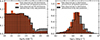 |
Fig. 5. Observed distributions of hydrogen column density and X-ray luminosity for the full Pouliasis et al. (2024) sample. The black-hatched histograms show the original X-ray posteriors, while the solid red histograms correspond to the posteriors updated with IR information (see Sect. 3.2). |
3.3. X-ray luminosity function for CTK AGNs
The XLF of AGNs is a fundamental diagnostic of black hole growth and AGN evolution (Fotopoulou et al. 2016). By tracing the number density of AGNs as a function of luminosity and redshift, the XLF provides a robust observational constraint of accretion activity across cosmic time (Aird et al. 2015a). An additional dimension can be introduced by including the hydrogen column density, NH, which enables the study of the cosmic evolution of the intrinsic AGN population as a function of X-ray absorption. This leads to the definition of the XLAF:
 (2)
(2)
where the XLAF, ϕabs(LX, NH, z), represents the number of sources N per unit comoving volume V, per logarithmic interval in luminosity and column density, as a function of LX, NH and z. It is commonly assumed that the XLAF can be factorised into two components (e.g. Ueda et al. 2003, 2014; Vijarnwannaluk et al. 2022): the XLF, ϕ(LX, z), and the absorption function, fabs(NH, LX, z).
In this work, we follow the methodology of Pouliasis et al. (2024) to derive a parametric form of the XLAF for CTK sources in the redshift range z = 3 − 6. The XLF is parametrised as a broken power law (Barger et al. 2005) with pure density evolution (PDE; Schmidt 1968). Pouliasis et al. (2024) tested various evolutionary models for the XLF, finding no statistically significant differences among them when applied to our dataset. We adopt the PDE model here, as it offers a good description of the data with the fewest free parameters.
For the absorption function, we use the parametrisation from Pouliasis et al. (2024): a flat-step function defined over three NH intervals, with values that depend on both redshift and X-ray luminosity. A detailed description of the XLAF parametrisation is provided in Appendix A.
As in Pouliasis et al. (2024), we employ a Bayesian inference framework to estimate simultaneously the parametric forms of the XLF and absorption function. This approach allows a rigorous propagation of the uncertainties in the X-ray spectral parameters and photometric redshifts of individual sources, encoded in their posterior probability distributions. The posterior distribution of the XLAF parameters is sampled using MLFriends (Buchner 2016; Buchner & Bauer 2017), a nested-sampling Monte Carlo algorithm implemented in the UltraNest package. Full details of the methodology are given in Appendix A.
In addition to the parametric modelling described above, we derived a binned representation of the XLAF using the method of Miyaji et al. (2001). This approach estimates the space density in each luminosity, NH and redshift bin by scaling the analytical XLAF model according to the ratio of the observed to predicted number of sources,
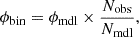 (3)
(3)
where Nobs is the number of detected sources and Nmdl is the number expected from ϕmdl, the best-fitting XLAF model within the same bin, obtained by integrating the model over the survey sensitivity function. This method preserves the overall shape of the parametric model while providing a data-driven visualisation of the luminosity function. The uncertainties in each bin are computed assuming Poisson statistics.
Figure 7 presents our final XLAF estimates for two redshift intervals (z = 3 − 4 and z = 4 − 6) and two column density ranges (log NH = 20 − 24 and log NH = 24 − 26). Solid black lines and shaded grey regions show the median and 1σ uncertainty of the XLAF derived using X-ray data alone, while red lines and the corresponding shaded regions show the results obtained after including the IR-updated posteriors. In the unabsorbed and Compton-thin regimes, the results are consistent, both exhibiting similar XLF shapes, confirming the robustness of the Pouliasis et al. (2024) results. In contrast, the CTK regime shows a systematic shift towards lower space densities when the IR information is included; an expected outcome given that, as shown in Sect. 3.2, the number of CTK sources is reduced by approximately half once the IR constraints are applied (see also Fig. 5).
The derived XLAF can also be used to estimate the intrinsic fraction of CTK AGNs within our redshift range of interest. This fraction is defined as
 (4)
(4)
where N represents the number of sources within the specified comoving volume and column density range, obtained by integrating the XLAF over the relevant intervals in redshift, luminosity, and NH. From our best-fitting XLAF model, we find an intrinsic CTK fraction of  in the redshift range z = 3 − 6. A comparison of this estimate with previous results will be discussed in Sect. 4.
4. Discussion
4.1. Reliability of NH estimates
A reasonable concern is whether XMM-Newton and Chandra that operate in a relatively soft energy band below 10 keV, can efficiently detect CTK AGNs. Indeed, extending the energy range of the X-ray spectra above 10 keV e.g. using NuSTAR can provide accurate column density estimates especially at low redshifts (e.g. Ricci et al. 2015). However, at the redshift range explored in this work the energy turnovers due to the mild CTK absorption are expected to lie at energies above 1.5 keV. These energies are where the effective area of XMM-Newton and Chandra is the highest. Furthermore, NuSTAR is not sensitive enough to detect sources in the redshift range we explore in this paper. For example, Aird et al. (2015a) compiled a sample of 94 sources using the NuSTAR extragalactic survey program (Harrison et al. 2013) and estimated the AGN XLF. No radio-quiet AGNs have been detected above a redshift of z = 3. Moreover, Tokayer et al. (2025) caution that XMM-Newton and Chandra spectral fits using a limited number of counts are reliable especially in the case of CTK AGNs. As already mentioned above, Laloux et al. (2023) attempt to limit the effect of this constraint by employing MIR priors.
In Sect. 3 we examined the reliability of the X-ray–derived absorption estimates for our sample of CTK AGN candidates. By combining the X-ray spectral results with multiwavelength information, in particular the IR constraints derived from SED fitting, we evaluated how robustly the X-ray data alone can identify genuine CTK sources across surveys of varying depth. As discussed in Sect. 3.2, the number of CTK candidates in our sample decreases from ten to three once their multiwavelength properties are examined in detail. In most cases, the derived column densities remain indicative of a heavily obscured environment, although they fall below the formal CTK threshold. This suggests that while strong absorption is present, the extreme levels implied by the initial X-ray analysis are not always robust.
The impact of introducing IR information varies across surveys. This effect is illustrated in Fig. 6 where we show the probabilities of our selected CTK candidates of having log NH > 24 derived from the corresponding posteriors before and after updating with the IR information. Sources in the Chandra Deep Fields are the least affected, owing to the significantly longer exposure times in these regions. Their spectra typically contain more than 100 net counts, allowing for a reliable detection of the Fe Kα emission line expected in CTK AGNs (George & Fabian 1991) and providing well-constrained estimates of NH based solely on the X-ray data.
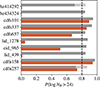 |
Fig. 6. Probability that the selected CTK candidates have log NH > 24. Grey bars show the original probabilities estimated using the X-ray only posteriors, and red bars show the results using the IR-updated posteriors. Light grey areas show the estimated probabilities before applying the redshift corrections discussed in Sect. 2.1. The vertical dashed black line shows our initial selection criterion for the CTK sample. |
In contrast, the CTK candidates identified in the shallower CCLS and XXL-N surveys have much lower-count spectra, often containing only a few tens of counts. While the overall continuum shape in these cases is consistent with high absorption, the inferred NH values are considerably less secure. In such low signal-to-noise regimes, apparent CTK classifications can be driven by Poisson fluctuations near the observed energy of the Fe Kα line rather than by genuine spectral features.
These results highlight that only high signal-to-noise X-ray observations can reliably constrain NH in the CTK regime at these redshifts. For the majority of current XMM-Newton and Chandra surveys, the available depth is insufficient for a robust identification of CTK sources at high redshift based on X-ray data alone. Incorporating complementary IR information is therefore essential to obtain a reliable census of the most heavily obscured AGNs.
4.2. The CTK AGN luminosity function
Section 3.3 presented our estimates of the XLF for the high-redshift CTK AGN population. In that analysis, we tested the impact of incorporating IR–updated priors into the X-ray spectral fitting results. The inclusion of IR information systematically shifts the inferred space densities towards lower values, reflecting a more conservative and physically consistent view of the CTK population. The discussion that follows refers exclusively to these IR-updated results.
The binned luminosity function (Fig. 7) shows that our data provide meaningful constraints on the CTK population only within the z = 3 − 4 redshift interval and over the luminosity range 43.5 ≤ log LX ≤ 45. At lower luminosities, the CTK population remains essentially unconstrained, as the current surveys lack the sensitivity required to reliably detect CTK sources below log LX ∼ 43 at these redshifts. Similarly, for z = 4 − 6, the XLF is constrained only by upper limits, indicating that the available data are insufficient to fully characterise the evolution of the most heavily obscured AGNs at these epochs.
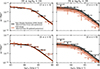 |
Fig. 7. XLAF for two redshift intervals (z = 3 − 4, top panels; z = 4 − 6, bottom panels) and two hydrogen column density ranges (log NH = 20 − 24, left panels; log NH = 24 − 26, right panels). Black lines and grey shaded regions indicate the results for the parametric XLAF obtained from the X-ray-only posteriors, while red lines and shaded regions correspond to those derived using the IR luminosity priors. The corresponding binned XLAFs were derived using the Miyaji et al. (2001) method. |
It should also be noted that the Pouliasis et al. (2024) sample is selected in the soft X-ray band (0.5−2 keV). At the redshifts considered here, this energy range approximately corresponds to the rest-frame hard band (2−10 keV), which may lead to the exclusion of the most extremely obscured, reflection-dominated CTK sources. Indeed, our sample does not include some known high-z CTK AGNs, such as the z = 4.762 source in the CDF-S reported by Gilli et al. (2014). These selection effects should be kept in mind when interpreting our results, as they imply that our parametric estimates of the XLAF rely partly on extrapolations in luminosity and redshift regimes where direct observational constraints are limited.
Figure 8 presents our final CTK XLF for z = 3 − 6, compared with previous studies. We include the high-redshift CTK XLFs of Buchner et al. (2015) and Aird et al. (2015b), as well as the local (z < 0.05) CTK XLF derived by Georgantopoulos et al. (2025). The latter was obtained from a Swift/BAT-selected sample of local AGNs, with NH values measured using NuSTAR observations. The high-z studies by Buchner et al. (2015) and Aird et al. (2015b) were selected because they are based on X-ray surveys similar to ours–combining deep, pencil-beam observations with shallower, wide-area fields (using Chandra and XMM-Newton observations)–and employ comparable Bayesian methodologies to infer the luminosity function. The principal distinction lies in their functional forms: Buchner et al. (2015) adopted a non-parametric approach, whereas Aird et al. (2015b) employed a parametric model. The latter, a flexible double power-law formulation, allows all parameters of the double power law to evolve as polynomial functions of log(1 + z), thereby accommodating redshift-dependent variations in the XLF shape driven by the data. We also compared with the XLAF of (Ananna et al. 2019). This luminosity function is derived from a population synthesis model aiming to reproduce the Cosmic X-ray Background and the observed counts of CTK-AGNs in surveys with XMM-Newton, Chandra, NuSTAR and Swift/BAT.
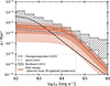 |
Fig. 8. XLF for the CTK population (24 < log NH < 26). Red symbols show our result for the parametric XLF in the 3−6 redshift range. The solid red line corresponds to the median value and shaded areas are the 1σ (darker red) and 2σ (lighter red) uncertainties. The dashed black line is the XLF for CTK sources in the local universe (z < 0.05) derived by Georgantopoulos et al. (2025). The grey-hatched area is the non-parametric XLF in the 3.1−7 redshift range estimated by Buchner et al. (2015). The area shows the 90% confidence region. The dotted blue line corresponds to the Aird et al. (2015b) XLF for CTK AGNs in the 3−6 redshift range. |
Our results are consistent with Aird et al. (2015b) and systematically lower than those reported by Buchner et al. (2015). When compared to the local Universe, our XLF indicates a substantially lower space density of CTK sources at low luminosities (log LX < 43), while all studies show an increasing density towards higher luminosities (log LX > 44). Interestingly, the local XLF of Georgantopoulos et al. (2025) aligns closely with the low-luminosity end of the Buchner et al. (2015) results.
The discrepancy between our results and those of Buchner et al. (2015) may stem from methodological differences. Their analysis relied solely on X-ray data, without the benefit of IR constraints, which, as we have shown, tend to reduce the inferred CTK number densities. However, the consistency between our IR-informed results and those of Aird et al. (2015b), which were also based exclusively on X-ray data, suggests that additional factors are at play. A key distinction is that Buchner et al. (2015) derived individual source properties through full spectral modelling, similar to our approach, whereas Aird et al. (2015b) employed broadband count-rate analyses. It is likely that the latter method is less prone to spurious identification of CTK sources, as it does not rely on detailed spectral features, such as the Fe Kα line, that can be affected by low-count statistical fluctuations.
Overall, our results suggest that the space density of CTK AGNs at z = 3 − 6 is lower than previously inferred from X-ray data alone, although the uncertainties remain substantial due to limited statistics and selection biases. The consistency between our IR-informed analysis and independent parametric estimates reinforces the robustness of our approach, while also highlighting the need for deeper, high-energy observations–such as those anticipated from NewAthena and other future missions–to fully characterise the obscured growth of SMBHs in the early Universe.
4.3. The evolution of the CTK fraction
Figure 9 compares our estimates of the CTK fraction4 in the redshift range z = 3 − 6 with previous measurements spanning from the local Universe up to z ∼ 6. The results from Buchner et al. (2015) and Aird et al. (2015b) are derived from the luminosity functions presented in Sect. 4.2. The estimates of Lanzuisi et al. (2018) are based on a study of CTK AGNs selected in the CCLS, while those of Laloux et al. (2023) also rely on CCLS data but employ a non-parametric approach to model the XLAF of the AGN population. In Laloux et al. (2023), X-ray spectral fitting was performed for individual sources using IR–derived priors. The measurement by Masini et al. (2018) originates from a NuSTAR survey of the UKIDSS Ultra Deep Survey field and represents the observed CTK fraction, which can be considered a lower limit to the intrinsic value. For comparison, we also include two estimates of the CTK fraction for the local Universe from Burlon et al. (2011) and Georgantopoulos et al. (2025). Additionally, we have incorporated the CTK fractions estimated through the integration of the luminosity function estimated by Ananna et al. (2019). We calculated the CTK fraction across two different NH intervals (24 ≤ log NH ≤ 25, and 24 ≤ log NH ≤ 26).
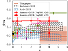 |
Fig. 9. Evolution of the fraction of CTK sources over the total AGN population across redshift. Our results are shown with the red shaded regions, which represent the 1σ (darker red) and 2σ (lighter red) confidence regions. The grey-hatched area corresponds to the Buchner et al. (2015) results (90% confidence interval) for AGNs in the 43.2 ≤ log LX ≤ 43.6 interval. The blue-hatched area shows the Aird et al. (2015b) estimates (99% confidence interval) for sources with log LX = 43.5. The green squares show the Laloux et al. (2023) results; quoted upper limits are 3σ. Pink triangles correspond to the results by Lanzuisi et al. (2018) and purple diamond corresponds to a study by Masini et al. (2018). The black (Georgantopoulos et al. 2025) and yellow (Burlon et al. 2011) circles show the CTK fraction in the local Universe using Swift/BAT selected AGNs. Red diamonds show the fraction of CTK sources estimated through the integration of the Ananna et al. (2019) luminosity function. Open symbols show the result in the range (24 ≤ log NH < 26), while filled symbols are for (24 ≤ log NH < 25). |
Among these studies, the results of Buchner et al. (2015) and Lanzuisi et al. (2018) stand out for their remarkably high CTK fraction of approximately 40−50%, among the largest values reported in the literature at high redshift. Such high fractions are, however, in clear tension with both our findings and those of other works. For example, Aird et al. (2015b) reported lower CTK fractions that are broadly consistent with our results in the z = 3 − 6 range, although they noted that their highest-redshift bins may be affected by limited statistics. The results of Ananna et al. (2019) show no evolution with redshift and, for the population with log NH < 25, the CTK fraction is about 30 per cent, consistent with previous results in similar redshift ranges. The estimate for the high redshift range (3 < z < 5) aligns with our estimate of the CTK fraction at high redshifts. However, when considering the population with log NH > 25, the CTK fraction from Ananna et al. (2019) reaches ∼50% that is similar to the highest values reported in the literature (Lanzuisi et al. 2018). This discrepancy may arise from the limited sensitivity to this highly absorbed population in the X-ray energies examined by these studies.
At intermediate redshifts (0.5 < z < 2.5), most studies converge on a CTK fraction of 15−30%, consistent with estimates for the local Universe. Overall, the emerging picture suggests no compelling evidence of a strong evolution of the CTK fraction up to z ≈ 5 − 6. The only study reporting a significant increase is that of Lanzuisi et al. (2018), who found a rise from ∼20% at low redshift to nearly 50% at z ∼ 3. These results appear to be in tension with the more recent analysis by Laloux et al. (2023) of the same field, whose upper limits around z ∼ 3 favour a lower CTK fraction than that inferred by Lanzuisi et al. (2018).
In contrast, the evolution of the total obscured AGN population (including Compton-thin sources) is well established (e.g. Vito et al. 2018; Signorini et al. 2023; Peca et al. 2023; Pouliasis et al. 2024), showing a pronounced increase towards higher redshifts. This trend may be explained by the findings of Gilli et al. (2022), who proposed that the rise in the obscured AGN population is primarily linked to the interstellar medium (ISM) of the host galaxies. Their model suggests that ISM-driven obscuration rarely reaches the CTK regime at these redshifts. Instead, the ISM is expected to dominate obscuration within the Compton-thin range, while the relative contribution of CTK sources remains approximately constant across cosmic time.
These findings support a scenario in which the most heavily obscured, CTK phase of AGN activity represents a relatively stable component of black hole growth. The strong redshift evolution observed in the overall obscured population is therefore likely driven by increasing Compton-thin obscuration associated with the evolving ISM of high-redshift galaxies (Scoville et al. 2014, 2017).
5. Conclusions
We investigated the population of CTK AGNs at high redshifts (z ≥ 3) using the Pouliasis et al. (2024) sample, one of the largest X-ray–selected AGN datasets currently available in this regime. From this sample, we identified a subsample of ten high-probability CTK candidates based on the Bayesian X-ray spectral fits of Pouliasis et al. (2024) and examined their multiwavelength properties through SED analysis to assess the robustness of their CTK classifications. While the SEDs are generally consistent with heavily obscured AGN, a substantial fraction of the sources exhibit X-ray luminosities significantly higher than expected from the established correlations between LX and L6 μm. Most of these outliers have low-count X-ray spectra, suggesting that the discrepancy arises from an overestimate of NH.
To address this, we applied the methodology of Laloux et al. (2023) to update the X-ray posterior distributions with the IR constraints derived from our SED analysis. This yielded more physically consistent X-ray properties. After this update, only three sources retained a high probability of being CTK; the others still showed substantial absorption but below the nominal CTK threshold.
We then derived the XLF for CTK AGNs in parametric form, using the complete sample and methodology of Pouliasis et al. (2024). The individual X-ray posteriors were updated using L6 μm upper limits estimated from Spitzer/MIPS 24 μm photometry to obtain more robust values for LX and NH. Incorporating IR constraints systematically reduces the inferred space density of CTK AGNs, resulting in a more conservative and physically consistent description of the population, while leaving the unabsorbed and Compton-thin XLF largely unaffected. The resulting CTK XLF provides meaningful constraints for z = 3 − 4 and 43.5 ≲ log LX ≲ 45, whereas at lower luminosities and higher redshifts the data remain limited by current survey sensitivities.
Our derived CTK XLF is consistent with that of Aird et al. (2015b) and lower than the estimates of Buchner et al. (2015), underscoring the importance of multiwavelength constraints in mitigating degeneracies in X-ray spectral fitting. We find an intrinsic CTK fraction of  in the redshift range z = 3 − 6. Comparisons with local and intermediate-redshift measurements indicate that the CTK space density remains broadly stable with redshift, in contrast to the overall obscured AGN population (including Compton-thin sources), which shows strong evolution towards higher redshifts. This trend likely reflects increasing ISM in high-redshift galaxies, while the intrinsic CTK fraction remains approximately constant across cosmic time.
Overall, our results support a scenario in which the CTK phase represents a persistent but relatively rare mode of black hole growth, contributing a stable fraction to the accretion history of the Universe. Future high-sensitivity, broadband X-ray observatories such as NewAthena and HEX-P will be essential to further constrainining this population, extending current analyses to lower luminosities and providing a more robust census of the most heavily obscured AGNs at early cosmic epochs.
Acknowledgments
The research leading to these results has received funding from the Hellenic Foundation for Research and Innovation (HFRI) project “4MOVE-U” grant agreement 2688, which is part of the programme “2nd Call for HFRI Research Projects to support Faculty Members and Researchers”. EP and IG acknowledge ACME, a project funded by the European Union’s Horizon Europe Research and Innovation programme under Grant Agreement 101131928. Based on observations obtained with XMM-Newton, an ESA science mission with instruments and contributions directly funded by ESA member states and NASA. This research has made use of data obtained from the Chandra Data Archive and the Chandra Source Catalogue, and software provided by the Chandra X-ray Center (CXC) in the application packages CIAO and Sherpa. This research has made use of the NASA/IPAC Infrared Science Archive, which is funded by the National Aeronautics and Space Administration and operated by the California Institute of Technology. This work is based on observations made with the Spitzer Space Telescope, which is operated by the Jet Propulsion Laboratory, California Institute of Technology under a contract with NASA. This work made use of Astropy (http://www.astropy.org): a community-developed core Python package and an ecosystem of tools and resources for astronomy (Astropy Collaboration 2013, 2018, 2022). The plots in this publication were produced using Matplotlib, a Python library for publication-quality graphics (Hunter 2007).
References
- Aird, J., Alexander, D. M., Ballantyne, D. R., et al. 2015a, ApJ, 815, 66 [NASA ADS] [CrossRef] [Google Scholar]
- Aird, J., Coil, A. L., Georgakakis, A., et al. 2015b, MNRAS, 451, 1892 [Google Scholar]
- Akylas, A., Georgakakis, A., Georgantopoulos, I., Brightman, M., & Nandra, K. 2012, A&A, 546, A98 [NASA ADS] [CrossRef] [EDP Sciences] [Google Scholar]
- Akylas, A., Georgantopoulos, I., Ranalli, P., et al. 2016, A&A, 594, A73 [NASA ADS] [CrossRef] [EDP Sciences] [Google Scholar]
- Akylas, A., Georgantopoulos, I., Gandhi, P., Boorman, P., & Greenwell, C. L. 2024, A&A, 692, A250 [NASA ADS] [CrossRef] [EDP Sciences] [Google Scholar]
- Alexander, D. M., & Hickox, R. C. 2012, New Astron. Rev., 56, 93 [Google Scholar]
- Alexander, D. M., Chary, R. R., Pope, A., et al. 2008, ApJ, 687, 835 [NASA ADS] [CrossRef] [Google Scholar]
- Ananna, T. T., Treister, E., Urry, C. M., et al. 2019, ApJ, 871, 240 [Google Scholar]
- Annuar, A., Alexander, D. M., Gandhi, P., et al. 2025, MNRAS, 540, 3827 [Google Scholar]
- Antonucci, R. R. J., & Miller, J. S. 1985, ApJ, 297, 621 [NASA ADS] [CrossRef] [Google Scholar]
- Ashby, M. L. N., Stanford, S. A., Brodwin, M., et al. 2013, ApJS, 209, 22 [NASA ADS] [CrossRef] [Google Scholar]
- Astropy Collaboration (Robitaille, T. P., et al.) 2013, A&A, 558, A33 [NASA ADS] [CrossRef] [EDP Sciences] [Google Scholar]
- Astropy Collaboration (Price-Whelan, A. M., et al.) 2018, AJ, 156, 123 [Google Scholar]
- Astropy Collaboration (Price-Whelan, A. M., et al.) 2022, ApJ, 935, 167 [NASA ADS] [CrossRef] [Google Scholar]
- Barger, A. J., Cowie, L. L., Mushotzky, R. F., et al. 2005, AJ, 129, 578 [NASA ADS] [CrossRef] [Google Scholar]
- Baronchelli, L., Nandra, K., & Buchner, J. 2020, MNRAS, 498, 5284 [NASA ADS] [CrossRef] [Google Scholar]
- Barthelmy, S. D., Barbier, L. M., Cummings, J. R., et al. 2005, Space Sci. Rev., 120, 143 [Google Scholar]
- Boorman, P. G., Gandhi, P., Buchner, J., et al. 2025, ApJ, 978, 118 [Google Scholar]
- Boquien, M., Burgarella, D., Roehlly, Y., et al. 2019, A&A, 622, A103 [NASA ADS] [CrossRef] [EDP Sciences] [Google Scholar]
- Brandt, W. N., & Alexander, D. M. 2015, A&ARv, 23, 1 [Google Scholar]
- Brightman, M., Nandra, K., Salvato, M., et al. 2014, MNRAS, 443, 1999 [NASA ADS] [CrossRef] [Google Scholar]
- Bruzual, G., & Charlot, S. 2003, MNRAS, 344, 1000 [NASA ADS] [CrossRef] [Google Scholar]
- Buchner, J. 2016, Stat. Comput., 26, 383 [Google Scholar]
- Buchner, J. 2021, J. Open Source Softw., 6, 3001 [CrossRef] [Google Scholar]
- Buchner, J., & Bauer, F. E. 2017, MNRAS, 465, 4348 [Google Scholar]
- Buchner, J., Georgakakis, A., Nandra, K., et al. 2014, A&A, 564, A125 [NASA ADS] [CrossRef] [EDP Sciences] [Google Scholar]
- Buchner, J., Georgakakis, A., Nandra, K., et al. 2015, ApJ, 802, 89 [Google Scholar]
- Buchner, J., Brightman, M., Nandra, K., Nikutta, R., & Bauer, F. E. 2019, A&A, 629, A16 [NASA ADS] [CrossRef] [EDP Sciences] [Google Scholar]
- Burlon, D., Ajello, M., Greiner, J., et al. 2011, ApJ, 728, 58 [Google Scholar]
- Carroll, C. M., Hickox, R. C., Masini, A., et al. 2021, ApJ, 908, 185 [NASA ADS] [CrossRef] [Google Scholar]
- Charlot, S., & Fall, S. M. 2000, ApJ, 539, 718 [Google Scholar]
- Chen, C.-T. J., Hickox, R. C., Goulding, A. D., et al. 2017, ApJ, 837, 145 [Google Scholar]
- Civano, F., Marchesi, S., Comastri, A., et al. 2016, ApJ, 819, 62 [Google Scholar]
- Comastri, A., Setti, G., Zamorani, G., & Hasinger, G. 1995, A&A, 296, 1 [NASA ADS] [Google Scholar]
- Dale, D. A., Helou, G., Magdis, G. E., et al. 2014, ApJ, 784, 83 [Google Scholar]
- Edge, A., Sutherland, W., Kuijken, K., et al. 2013, The Messenger, 154, 32 [NASA ADS] [Google Scholar]
- Fotopoulou, S., Buchner, J., Georgantopoulos, I., et al. 2016, A&A, 587, A142 [NASA ADS] [CrossRef] [EDP Sciences] [Google Scholar]
- García-Burillo, S., Combes, F., Ramos Almeida, C., et al. 2016, ApJ, 823, L12 [Google Scholar]
- Georgakakis, A., Aird, J., Buchner, J., et al. 2015, MNRAS, 453, 1946 [Google Scholar]
- Georgakakis, A., Salvato, M., Liu, Z., et al. 2017, MNRAS, 469, 3232 [NASA ADS] [CrossRef] [Google Scholar]
- Georgantopoulos, I., & Akylas, A. 2019, A&A, 621, A28 [NASA ADS] [CrossRef] [EDP Sciences] [Google Scholar]
- Georgantopoulos, I., Rovilos, E., Akylas, A., et al. 2011, A&A, 534, A23 [NASA ADS] [CrossRef] [EDP Sciences] [Google Scholar]
- Georgantopoulos, I., Comastri, A., Vignali, C., et al. 2013, A&A, 555, A43 [NASA ADS] [CrossRef] [EDP Sciences] [Google Scholar]
- Georgantopoulos, I., Pouliasis, E., Ruiz, A., & Akylas, A. 2025, A&A, 695, A128 [NASA ADS] [CrossRef] [EDP Sciences] [Google Scholar]
- George, I. M., & Fabian, A. C. 1991, MNRAS, 249, 352 [Google Scholar]
- Giavalisco, M., Ferguson, H. C., Koekemoer, A. M., et al. 2004, ApJ, 600, L93 [NASA ADS] [CrossRef] [Google Scholar]
- Gilli, R., Comastri, A., & Hasinger, G. 2007, A&A, 463, 79 [NASA ADS] [CrossRef] [EDP Sciences] [Google Scholar]
- Gilli, R., Norman, C., Vignali, C., et al. 2014, A&A, 562, A67 [NASA ADS] [CrossRef] [EDP Sciences] [Google Scholar]
- Gilli, R., Norman, C., Calura, F., et al. 2022, A&A, 666, A17 [NASA ADS] [CrossRef] [EDP Sciences] [Google Scholar]
- Grogin, N. A., Kocevski, D. D., Faber, S. M., et al. 2011, ApJS, 197, 35 [NASA ADS] [CrossRef] [Google Scholar]
- Haardt, F., & Maraschi, L. 1991, ApJ, 380, L51 [Google Scholar]
- Harrison, F. A., Craig, W. W., Christensen, F. E., et al. 2013, ApJ, 770, 103 [Google Scholar]
- Hasinger, G., Miyaji, T., & Schmidt, M. 2005, A&A, 441, 417 [NASA ADS] [CrossRef] [EDP Sciences] [Google Scholar]
- Hönig, S. F., Kishimoto, M., Antonucci, R., et al. 2012, ApJ, 755, 149 [CrossRef] [Google Scholar]
- Hunter, J. D. 2007, Comput. Sci. Eng., 9, 90 [NASA ADS] [CrossRef] [Google Scholar]
- IRSA& SSC 2020, Spitzer Enhanced Imaging Products, NASA IPAC DataSet, IRSA433 [Google Scholar]
- Jarvis, M. J., Bonfield, D. G., Bruce, V. A., et al. 2013, MNRAS, 428, 1281 [Google Scholar]
- Kloek, T., & van Dijk, H. K. 1978, Econometrica, 46, 1 [CrossRef] [Google Scholar]
- Koekemoer, A. M., Faber, S. M., Ferguson, H. C., et al. 2011, ApJS, 197, 36 [NASA ADS] [CrossRef] [Google Scholar]
- Komatsu, E., Dunkley, J., Nolta, M. R., et al. 2009, ApJS, 180, 330 [NASA ADS] [CrossRef] [Google Scholar]
- Laloux, B., Georgakakis, A., Andonie, C., et al. 2023, MNRAS, 518, 2546 [Google Scholar]
- Lanzuisi, G., Ranalli, P., Georgantopoulos, I., et al. 2015, A&A, 573, A137 [NASA ADS] [CrossRef] [EDP Sciences] [Google Scholar]
- Lanzuisi, G., Civano, F., Marchesi, S., et al. 2018, MNRAS, 480, 2578 [Google Scholar]
- Lawrence, A., Warren, S. J., Almaini, O., et al. 2007, MNRAS, 379, 1599 [Google Scholar]
- Loredo, T. J. 2004, AIP Conf. Ser., 735, 195 [NASA ADS] [CrossRef] [Google Scholar]
- Luo, B., Brandt, W. N., Xue, Y. Q., et al. 2017, ApJS, 228, 2 [Google Scholar]
- Lynden-Bell, D. 1969, Nature, 223, 690 [NASA ADS] [CrossRef] [Google Scholar]
- Marchesi, S., Civano, F., Elvis, M., et al. 2016, ApJ, 817, 34 [Google Scholar]
- Masini, A., Civano, F., Comastri, A., et al. 2018, ApJS, 235, 17 [Google Scholar]
- Mateos, S., Carrera, F. J., Alonso-Herrero, A., et al. 2015, MNRAS, 449, 1422 [Google Scholar]
- McMahon, R. G., Banerji, M., Gonzalez, E., et al. 2013, The Messenger, 154, 35 [NASA ADS] [Google Scholar]
- Miyaji, T., Hasinger, G., & Schmidt, M. 2000, A&A, 353, 25 [NASA ADS] [Google Scholar]
- Miyaji, T., Hasinger, G., & Schmidt, M. 2001, A&A, 369, 49 [NASA ADS] [CrossRef] [EDP Sciences] [Google Scholar]
- Miyaji, T., Hasinger, G., Salvato, M., et al. 2015, ApJ, 804, 104 [Google Scholar]
- Miyazaki, S., Komiyama, Y., Kawanomoto, S., et al. 2018, PASJ, 70, S1 [NASA ADS] [Google Scholar]
- Nenkova, M., Sirocky, M. M., Ivezić, Ž., & Elitzur, M. 2008a, ApJ, 685, 147 [Google Scholar]
- Nenkova, M., Sirocky, M. M., Nikutta, R., Ivezić, Ž., & Elitzur, M. 2008b, ApJ, 685, 160 [Google Scholar]
- Netzer, H. 2015, ARA&A, 53, 365 [Google Scholar]
- Peca, A., Cappelluti, N., Urry, C. M., et al. 2023, ApJ, 943, 162 [NASA ADS] [CrossRef] [Google Scholar]
- Pierre, M., Pacaud, F., Adami, C., et al. 2016, A&A, 592, A1 [NASA ADS] [CrossRef] [EDP Sciences] [Google Scholar]
- Pouliasis, E., Mountrichas, G., Georgantopoulos, I., et al. 2022, A&A, 667, A56 [NASA ADS] [CrossRef] [EDP Sciences] [Google Scholar]
- Pouliasis, E., Ruiz, A., Georgantopoulos, I., et al. 2024, A&A, 685, A97 [NASA ADS] [CrossRef] [EDP Sciences] [Google Scholar]
- Press, W. H., Teukolsky, S. A., Vetterling, W. T., & Flannery, B. F. 2007, Numerical Recipes: The Art of Scientific Computing (Cambridge: Cambridge University Press) [Google Scholar]
- Ricci, C., Ueda, Y., Koss, M. J., et al. 2015, ApJ, 815, L13 [Google Scholar]
- Sajina, A., Lacy, M., & Pope, A. 2022, Universe, 8, 356 [NASA ADS] [CrossRef] [Google Scholar]
- Salpeter, E. E. 1955, ApJ, 121, 161 [Google Scholar]
- Sawicki, M., Arnouts, S., Huang, J., et al. 2019, MNRAS, 489, 5202 [NASA ADS] [Google Scholar]
- Schartmann, M., Meisenheimer, K., Camenzind, M., Wolf, S., & Henning, T. 2005, A&A, 437, 861 [NASA ADS] [CrossRef] [EDP Sciences] [Google Scholar]
- Schmidt, M. 1968, ApJ, 151, 393 [Google Scholar]
- Scoville, N., Aussel, H., Sheth, K., et al. 2014, ApJ, 783, 84 [CrossRef] [Google Scholar]
- Scoville, N., Lee, N., Vanden Bout, P., et al. 2017, ApJ, 837, 150 [Google Scholar]
- Severgnini, P., Caccianiga, A., & Della Ceca, R. 2012, A&A, 542, A46 [NASA ADS] [CrossRef] [EDP Sciences] [Google Scholar]
- Shirley, R., Duncan, K., Campos Varillas, M. C., et al. 2021, MNRAS, 507, 129 [NASA ADS] [CrossRef] [Google Scholar]
- Signorini, M., Marchesi, S., Gilli, R., et al. 2023, A&A, 676, A49 [NASA ADS] [CrossRef] [EDP Sciences] [Google Scholar]
- Stalevski, M., Fritz, J., Baes, M., Nakos, T., & Popović, L. Č. 2012, MNRAS, 420, 2756 [Google Scholar]
- Stalevski, M., Ricci, C., Ueda, Y., et al. 2016, MNRAS, 458, 2288 [Google Scholar]
- Stern, D. 2015, ApJ, 807, 129 [Google Scholar]
- Straatman, C. M. S., Spitler, L. R., Quadri, R. F., et al. 2016, ApJ, 830, 51 [NASA ADS] [CrossRef] [Google Scholar]
- Toba, Y., Ueda, Y., Matsuoka, K., et al. 2019, MNRAS, 484, 196 [Google Scholar]
- Tokayer, Y. M., Koss, M. J., Urry, C. M., et al. 2025, ApJ, 982, 134 [Google Scholar]
- Torres-Albà, N., Marchesi, S., Zhao, X., et al. 2021, ApJ, 922, 252 [CrossRef] [Google Scholar]
- Ueda, Y., Akiyama, M., Ohta, K., & Miyaji, T. 2003, ApJ, 598, 886 [NASA ADS] [CrossRef] [Google Scholar]
- Ueda, Y., Akiyama, M., Hasinger, G., Miyaji, T., & Watson, M. G. 2014, ApJ, 786, 104 [Google Scholar]
- Vijarnwannaluk, B., Akiyama, M., Schramm, M., et al. 2022, ApJ, 941, 97 [NASA ADS] [CrossRef] [Google Scholar]
- Vijarnwannaluk, B., Akiyama, M., Schramm, M., et al. 2024, MNRAS, 529, 3610 [Google Scholar]
- Vito, F., Brandt, W. N., Yang, G., et al. 2018, MNRAS, 473, 2378 [Google Scholar]
- Weaver, J. R., Kauffmann, O. B., Ilbert, O., et al. 2022, ApJS, 258, 11 [NASA ADS] [CrossRef] [Google Scholar]
- Xue, Y. Q., Luo, B., Brandt, W. N., et al. 2016, ApJS, 224, 15 [Google Scholar]
Throughout this paper we always use cgs units for LX (erg s−1) and NH (cm−2). When quoting logarithmic values for this quantities, the corresponding cgs units are implied.
If the ‘bayes’ value is consistent with zero, we quote the 1σ-upper-limit.
Appendix A: Calculation of the X-ray luminosity and absorption function
This appendix describes the parametric modelling of the X-ray luminosity and absorption functions used to characterise the high-redshift AGN population analysed in this work. We outline the adopted analytical forms for the luminosity and absorption distributions, their assumed redshift evolution, and the Bayesian framework employed to constrain the model parameters.
A.1. Parametric form for the XLAF
We modelled the differential X-ray luminosity function assuming a broken power-law form, which has been shown to describe well the shape of the local AGN population. It is defined as:
![Mathematical equation: $$ \begin{aligned} \phi (L_{\rm X},z = 0) = \frac{\mathrm{d}\Phi (L_{\rm X},z = 0)}{\mathrm{d}\log L_{\rm X}} = A \times \left[\left(\dfrac{L_{\rm X}}{L_*}\right)^{\gamma _1} + \left(\dfrac{L_{\rm X}}{L_*}\right)^{\gamma _2}\right]^{-1}, \end{aligned} $$](/articles/aa/full_html/2026/08/aa58018-25/aa58018-25-eq42.gif) (A.1)
(A.1)
where A is the normalisation factor, L* is the characteristic luminosity break, and γ1 and γ2 are the slopes of the power law before and after L*, respectively (Miyaji et al. 2000; Hasinger et al. 2005).
To account for cosmic evolution, we adopted a pure density evolution model (PDE; Schmidt 1968), in which the luminosity function varies with redshift according to:
 (A.2)
(A.2)
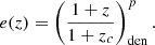
where e(z) characterises the redshift evolution of the local luminosity function and is expressed as
 (A.3)
(A.3)
Given our definition for the XLAF (see Eq. 2, Sect. 3.3), we need to assume a functional form for the absorption function, fabs. Following the methodology of Ueda et al. (2003), we modelled the absorption function using piecewise constant functions across discrete NH bins. Given the redshift range of our study and the energy coverage of XMM-Newton and Chandra, X-ray absorption cannot be reliably constraint for column densities below ∼1023 cm−2. We therefore defined the absorption function in three NH intervals as follows:
![Mathematical equation: $$ \begin{aligned} f_{\rm abs}(N_{\rm H}, z, L_{\rm X}) = {\left\{ \begin{array}{ll} \dfrac{1}{3} - \dfrac{\varepsilon }{3(1 + \varepsilon )} \psi (z,L_{\rm X})&[20 \le \log N_{\rm H} < 23] \\ \dfrac{\varepsilon }{1 + \varepsilon } \psi (z, L_{\rm X})&[23 \le \log N_{\rm H} < 24] \\ \dfrac{f_{\mathrm{CTK} ,r}}{2}\,\psi (z, L_{\rm X})&[24 \le \log N_{\rm H} < 26] \end{array}\right.} \end{aligned} $$](/articles/aa/full_html/2026/08/aa58018-25/aa58018-25-eq45.gif) (A.4)
(A.4)
In this parametrisation, ε represents the ratio between the number of sources with 23 ≤ log NH < 24 and those with 22 ≤ log NH < 23, while fCTK, r denotes the relative fraction of CTK sources with respect to absorbed Compton-thin AGNs (Vijarnwannaluk et al. 2022).
The quantity ψ(z, LX) corresponds to the fraction of absorbed Compton-thin AGNs relative to the total AGN population. It incorporates both the redshift and luminosity dependence and is parametrised as a linear function of log LX:
 (A.5)
(A.5)
where we adopt ψmin = 0.2 and ψmax = 0.99. The parameter C controls the luminosity dependence, while ψ43.75(z) represents the absorption fraction for AGNs with log LX = 43.75 at a given redshift.
For z < 2, ψ43.75(z) is well constrained (Ueda et al. 2014), whereas above this redshift it is typically assumed constant (e.g. 2 ≤ z < 3; Vijarnwannaluk et al. 2022). In this work, we extended the definition of ψ43.75(z) for z ≥ 3 as:
 (A.6)
(A.6)
where ψ3 denotes the absorption fraction at log LX = 43.75 and z = 3, and a2 is the redshift evolution index.
A.2. Bayesian inference framework
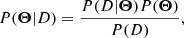
We employed a Bayesian approach to estimate simultaneously the parametric form of the XLF and the absorption function. Given a dataset of n observations, D = {di; i = 1, …, n}, and a model for the XLF described by a set of parameters Θ, Bayes’ theorem gives:
 (A.7)
(A.7)
where P(Θ|D) is the posterior probability of the model given the data, ℒ = P(D|Θ) is the likelihood of obtaining the data for a given model, P(Θ) is the prior probability of the model parameters, and P(D) = ∫P(Θ|D)dΘ is the evidence.
To sample the posterior distribution of the model parameters, we used the nested-sampling Monte Carlo algorithm MLFriends (Buchner 2016; Buchner & Bauer 2017), implemented in the UltraNest package. Nested sampling enables simultaneous exploration of the posterior distribution and computation of the Bayesian evidence, which allows a direct comparison between alternative XLF models through Bayes factors. This approach also provides a rigorous treatment of the uncertainties in the X-ray spectral parameters and photometric redshifts of the individual sources included in the analysis.
We adopted flat (uniform or log-uniform) priors for all free parameters, spanning ranges broad enough to encompass the values reported in previous studies. Table A.1 lists the adopted prior limits for each parameter of the XLAF model.
Prior limits and best-fitting values for the free parameters of the X-ray luminosity and absorption functions.
Following the formulation of Loredo (2004), the likelihood of observing a given dataset can be expressed as the product of the probabilities of detecting each individual source multiplied by the probability of not detecting any additional sources. The corresponding log-likelihood, following Buchner et al. 2015, is:
 (A.8)
(A.8)
where λ represents the expected number of detected sources in a Poisson process for an XLF model with parameters Θ:
 (A.9)
(A.9)
and ϕabs = ϕ × fabs, where ϕ and fabs are the luminosity and absorption functions defined above. Ω(LX, z, NH) is the survey sensitivity function, for which we adopted the values calculated by Pouliasis et al. (2024).
The term Pi in Eq. A.8 is defined as:
 (A.10)
where p(di|LX, z, NH) is the probability that source i has X-ray properties (LX, z, NH), given by the posterior distributions obtained from the Bayesian X-ray spectral fitting. Alternatively, the IR-updated posteriors discussed in Sect. 3.2 can be used here. The inclusion of Ω within this term accounts for the loss of information caused by differences between X-ray source detection and spectral fitting procedures (see Buchner et al. 2015, Appendix A, for a detailed discussion).
The integral in Eq. A.8 is evaluated using importance-sampling integration techniques (Kloek & van Dijk 1978; Press et al. 2007). The integration limits adopted for z, log LX, and log NH are [3, 6], [42, 47], and [20, 26], respectively.
Our combined parametrisation of the luminosity and absorption functions includes ten free parameters. Table A.1 lists the best-fitting parameter values and their uncertainties for the assumed PDE model. Figure A.2 shows the one-dimensional (diagonal panels) and two-dimensional marginal posterior distributions of the XLAF parameters. Results based on X-ray–only posteriors are shown in grey, while those incorporating IR-updated posteriors are shown in red. Most luminosity-function parameters remain consistent within 2σ between the two cases, whereas the inclusion of IR data shifts the absorption-related parameters ε and fCTK, r toward lower values. The parameters governing the redshift evolution of the absorption function (ψ3, C, and a2) remain poorly constrained, indicating that our dataset does not provide significant evidence for absorption-function evolution within the studied redshift range.
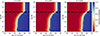 |
Fig. A.1. Sensitivity maps (Ω) for our survey. Each panel show the detection probability in the log LX, log NH plane at three redshift values (3.0, 4.0, 6.0). |
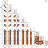 |
Fig. A.2. 1D and 2D marginal posterior distributions for the XLAF parameters. Black: X-ray only posteriors; red: posteriors updated with IR data. |
Appendix B: X-ray properties
This appendix presents, in Figs. B.1 and B.2, the X-ray cutouts and spectra for the ten CTK AGN candidates included in our sample. For each source, we show the Chandra or XMM-Newton images in the observed 0.5−2 and 2−7 keV bands, together with the corresponding X-ray spectrum and best-fitting model derived from the Bayesian spectral analysis. We also display the marginalised posterior distributions for three key parameters: NH, LX and z. For sources with spectroscopic redshifts, the z distribution is represented by a single vertical red line.
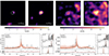 |
Fig. B.1. XMM-Newton cutouts and spectra for the selected CTK candidates. Top: Two arc-minutes XMM-Newton-EPIC cutouts in the 0.5-2 keV (left) and 2-7 keV (right) bands. Bottom: Co-added, background-subtracted XMM-Newton-EPIC spectrum. To improve visualization, the spectrum is binned. The red-shaded areas show the one- and two-sigma uncertainties for the best-fit source model (red, solid line). On the right column we plot the posterior distribution for log NH (top), log LX (middle), and redshift (bottom). The red, dashed lines show the mode of each distribution. |
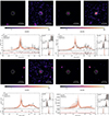 |
Fig. B.2. Chandra cutouts and spectra for the selected CTK candidates. Top: One arc-minutes Chandra-ACIS cutouts in the 0.5-2 keV (left) and 2-7 keV (right) bands. Bottom: Co-added, background-subtracted Chandra-ACIS spectrum. To improve visualization, the spectrum is binned. The red-shaded areas show the one- and two-sigma uncertainties for the best-fit source model (red, solid line). On the right column we plot the posterior distribution for log NH (top), log LX (middle), and redshift (bottom). The red, dashed lines show the mode of each distribution. |
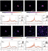 |
Fig. B.2. Continued. |
These figures illustrate the data quality and spectral characteristics of the selected CTK candidates, highlighting the range of absorption levels and luminosities found within the sample. They also provide a visual summary of the Bayesian modelling results, allowing a direct assessment of the uncertainties and degeneracies that affect the determination of NH and LX for individual sources.
CIGALE modules and parameter grid.
Appendix C: Grid of models for CIGALE
In this appendix we present the modules and parameter values (see Table B.1) we used in CIGALE for the modelling of the SED of CTK objects.
All Tables
Prior limits and best-fitting values for the free parameters of the X-ray luminosity and absorption functions.
All Figures
|
Fig. 1. Intrinsic X-ray luminosity in the 2−10 keV band versus hydrogen column density. Small circles show the full sample from Pouliasis et al. (2024), shaded by the probability of being CTK. Large circles mark our selection of CTK candidates, as described in Sect. 2.1, colour-coded according to their parent X-ray survey: CDF (yellow), CCLS (red), XXL-N (blue). For clarity, error bars (indicating 90% credible intervals) are shown only for the CTK candidates. |
| In the text | |
|
Fig. 2. SED of source lid_1278 (z = 3.013), one of the CTK AGN candidates in our sample. The colour-coded symbols show the observed photometry from CFHT-MegaCam (purple), Subaru-HSC (blue), VISTA (green), Spitzer/IRAC (orange), and Spitzer/MIPS (red). The solid black line indicates the best-fitting total model from CIGALE, decomposed into the AGN (disc + torus; dashed red line) and host-galaxy (stars + dust; dotted grey line) components. The predicted 6 μm flux derived from the X-ray luminosity is also shown (red cross). The best-fitting parameters are reported in the legend, including inclination angle and AGN fractional contribution. |
| In the text | |
|
Fig. 3. Intrinsic X-ray luminosity in the 2−10 keV band versus the monochromatic 6 μm luminosity of the AGN component. The results for our CTK sample are shown before (left panel) and after (right panel) applying the IR luminosity prior, as described in Sect. 3.2. Grey dots represent the X-ray–selected AGN sample from Laloux et al. (2023) in the CCLS field. Large circles indicate our final CTK candidates, colour-coded by their parent X-ray survey: CDF (yellow), CCLS (red), XXL-N (blue). The dashed black line marks the LX − L6 μm relation from Stern (2015), while the dashed grey lines denote the 2σ dispersion of the Laloux et al. (2023) sample with respect to that relation. |
| In the text | |
|
Fig. 4. Joint posterior distribution in the log NH − log L6 μm plane (shaded blue region) for source lid_1278, one of our CTK candidates. The IR luminosity L6 μm is inferred from the X-ray luminosity posterior via the Stern (2015) relation. The dashed black line and the shaded grey region show the SED-inferred L6 μm value and its uncertainty, while the red dotted contours indicate the posterior distribution after incorporating the IR prior. |
| In the text | |
|
Fig. 5. Observed distributions of hydrogen column density and X-ray luminosity for the full Pouliasis et al. (2024) sample. The black-hatched histograms show the original X-ray posteriors, while the solid red histograms correspond to the posteriors updated with IR information (see Sect. 3.2). |
| In the text | |
|
Fig. 6. Probability that the selected CTK candidates have log NH > 24. Grey bars show the original probabilities estimated using the X-ray only posteriors, and red bars show the results using the IR-updated posteriors. Light grey areas show the estimated probabilities before applying the redshift corrections discussed in Sect. 2.1. The vertical dashed black line shows our initial selection criterion for the CTK sample. |
| In the text | |
|
Fig. 7. XLAF for two redshift intervals (z = 3 − 4, top panels; z = 4 − 6, bottom panels) and two hydrogen column density ranges (log NH = 20 − 24, left panels; log NH = 24 − 26, right panels). Black lines and grey shaded regions indicate the results for the parametric XLAF obtained from the X-ray-only posteriors, while red lines and shaded regions correspond to those derived using the IR luminosity priors. The corresponding binned XLAFs were derived using the Miyaji et al. (2001) method. |
| In the text | |
|
Fig. 8. XLF for the CTK population (24 < log NH < 26). Red symbols show our result for the parametric XLF in the 3−6 redshift range. The solid red line corresponds to the median value and shaded areas are the 1σ (darker red) and 2σ (lighter red) uncertainties. The dashed black line is the XLF for CTK sources in the local universe (z < 0.05) derived by Georgantopoulos et al. (2025). The grey-hatched area is the non-parametric XLF in the 3.1−7 redshift range estimated by Buchner et al. (2015). The area shows the 90% confidence region. The dotted blue line corresponds to the Aird et al. (2015b) XLF for CTK AGNs in the 3−6 redshift range. |
| In the text | |
|
Fig. 9. Evolution of the fraction of CTK sources over the total AGN population across redshift. Our results are shown with the red shaded regions, which represent the 1σ (darker red) and 2σ (lighter red) confidence regions. The grey-hatched area corresponds to the Buchner et al. (2015) results (90% confidence interval) for AGNs in the 43.2 ≤ log LX ≤ 43.6 interval. The blue-hatched area shows the Aird et al. (2015b) estimates (99% confidence interval) for sources with log LX = 43.5. The green squares show the Laloux et al. (2023) results; quoted upper limits are 3σ. Pink triangles correspond to the results by Lanzuisi et al. (2018) and purple diamond corresponds to a study by Masini et al. (2018). The black (Georgantopoulos et al. 2025) and yellow (Burlon et al. 2011) circles show the CTK fraction in the local Universe using Swift/BAT selected AGNs. Red diamonds show the fraction of CTK sources estimated through the integration of the Ananna et al. (2019) luminosity function. Open symbols show the result in the range (24 ≤ log NH < 26), while filled symbols are for (24 ≤ log NH < 25). |
| In the text | |
|
Fig. A.1. Sensitivity maps (Ω) for our survey. Each panel show the detection probability in the log LX, log NH plane at three redshift values (3.0, 4.0, 6.0). |
| In the text | |
|
Fig. A.2. 1D and 2D marginal posterior distributions for the XLAF parameters. Black: X-ray only posteriors; red: posteriors updated with IR data. |
| In the text | |
|
Fig. B.1. XMM-Newton cutouts and spectra for the selected CTK candidates. Top: Two arc-minutes XMM-Newton-EPIC cutouts in the 0.5-2 keV (left) and 2-7 keV (right) bands. Bottom: Co-added, background-subtracted XMM-Newton-EPIC spectrum. To improve visualization, the spectrum is binned. The red-shaded areas show the one- and two-sigma uncertainties for the best-fit source model (red, solid line). On the right column we plot the posterior distribution for log NH (top), log LX (middle), and redshift (bottom). The red, dashed lines show the mode of each distribution. |
| In the text | |
|
Fig. B.2. Chandra cutouts and spectra for the selected CTK candidates. Top: One arc-minutes Chandra-ACIS cutouts in the 0.5-2 keV (left) and 2-7 keV (right) bands. Bottom: Co-added, background-subtracted Chandra-ACIS spectrum. To improve visualization, the spectrum is binned. The red-shaded areas show the one- and two-sigma uncertainties for the best-fit source model (red, solid line). On the right column we plot the posterior distribution for log NH (top), log LX (middle), and redshift (bottom). The red, dashed lines show the mode of each distribution. |
| In the text | |
|
Fig. B.2. Continued. |
| In the text | |
Current usage metrics show cumulative count of Article Views (full-text article views including HTML views, PDF and ePub downloads, according to the available data) and Abstracts Views on Vision4Press platform.
Data correspond to usage on the plateform after 2015. The current usage metrics is available 48-96 hours after online publication and is updated daily on week days.
Initial download of the metrics may take a while.