


| Issue |
A&A
Volume 711, July 2026
Euclid Quick Data Release (Q1)
|
|
|---|---|---|
| Article Number | A20 | |
| Number of page(s) | 30 | |
| Section | Catalogs and data | |
| DOI | https://doi.org/10.1051/0004-6361/202554619 | |
| Published online | 30 June 2026 | |
Euclid Quick Data Release (Q1)
XX. The active galaxies of Euclid
1
School of Physics, HH Wills Physics Laboratory, University of Bristol, Tyndall Avenue, Bristol BS8 1TL, UK
2
Department of Mathematics and Physics, Roma Tre University, Via della Vasca Navale 84, 00146 Rome, Italy
3
INAF-Osservatorio Astronomico di Roma, Via Frascati 33, 00078 Monteporzio Catone, Italy
4
INAF-Osservatorio di Astrofisica e Scienza dello Spazio di Bologna, Via Piero Gobetti 93/3, 40129 Bologna, Italy
5
Department of Physics and Helsinki Institute of Physics, Gustaf Hällströmin katu 2, 00014 University of Helsinki, Finland
6
Institute of Space Sciences (ICE, CSIC), Campus UAB, Carrer de Can Magrans, s/n, 08193 Barcelona, Spain
7
Institut d’Estudis Espacials de Catalunya (IEEC), Edifici RDIT, Campus UPC, 08860 Castelldefels, Barcelona, Spain
8
INAF-Osservatorio Astronomico di Capodimonte, Via Moiariello 16, 80131 Napoli, Italy
9
Max Planck Institute for Extraterrestrial Physics, Giessenbachstr. 1, 85748 Garching, Germany
10
Max-Planck-Institut für Astronomie, Königstuhl 17, 69117 Heidelberg, Germany
11
INAF-Osservatorio Astronomico di Padova, Via dell’Osservatorio 5, 35122 Padova, Italy
12
Leiden Observatory, Leiden University, Einsteinweg 55, 2333 CC Leiden, The Netherlands
13
Kapteyn Astronomical Institute, University of Groningen, PO Box 800, 9700 AV Groningen, The Netherlands
14
SRON Netherlands Institute for Space Research, Landleven 12, 9747 AD, Groningen, The Netherlands
15
Department of Astronomy, University of Geneva, ch. d’Ecogia 16, 1290 Versoix, Switzerland
16
INAF-Osservatorio Astrofisico di Arcetri, Largo E. Fermi 5, 50125 Firenze, Italy
17
Dipartimento di Fisica e Astronomia “Augusto Righi” – Alma Mater Studiorum Università di Bologna, Via Piero Gobetti 93/2, 40129 Bologna, Italy
18
Dipartimento di Fisica e Astronomia, Università di Firenze, Via G. Sansone 1, 50019 Sesto Fiorentino, Firenze, Italy
19
University of Trento, Via Sommarive 14, I-38123 Trento, Italy
20
Instituto de Astrofísica de Canarias (IAC); Departamento de Astrofísica, Universidad de La Laguna (ULL), 38200 La Laguna, Tenerife, Spain
21
Universitäts-Sternwarte München, Fakultät für Physik, Ludwig-Maximilians-Universität München, Scheinerstrasse 1, 81679 München, Germany
22
INAF, Istituto di Radioastronomia, Via Piero Gobetti 101, 40129 Bologna, Italy
23
Department of Physics, Centre for Extragalactic Astronomy, Durham University, South Road, Durham DH1 3LE, UK
24
STAR Institute, University of Liège, Quartier Agora, Allée du six Août 19c, 4000 Liège, Belgium
25
School of Physics & Astronomy, University of Southampton, Highfield Campus, Southampton SO17 1BJ, UK
26
INAF-Istituto di Astrofisica e Planetologia Spaziali, Via del Fosso del Cavaliere, 100, 00100 Roma, Italy
27
Department of Physics and Astronomy, University of British Columbia, Vancouver, BC V6T 1Z1, Canada
28
Department of Physical Sciences, Ritsumeikan University, Kusatsu, Shiga 525-8577, Japan
29
National Astronomical Observatory of Japan, 2-21-1 Osawa, Mitaka, Tokyo 181-8588, Japan
30
Academia Sinica Institute of Astronomy and Astrophysics (ASIAA), 11F of ASMAB, No. 1, Section 4, Roosevelt Road, Taipei 10617, Taiwan
31
Université Paris-Saclay, CNRS, Institut d’astrophysique spatiale, 91405 Orsay, France
32
ESAC/ESA, Camino Bajo del Castillo, s/n., Urb. Villafranca del Castillo, 28692 Villanueva de la Cañada, Madrid, Spain
33
School of Mathematics and Physics, University of Surrey, Guildford, Surrey, GU2 7XH, UK
34
INAF-Osservatorio Astronomico di Brera, Via Brera 28, 20122 Milano, Italy
35
Université Paris-Saclay, Université Paris Cité, CEA, CNRS, AIM, 91191 Gif-sur-Yvette, France
36
IFPU, Institute for Fundamental Physics of the Universe, Via Beirut 2, 34151 Trieste, Italy
37
INAF-Osservatorio Astronomico di Trieste, Via G. B. Tiepolo 11, 34143 Trieste, Italy
38
INFN, Sezione di Trieste, Via Valerio 2, 34127 Trieste TS, Italy
39
SISSA, International School for Advanced Studies, Via Bonomea 265, 34136 Trieste TS, Italy
40
Dipartimento di Fisica e Astronomia, Università di Bologna, Via Gobetti 93/2, 40129 Bologna, Italy
41
INFN-Sezione di Bologna, Viale Berti Pichat 6/2, 40127 Bologna, Italy
42
Centre National d’Etudes Spatiales – Centre spatial de Toulouse, 18 avenue Edouard Belin, 31401 Toulouse Cedex 9, France
43
Space Science Data Center, Italian Space Agency, Via del Politecnico snc, 00133 Roma, Italy
44
Dipartimento di Fisica, Università di Genova, Via Dodecaneso 33, 16146 Genova, Italy
45
INFN-Sezione di Genova, Via Dodecaneso 33, 16146 Genova, Italy
46
Department of Physics “E. Pancini”, University Federico II, Via Cinthia 6, 80126 Napoli, Italy
47
Instituto de Astrofísica e Ciências do Espaço, Universidade do Porto, CAUP, Rua das Estrelas, PT4150-762 Porto, Portugal
48
Faculdade de Ciências da Universidade do Porto, Rua do Campo de Alegre, 4150-007 Porto, Portugal
49
Dipartimento di Fisica, Università degli Studi di Torino, Via P. Giuria 1, 10125 Torino, Italy
50
INFN-Sezione di Torino, Via P. Giuria 1, 10125 Torino, Italy
51
INAF-Osservatorio Astrofisico di Torino, Via Osservatorio 20, 10025 Pino Torinese (TO), Italy
52
European Space Agency/ESTEC, Keplerlaan 1, 2201 AZ Noordwijk, The Netherlands
53
Institute Lorentz, Leiden University, Niels Bohrweg 2, 2333 CA Leiden, The Netherlands
54
INAF-IASF Milano, Via Alfonso Corti 12, 20133 Milano, Italy
55
Centro de Investigaciones Energéticas, Medioambientales y Tecnológicas (CIEMAT), Avenida Complutense 40, 28040 Madrid, Spain
56
Port d’Informació Científica, Campus UAB, C. Albareda s/n, 08193 Bellaterra (Barcelona), Spain
57
Institute for Theoretical Particle Physics and Cosmology (TTK), RWTH Aachen University, 52056 Aachen, Germany
58
INFN section of Naples, Via Cinthia 6, 80126 Napoli, Italy
59
Institute for Astronomy, University of Hawaii, 2680 Woodlawn Drive, Honolulu, HI 96822, USA
60
Dipartimento di Fisica e Astronomia “Augusto Righi” – Alma Mater Studiorum Università di Bologna, Viale Berti Pichat 6/2, 40127 Bologna, Italy
61
Instituto de Astrofísica de Canarias, Vía Láctea, 38205 La Laguna, Tenerife, Spain
62
Institute for Astronomy, University of Edinburgh, Royal Observatory, Blackford Hill, Edinburgh EH9 3HJ, UK
63
Jodrell Bank Centre for Astrophysics, Department of Physics and Astronomy, University of Manchester, Oxford Road, Manchester M13 9PL, UK
64
European Space Agency/ESRIN, Largo Galileo Galilei 1, 00044 Frascati, Roma, Italy
65
Université Claude Bernard Lyon 1, CNRS/IN2P3, IP2I Lyon, UMR 5822, Villeurbanne F-69100, France
66
Institut de Ciències del Cosmos (ICCUB), Universitat de Barcelona (IEEC-UB), Martí i Franquès 1, 08028 Barcelona, Spain
67
Institució Catalana de Recerca i Estudis Avançats (ICREA), Passeig de Lluís Companys 23, 08010 Barcelona, Spain
68
UCB Lyon 1, CNRS/IN2P3, IUF, IP2I Lyon, 4 rue Enrico Fermi, 69622 Villeurbanne, France
69
Mullard Space Science Laboratory, University College London, Holmbury St Mary, Dorking, Surrey, RH5 6NT, UK
70
Departamento de Física, Faculdade de Ciências, Universidade de Lisboa, Edifício C8, Campo Grande, PT1749-016 Lisboa, Portugal
71
Instituto de Astrofísica e Ciências do Espaço, Faculdade de Ciências, Universidade de Lisboa, Campo Grande, 1749-016 Lisboa, Portugal
72
INFN-Padova, Via Marzolo 8, 35131 Padova, Italy
73
Aix-Marseille Université, CNRS/IN2P3, CPPM, Marseille, France
74
INFN-Bologna, Via Irnerio 46, 40126 Bologna, Italy
75
FRACTAL S.L.N.E., calle Tulipán 2, Portal 13 1A, 28231 Las Rozas de Madrid, Spain
76
NRC Herzberg, 5071 West Saanich Rd, Victoria, BC V9E 2E7, Canada
77
Institute of Theoretical Astrophysics, University of Oslo, P.O. Box 1029 Blindern, 0315 Oslo, Norway
78
Jet Propulsion Laboratory, California Institute of Technology, 4800 Oak Grove Drive, Pasadena, CA, 91109, USA
79
Department of Physics, Lancaster University, Lancaster LA1 4YB, UK
80
Felix Hormuth Engineering, Goethestr. 17, 69181 Leimen, Germany
81
Technical University of Denmark, Elektrovej 327, 2800 Kgs. Lyngby, Denmark
82
Cosmic Dawn Center (DAWN), DTU Space, Elektrovej 327., 2800 Kgs. Lyngby, Denmark
83
Institut d’Astrophysique de Paris, UMR 7095, CNRS, and Sorbonne Université, 98 bis boulevard Arago, 75014 Paris, France
84
NASA Goddard Space Flight Center, Greenbelt, MD 20771, USA
85
Université de Genève, Département de Physique Théorique and Centre for Astroparticle Physics, 24 quai Ernest-Ansermet, CH-1211 Genève 4, Switzerland
86
Department of Physics, P.O. Box 64, 00014 University of Helsinki, Finland
87
Helsinki Institute of Physics, Gustaf Hållströmin katu 2, University of Helsinki, Helsinki, Finland
88
Centre de Calcul de l’IN2P3/CNRS, 21 avenue Pierre de Coubertin 69627 Villeurbanne Cedex, France
89
Laboratoire d’etude de l’Univers et des phenomenes eXtremes, Observatoire de Paris, Université PSL, Sorbonne Université, CNRS, 92190 Meudon, France
90
Aix-Marseille Université, CNRS, CNES, LAM, Marseille, France
91
SKA Observatory, Jodrell Bank, Lower Withington, Macclesfield, Cheshire, SK11 9FT, UK
92
Dipartimento di Fisica “Aldo Pontremoli”, Università degli Studi di Milano, Via Celoria 16, 20133 Milano, Italy
93
INFN-Sezione di Milano, Via Celoria 16, 20133 Milano, Italy
94
University of Applied Sciences and Arts of Northwestern Switzerland, School of Computer Science, 5210 Windisch, Switzerland
95
Universität Bonn, Argelander-Institut für Astronomie, Auf dem Hügel 71, 53121 Bonn, Germany
96
INFN-Sezione di Roma, Piazzale Aldo Moro, 2 – c/o Dipartimento di Fisica, Edificio G. Marconi, 00185 Roma, Italy
97
Department of Physics, Institute for Computational Cosmology, Durham University, South Road, Durham DH1 3LE, UK
98
Infrared Processing and Analysis Center, California Institute of Technology, Pasadena, CA 91125, USA
99
Université Côte d’Azur, Observatoire de la Côte d’Azur, CNRS, Laboratoire Lagrange, Bd de l’Observatoire, CS 34229, 06304 Nice cedex 4, France
100
Université Paris Cité, CNRS, Astroparticule et Cosmologie, 75013 Paris, France
101
CNRS-UCB International Research Laboratory, Centre Pierre Binetruy, IRL2007, CPB-IN2P3, Berkeley, USA
102
University of Applied Sciences and Arts of Northwestern Switzerland, School of Engineering, 5210 Windisch, Switzerland
103
Institut d’Astrophysique de Paris, 98bis Boulevard Arago, 75014 Paris, France
104
Institute of Physics, Laboratory of Astrophysics, Ecole Polytechnique Fédérale de Lausanne (EPFL), Observatoire de Sauverny, 1290 Versoix, Switzerland
105
Aurora Technology for European Space Agency (ESA), Camino bajo del Castillo, s/n, Urbanizacion Villafranca del Castillo, Villanueva de la Cañada, 28692 Madrid, Spain
106
Institut de Física d’Altes Energies (IFAE), The Barcelona Institute of Science and Technology, Campus UAB, 08193 Bellaterra (Barcelona), Spain
107
School of Mathematics, Statistics and Physics, Newcastle University, Herschel Building, Newcastle-upon-Tyne, NE1 7RU, UK
108
DARK, Niels Bohr Institute, University of Copenhagen, Jagtvej 155, 2200 Copenhagen, Denmark
109
Waterloo Centre for Astrophysics, University of Waterloo, Waterloo, Ontario N2L 3G1, Canada
110
Department of Physics and Astronomy, University of Waterloo, Waterloo, Ontario N2L 3G1, Canada
111
Perimeter Institute for Theoretical Physics, Waterloo, Ontario N2L 2Y5, Canada
112
Institute of Space Science, Str. Atomistilor, nr. 409Măgurele, Ilfov 077125, Romania
113
Consejo Superior de Investigaciones Cientificas, Calle Serrano 117, 28006 Madrid, Spain
114
Universidad de La Laguna, Departamento de Astrofísica, 38206 La Laguna, Tenerife, Spain
115
Dipartimento di Fisica e Astronomia “G. Galilei”, Università di Padova, Via Marzolo 8, 35131 Padova, Italy
116
Caltech/IPAC, 1200 E. California Blvd., Pasadena, CA 91125, USA
117
Institut für Theoretische Physik, University of Heidelberg, Philosophenweg 16, 69120 Heidelberg, Germany
118
Institut de Recherche en Astrophysique et Planétologie (IRAP), Université de Toulouse, CNRS, UPS, CNES, 14 Av. Edouard Belin, 31400 Toulouse, France
119
Université St Joseph; Faculty of Sciences, Beirut, Lebanon
120
Departamento de Física, FCFM, Universidad de Chile, Blanco Encalada 2008, Santiago, Chile
121
Universität Innsbruck, Institut für Astro- und Teilchenphysik, Technikerstr. 25/8, 6020 Innsbruck, Austria
122
Satlantis, University Science Park, Sede Bld 48940, Leioa-Bilbao, Spain
123
Centre for Electronic Imaging, Open University, Walton Hall, Milton Keynes, MK7 6AA, UK
124
Instituto de Astrofísica e Ciências do Espaço, Faculdade de Ciências, Universidade de Lisboa, Tapada da Ajuda, 1349-018 Lisboa, Portugal
125
Cosmic Dawn Center (DAWN), DTU Space, Elektrovej 327., 2800 Kgs. Lyngby, Denmark
126
Niels Bohr Institute, University of Copenhagen, Jagtvej 128, 2200 Copenhagen, Denmark
127
Universidad Politécnica de Cartagena, Departamento de Electrónica y Tecnología de Computadoras, Plaza del Hospital 1, 30202 Cartagena, Spain
128
Dipartimento di Fisica e Scienze della Terra, Università degli Studi di Ferrara, Via Giuseppe Saragat 1, 44122 Ferrara, Italy
129
Istituto Nazionale di Fisica Nucleare, Sezione di Ferrara, Via Giuseppe Saragat 1, 44122 Ferrara, Italy
130
School of Physics and Astronomy, Cardiff University, The Parade, Cardiff CF24 3AA, UK
131
Department of Physics, Oxford University, Keble Road, Oxford OX1 3RH, UK
132
INAF – Osservatorio Astronomico di Brera, Via Emilio Bianchi 46, 23807 Merate, Italy
133
INAF-Osservatorio Astronomico di Brera, Via Brera 28, 20122 Milano, Italy, and INFN-Sezione di Genova, Via Dodecaneso 33, 16146, Genova, Italy
134
ICL, Junia, Université Catholique de Lille, LITL, 59000 Lille, France
135
ICSC – Centro Nazionale di Ricerca in High Performance Computing, Big Data e Quantum Computing, Via Magnanelli 2, Bologna, Italy
136
Instituto de Física Teórica UAM-CSIC, Campus de Cantoblanco, 28049 Madrid, Spain
137
CERCA/ISO, Department of Physics, Case Western Reserve University, 10900 Euclid Avenue, Cleveland, OH 44106, USA
138
Technical University of Munich, TUM School of Natural Sciences, Physics Department, James-Franck-Str. 1, 85748 Garching, Germany
139
Max-Planck-Institut für Astrophysik, Karl-Schwarzschild-Str. 1, 85748 Garching, Germany
140
Laboratoire Univers et Théorie, Observatoire de Paris, Université PSL, Université Paris Cité, CNRS, 92190 Meudon, France
141
Departamento de Física Fundamental, Universidad de Salamanca, Plaza de la Merced s/n, 37008 Salamanca, Spain
142
Université de Strasbourg, CNRS, Observatoire astronomique de Strasbourg, UMR 7550, 67000 Strasbourg, France
143
Center for Data-Driven Discovery, Kavli IPMU (WPI), UTIAS, The University of Tokyo, Kashiwa, Chiba 277-8583, Japan
144
Ludwig-Maximilians-University, Schellingstrasse 4, 80799 Munich, Germany
145
Max-Planck-Institut für Physik, Boltzmannstr. 8, 85748 Garching, Germany
146
California Institute of Technology, 1200 E California Blvd, Pasadena, CA 91125, USA
147
Department of Physics & Astronomy, University of California Irvine, Irvine, CA 92697, USA
148
Department of Mathematics and Physics E. De Giorgi, University of Salento, Via per Arnesano, CP-I93, 73100 Lecce, Italy
149
INFN, Sezione di Lecce, Via per Arnesano, CP-193, 73100 Lecce, Italy
150
INAF-Sezione di Lecce, c/o Dipartimento Matematica e Fisica, Via per Arnesano, 73100 Lecce, Italy
151
Departamento Física Aplicada, Universidad Politécnica de Cartagena, Campus Muralla del Mar, 30202 Cartagena, Murcia, Spain
152
Instituto de Física de Cantabria, Edificio Juan Jordá, Avenida de los Castros, 39005 Santander, Spain
153
CEA Saclay, DFR/IRFU, Service d’Astrophysique, Bat. 709, 91191 Gif-sur-Yvette, France
154
Institute of Cosmology and Gravitation, University of Portsmouth, Portsmouth PO1 3FX, UK
155
Department of Computer Science, Aalto University, PO Box 15400 Espoo FI-00 076, Finland
156
Dipartimento di Fisica – Sezione di Astronomia, Università di Trieste, Via Tiepolo 11, 34131 Trieste, Italy
157
Instituto de Astrofísica de Canarias, c/ Via Lactea s/n, La Laguna 38200, Spain. Departamento de Astrofísica de la Universidad de La Laguna, Avda. Francisco Sanchez, La Laguna, 38200, Spain
158
Ruhr University Bochum, Faculty of Physics and Astronomy, Astronomical Institute (AIRUB), German Centre for Cosmological Lensing (GCCL), 44780 Bochum, Germany
159
Department of Physics and Astronomy, Vesilinnantie 5, 20014 University of Turku, Finland
160
Serco for European Space Agency (ESA), Camino bajo del Castillo, s/n, Urbanizacion Villafranca del Castillo, Villanueva de la Cañada, 28692 Madrid, Spain
161
ARC Centre of Excellence for Dark Matter Particle Physics, Melbourne, Australia
162
Centre for Astrophysics & Supercomputing, Swinburne University of Technology, Hawthorn, Victoria 3122, Australia
163
Department of Physics and Astronomy, University of the Western Cape, Bellville, Cape Town, 7535, South Africa
164
DAMTP, Centre for Mathematical Sciences, Wilberforce Road, Cambridge CB3 0WA, UK
165
Kavli Institute for Cosmology Cambridge, Madingley Road, Cambridge CB3 0HA, UK
166
Department of Astrophysics, University of Zurich, Winterthurerstrasse 190, 8057 Zurich, Switzerland
167
IRFU, CEA, Université Paris-Saclay, 91191 Gif-sur-Yvette Cedex, France
168
Oskar Klein Centre for Cosmoparticle Physics, Department of Physics, Stockholm University, Stockholm SE-106 91, Sweden
169
Astrophysics Group, Blackett Laboratory, Imperial College London, London SW7 2AZ, UK
170
Univ. Grenoble Alpes, CNRS, Grenoble INP, LPSC-IN2P3, 53, Avenue des Martyrs, 38000 Grenoble, France
171
Dipartimento di Fisica, Sapienza Università di Roma, Piazzale Aldo Moro 2, 00185 Roma, Italy
172
Centro de Astrofísica da Universidade do Porto, Rua das Estrelas, 4150-762 Porto, Portugal
173
HE Space for European Space Agency (ESA), Camino bajo del Castillo, s/n, Urbanizacion Villafranca del Castillo, Villanueva de la Cañada, 28692 Madrid, Spain
174
Department of Astrophysical Sciences, Peyton Hall, Princeton University, Princeton, NJ 08544, USA
175
Theoretical astrophysics, Department of Physics and Astronomy, Uppsala University, Box 515, 751 20 Uppsala, Sweden
176
Mathematical Institute, University of Leiden, Einsteinweg 55, 2333 CA Leiden, The Netherlands
177
ASTRON, the Netherlands Institute for Radio Astronomy, Postbus 2, 7990 AA, Dwingeloo, The Netherlands
178
Anton Pannekoek Institute for Astronomy, University of Amsterdam, Postbus 94249, 1090 GE Amsterdam, The Netherlands
179
Center for Advanced Interdisciplinary Research, Ss. Cyril and Methodius University in Skopje, Macedonia
180
Institute of Astronomy, University of Cambridge, Madingley Road, Cambridge CB3 0HA, UK
181
Department of Physics and Astronomy, University of California, Davis, CA 95616, USA
182
Space physics and astronomy research unit, University of Oulu, Pentti Kaiteran katu 1, FI-90014 Oulu, Finland
183
Center for Computational Astrophysics, Flatiron Institute, 162 5th Avenue, 10010 New York, NY, USA
★ Corresponding author: This email address is being protected from spambots. You need JavaScript enabled to view it.
Received:
18
March
2025
Accepted:
16
June
2025
Abstract
We present three catalogues of candidate active galactic nuclei (AGN) in the Euclid Quick Release (Q1) fields. For each Euclid source, we collected multi-wavelength photometric and spectroscopic information from surveys such as the Galaxy Evolution Explorer (GALEX), Gaia, the Dark Energy Survey (DES), the Wide-field Infrared Survey Explorer (WISE), Spitzer, the Dark Energy Spectroscopic Instrument (DESI), and the Sloan Digital Sky Survey (SDSS), including spectroscopic redshifts from public compilations when available. We investigated the AGN content of the Q1 fields using multiple selection methods. Applying Euclid colours and WISE-AllWISE cuts, we identified 292 222 and 65 131 candidates, respectively. We compiled a high-purity QSO catalogue based on Gaia DR3 information, containing 1971 candidates. Using spectroscopic information from DESI, we performed broad-line and narrow-line AGN selections, yielding 4392 AGN candidates across the Q1 fields. We investigated and refined the Euclid Q1 probabilistic random forest QSO population, selecting a refined sample of 180 666 candidates. Additionally, we performed spectral energy distribution (SED) fitting on sources with available zspec, and utilising the derived AGN fraction, we identified 7766 AGN candidates. To improve the purity of the selection, we defined two new colour criteria (JH_IEY and IEH_gz), finding 313 714 and 267 513 candidates, respectively, across the Q1 fields. We have found a total of 229 779 AGN candidates equivalent to an AGN surface density of 3641 deg−2 for 18 < IE ≤ 24.5 and a subsample of 30 422 candidates corresponding to an AGN surface density of 482 deg−2 when limiting the depth to 18 < IE ≤ 22. The AGN surface densities recovered are consistent with predictions based on AGN X-ray luminosity functions.
Key words: catalogs / surveys / galaxies: active
© The Authors 2026
 Open Access article, published by EDP Sciences, under the terms of the Creative Commons Attribution License (https://creativecommons.org/licenses/by/4.0), which permits unrestricted use, distribution, and reproduction in any medium, provided the original work is properly cited.
This article is published in open access under the Subscribe to Open model. This email address is being protected from spambots. You need JavaScript enabled to view it. to support open access publication.
1. Introduction
Active galactic nuclei (AGN) are some of the most powerful sources in the Universe. With bolometric luminosities up to Lbol = 1048 erg s−1 (Padovani et al. 2017), these objects exist at the centres of massive galaxies and emit immense amounts of non-stellar radiation (Peterson 1997; Netzer 2015; Alexander & Hickox 2012; Combes 2021) due to the accretion of matter onto a super-massive black hole (SMBH) and its surrounding accretion disc embedded in a dusty, clumpy obscuring torus (Shakura & Sunyaev 1973; Zel’dovich & Novikov 1964; Rees 1984; Peterson 1997; Antonucci 1993; Netzer 2015).
The activity of an SMBH is closely related to the properties of its host galaxy, through energetic winds, which provide valuable feedback and give rise to relationships such as the M–σ relation (Silk & Rees 1998; Merritt 2000; Haehnelt & Kauffmann 2000; Sahu et al. 2019), the black hole mass to bulge mass relation (Magorrian et al. 1998; Häring & Rix 2004; Kormendy & Ho 2013), and even the black hole mass to host galaxy stellar mass relation (Bandara et al. 2009; Shankar et al. 2016), indicating that understanding the many types of AGN is key to deciphering the origin and evolution of galaxies. This is why identifying AGN in their different states of accretion and obscuration is fundamental to building a full picture of the evolution and properties of their host galaxies (Harrison & Ramos Almeida 2024).
Our current census of AGN is incomplete, partly because we lack a universal diagnostic tool to identify the overall population of these objects (Lacy et al. 2004; Stern et al. 2005, 2012; Kirkpatrick et al. 2012), leading to samples whose properties are strongly biased by their selection methods (Cann et al. 2019; Hviding et al. 2024). AGN diagnostics have been developed for most wavelength ranges. Some of the most common techniques involve using radio observations (Mushotzky 2004; Smolčić et al. 2017; Hickox & Alexander 2018), X-ray emission (Pounds 1979; Brandt & Alexander 2015; Lusso & Risaliti 2016), emission line diagnostics (Baldwin et al. 1981; Veilleux & Osterbrock 1987; Osmer & Hewett 1991; Greene & Ho 2005), variability diagnostics (Ulrich et al. 1997; Kawaguchi et al. 1998; Paolillo et al. 2004), or colour criteria (Sandage 1971; Koo & Kron 1988; Richards et al. 2001; Stern et al. 2005; Wang et al. 2016). In addition, machine-learning methods have also been used (Sadeh et al. 2016; Fotopoulou & Paltani 2018; Dainotti et al. 2021; Cunha & Humphrey 2022). However, all of these techniques have their own limitations. For instance, AGN selection in the ultraviolet (UV), optical, and soft X-rays are affected by dust and gas obscuration, creating a bias against obscured AGN, which are also known as Type II AGN (Gilli et al. 2007; Treister et al. 2009; Bornancini et al. 2022).
The infrared (IR) regime is a powerful alternative for AGN identification, particularly for obscured sources (Hickox & Alexander 2018; Bornancini et al. 2022; Calabrò et al. 2023). IR radiation is created by UV and optical accretion disc photons that are absorbed by a surrounding dusty torus and re-emitted in the IR (Antonucci 1993; Urry & Padovani 1995; Mor & Netzer 2012). Theoretically, this means that by using IR diagnostics, one should be able to detect a sizeable population of obscured AGN (Calabrò et al. 2023). Previous works have already developed both spectroscopic and photometric selection approaches for IR surveys (de Grijp et al. 1987; Clavel et al. 2000; Lacy et al. 2004; Stern et al. 2005, 2012; Assef et al. 2013). In particular, colour criteria present a rapid and inexpensive approach for cataloguing these sources. Nonetheless, these techniques still have limitations, and not only are some AGN types still missed, but contaminants also play a role in this selection regime (Bornancini et al. 2022).
Euclid is an optical and near-IR (NIR) European Space Agency (ESA) mission (Laureijs et al. 2011). The details of the instruments and its scientific goals can be found in Euclid Collaboration: Mellier et al. (2025). Briefly, Euclid will observe approximately 14 000 deg2 of the extra-galactic sky while undertaking two surveys during its expected 6-year lifetime: the Euclid Wide Survey (EWS, Euclid Collaboration: Scaramella et al. 2022), which will observe about 14 000 deg2 with a visible depth of IE = 26.2, and the Euclid Deep Survey (EDS), which will concentrate on three different areas of the sky covering over 53 deg2 with a visible depth of IE = 28.2 (Euclid Collaboration: Mellier et al. 2025). It is expected that Euclid will be able to detect billions of sources, of which at least 10 million are anticipated to be AGN, which should be identified through a combination of its Visible Camera (VIS; Euclid Collaboration: Cropper et al. 2025) and Near-Infrared Spectrometer and Photometer (NISP; Euclid Collaboration: Jahnke et al. 2025) instruments (Euclid Collaboration: Selwood et al. 2025; Euclid Collaboration: Bisigello et al. 2024; Euclid Collaboration: Lusso et al. 2024). This will increase the number of known AGN dramatically, meaning that – with the right target selection tools and strategic overlap with other multi-wavelength data sets – Euclid will play a crucial role in creating a more complete AGN census.
For this reason, and in anticipation of Euclid’s first Quick Data Release (Euclid Quick Release Q1 2025), which constitutes a first visit to the Euclid Deep Fields (EDFs) covering a total area of 63.1 deg2, various approaches to identify AGN have already been developed. In particular, Euclid Collaboration: Bisigello et al. (2024) carried out a systematic study to find the best colour-selection criteria for AGN based on Euclid’s photometry. In their work, Euclid Collaboration: Bisigello et al. (2024) derives distinct selection methods that may be more appropriate for either the EWS or EDS. Although the purity of these diagnostics could be enhanced, they provide an excellent foundation for examining the populations present in the Q1 data.
The Q1 data provide observations of the EDF-North (EDF-N), EDF-South (EDF-S), and EDF-Fornax (EDF-F) at the depth of the EWS (Euclid Collaboration: Aussel et al. 2026). The three EDF regions were selected primarily due to the nearly perennial visibility of ecliptic poles under the survey strategy (Euclid Collaboration: Mellier et al. 2025). The overlap of the EDF regions with multi-waveband external surveys provides an excellent opportunity to investigate the multi-wavelength properties of Euclid’s sources. Detailed catalogues of detected sources have been produced for various different missions, and collectively, over 20 million AGN candidates have been identified (Assef et al. 2013, 2018; Storey-Fisher et al. 2024; Fu et al. 2024). Studies based on the combination of external catalogues with those created from the Euclid data sets will be essential to advancing our understanding of AGN demography andevolution.
In this paper, we present three multi-wavelength AGN candidate catalogues, one per EDF, derived from Euclid’s photometry in combination with external surveys. In Sect. 2, we introduce and describe Euclid’s Q1 source catalogues along with the external photometric and spectroscopic catalogues utilised in this work. Additionally, we explain how we perform counterpart (CTP) associations for each survey and provide the number of matches we found. In Sect. 3, we explore the various source populations identified in the data, with a primary focus on stellar and AGN candidates. For the AGN candidates, we examine multiple selection methods, both spectroscopic and photometric, and we compare these diagnostic techniques to those used in other Q1 papers (see Table 1). Section 4 examines the AGN candidates obtained, compares them with expected results from the literature, and explores the different AGN populations identified in this work. Finally, in sect. 5, the overall multi-wavelength AGN catalogue is presented. With Fig. 1 we provide a diagram that illustrates the procedures we followed to compile the AGN candidate catalogue, and we indicate the relevant sections of the paper associated with each step throughout. We adopted a ΛCDM cosmology with H0 = 70 km s−1 Mpc−1, Ωm = 0.3, and ΩΛ = 0.7. All magnitudes are in the AB system (Oke & Gunn 1983) unless stated otherwise.
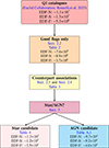 |
Fig. 1. Sketch outlining the steps adopted in this work to attain the AGN candidate catalogues. We report the number of stellar and AGN candidates for the magnitude range 18 < IE ≤ 24.5. |
Euclid Q1 AGN related papers used in this work.
2. Data and counterpart associations
This section provides an overview of the data utilised in this study and the nearest-neighbour matching we perform to identify Euclid’s multi-wavelength counterparts. We begin with a concise summary of the Q1 catalogues, which serve as the foundation for our AGN catalogue. Subsequently, we split the external data into photometry and spectroscopy, detailing the respective instruments and surveys used.
2.1. Euclid Q1 data
Euclid is scheduled to have three major data releases (DRs) over its 6-year nominal mission duration. Detailed descriptions of these releases, as well as information about the mission, are available in Euclid Collaboration: Mellier et al. (2025). However, in addition to the primary releases, there are also interspersed quick releases of smaller volume planned between them. The first of these, the Q1, signifies the initial public release to the scientific community. Details on the data available for the Q1 release can be found in Euclid Collaboration: Aussel et al. (2026), Euclid Collaboration: McCracken et al. (2026), Euclid Collaboration: Polenta et al. (2026), and Euclid Collaboration: Altieri et al. (in prep.).
Q1 encompasses a range of data products. Of particular significance for this study are the photometric catalogues generated by the Euclid MERge Processing Function (MER, Euclid Collaboration: Romelli et al. 2026), which include aperture flux measurements with the corresponding errors, quality flags, and morphological information, as well as template fit and Sérsic fit fluxes in each band for all sources detected in the EDFs. Moreover, Q1 includes imaging (Euclid Collaboration: McCracken et al. 2026; Euclid Collaboration: Polenta et al. 2026) and spectroscopic data (Euclid Collaboration: Copin et al. 2026; Euclid Collaboration: Le Brun et al. 2026), as well as physical parameter estimations (Euclid Collaboration: Tucci et al. 2026).
All EDFs have been observed by the four Euclid photometric bands, i.e. IE from VIS in the visible (Euclid Collaboration: Cropper et al. 2025), and YE, JE, and HE from NISP in the NIR (Euclid Collaboration: Schirmer et al. 2022; Euclid Collaboration: Jahnke et al. 2025). Moreover, as part of the official Euclid data products, the VIS and NISP measurements are accompanied by ground-based optical photometry taken with the ugriz bands of various instruments, including the Ultraviolet Near-Infrared Optical Northern Survey (UNIONS1, Gwyn et al., in prep.) and the Dark Energy Survey (DES, Abbott et al. 2018), that are re-processed through the official Euclid pipelines and homogenised by MER. The data processing of these bands and the breakdown of the resulting available photometry for each EDF can be found in Euclid Collaboration: Aussel et al. (2026).
Additional to the photometric information provided by the Euclid catalogues, Q1 also provides spectroscopic catalogues. These data are obtained from NISP-S observations in two red grisms (RGS000 and RGS180) covering the 1206–1892 nm wavelength range. The data reduction process, spectral extractions and data specifics for Q1 spectroscopy are described in Euclid Collaboration: Copin et al. (2026) and Euclid Collaboration: Le Brun et al. (2026). However, in this work we focus on the Euclid MER photometric catalogues to investigate the source populations present in the Q1 data.
2.2. Quality flags and data cleaning
The Q1 photometric catalogues include a number of artefacts, easily identified through a series of flags that are provided as data models. For instance, the reference photometric measurement of a source is given by the FLUXDETECTIONTOTAL column, and the reliability of this measurement can be assessed using the binary DETQUALITYFLAG column. With this flag, a source can be identified as contaminated by close neighbours, bad pixels, blending with other sources, saturation, being close to a CCD border, being within the VIS or NIR bright star masks, being within an extended object area, or being skipped by the de-blending algorithm. The DETQUALITYFLAG is the most informative flag we use to clean the data from the contaminants listed above. Nevertheless, several other flags can also be used to detect contamination in specific bands (i.e. using < band> _FLAG) or contamination by spurious sources (SPURIOUSFLAG).
In the process of constructing our AGN catalogue from the existing MER Q1 catalogues, we retained only those sources that met our ‘good flags’ criteria:
-
SPURIOUSFLAG = 0,
-
< band> _FLAG = 0,
-
DETQUALITYFLAG = 0| 2| 512.
Here, DETQUALITYFLAG values of 0, 2, and 512 respectively indicate no problems with the data, sources blended together, and sources within an extended object area.
By applying this ‘good flags’ method, we excluded approximately 32% of the data, resulting in what we from now on refer to as the ‘quality-filtered’ catalogues. Furthermore, considering the varying magnitude limits of the external catalogues we use, we refine the data by dividing them into three magnitude bins: 18 < IE ≤ 21, 21 < IE ≤ 22, and 22 < IE < 24.5. A detailed breakdown of the number of sources left after these cleaning steps and splitting of the data is provided in Table 2.
Right ascension and declination of each EDF from Euclid Collaboration: Aussel et al. (2026) and their respective number of sources and impact of quality cuts.
2.3. Photometry
In the following sections we discuss the multi-wavelength photometric data used to identify the different source populations, and the counterpart associations performed in this work, ordered by descending energy. Positional matches with the external surveys were performed using the STIL Tool Set (STILTS version 3.5-1, Taylor 2006), which is a package for command-line processing of tabular data, such as astronomical tables. The matches for the three Q1 fields were tailored to account for their different survey coverages. Table 3 indicates the data sets matched to each EDF, the numbers of sources per data set that fall within the Q1 fields, and the number of counterparts found for the quality-filtered versions of the Q1 catalogues.
Surveys cross-matched per Euclid field.
2.3.1. Ultraviolet
The UV regime offers insights into some of the most active processes in the Universe that are not observable with optical bands. In this energy range, the EDFs overlap with NASA’s Galaxy Evolution Explorer (GALEX, Bianchi 1999). GALEX imaged the sky in two ultraviolet bands: the far-UV (FUV, λeff = 1528 Å); and the near-UV (NUV, λeff ∼ 2310 Å). It provided the first UV sky surveys using two observing modes: direct imaging and grism field spectroscopy. GALEX achieved an image full width half maximum (FWHM) of 4 2 in the FUV and 5
 3 in the NUV. The GALEX GR6/7 data release (Bianchi et al. 2017) includes millions of source measurements, mostly from the All-Sky Imaging Survey (AIS), with a 5σ limiting magnitude of about 20 in FUV and ∼21 in NUV. In this work, we use the combined photoobj catalogue, which includes all GALEX programmes: AIS, Medium Imaging survey (MIS), and the Deep Imaging Survey (DIS). GALEX has a lower angular resolution compared to Euclid’s VIS point spread function (PSF) FWHM of 0
 13 (Euclid Collaboration: Mellier et al. 2025). Therefore, when matching between Euclid and GALEX, we set the fixed error radius in STILTS to a conservative value of 1
 5. This allowed for a more flexible matching, which in itself is important because sources that might have appeared as blended for the GALEX survey can potentially be disentangled with Euclid’s resolution. The total number of matches we obtained between GALEX and the quality-filtered catalogues is 341 222 (see Table 3 for the breakdown of matches per EDF).
2.3.2. Optical
Historically, optical surveys have been significant for identifying and cataloguing a vast number of sources, therefore enhancing knowledge of the Universe and the populations found within it. In this energy range, all three EDFs overlap with ESA’s Gaia mission (Gaia Collaboration 2016). Gaia, with its PSF FWHM of 0 1, aims to measure the three-dimensional spatial and the three-dimensional velocity distribution of stars in order to map and understand the formation, structure, and evolution of our Galaxy. The most recent Gaia Data Release 3 (DR3, Gaia Collaboration 2023a) provides comprehensive source lists that include celestial positions, proper motions, parallaxes, and broadband photometry in the G, GBP (330–680 nm), and GRP (630–1050 nm) passbands, with a limiting depth of G ≈ 21. Additionally, it offers astrophysical parameters and source class probabilities, including stars, galaxies, and quasars (QSOs) over the entire sky. The Q1 catalogues include Gaia IDs from matches performed within the Euclid pipeline, which are released as part of the overall Q1 products. The matching performed between these two surveys is explained in Euclid Collaboration: Romelli et al. (2026), hereafter referred to as RE25. The number of identified matches between the quality-filtered Euclid catalogues and Gaia is 93 198, the breakdown of which is reported in Table 3.
Moreover, the EDF-S and EDF-F share coverage with the Dark Energy Survey (DES, The Dark Energy Survey Collaboration 2005), which is a ground-based visible and near-infrared imaging survey, aiming to cover 5000 deg2 of the southern high Galactic latitude sky. The second DES large data release (DR2, Abbott et al. 2021) contains co-added images and source catalogues, as well as calibrated single-epoch CCD images, from the processing of all six years of DES wide-area survey observations in five broad photometric bands, grizY (Kessler et al. 2015) and all five years of DES supernova survey observations in the griz bands (Diehl et al. 2019), with a detection limit of g < 25 and a PSF FWHM typically around 0 8 (Abbott et al. 2021). To perform the counterpart associations between Euclid and DES, after investigating different fixed error radii based on the PSF FWHM of both surveys, we set this parameter to 0
 55 and obtain a total of 4 528 069 matches (see Table 3 for the breakdown of matches per EDF).
2.3.3. Infrared
The infrared regime provides valuable insights into regions of the Universe that are obscured by dust. In this energy range, the Q1 photometry can be combined with various surveys to enhance our understanding of obscured sources.
In the mid-infrared (MIR), the Wide-field Infrared Survey Explorer (WISE; Wright et al. 2010) is a survey mapping the entire sky in four infrared bands (i.e. W1, W2, W3, W4) centred at 3.4, 4.6, 12, and 22 μm. Its AllWISE programme (Cutri et al. 2013) combined data from the WISE cryogenic and NEOWISE post-cryogenic survey (Mainzer et al. 2011) to form the most comprehensive view of the full mid-infrared sky currently available. The AllWISE Data Release, whose survey maps the entire sky and therefore includes all three EDFs, provides images with a pixel scale of 1 375, source catalogues, multi-epoch photometry catalogues, and reject catalogues up to a detection limit of W1 < 17.1. Similar to GALEX, the WISE-AllWISE resolution is not as powerful as that of Euclid, having a PSF with FWHM of 6
 1, 6
1, 6 8, 7
8, 7 4, and 12″, for its four W1, W2, W3, and W4 bands (Wright et al. 2010). Therefore, when matching between the two surveys, we decided to set the fixed error radius to a conservative value of 1
 5, allowing for a more flexible matching and resulting in a total number of 681 699 matches, the breakdown of which is reported in Table 3.
To further complement the Euclid catalogues, Euclid Collaboration: Bisigello et al. (2026), from now on referred to as BL25, performed forced photometry on Spitzer IRAC images at the position of the Euclid sources (i.e. fixed positions). Briefly, starting from the public images by Euclid Collaboration: Moneti et al. (2022) in all four IRAC bands, which include the [3.6], [4.5], [5.6], and [8.0] filters, they first remove the sky background, using a 3 × 3 pixel filter. Then, the extraction is performed using the position of all Euclid sources, both VIS- and NISP- detected, using an aperture with 1″ radius, resulting in IRAC aperture photometry, which they correct to total, for every Euclid source, therefore making the counterpart association unnecessary.
2.4. Spectroscopy
The following sections discuss the spectroscopic data used to identify the different source populations, and the counterpart associations performed in this work.
2.4.1. DESI EDR
The Dark Energy Spectroscopic Instrument (DESI) is a multi-object fibre spectrograph installed at the Mayall-Telescope at Kitt Peak (DESI Collaboration 2022), capable of covering a 3 2 wide field of view (Silber et al. 2023). In preparation for its ambitious main survey, a set of survey validation projects (DESI Collaboration 2024a) were conducted with DESI to optimise the final target selection and explore the capabilities and limits of the instrument. These tests consisted of a commissioning data set and a series of survey validations (SV) 1, 2, and 3 (Alexander et al. 2023; Brodzeller et al. 2023; Guy et al. 2023; Lan et al. 2023). The data collected during these pilot surveys were published as the early data release (EDR) of DESI (DESI Collaboration 2024b). It contains spectra of 2 847 435 unique pointings (including sky), which yield 1 202 846 reliable extragalactic spectroscopic redshifts.
Since the DESI survey is based on optical ground-based data, it has a spatial resolution of roughly 1″. For its counterpart association, we started by investigating the entire DESI EDR catalogue (DESI Collaboration 2024b), to which we applied the following set of selection criteria to obtain a subsample of objects with robust spectroscopic redshifts:
-
objtype = TGT;
-
deltachi2 > 10;
-
zcat_primary = 1;
-
coadd_fiberstatus = 0;
-
zwarn < 4.
Furthermore, only spectra with good model fits and no serious issues with the redshift determination were used.
Out of the three EDFs, only the EDF-N overlaps with the DESI EDR. To obtain the counterparts, we set the maximum error to 1″ based on DESI’s spatial resolution, and obtain a total number of 64 039 matches with the raw MER catalogues. After applying the quality cuts specified in sect. 2.2, this number is reduced to 24 922 matches between DESI EDR and the quality-filtered EDF-N catalogue.
All the matched DESI spectra belong to the SV3 sample of the DESI EDR, which was covered by a larger number of passes than the yet to be released main survey of DESI. This means that these regions have a higher completeness and at times, due to stacking, deeper observations than what we can expect from the DESI main survey.
2.4.2. SDSS DR17
The Sloan Digital Sky Survey (SDSS; York et al. 2000) is a large-scale imaging and multi-fibre spectroscopic redshift survey that has mapped millions of objects from our Galaxy to the distant Universe, including stars, galaxies, and quasars. Data Release 17 (DR17) of SDSS marks they survey’s fifth and final release from the fourth phase (Abdurro’uf et al. 2022). DR17 contains the entire release of the Mapping Nearby Galaxies at APO Survey (MaNGA, Bundy et al. 2015) as well as the MaNGA Stellar Library and the complete release of the Apache Point Observatory Galactic Evolution Experiment 2 survey (APOGEE; Majewski et al. 2017). Moreover, DR17 also includes data from the SPectroscopic IDentification of ERosita Survey subsurvey (SPIDERS, Clerc et al. 2016; Dwelly et al. 2017) and the eBOSS-RM programme (Shen et al. 2015), as well as 25 new or updated value-added catalogues, covering a total of 14 555 deg2 with an average PSF FWHM, typically measured in the r band, of around 1 3, and an approximate magnitude limit of around r = 22.7 (Blanton et al. 2017; Abdurro’uf et al. 2022). DR17 includes approximately 1.5 million unique spectra for sources, with available spectroscopic redshifts. The SDSS DR17 overlaps solely with the EDF-N, and even then, only a limited number of sources fall within this area. Nevertheless, we conduct a cross-match with the quality-filtered EDF-N catalogue using a fixed radius of
  , based on SDSS’ PSF FWHM, and obtain a total of 18 counterparts.
2.4.3. Other spectroscopic surveys
Gaia DR3 announced a sample of 6.6 million quasar candidates (the qso_candidates table2; Gaia Collaboration 2023a,b), which has high completeness thanks to the combination of several different classification modules, including the Discrete Source Classifier (DSC), the Quasar Classifier (QSOC), the variability classification module, the surface brightness profile module, and the Gaia DR3 Celestial Reference Frame source table. Nevertheless, the Gaia DR3 QSO candidate catalogue has an estimated low purity of quasars (52%) and a large scatter of redshift estimates.
Instead of using the original Gaia DR3 QSO candidates catalogue, we take a purified version to find Euclid counterparts of the sources. This purified catalogue includes: (i) Quaia (Storey-Fisher et al. 2024), with nearly 1.3 million sources at G < 20.5; (ii) CatNorth (Fu et al. 2024), with more than 1.5 million sources down to the Gaia limiting magnitude in the 3π sky of the Pan-STARRS1 (PS1; Chambers et al. 2016) footprint (δ > −30°); and (iii) CatSouth (Fu et al. 2025), with 0.9 million sources with G < 21.0 covered by the fourth data release (DR4) of the SkyMapper Southern Survey (SMSS; δ ≲ 16°; Onken et al. 2024). The compilation of the three catalogues contains more than 1.9 million unique (with unique Gaia sourceid) quasar candidates in the entire sky. This catalogue from now on is referred to as the ‘purified’ GDR3 QSO candidate sample (GDR3-QSOs). We cross-matched the Euclid fields with this integrated GDR3-QSOs catalogue using the Q1 provided Gaia IDs and find 647, 811, and 513 matches in quality-filtered EDF-N, EDF-S, and EDF-F, respectively.
3. Identified populations
In this section, we present the two main populations identified in the Euclid data for this work: stars and AGN. While the primary objective is to investigate various diagnostics for compiling a comprehensive AGN candidate catalogue, stars significantly contribute to the contamination of AGN selection techniques. Therefore, developing an effective selection method to identify the stellar population within the Q1 data is crucial.
To identify AGN, we use traditional colour selection techniques and investigate new colour diagnostics using the limited labelled data obtained after cross-matching the Euclid catalogues. Additionally, we refer to other Q1 papers that also explore AGN detection techniques (see Table 1). All these approaches include using a combination of Euclid’s photometry, photometric and spectroscopic information from the matched data sets, spectral energy distributions (SEDs) fitting, morphological analysis, and machine-learning techniques.
However, despite the cross-matching between the various data sets and Euclid, we lack a substantial number of reliably labelled sources, excluding those from DESI. Consequently, we are unable to accurately quantify the purity and completeness of some of these methods. Follow-up work is necessary to further test the methodologies described here and to accurately quantify these parameters.
For the AGN diagnostics based on Euclid’s photometry (which include the ugriz bands from UNIONS and DES), we use the template-fit fluxes provided by the Q1 catalogues. These fluxes are colour corrected, following the prescription outlined in the MER Data Product Description Document3.
Additionally, we examined the impact of correcting the fluxes for Galactic extinction using E(B − V) values from the Galactic dust map from Planck Collaboration XI (2014). As shown in Galametz et al. (2017), the colour of the source spectral energy distribution (SED) can lead to significant correction variations. We explored extinction corrections for two extreme cases, namely, blackbody temperatures of 100 000 K and 5700 K. As the Galactic latitudes of the EDFs were selected to be in regions of low Galactic extinction, we find that these corrections have a minimal effect on the template-fit fluxes (approximately 5% variation). Consequently, we decided not to implement them.
3.1. Stellar candidates
The proper motion and parallax of an object track its apparent transverse movement over time, as well as its shift in position against a distant background when viewed from different angles. Most stars within our Galaxy show measurable proper motions and parallaxes due to their proximity to us. Vice versa, distant objects like quasars or galaxies have negligible proper motions and parallaxes. Therefore, tracking these two parameters is crucial when attempting to identify stars.
Gaia DR3 provides parallaxes and proper motions for around 1.46 billion sources, with a limiting magnitude of about G ≈ 21 and a bright limit of about G ≈ 3 (Gaia Collaboration 2023a). By identifying the Gaia counterparts and utilising the information provided by Gaia DR3, we have the necessary data to identify as stellar candidates those sources with significant proper motion and parallaxes. However, since the detection limit of Gaia (G < 21) is not as deep as that of Euclid (IE ≤ 26.2), for sources beyond G ≥ 21, an alternative method is required for detecting stellar candidates.
The Q1 data release also includes catalogues with object classifications that provide the probabilities of an object being a star, a galaxy, or a QSO based on the source’s photometry. This is obtained by performing a supervised machine-learning method called probabilistic random forest (PRF; Reis et al. 2019). Specifics on the method used can be found in Euclid Collaboration: Tucci et al. (2026), from now on referred to as TM25. To summarise, the classifiers estimate the probability of objects belonging to a particular class and set a threshold that must be surpassed for an object to be classified into one of the groups. The advised threshold for objects to be considered as stars differs between EDF-N, EDF-S, and EDF-F, with values of 0.58, 0.68, and 0.68, respectively. Upon investigating the data, we decided that a threshold of 0.7 for all three fields provides a purer sample of stellar candidates
By combining information from both Gaia and the Q1 PRF, we are able to construct a comprehensive approach for identifying stellar candidates. However, to refine the star selection and ensure that no extended objects are recorded to have large proper motions and/or parallaxes, or are misclassified by the random forest, we impose an additional condition on the morphology to select only star-like objects. Therefore, only point-like sources (i.e. MUMAXMINUSMAG < −2.6) are considered stellar candidates (Euclid Collaboration: Romelli et al. 2026).
The parameter MUMAXMINUSMAG is the difference between two quantities, both of which are available in the Q1 catalogue: a global measure named MAGSTARGALSEP and a local one named MUMAX. The first is the magnitude used to compute point-like probability, and the second is the peak surface brightness above the background detection level. We note that MUMAX measures the brightest, most concentrated light within a specific area of the source, and MUMAXMINUSMAG is useful for identifying point-sources or nearly point-like sources (Euclid Collaboration: Romelli et al. 2026). Figure 2 indicates how this cut in the data set (MUMAXMINUSMAG < − 2.6) is able to capture the sources that have a high probability of being a point-like source.
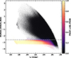 |
Fig. 2. Parameter of MUMAX_MINUS_MAG versus IE for sources in the EDF-N. The colour scale indicates the point like probability of a source. The dotted line indicates the threshold (MUMAX_MINUS_MAG < −2.6) below which most sources appear to be point-like. |
As a result, we adopted the following prescription to select stellar candidates,
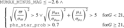 (1)
(1)
where ϖ stands for the parallax of an object, σϖ the error of this measurement, and (μα*, μδ) are the proper motion measured in the right ascension and declination positions, with their corresponding errors, (σμα*, σμδ). We refer to these selected sources as stellarcandidates. Table 4 gives a summary of the number of stellar candidates that we identify in each of the three Q1 fields.
Number of selected stellar candidates per Q1 fields.
3.2. AGN candidates: Photometric selection
We now present different AGN selections applied to the Q1 fields. This initial section examines previously established photometric criteria and introduces novel photometric diagnostics developed for this work. We report the number of AGN candidates recorded per criterion in Table A.1.
3.2.1. Probabilistic random forest
As outlined in Sect. 3.1, Q1 provides object classification catalogues with the probabilities of an object being a star, galaxy, or QSO, obtained using a PRF (TM25). They also provide the probability threshold to use in order to select different populations of sources. In particular, the recommended thresholds for QSOs are 0.67, 0.85, and 0.85 for the EDF-N, EDF-S, and EDF-F, respectively. When investigating the data we decided that a threshold of 0.85 for the EDF-N, and 0.95 for the EDF-S and EDF-F created an overall more refined sample of QSOs. However, since the PRF is trained using photometry only, to avoid contaminants from stellar objects that might have QSO-like colours, we also exclude the stars identified by Sect. 3.1 from the refined sample. We refer to this ‘purified’ version of the TM25 catalogue as the PRF candidates. The total number of identified QSO candidates with this recipe in the quality-filtered catalogues is 180 666, and the breakdown per field is reported in Table A.1.
3.2.2. Bisigello+24 selections
In preparation for the Euclid mission, Euclid Collaboration: Bisigello et al. (2024), from now on referred to as BL24, identified various colour-colour selection criteria for AGN using Euclid photometry alone, and combinations of Euclid photometry with additional external photometric bands. Their study was carried out for both, the EWS and the EDS, using simulated data from the Spectro-Photometric Realisations of IR-Selected Targets at all-z (Spritz, Bisigello et al. 2021). Selection criteria were identified by maximising the F1-score – the harmonic mean of the completeness (C, the fraction of true AGN recovered from the original AGN sample) and the purity (P, the fraction of true AGN among all AGN candidates).
In this work, due to the depth of the MER catalogues, we use the diagnostics derived for the EWS. It is worth noting that all selection criteria developed in BL24 assumed that stars had been previously selected and removed from the sample. Therefore, we remove all stellar candidates identified in Sect. 3.1.
We then apply their purest selection criterion in the EWS to identify QSO candidates based on three Euclid filters. This selection provided them with an F1 score of 0.224 ± 0.001, and was derived from a low purity (P = 0.166 ± 0.015), as well as a low completeness (C = 0.347 ± 0.004). This particular selection follows the prescription
![Mathematical equation: $$ \begin{aligned} \left(I_{\rm E}-Y_{\rm E}<0.5 \right)&, \left(I_{\rm E}-J_{\rm E}<0.7 \right) \nonumber \\&, \left[I_{\rm E}-J_{\rm E} < -2.1 (I_{\rm E}-Y_{\rm E})+0.9 \right]. \end{aligned} $$](/articles/aa/full_html/2026/07/aa54619-25/aa54619-25-eq23.gif) (2)
(2)
This criterion identifies a total of 521 252 QSO candidates in the EDF-N, 755 032 in the EDF-S, and 315 683 in the EDF-F.
In addition to stars, based on the large number of candidates obtained and the low purity of this selection, it is possible that other contaminants also affect this selection. Therefore, to improve the purity of this diagnostic, which was specifically designed to identify unobscured AGN, also referred to as Type I AGN, we impose an additional requirement of point-likeness to eliminate potential extended contaminants (i.e. MUMAXMINUSMAG ≤ − 2.6). This criterion removes approximately 87% of candidates in each field, indicating that many of the initial candidates were extended sources. However, by applying this additional morphological filter, we exclude several AGN at z ≤ 1.2 that may appear as extended sources due to Euclid’s resolution.
Although it is challenging to assess how this additional condition might enhance the purity of the selection, this approach is a straightforward method to further clean the candidate sample without deviating from the prescription established by BL24. The combination of selecting sources with Eq. 2 and MUMAXMINUSMAG ≤ − 2.6 is referred to as selection ‘B24A’ from hereon. The total number of QSO candidates obtained in the quality-filtered catalogues after applying the B24A selection is 211 797, the breakdown of which is reported in Table A.1. Furthermore, Fig. 3 illustrates the QSO candidates selected with B24A in the EDF-N, showcasing the colours of all quality-filtered compact sources in this colour-colour plane and highlighting the QSOs selected as candidates.
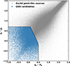 |
Fig. 3. Selection criteria of B24A applied to the EDF-N. In grey we show all quality-filtered Euclid compact sources, while the QSO candidates are shown in blue. We also showcase, with the black dotted line, the limit of the B24A selection. |
BL24 also included some additional diagnostics designed to combine the Euclid photometry with that of other surveys. Specifically focussing on future surveys, such as Rubin/LSST, they characterised a series of criteria using the ugriz bands. Since the Euclid photometry is accompanied by ancillary ground-based optical photometry taken with these bands (details in RE25), we opt to test the selection criteria derived using the u and z bands.
This specific selection follows the prescription
![Mathematical equation: $$ \begin{aligned} \left(I_{\rm E}-H_{\rm E}<1.1\right)&, \left(u-z <1.2\right)\nonumber \\&, \left[I_{\rm E}-H_{\rm E} < -1.3(u-z)+1.9\right], \end{aligned} $$](/articles/aa/full_html/2026/07/aa54619-25/aa54619-25-eq24.gif) (3)
(3)
and it was designed to identify Type I AGN, assuming all stellar candidates had already been removed from the samples. For this selection, BL24 obtained F1 = 0.861 ± 0.004, with C = 0.813 ± 0.011 and P = 0.922 ± 0.017, making it the purest and most complete selection of their work. The EDF-N is the only Q1 field that contains the u band as part of the Euclid ancillary data. Therefore we could only apply this selection to the EDF-N, obtaining a total of 1 092 763 QSO candidates.
Similarly to B24A, we suspect that the large number of candidates might be attributed to potential contaminants infiltrating this selection. Consequently, driven by these other contaminants, we apply the same morphological cut to this criterion. We refer to the combination of Eq. (3) and MUMAXMINUSMAG ≤ − 2.6 as the B24B selection. Applying this combination reduces the number of selected QSO candidates to 114 145. We report this number, split into magnitude bins, in Table A.1. Additionally, fig. 4 illustrates the QSO candidates selected with B24B in the EDF-N, showcasing the colours of all quality-filtered point-like sources and highlighting the QSOs selected as candidates. Once again, it is not possible to assess how the additional condition on morphology might impact the purity of the selection, but this approach provides a way of further cleaning the candidate sample without having to alter the BL24 criterion.
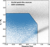 |
Fig. 4. Selection criteria of B24B applied to the EDF-N. In grey we show all quality-filtered Euclid point-like sources, while the QSO candidates are shown in blue. We also showcase, with the black dotted line, the limit of the B24B selection. |
3.2.3. WISE-AllWISE selection
Utilising the supplementary photometry derived from the WISE-AllWISE counterparts, we implement the selection criteria established by Assef et al. (2018), hereinafter called A18. In their work, a series of diagnostics with varying completeness and reliability are examined. For the purpose of this paper, we mainly focussed on their C75 and R90 selection methods. As their names suggest, these criteria were designed to generate catalogues with 75% completeness and 90% reliability, whereby reliability measures the purity of the selection. The completeness-optimised AGN diagnostic is defined by
 (4)
(4)
where the completeness fractions for a given W1 − W2 colour cut are independent of magnitude. Meanwhile, the reliability driven AGN selection takes the form
![Mathematical equation: $$ \begin{aligned} \begin{aligned} \mathrm {W}1 - \mathrm {W}2 > {\left\{ \begin{array}{ll} 0.65\, \mathrm {exp} [{0.153(W2-13.86)^2]}&, \text{ for} \, W2>13.86,\\ 0.65&, \text{ for} \, W2 \le 13.86.\\ \end{array}\right.} \end{aligned} \end{aligned} $$](/articles/aa/full_html/2026/07/aa54619-25/aa54619-25-eq26.gif) (5)
(5)
Additionally, to maintain the completeness and reliability of these diagnostics, it is essential to impose extra conditions, such as W1 > 8, W2 > 9, (S/N)W2 > 5, and the WISE-AllWISE quality flags ccflags = 0. Both of these selections are established for the Vega magnitude system.
Before applying either one of these selections, we remove the stellar candidates identified with the Sect. 3.1 prescription. The total numbers of C75 and R90 AGN candidates is 65 083 and 4688, respectively, and the numbers of AGN candidates per field are reported in Table A.1. Figure 5 shows both of these selections applied to EDF-N sources, where we include all Euclid sources matched to WISE-AllWISE and we highlight those sources that are selected as AGN candidates by C75 or R90.
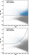 |
Fig. 5. WISE-AllWISE AGN candidates in the EDF-N defined by Eq. (4) (top panel) and Eq. (5) (bottom panel). In grey we show all Euclid sources with WISE-AllWISE counterparts, while the blue sources represent the selected AGN candidates. The black dotted lines represent the limits of the C75 and R90 selections. The stellar candidates have already been removed from the samples of AGN candidates. |
3.2.4. Gaia DR3
Using the Gaia DR3 cross-match data, we identify sources marked as QSO candidates from the GR3-QSOs sample. Specifically, we identify 647, 811, and 513 candidates in the quality-filtered catalogues of EDF-N, EDF-S, and EDF-F, respectively. To address potential stellar contamination within this sample, we exclude the very few sources classified as stellar candidates according to Sect. 3.1. The refined number of sources in the quality-filtered catalogues is presented in Table A.1.
3.2.5. New Euclid-only colour cut: JH_IEY
Euclid provides us with a myriad of information that can be utilised for selecting QSO candidates. Motivated to obtain a purer QSO selection, we investigate a new diagnostic using all four Euclid bands, starting with a morphological cut. Focusing on QSOs, we consider only point-like sources with MUMAXMINUSMAG ≤ − 2.6. Imposing this restriction allowed us to exclude all extended sources that could act as contaminants in our selection at the expense of detectable AGN within extended host galaxies (see Sects. 3.2.3, 3.3, and 3.4).
Subsequently, we created a smaller ‘ground truth’ catalogue where we include sources that have been matched to DESI and have been classed as DESI QSOs while possessing broad-line detection and zspec (see Sect. 3.3). In this way, we are able to differentiate between objects that have a good reliability of being QSOs, galaxies, or stellar candidates.
Imposing good photometry on all sources (i.e. working with the quality-filtered catalogues), we explore the colour–colour space JE − HE versus IE − YE. We identify a cut that excludes the stellar locus, and obtain the following criteria:
![Mathematical equation: $$ \begin{aligned} \begin{aligned} \left[-0.1\le (I_{\rm E}-Y_{\rm E}) <1.0\right]&, [-0.5 \le (J_{\rm E}- H_{\rm E}) < 0.6] \\&, \{ [(J_{\rm E}- H_{\rm E}) > 0.5(I_{\rm E}-Y_{\rm E}) - 0.20] \\&\vee [(J_{\rm E}-H_{\rm E}) > 0.13] \}. \end{aligned} \end{aligned} $$](/articles/aa/full_html/2026/07/aa54619-25/aa54619-25-eq27.gif) (6)
(6)
We then investigated the confusion matrix, completeness and purity in two zspec bins separated by zspec = 1.6. We limited this analysis to IE < 21 since at fainter magnitudes, galaxy contamination from DESI (especially at z > 1.6) is largely unknown. The confusion matrix was computed applying the following labels to the ‘ground truth’ sample:
-
True: DESI QSO labelled objects with a detected broad-line and spec-z are classified as broad-line QSOs (BLQSOs).
-
False: Anything that is not classified as a BLQSO acts as contaminants (galaxies, Type II AGN, stars).
Then, depending on whether or not an object is within our colour-colour selection, we assigned the following:
-
‘Positive’ was assigned when the object is compact and within the selection.
-
‘Negative’ was assigned when the object is not point-like or is outside the selection.
We opted to count stellar contaminants across all redshift bins, given that stars can interfere with selection processes at both low and high z. Using the aforementioned prescription, we achieve P = 0.92 with C = 0.63 for the IE < 21 ∧ zspec < 1.6 bin, and P = 0.95 with C = 0.90 for the IE < 21 ∧ zspec > 1.6 bin. Nevertheless, these values should be taken with caution since they cannot be straightforwardly extrapolated to fainter magnitudes, as the presence of numerous contaminants, especially compact galaxies, could significantly reduce the purity and completeness of this selection at fainter magnitudes. Given the lack of sufficiently reliable labels at fainter magnitudes, assessing the impact of contaminants is challenging. Therefore, we consider this selection method particularly effective for our two brightest IE bins (18 < IE ≤ 21 and 21 < IE ≤ 22), while the statistics for the faintest bin (22 < IE < 24.5) remain less constrained. In Appendix B, we illustrate the number of candidates picked up by this selection, split into our three magnitude bins, where it is evident that at fainter magnitudes, the number of candidates is considerably larger, hinting at higher contamination rates.
With this specific criterion, we identify a total of 313 714 QSO candidates, the breakdown of which can be found in Table. A.1. Additionally, Fig. 6 illustrates the application of this colour cut to the EDF-N, highlighting the corresponding point-like sources that served as DESI counterparts and were used to derive this QSO selection criterion, as well as the stellar locus that we identify in Sect. 3.1.
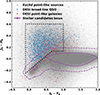 |
Fig. 6. New colour-cut criteria (black dotted line) defined by Eq. (6) applied to EDF-N. In grey we show all Euclid compact sources that have a DESI counterpart. The blue coloured points represent the Euclid compact sources selected as DESI BLQSO candidates and the red ones represent the Euclid compact objects selected as galaxy candidates by DESI. Moreover, the purple lines represent the 68% (solid) and 95% (dashed) contours of the stellar candidates found in Sect. 3.1. |
3.2.6. New Euclid and ancillary photometry colour cut: IEH_gz
Employing Euclid’s ancillary data from Q1, we explore an additional diagnostic using the IE − HE vs. g − z colour space. Similarly to Sect. 3.2.5, we create a smaller ‘ground truth’ catalogue including sources that have been matched to DESI and classed as BLQSOs. We impose the same morphology cut as in Sect. 3.2.5 and we then identify the area occupied by the stellar locus, as well as the locations that the DESI BLQSOs and galaxies populate. Based on this initial realisation, it becomes apparent that it is possible to separate these objects in this colour space with the following prescription:
![Mathematical equation: $$ \begin{aligned} (g-z<1)&, [(g-z < 0.5) , (I_{\rm E}-H_{\rm E}>0.1)]\nonumber \\&\vee [(g-z>0.5) , (I_{\rm E}-H_{\rm E}>(g-z)-0.4)]. \end{aligned} $$](/articles/aa/full_html/2026/07/aa54619-25/aa54619-25-eq28.gif) (7)
(7)
We then followed the same guidelines as the ones presented in Sect. 3.2.5 and investigated the confusion matrix, C and P, in two zspec bins separated by zspec = 1.6, again limiting the analysis to IE < 21. We obtain P = 0.93 with C = 0.60 for IE < 21 ∧ zspec < 1.6, and a P = 0.97 with C = 0.77 for IE < 21 ∧ zspec > 1.6. Once again, given the limited number of labels, particularly at fainter magnitudes, we refrain to assess the performance of this selection at IE > 21. Appendix B illustrates this selection split into the three IE bins to show the increasing number of candidates and therefore contaminants with fainter magnitudes.
With this specific criterion, we identified a total of 267 513 QSO candidates. We show its breakdown in Table A.1. Figure 7 shows the application of this colour cut to the EDF-N, highlighting the corresponding point-like sources that serve as DESI counterparts and which we used to derive this QSO selection criteria.
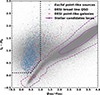 |
Fig. 7. New colour-cut criteria (black dotted line) defined by Eq. (7) applied to EDF-N. In grey we show all Euclid compact sources with that contained a DESI counterpart. The blue coloured points represent the Euclid compact sources selected as DESI BLQSO candidates and the red ones represent the Euclid compact objects selected as galaxy candidates by DESI. Moreover, the purple lines represent the 68% (solid) and 95% (dashed) contours of the stellar candidates found in Sect. 3.1. |
3.3. AGN candidates: Spectroscopic selection
We present the various AGN selections applied to the Q1 fields based on spectroscopy obtained from the DESI counterparts. We report the number of AGN candidates recorded per criterion in Table A.1.
We investigated the presence of QSOs and AGN within the 64 039 matches of DESI EDR to the Euclid matches. We began by creating a subsample of extragalactic objects that only included targeted objects with positive redshifts that had not been spectroscopically selected as DESI stars. To do so, we implemented the following criteria:
-
z > 0.001;
-
SPECTYPE ≠ STAR.
From this subsample, the simplest method for selecting the QSO candidates is by using the DESI spectral type classification (SPECTYPE=QSO, DESI Collaboration 2024b). Additionally, for sources classified as galaxies (SPECTYPE=GALAXY, DESI Collaboration 2024b), we make use of multiple AGN diagnostics based on emission line fluxes, widths, and equivalent widths measured with FastSpecFit (Moustakas et al. 2023). These measurements are available for 40 274 of the DESI EDR-Euclid MER sources.
-
The detection of broad H α, H β, Mg II or C IV emission lines with a FWHM ≥ 1200 km s−1.
-
An AGN classification in the N II ([O III]λ5007/Hβ versus [N II]λ6583/Hα), S II ([O III]λ5007/Hβ versus [S II]λ6717,6731/Hα) or O I ([O III]λ5007/Hβ versus [O I]λ6300) emission line diagnostic diagrams (or ‘BPT diagrams’ after Baldwin et al. 1981, see Fig 8). For the N II BPT, we make use of Kewley et al. (2001), Kauffmann et al. (2003), and Schawinski et al. (2007) to distinguish between AGN, low-ionisation nuclear emission-line region (LINER), composite, and star-formation ionisation. For the S II and O I BPTs, we make use of the Kewley et al. (2006) and Law et al. (2021) limts to distinguish between AGN, LINER and star-formation ionisation.
-
A strong AGN or weak AGN classification in the WHAN diagram of Cid Fernandes et al. (2010), which makes use of the equivalent width of the H α emission line.
-
An AGN classification in the BLUE diagram of Lamareille (2010), which makes use of the equivalent width of the H β and [O II]λ3727 emission lines.
-
An AGN classification in the KEX diagnostic diagram of Zhang & Hao (2018), which makes use of the [O III]λ5007 emission line width.
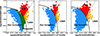 |
Fig. 8. Emission line diagnostic diagram of N II (left), S II (centre), and O I (right) for the Euclid sources with a DESI spectroscopic counterpart. |
Moreover, to identify BLQSOs, we also perform a test to detect broad H α, H β, Mg II, or C IV emission lines with a FWHM ≥ 1200 km s−1 for those sources classed with SPECTYPE=QSO.
This results in a total of 4392 AGN candidates in the quality-filtered catalogue (whereby LINERS identified through the BPT diagnostics are not counted as AGN candidates), the breakdown of which is shown in Table A.1. Additionally, Fig. 8 shows an example of the N II, S II, and O I emission-line diagnostics performed for the DESI counterparts.
3.4. AGN candidates: Other AGN selections
The following AGN diagnostics were developed in other AGN related works conducted in preparation for the Q1 data release (seeTable 1). We report the number of AGN candidates recorded per criterion on Table A.1.
3.4.1. X-rays
Euclid Collaboration: Roster et al. (2026), hereafter referred to as RW25, present the Q1 counterparts to X-ray point sources, starting from the 4XMM-DR14 (Webb et al. 2020), the Chandra Source Catalog (CSC) Release 2 Series (Weisskopf et al. 2002; Evans et al. 2024) and the eROSITA (Predehl et al. 2021) first Data Release (DR1; Merloni et al. 2024). For each of the Q1 fields and each of the X-ray surveys they first identify the best Euclid counterpart by means of the Bayesian algorithm NWAY (Salvato et al. 2018), which assigns the probability of a good association considering a) the separations between sources, their positional uncertainties, and their number density and b) the similarity between the SED of a candidate counterpart and the SED of a typical X-ray emitter, regardless whether the source is Galactic or extragalactic. The latter information is provided by a prior externally defined using a random forest on a set of Euclid-only features (i.e. no features from ground-based photometry) extracted from the Q1 catalogues for a training sample of secure X-ray emitters and secure field sources. The same procedure is repeated, randomizing the coordinates of the X-ray catalogues so that the probability of a chance association can be determined (see RW25 for details).
After the determination of the counterparts, the authors then assign to each source a probability of being Galactic (star, compact object) or extragalactic (galaxy, AGN, QSO). This is again done using a training sample of secure Galactic and extragalactic sources and Euclid-only features from the Q1 catalogues. Finally, for the sources that have a probability larger than 50% of being extragalactic, the authors provide either photometric redshifts computed using PICZL (Roster et al. 2024) on Legacy Survey DR10 (Dey et al. 2019) images (and thus limited to the sources detected in that survey) or spectroscopic redshifts from literature.
The released catalogues enable users to refine their samples based on specific scientific needs, balancing purity and completeness through the NWAY output parameters. In total, they report 12 645 AGN candidates, though some sources have multiple counterparts; when considering only the best match for each unique X-ray source, the sample reduces to 11 286 candidates. They identify 949 in EDF-N, 3789 in EDF-S, and 6548 in EDF-F.
From their catalogue, in order to identify those candidates that have the highest probability of being an AGN candidate, we select a subsample of sources with PGal < 0.2. Implementing our ‘cleaning’ on these candidates we obtain 434, 1812, and 3813 X-ray candidates in the quality-filtered EDF-N, EDF-S, EDF-F catalogues (see Table A.1).
3.4.2. Diffusion models
Euclid Collaboration: Stevens et al. (2026), hereinafter called SG25, use the reconstruction error of a diffusion model, a type of generative model, to select AGN candidates. Through training on VIS images, the model is able to learn a bias for the light profile at the centres of galaxies. Since AGN are rare, the bright pixel and steep fall off of light they exhibit is converted to one that is significantly flatter, leading to a high reconstruction error for suspected AGN. They obtain a total of 15 940 AGN candidates across the three EDFs (see Table A.1).
3.4.3. Deep learning
Euclid Collaboration: Margalef-Bentabol et al. (2026), referred to henceforth as MB25, presents a deep learning method to quantify the AGN contribution (fPSF) of a galaxy using VIS imaging. The deep learning model is trained with a sample of mock images generated from the IlllustrisTNG simulations, designed to mimic Euclid VIS observations, with different levels of AGN contributions artificially injected as PSFs. The deep learning model is trained to estimate the level of the injected PSF, achieving a root mean square error of 0.052 on the test set. After applying this model to the Q1 data, they find 48 840 galaxies across the EDFs that are classified as AGN based on this AGN contribution, that is, fPSF > 0.2. Adopting a less conservative threshold of fPSF > 0.1 increases the number to 158 711 AGN. This method allows for the identification of AGN even when the AGN component is not the primary contributor to the host galaxy’s luminosity. The resulting number of AGN candidates found per field and magnitude bin is in Table A.1.
3.5. AGN fraction from SED fitting
Spectral energy distribution template fitting is a powerful method for measuring the physical properties of galaxies and AGN by reproducing the observed photometry with a combination of theoretical and empirical SED models that account for the different AGN and galaxy emission processes. The result of the multi-component SED fitting constrains a variety of physical properties, notably the AGN fraction, which is defined as the ratio of the AGN flux to the total flux in the MIR band and is used for AGN identification (see e.g. Dale et al. 2014; Thorne et al. 2022). By decomposing the emission from the galaxy and the potential AGN components, SED fitting permits the identification of fainter AGN compared to colour-colour approaches. Moreover, since the IR emission is not significantly impacted by AGN obscuration, SED fitting can reliably identify obscured AGN missed by optical or X-ray methods (Pouliasis et al. 2020; Andonie et al. 2022).
Since accurate redshift measurements are required for reliable SED fitting, we first restricted the analysis to sources with spectroscopic redshift in EDF-N, computing the AGN fraction as the ratio between the AGN flux and the total flux over the 5–20 μm wavelength range (following Dale et al. 2014; Thorne et al. 2022). These results can be used to define an accurate selection threshold for AGN that could later be applied to the entire sample with photometric redshift. We used the SED fitting algorithm CIGALE (Boquien et al. 2019; Yang et al. 2022) to fit the UV-to-mid-IR photometry of our sources, including: GALEX FUV/NUV, ugriz, Gaia-G/BP/RP, EuclidIE/YE/JE/HE, WISE W1/2/3/4. Our modelling consists of a delayed star-formation history with a simple stellar population from Bruzual & Charlot (2003) and the Chabrier (2003) initial mass function, a galactic dust attenuation (Calzetti et al. 2000) and emission (Draine et al. 2014), nebular lines (Inoue 2011), and an AGN model (Fritz et al. 2006). For further details, we refer to Laloux et al. (in prep.), from now on referred to as LB25, which presents the physical properties of the AGN candidates in the three EDFs.
The results are shown in Fig. 9, where the normalised cumulative distribution of the AGN fraction for normal galaxies is compared to the different AGN samples. As indicated by the vertical black dotted line, we define our AGN fraction threshold as the intersection between the normal galaxy distribution (dash-dotted blue line) and the broad-line AGN one (BLAGN, dash-dotted red line), whereby BLAGN refers to those sources classified as QSOs or galaxies that exhibit broad emission lines of Hα, Hβ, Mg II, or C IV. An AGN fraction threshold at fAGN = 0.25 is a compromise between purity and completeness, since it correctly selects 77% of the spectroscopically confirmed BLAGN while only 23% of the non-AGN candidates are misclassified as AGN. With this threshold we obtain a total of 7766 AGN candidates within the quality-filtered catalogues, the breakdown of which can be found in Table A.1. A lower AGN fraction threshold, such as fAGN = 0.1 (Thorne et al. 2022), would lead to an increased AGN completeness (97%), but with a much higher false-detection probability (78%). Conversely, a higher AGN fraction threshold of fAGN = 0.5 improves the purity, with a false-detection probability of 5%, at the expense of the completeness (44%).
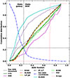 |
Fig. 9. Normalised cumulative distribution of the AGN fraction measured by SED fitting for the different AGN selection methods in EDFN: C75/R90 (green solid/purple dashed), B24A/B (grey/lime dashed), spectroscopically confirmed broad-line or narrow-line AGN (red dash-dotted/cyan solid), IEH_gz (yellow solid), JH_IEY (black dash-dotted), PRF (dark blue dotted, TM25), and X-ray (pink solid,, RW25). The blue dashed-dotted line is the inverse cumulative distribution of all non-AGN candidates. The vertical black solid line represents the proposed AGN fraction threshold (fAGN = 0.25) discriminating AGN and non-AGN sources, while the horizontal black dotted line shows the corresponding false-positive probability (23%). We note that only two X-ray sources have counterparts with zspec in the quality-filtered EDF-N catalogue. |
In Fig. 9, we also compare the AGN fraction distribution for different AGN-selection methods. We find that AGN candidates selected by C75, B24B, IEH_gz, and JH_IEY show a similar AGN fraction distribution to the BLAGN, while the R90 candidates tend to have higher AGN fractions. This suggests that the more reliable methods select sources where the AGN emission dominates over its host, potentially missing weaker AGN. Conversely, the B24A method tends to select sources with lower AGN fractions, some of which are likely to be contaminants, as indicated by the curve of the non-AGN candidates. Additionally, the cyan curve, representing the narrow-line AGN (NLAGN) from the DESI emission-line diagnostics, is significantly shifted to lower AGN fraction values compared to other methods. This demonstrates that while SED fitting is efficient at identifying unobscured AGN, achieving both high completeness and purity for obscured AGN is more challenging. Nevertheless, it still manages to reach 32% completeness for these elusive AGN.
In this section we discussed only qualitatively the comparison of the results of the SED fitting analysis for different selection approaches applied to sub-samples with spectroscopicredshift. The same results will not necessarily hold for samples that only have photometric redshifts, as the availability of a spectroscopic redshift could impact the selections and introduce a bias in the AGN fraction distributions. The AGN fraction from SED fitting for the three deep fields for spectroscopic and photometric redshift sources is provided in LB25.
4. Discussion
4.1. Contaminants
Although Euclid offers exciting prospects for AGN selection, similar to all AGN criteria, several contaminants must be considered when developing these methods. As already discussed in Sect. 3.1, stars are a big contaminant when it comes to colour-colour diagnostics. However, other types of stellar objects also make it hard to create a pure AGN selection technique.
For instance, young stellar objects (YSOs), asymptotic giant branch (AGB) stars, and H II-regions can show very similar colours to those of AGN and therefore slip through the selection criteria as potential candidates. Another form of contaminants, related to low mass products of star formation would be that of brown dwarfs (Davy Kirkpatrick et al. 2011) whose feature at 1 μm can sometimes resemble a Ly α break at redshifts z = 6–7.5 (Wilkins et al. 2014; Hainline et al. 2024; Langeroodi & Hjorth 2023).
Compact normal galaxies can also play a big role as contaminants in AGN diagnostics (Kouzuma & Yamaoka 2010). This is because, at higher redshifts, distant galaxies may appear as point-like sources and show similar colours to that of AGN, therefore contaminating the AGN locus in colour-colour plots. Additionally, dwarf irregulars (Irr) have a 4000 Å break, meaning that, at some redshifts (z < 1), their SEDs are very similar to those of QSOs (BL24). Moreover, high-z star-forming galaxies (SFGs) can sometimes also be considered a contaminant, since their SEDs resemble those of AGN. However, since their 4000 Å break lies within Euclid’s bands at z > 1, it might be easier to separate between AGN and SFGs at these higher redshifts.
These contaminants are likely affecting the colour selections analysed in this work. With our current knowledge and understanding of the Q1 data, we are unable to identify these sources, making it difficult to distinguish between them and potential AGN candidates. Consequently, we acknowledge that, especially at fainter magnitudes, these sources are contaminating our AGN sample, which worsens our calculated values for purity and completeness. Addressing this issue would require further work, such as combining our data with other photometric catalogues that include bands that would facilitate the separation of these objects, or obtaining more spectroscopic data to test for specific emission lines, like those mentioned in Sect. 3.3.
4.2. Comparison to expectations
Prior to this work, Euclid Collaboration: Selwood et al. (2025), from now on addressed as SM25, examined the AGN surface density expected for the Euclid mission. Starting from an X-ray luminosity function (Fotopoulou et al. 2016), they predicted the observational expectations for AGN with z < 7 in the EWS and EDS. They generated volume-limited samples covering 0.01 ≤ z ≤ 7 and 43 ≤ log10(Lbol/erg s−1) ≤ 47. Each AGN was assigned an SED based on its X-ray luminosity and redshift. Dust extinction was applied, and once assigned and scaled, they performed mock observations of each AGN SED in their sample, convolving with the Euclid bands and an assortment of ancillary photometric bands to explore the observable population of z < 7 AGN in the Euclid surveys. They concluded that Euclid should be able to detect significantly more AGN in the EWS and EDS compared to those identified in other surveys covering similar regions. In the EDS they predicted an unobscured AGN surface density of 346 deg−2 based on the BL24 Eq. (2) selection, which is comparable to the densities obtained by Spitzer (Lacy & Sajina 2020) and the XXL–3XLSS (Chiappetti et al. 2018) survey. Similarly, the EWS was estimated to recover an AGN surface density of 331 deg−2, surpassing the AGN densities obtained from both ground-based optical and space-based MIR missions.
We compared the AGN surface densities recovered in 18 < IE ≤ 24.5 and 18 < IE ≤ 22 for each one of the selections investigated in this work against the EWS predictions from SM25, which were based on a 5σ limit in all four Euclid bands, corresponding to a limiting magnitude of IE ≈ 26.2. Starting with the BL24 candidates, in Fig. 10 we observe differences in the surface densities recovered for B24A and B24B. Given that B24B could only be applied to the EDF-N, the area used to calculate its AGN surface density is that of the EDF-N (23.9 deg2), as opposed to the Q1 area (63.1 deg2), which is used for most of the other selections. B24A/B have distinct statistics, with B24A having P ≈ 0.17 and C ≈ 0.35, while B24B has P ≈ 0.92 and C ≈ 0.81. Based on these numbers, the AGN surface densities for both selections align with their expectations. B24A retrieves a greater number of AGN, likely due to its low purity, indicating that a notable amount of contaminants could be identified as candidates. The notably lower AGN surface density obtained for B24B can be attributed to the high purity of this selection, which indicates a smaller number of contaminants. Both selections reveal a significant difference in AGN surface densities recovered in 18 < IE ≤ 24.5 and 18 < IE ≤ 22, highlighting that at fainter magnitudes, we encounter a higher number of contaminants that are difficult to distinguish from actual AGN.
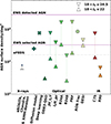 |
Fig. 10. Comparison of AGN surface densities obtained from the selection methods discussed in this work divided into energy bands: X-ray selections (blue), optical selections (shades of green), and IR selections (shades of orange). For the selections B24A, B24B, JH_IEY, IEH_gz, C75, R90, DESI, and PRF, the AGN surface densities are split into 18 < IE ≤ 24.5 (upside down triangles) and 18 < IE ≤ 22 (upside up triangles). For the GDR3-QSOs, only the 18 < IE ≤ 22 is shown due to the limiting magnitude of Gaia. Individual markers indicate AGN surface densities from other Q1 related works, including X-ray candidates from RW25 (with the lower limit indicated by an arrow pointing up); diffusion model candidates from SG25 (plus sign); deep learning candidates from MB25 (cross); and AGN fraction candidates from from LB25 (hexagon). The predictions for the detectable AGN (purple horizontal solid line) and identifiable AGN (purple dashed line) in the EWS from SM25 are included. The grey horizontal dashed line represents recovered AGN surface density by eFEDS (Liu et al. 2022a). |
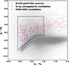 |
Fig. 11. Selection JH versus IEY (black dotted line) applied to the EDF-N. In grey we show all Euclid compact sources. The red coloured dots represent the X-ray selected AGN candidates from RW25, while the purple dots indicate the GDR3-QSOs, which mainly lie within the selection. |
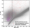 |
Fig. 12. Selection IEH versus gz (black dotted line) applied to the EDF-N. In grey we show all Euclid compact sources. The red coloured dots represent the X-ray selected AGN candidates from RW25, while the purple dots indicate the GDR3-QSOs, which mainly lie within the selection. |
From Fig. 10 it is apparent that the number of AGN selected by the PRF is comparable to those selected by B24A in the range of 18 < IE ≤ 24.5, but it is significantly smaller in the range of 18 < IE ≤ 22. This variation is likely due to the PRF potentially misclassifying compact galaxies with QSOs at fainter magnitudes. The larger number of candidates at fainter magnitudes indicates that, even when we increase the thresholds beyond the recommended values, many contaminants still affect this selection, highlighting that the advised Q1 PRF thresholds are too lenient and should be revised.
The observed numbers for both the C75 and R90 criteria align with what we expected for both of these catalogues. For the C75 criteria, with a completeness of 75%, we anticipated a larger number of candidates, as illustrated in Fig. 10. However, this expectation comes with the potential for an increase in contaminants. By excluding the stellar candidates, we have likely marginally increased the reliability of this selection, though we currently lack the tools to precisely quantify these effects. In contrast, R90 aims to create a more reliable, or purer, catalogue, resulting in a smaller AGN candidate size, as illustrated in Fig. 10. Notably, C75 recovers almost over an order of magnitude more candidates than R90 in both 18 < IE ≤ 24.5 and 18 < IE ≤ 22. Another observation from R90 is that the AGN surface density for 18 < IE ≤ 24.5 and 18 < IE ≤ 22 are not very different from each other, whereas other methods show a significantly higher AGN surface density in the faintest bin. The relatively bright limiting magnitude of this WISE-AllWISE selection (W1 < 17.0 (Vega) = 19.7 (AB)), together with its high purity, makes this selection highly incomplete at faint IE magnitudes, since the number of very red selected candidates (with faint IE magnitude) is small. This effect produces the small increase of the number of candidates going from IE < 22.0 to IE < 24.5.
Both of the new selections, JH_IEY and IEH_gz, recover similar AGN surface densities, which in the 18 < IE ≤ 24.5 appear to surpass the expectations of what is identifiable as an AGN according to SM25. However, the high purity achieved by these selections was only quantified for IE < 21. Therefore, we consider the AGN surface densities recovered in 18 < IE ≤ 22 to be more reliable since we lack the means to assess how the P and C of these selections might change with increasing magnitude. This raises questions about the reliability of the candidates obtained for both selections at IE > 21–22. Further work involving additional galaxy labels or spectra may be necessary to verify whether these AGN surface densities are accurate or inflated by contaminants.
The GDR3-QSO sample was originally quite small compared to the other samples of candidates (1971), so it was expected that the recovered AGN surface density was going to be orders of magnitude lower than that of other surveys. In Fig. 10, we only show GDR3-QSO’s number density for 18 < IE ≤ 22. This is due to the lack of GDR3-QSO candidates at the faintest magnitudes, which is linked to Gaia’s detection limit at G < 21.
DESI only covers a reduced area of the EDF-N, which we calculate to be approximately 9 deg2. We use this area to obtain the corresponding AGN surface density for the sources selected with DESI, which include QSOs, galaxies with detected broad-lines, and AGN selected via BPT or other narrow-line emission diagnostics. We find that the results are consistent with the expectations outlined by SM25 within the range 18 < IE ≤ 22, and exceed the expectations for 18 < IE ≤ 24.5. This is indicative of potential synergies between Euclid and DESI in the future when more data from both survey are available.
We also assess the overall AGN surface density of the X-ray AGN identified by RW25, which is lower than that recovered from eFEDS (Liu et al. 2022b). However, we note that the X-ray catalogue created in RW25 is a combination of different X-ray catalogues with varying depths (see Figure 1 of RW25). Therefore, the surface density reported in Fig. 10 should only be taken as a lower limit, where to estimate the surface area, we generated a multi-order coverage map with a resolution of 6 87, yielding a total area of 36.72 deg2.
We note that the candidates obtained by using the AGN fraction derived from SED fitting surpasses the limit of the identifiable AGN set by SM25. This could be due to SM25’s use of diagnostics specific to unobscured AGN, which, in turn, may have biased their predictions toward the expected detection limits for such type of AGN, rather than capturing both obscured and unobscured populations. In contrast, SED fitting, though not perfect, is more effective at identifying both obscured and unobscured AGN, potentially leading to the higher recovered AGN surface density when using AGN fraction. However, SED fitting is still affected by contaminants, and the quality of the available photometry dictates the quality of the SED fit.
For most of the selections applied in this work, there seems to be a consistent trend. The magnitude range 18 < IE ≤ 24.5 recovers a larger AGN surface density, likely filled with contaminants, while the brightest 18 < IE ≤ 22 bin shows lower densities, usually below the predictions of SM25. Despite the goal of achieving a reliable surface density across all magnitudes, further work is required to assess and enhance the reliability of these selections in the faintest magnitudes. Therefore, we consider the 18 < IE ≤ 22 range to provide a ‘purer’ catalogue of AGN candidates.
The resulting AGN surface density of our selections B24A, B24B, JH_IEY, IEH_gz, GDR3-QSOs, PRF, SED-fitting, and DESI candidates is 3641 deg−2 for 18 < IE ≤ 24.5. By applying this magnitude cut, we eliminate saturated sources from the brightest magnitudes as well as the faintest sources in the Q1 catalogues. We acknowledge that this approach results in missing a population of Euclid sources detectable at a 5σ limit of IE, for which we currently lack the tools to study comprehensively. Given the potential contamination even within this cut, we propose that the purest sample of AGN candidates lies in the magnitude range 18 < IE ≤ 22, resulting in an AGN surface density of 482 deg−2. Even after narrowing the magnitude range of our selection, the AGN surface density recovered remains higher than what was expected to be identifiable with Euclid, yet falls short of the expected number of detectable AGN. This indicates that further refinement of our selection criteria is necessary to bring the number of reliable AGN candidates closer to what should be observable. Notably, this need for improvement is especially critical for Type II AGN, which have been largely excluded from most of the photometric selections evaluated in this study (not including the MIR, X-ray, SED-fitting, and spectroscopic diagnostics). With machine-learning and contributions such as those conducted by SG25 and MB25 we hope to be able to bridge the gap between detected and selected AGN, thereby reducing the bias against Type II AGN that typically arises from most colour-colour selections. In fact, the recovered AGN surface densities from SG25 and MB25, which are limited to IE < 22 and IE < 24.5 respectively, already highlight how effective machine learning can be in thisregard.
4.3. Comparison among AGN selections
In this work, we have examined a variety of AGN diagnostics to construct the first Euclid multi-wavelength catalogue of AGN candidates. However, as expected, most of these AGN selections are incomplete and biased.
Focusing on the photometric selections applied to the Euclid photometry, which include B24A, B24B, JH_IEY, and IEH_gz, it is the IEH_gz diagnostic that achieves the highest purity, with P ≈ 0.93 for zspec < 1.6 and P ≈ 0.97 for zspec > 1.6. However, JH_IEY (P ≈ 0.92 for zspec < 1.6 and P ≈ 0.95 for zspec > 1.6) and B24B (P ∼ 0.92) are only slightly lower. For the new selections, JH_IEY and IEH_gz, the calculation of P and C is limited to IE< 21, thus considering only the brightest sources. This limitation is problematic at the faintest magnitudes, where we cannot assess the P and C values and the effects of different contaminants due to the lack of reliable labels (see Figs. B.3 and B.4).
To determine whether the new selections align with other QSO and AGN candidates, we examine the agreement of these methods with the GDR3-QSO and X-ray AGN candidates. From Fig. , which illustrate the GDR3-QSO and X-ray candidates in the selections JH_IEY and IEH_gz colour spaces, it is evident that both selections agree with the GDR3-QSOs, capturing most of them, while only selecting some of the X-ray sources. This outcome is expected as both of the new selections are designed to select Type I AGN, i.e. QSOs, hence the agreement with GDR3-QSOs, while X-ray samples contain a significant fraction of Type II AGN, which would occupy a different region of the colour space. The agreement with the GDR3-QSOs can also be attributed to the fact that these sources are selected using Gaia information, which has a detection limit of G < 21, therefore somewhat agreeing with the IE < 21 cut we used to calculate the P and C values of selections JH_IEY and IEH_gz.
The issue of contaminants at fainter magnitudes also affects the B24A and B24B selections. At the faintest magnitudes, these selections introduce a large number of candidates that are likely compact galaxies or other types of contaminants, such as brown dwarfs or stellar objects, which cannot be disentangled using colour cuts alone (see Fig. B.1 and B.2).
The DESI-selected QSO and AGN candidates exhibit higher reliability since they utilise DESI spectra from Euclid counterparts to assess the population a source may belong to. We particularly trust those DESI BLQSO candidates, since these are indicative of Type I AGN activity, due to the high velocities of the ionised clouds within the broad-line region (BLR) of an AGN (Antonucci 1993; Veilleux 2002). Moreover, the NLAGN candidates tend to have high reliability because BPT diagnostics use a combination of nebular emission lines to differentiate between various ionisation mechanisms in gas (Baldwin et al. 1981). This helps distinguish between AGN, LINERs, SFGs, and composite objects, which encompass starburst-AGN objects (Kewley et al. 2006). The WHAN, KEX, and BLUE diagrams are similar in the sense that they also use specific line ratios and compare these to source qualities in order to identify different populations. However, although these may be more reliable AGN diagnostics at times, they are still incomplete and biased, and the sources identified with them should still be considered candidates.
For the specifics on the purity and completeness of the GDR3-QSOs, C75, R90, and X-ray selected AGN candidates, as well as those obtained using morphology and machine-learning information, we point the readers to the corresponding papers Storey-Fisher et al. (2024), Fu et al. (2024, 2025), A18, RW25, SG25, TM25, MB25, and LB25.
To assess the overlap among the various selection methods investigated (excluding the morphology-based ones from SG25 and MB25, since their methodologies differ significantly from the other techniques explored in this work), Fig. 13 visualises the portion of AGN candidates identified by multiple selections simultaneously per EDF. To enable a better comparison, we set the detection limit to the range of 18 < IE ≤ 22, ensuring all selections match in depth.
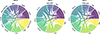 |
Fig. 13. Comparison among the number of sources selected as AGN candidates for the different criteria investigated in this work per EDF. We exclude the morphology-based AGN candidates from SG25 and MB25 due to the significant differences in their methodologies compared to other techniques explored in this work. X-ray candidates correspond to those sources from RW25 and PRF correspond to the purified sample from TM25. We set the detection limit to the range of 18 < IE ≤ 22, ensuring all selections match in depth. We note that EDF-N shows more selection criteria than EDF-S and EDF-F due to the available u-band photometry from UNIONS and spectroscopy from DESI in the EDF-N. |
We find that although most selections overlap to some extent in AGN candidates, there is a large number of candidates that do not co-exist in the different AGN samples. Notably, the PRF, B24A, and JH_IEY selections have substantial portions of their QSO candidate populations that are not selected by other diagnostics, potentially indicating that a number of these sources could be contaminants. Similarly, this behaviour is observed for some C75 candidates. However, the C75 selection is designed to identify AGN in general, which suggests that some of these sources may be Type II AGN, not detectable by the other QSO-specific diagnostics. Potential future work combining Euclid’s photometry with that of WISE-AllWISE could be a promising approach to reduce the bias against Type II AGN. Nevertheless, this lies outside the scope of the current work.
We observe that most of the DESI AGN, GDR3-QSO, and X-ray extragalactic candidates appear to be consistently identified by the other diagnostics. Appendix C provides a numerical representation of Fig. 13 to quantify the agreements between selections.
In total, and including the AGN candidates identified in this work, which include B24A, B24B, JH_IEY, IEH_gz, DESI, PRF, SED-fitting and GDR3-QSOs, our current catalogue includes 229 779 AGN candidates in 18 < IE ≤ 24.5, which is equivalent to an AGN surface density of 3641 deg−2. However, due to contamination, we believe the purest sample of AGN is in the magnitude range 18 < IE ≤ 22, resulting in a total of 30 422 AGN candidates i.e. 482 deg−2. This sample, although primarily composed of Type I AGN, also includes some Type II AGN identified through the DESI and WISE-AllWISE diagnostics.
4.4. Obscured versus unobscured AGN
The majority of the AGN selection methods used in this work are specifically designed to select QSOs. These sources are easier to detect due to their distinct colours and point-like appearance. Additionally, as they are face-on AGN, they are minimally affected by dust, meaning their observed fluxes have not been significantly attenuated. The main drawback of optical photometric selections is that they are heavily affected by dust, making them easily optimised for Type I AGN while being heavily biased against Type II AGN. Despite Euclid having NIR filters, it was predicted that selecting all AGN, including optically obscured AGN and composite systems, would be challenging with Euclid filters alone or supplemented by optical or other bands (BL24).
To ascertain this, we investigate the regions that the DESI spectroscopically selected narrow-line AGN populate in different colour spaces. Figure 14 showcases an example of one of the DESI spectroscopic tests, the N II BPT diagnostic, plotted on the IE − HE versus g − z space. It is apparent that the area populated by the AGN is significantly entangled with that of composite, SFGs, and LINER galaxies, highlighting that obscured AGN do not occupy a specific and distinct region of the colour space. This behaviour was observed for all spectroscopic diagnostics across the different Euclid colour combinations.
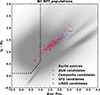 |
Fig. 14. Selection IEH versus gz (black dotted line) applied to the EDF-N. In grey we show all Euclid sources. The blue dots represent the N II selected AGN candidates, the composite galaxies are shown in purple, the SFGs in red and the LINERs in green. |
Moreover we note that out of the total number of DESI broad-line QSOs (1434) 91% are selected by our QSO diagnostics, while from the total of NLAGN selected emission line diagnostics (2761) only 8% are detected by other selections, therefore highlighting the still existing bias against Type II AGN. Additionally, to further demonstrate the differences in populations identified by the spectroscopic and QSO selections, we use the ancillary photometry from the multi-wavelength catalogue to explore the SEDs of the AGN selected by these methods.
We first create a subsample of sources simultaneously identified as QSO candidates by B24A, B24B, JH_IEY, IEH_gz, and DESI BLQSOs, resulting in a total of 279 candidates. For these sources, we perform SED fitting with CIGALE using ancillary optical-to-IR photometric information and DESI’s zspec and examine their best-fit models and corresponding VIS cutouts. Figure. 15 provides an example of the SED fitting and VIS images for two of these selected Type I QSO.
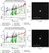 |
Fig. 15. Spectral energy distributions and corresponding VIS cutouts of two QSO candidates identified by the selections JH_IEY, IEH_gz, B24A, B24B and simultaneously classified as broad-line QSOs by DESI. |
The SEDs show a notably strong AGN component in the mid-IR, even dominating the star-formation emission at longer wavelengths for source 2663093395657204902. Linked to the star formation, we also notice moderate dusty absorption on the stellar emission. The corresponding AGN fractions and stellar masses obtained for these sources are approximately 0.46 and M* ≈ 1010.5 M⊙ for source 2703664071644731101 and 0.69 with M* ≈ 1010.1 M⊙ for source 2663093395657204902. The VIS cutouts reveal the point-like appearance of thesecandidates.
We then created a second subsample of sources identified as AGN candidates by either of the DESI narrow-line spectroscopic selections, and similarly fitted their optical-to-IR SED. Figure. 16 showcases the SEDs and VIS cutouts for two of these AGN candidates. The corresponding AGN fractions and stellar masses obtained for these sources are approximately 0.31 and M* ≈ 1010.5 M⊙ for source 2679391751656821227 and 0.97 with M* ≈ 1010.8 M⊙ for source 2661957306668287025. It should be noted that the absence of a WISE-AllWISE counterpart, and therefore photometry, for source 2679391751656821227 results in a large uncertainty (±0.16) in its AGN fraction. The VIS cutouts reveal extended sources with bright centres and, in the case of 2661957306668287025, a dust lane.
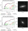 |
Fig. 16. Spectral energy distributions and corresponding VIS cutouts of two narrow-line AGN candidates identified via BPT diagnostics. |
This test highlights the difference between the average unobscured sources selected with our current QSO diagnostics and the obscured sources identified with spectroscopy. This opens an exciting path for future work to exploit similar types of spectroscopic diagnostics on the Euclid spectra to verify if more obscured AGN can be identified using Euclid’s spectroscopic capabilities, notably in extended sources, currently excluded of most QSO-selection approaches.
4.5. Galaxy major mergers with AGN contributions
Euclid Collaboration: La Marca et al. (2026), hereafter LM25 make use of a convolutional neural network (CNN) to perform morphological classification of a stellar mass-complete sample of Q1 galaxies in the redshift range 0.5 ≤ z ≤ 2.0. The CNN is trained with EuclidIE mock observations created from the IllustrisTNG simulations, with different levels of AGN contributions injected in 20% of the sample. The authors classify 113 155 galaxies as mergers and 269 933 as non-mergers. Then, they utilise the AGN catalogues presented in RW25, MB25, and in this work, to select AGN in four different ways (X-ray detections, through the fPSF parameter, optical spectroscopy, and with MIR colours) to study the possible connection of mergers with each AGN type. LM25 observe a larger fraction of AGN in mergers compared to non-mergers, with the largest AGN excess seen in MIR-selected AGN, and a dependence of the merger fraction on the fPSF parameter and the AGN luminosity. Their analysis supports the scenario in which mergers are most closely connected to the most powerful and dust-obscured AGN.
5. The AGN catalogue
The catalogues created in this work (available through Zenodo4 and CDS) contain the counterparts to the Euclid sources from GALEX, Gaia, DES, WISE-AllWISE, DESI, and SDSS with their corresponding IDs, RA, and Dec, and spectroscopic redshifts when available (columns 1–23). We also include the flags to clean the data similarly to our work (column 24), split the data into our magnitude bins (25–27), and identify the stellar candidates (28–30). Additionally, columns 31–47 flag the sources that have been selected as AGN candidates via the various tests conducted in this study, including PRF, B24A, B24B, C75, R90, GDR3-QSOs, JH_IEY, IEH_gz, and the different DESI diagnostics. Finally, we also include the results from the SED fitting explored alongside this work, which includes columns for the AGN fraction of those sources with DESI redshifts, their corresponding errors, and the resulting selected AGN candidates (columns 48–50). A detailed description of the columns included in these catalogues can be found in Appendix D.
6. Conclusions
In this paper, we have created and presented three multi-wavelength AGN candidate catalogues (one per EDF) incorporating ancillary photometric and spectroscopic data from surveys such as GALEX, Gaia, WISE-AllWISE, DES, SDSS, DESI, and Spitzer.
To construct the AGN catalogue, we performed counterpart associations using a nearest-neighbour approach with STILTS, deciding the best fixed error radius for each survey based on their angular resolution and PSF FWHM. We created an initial sample of stellar candidates using a combination of Gaia’s proper motion and parallax information with Euclid’s PRF source classifications, obtaining a total of 350 154 stellar candidates, which we flagged and removed from all AGN candidate samples. We then moved onto AGN identification, where we started by utilising Euclid’s object classification catalogues and their corresponding PRF probabilities to distinguish between stars, galaxies, and QSOs, therefore obtaining an initial sample of QSO candidates. We used higher classification thresholds in order to refine this sample and obtained a total of 180 666 PRF QSO candidates. We implemented the QSO diagnostics from BL24 and introduced a morphology cut (MUMAXMINUSMAG < − 2.6) to the Q1 data, which yielded 211 797 QSO candidates from Euclid-only photometry (B24A) and 114 145 QSO candidates from Euclid plus ancillary bands (B24B). Additionally, the C75 and R90 AGN diagnostics from A18 were applied to the WISE-AllWISE counterparts, resulting in a total of 65 083 and 4688 AGN candidates, respectively. We developed two new QSO diagnostics based on the labelled sources from the DESI counterparts, one tailored for Euclid-only photometry (JH_IEY), achieving P ≈ 0.92 and C ≈ 0.63 for zspec < 1.6 and P ≈ 0.95 and C ≈ 0.9 for zspec > 1.6, and another using Euclid plus ancillary data (IEH_gz), obtaining P ≈ 0.93 and C ≈ 0.60 for zspec < 1.6 and P ≈ 0.97 with C ≈ 0.77 for zspec > 1.6, both for IE< 21. The new criteria yielded a total of 313 714 QSO candidates for JH_IEY and 267 513 QSO candidates for IEH_gz. Broad-line and narrow-line AGN candidates were identified using DESI spectra and multiple spectroscopic diagnostics, resulting in 4392 candidates. Finally, matching to the purified GDR3-QSO catalogue added 1971 QSO candidates to our catalogues, and conducting SED fitting on a subset of sources with available zspec allowed us to determine their AGN fraction and consequently identify 7766 AGNcandidates.
With our catalogues we identified a total of 229 779 AGN candidates at 18 < IE ≤ 24.5, with a refined sample of 30 422 AGN candidates within the magnitude bin of 18 < IE ≤ 22. We compared these results to other Q1 AGN-related works, TM25, RW25, SG25, MB25, and Euclid Collaboration: Laloux et al. (in prep.), and we assessed the differences and strengths of each selection used. Furthermore, we assessed the purity and completeness of our selections, and we acknowledged the need for more labels in order to quantify the impact of contaminants at the faintest magnitudes. Finally, we compared the AGN surface density expected from SM25 in the EWS, 331 deg−2, to our catalogue, 3 641 deg−2, which reaches higher AGN surface densities, most probably due to contaminants in the faintest magnitudes. Even when limiting AGN to 18 < IE ≤ 22, with 482 deg−2, we surpass the expected number of selected AGN, although we still fall short of the expected detected AGN. This gap could be bridged by future machine-learning studies. The resulting AGN catalogue that is presented in this work contains a wealth of information, including the data needed to replicate the numbers obtained in this work, as well as flags to easily identify different types of selected AGN.
Data availability
The catalogues created for the EDF-N, EDF-S, and EDF-F, are available at the CDS via https://cdsarc.cds.unistra.fr/viz-bin/cat/J/A+A/711/A20
Acknowledgments
This work has made use of the Euclid Quick Release Q1 data from the Euclid mission of the European Space Agency (ESA), 2025, https://doi.org/10.57780/esa-2853f3b. The Euclid Consortium acknowledges the European Space Agency and a number of agencies and institutes that have supported the development of Euclid, in particular the Agenzia Spaziale Italiana, the Austrian Forschungsförderungsgesellschaft funded through BMK, the Belgian Science Policy, the Canadian Euclid Consortium, the Deutsches Zentrum für Luft- und Raumfahrt, the DTU Space and the Niels Bohr Institute in Denmark, the French Centre National d’Etudes Spatiales, the Fundação para a Ciência e a Tecnologia, the Hungarian Academy of Sciences, the Ministerio de Ciencia, Innovación y Universidades, the National Aeronautics and Space Administration, the National Astronomical Observatory of Japan, the Netherlandse Onderzoekschool Voor Astronomie, the Norwegian Space Agency, the Research Council of Finland, the Romanian Space Agency, the State Secretariat for Education, Research, and Innovation (SERI) at the Swiss Space Office (SSO), and the United Kingdom Space Agency. A complete and detailed list is available on the Euclid web site (www.euclid-ec.org). Based on data from UNIONS, a scientific collaboration using three Hawaii-based telescopes: CFHT, Pan-STARRS, and Subaru www.skysurvey.cc. Based on data from the Dark Energy Camera (DECam) on the Blanco 4-m Telescope at CTIO in Chile https://www.darkenergysurvey.org. This work uses results from the ESA mission Gaia, whose data are being processed by the Gaia Data Processing and Analysis Consortium https://www.cosmos.esa.int/gaia. This publication makes use of data products from the Wide-field Infrared Survey Explorer, which is a joint project of the University of California, Los Angeles, and the Jet Propulsion Laboratory/California Institute of Technology, funded by the National Aeronautics and Space Administration. This publication is partially based on observations made with the Spitzer Space Telescope, which is operated by the Jet Propulsion Laboratory, California Institute of Technology under a contract with NASA, and has made use of the NASA/IPAC Infrared Science Archive, which is funded by the National Aeronautics and Space Administration and operated by the California Institute of Technology. This research is based on observations made with the Galaxy Evolution Explorer, obtained from the MAST data archive at the Space Telescope Science Institute, which is operated by the Association of Universities for Research in Astronomy, Inc., under NASA contract NAS 5–26555. We thank the MAST team for providing the GALEX catalogue in a convenient format. DESI construction and operations is managed by the Lawrence Berkeley National Laboratory. This research is supported by the U.S. Department of Energy, Office of Science, Office of High-Energy Physics, under Contract No. DE–AC02–05CH11231, and by the National Energy Research Scientific Computing Center, a DOE Office of Science User Facility under the same contract. Additional support for DESI is provided by the U.S. National Science Foundation, Division of Astronomical Sciences under Contract No. AST-0950945 to the NSF’s National Optical-Infrared Astronomy Research Laboratory; the Science and Technology Facilities Council of the United Kingdom; the Gordon and Betty Moore Foundation; the Heising-Simons Foundation; the French Alternative Energies and Atomic Energy Commission (CEA); the National Council of Science and Technology of Mexico (CONACYT); the Ministry of Science and Innovation of Spain, and by the DESI Member Institutions. The DESI collaboration is honored to be permitted to conduct astronomical research on Iolkam Du’ag (Kitt Peak), a mountain with particular significance to the Tohono O’odham Nation Funding for the Sloan Digital Sky Survey IV has been provided by the Alfred P. Sloan Foundation, the U.S. Department of Energy Office of Science, and the Participating Institutions. SDSS-IV acknowledges support and resources from the Center for High Performance Computing at the University of Utah. The SDSS website is www.sdss4.org. SDSS-IV is managed by the Astrophysical Research Consortium for the Participating Institutions of the SDSS Collaboration including the Brazilian Participation Group, the Carnegie Institution for Science, Carnegie Mellon University, Center for Astrophysics | Harvard & Smithsonian, the Chilean Participation Group, the French Participation Group, Instituto de Astrofísica de Canarias, The Johns Hopkins University, Kavli Institute for the Physics and Mathematics of the Universe (IPMU)/University of Tokyo, the Korean Participation Group, Lawrence Berkeley National Laboratory, Leibniz Institut für Astrophysik Potsdam (AIP), Max-Planck-Institut für Astronomie (MPIA Heidelberg), Max-Planck-Institut für Astrophysik (MPA Garching), Max-Planck-Institut für Extraterrestrische Physik (MPE), National Astronomical Observatories of China, New Mexico State University, New York University, University of Notre Dame, Observatário Nacional/MCTI, The Ohio State University, Pennsylvania State University, Shanghai Astronomical Observatory, United Kingdom Participation Group, Universidad Nacional Autónoma de México, University of Arizona, University of Colorado Boulder, University of Oxford, University of Portsmouth, University of Utah, University of Virginia, University of Washington, University of Wisconsin, Vanderbilt University, and Yale University. This work has benefited from the support of Royal Society Research Grant RGS\R1\231450. This research was supported by the International Space Science Institute (ISSI) in Bern, through ISSI International Team project #23-573 “Active Galactic Nuclei in Next Generation Surveys”. F. R., L. B.,V. A, B. L.,J. C.,F. LF., and A. B. acknowledge the support from the INAF Large Grant “AGN & Euclid: a close entanglement” Ob. Fu. 01.05.23.01.14. A. F. acknowledges the support from project “VLT- MOONS” CRAM 1.05.03.07, INAF Large Grant 2022, “The metal circle: a new sharp view of the baryon cycle up to Cosmic Dawn with the latest generation IFU facilities” and INAF Large Grant 2022 “Dual and binary SMBH in the multi-messenger era”.
References
- Abbott, T. M. C., Abdalla, F. B., Allam, S., et al. 2018, ApJS, 239, 18 [Google Scholar]
- Abbott, T. M. C., Adamów, M., Aguena, M., et al. 2021, ApJS, 255, 20 [NASA ADS] [CrossRef] [Google Scholar]
- Abdurro’uf, Accetta, K., Aerts, C., et al. 2022, ApJS, 259, 35 [NASA ADS] [CrossRef] [Google Scholar]
- Alexander, D., & Hickox, R. 2012, New Astron. Rev., 56, 93 [CrossRef] [Google Scholar]
- Alexander, D. M., Davis, T. M., Chaussidon, E., et al. 2023, AJ, 165, 124 [NASA ADS] [CrossRef] [Google Scholar]
- Andonie, C., Alexander, D. M., Rosario, D., et al. 2022, MNRAS, 517, 2577 [NASA ADS] [CrossRef] [Google Scholar]
- Antonucci, R. 1993, ARA&A, 31, 473 [Google Scholar]
- Assef, R. J., Stern, D., Kochanek, C. S., et al. 2013, ApJ, 772, 26 [Google Scholar]
- Assef, R. J., Stern, D., Noirot, G., et al. 2018, ApJS, 234, 23 [Google Scholar]
- Baldwin, J. A., Phillips, M. M., & Terlevich, R. 1981, PASP, 93, 5 [Google Scholar]
- Bandara, K., Crampton, D., & Simard, L. 2009, ApJ, 704, 1135 [NASA ADS] [CrossRef] [Google Scholar]
- Bianchi, L., & GALEX Team. 1999, Mem. Soc. Astron. It., 70, 365 [Google Scholar]
- Bianchi, L., Shiao, B., & Thilker, D. 2017, ApJS, 230, 24 [Google Scholar]
- Bisigello, L., Gruppioni, C., Feltre, A., et al. 2021, A&A, 651, A52 [NASA ADS] [CrossRef] [EDP Sciences] [Google Scholar]
- Blanton, M. R., Bershady, M. A., Abolfathi, B., et al. 2017, AJ, 154, 28 [Google Scholar]
- Boquien, M., Burgarella, D., Roehlly, Y., et al. 2019, A&A, 622, A103 [NASA ADS] [CrossRef] [EDP Sciences] [Google Scholar]
- Bornancini, C. G., Oio, G. A., Alonso, M. V., & García Lambas, D. 2022, A&A, 664, A110 [NASA ADS] [CrossRef] [EDP Sciences] [Google Scholar]
- Brandt, W. N., & Alexander, D. M. 2015, A&AR, 23, 1 [Google Scholar]
- Brodzeller, A., Dawson, K., Bailey, S., et al. 2023, AJ, 166, 66 [Google Scholar]
- Bruzual, G., & Charlot, S. 2003, MNRAS, 344, 1000 [NASA ADS] [CrossRef] [Google Scholar]
- Bundy, K., Bershady, M. A., Law, D. R., et al. 2015, ApJ, 798, 7 [Google Scholar]
- Calabrò, A., Pentericci, L., Feltre, A., et al. 2023, A&A, 679, A80 [NASA ADS] [CrossRef] [EDP Sciences] [Google Scholar]
- Calzetti, D., Armus, L., Bohlin, R. C., et al. 2000, ApJ, 533, 682 [NASA ADS] [CrossRef] [Google Scholar]
- Cann, J. M., Satyapal, S., Abel, N. P., et al. 2019, ApJ, 870, L2 [NASA ADS] [CrossRef] [Google Scholar]
- Chabrier, G. 2003, PASP, 115, 763 [Google Scholar]
- Chambers, K. C., Magnier, E. A., Metcalfe, N., et al. 2016, ArXiv e-prints [arXiv:1612.05560] [Google Scholar]
- Chiappetti, L., Fotopoulou, S., Lidman, C., et al. 2018, A&A, 620, A12 [NASA ADS] [CrossRef] [EDP Sciences] [Google Scholar]
- Cid Fernandes, R., Stasińska, G., Schlickmann, M. S., et al. 2010, MNRAS, 403, 1036 [Google Scholar]
- Clavel, J., Schulz, B., Altieri, B., et al. 2000, A&A, 357, 839 [NASA ADS] [Google Scholar]
- Clerc, N., Merloni, A., Zhang, Y. Y., et al. 2016, MNRAS, 463, 4490 [NASA ADS] [CrossRef] [Google Scholar]
- Combes, F. 2021, Active Galactic Nuclei: Fueling and Feedback (IOP Publishing) [Google Scholar]
- Cunha, P. A. C., & Humphrey, A. 2022, A&A, 666, A87 [NASA ADS] [CrossRef] [EDP Sciences] [Google Scholar]
- Cutri, R. M., Wright, E. L., Conrow, T., et al. 2013, Explanatory Supplement to the AllWISE Data Release Products [Google Scholar]
- Dainotti, M. G., Bogdan, M., Narendra, A., et al. 2021, ApJ, 920, 118 [NASA ADS] [CrossRef] [Google Scholar]
- Dale, D. A., Helou, G., Magdis, G. E., et al. 2014, ApJ, 784, 83 [Google Scholar]
- Davy Kirkpatrick, J., Cushing, M. C., Gelino, C. R., et al. 2011, A&AS, 197, 19 [Google Scholar]
- de Grijp, M. H. K., Lub, J., & Miley, G. K. 1987, A&AS, 70, 95 [NASA ADS] [Google Scholar]
- DESI Collaboration (Abareshi, B., et al.) 2022, AJ, 164, 207 [NASA ADS] [CrossRef] [Google Scholar]
- DESI Collaboration (Adame, A. G., et al.) 2024a, AJ, 167, 62 [NASA ADS] [CrossRef] [Google Scholar]
- DESI Collaboration (Adame, A. G., et al.) 2024b, AJ, 168, 58 [NASA ADS] [CrossRef] [Google Scholar]
- Dey, A., Schlegel, D. J., Lang, D., et al. 2019, AJ, 157, 168 [Google Scholar]
- Diehl, H. T., Yanny, B., Tucker, D. L., et al. 2019, Fermilab Report, FERMILAB-TM-2720-AE [Google Scholar]
- Draine, B. T., Aniano, G., Krause, O., et al. 2014, ApJ, 780, 172 [Google Scholar]
- Dwelly, T., Salvato, M., Merloni, A., et al. 2017, MNRAS, 469, 1065 [Google Scholar]
- Euclid Collaboration (Moneti, A., et al.) 2022, A&A, 658, A126 [NASA ADS] [CrossRef] [EDP Sciences] [Google Scholar]
- Euclid Collaboration (Scaramella, R., et al.) 2022, A&A, 662, A112 [NASA ADS] [CrossRef] [EDP Sciences] [Google Scholar]
- Euclid Collaboration (Schirmer, M., et al.) 2022, A&A, 662, A92 [NASA ADS] [CrossRef] [EDP Sciences] [Google Scholar]
- Euclid Collaboration (Bisigello, L., et al.) 2024, A&A, 691, A1 [NASA ADS] [CrossRef] [EDP Sciences] [Google Scholar]
- Euclid Collaboration (Lusso, E., et al.) 2024, A&A, 685, A108 [NASA ADS] [CrossRef] [EDP Sciences] [Google Scholar]
- Euclid Collaboration (Cropper, M., et al.) 2025, A&A, 697, A2 [Google Scholar]
- Euclid Collaboration (Jahnke, K., et al.) 2025, A&A, 697, A3 [Google Scholar]
- Euclid Collaboration (Mellier, Y., et al.) 2025, A&A, 697, A1 (Euclid Q1 SI) [Google Scholar]
- Euclid Collaboration (Selwood, M., et al.) 2025, A&A, 693, A250 [Google Scholar]
- Euclid Collaboration (Aussel, H., et al.) 2026, A&A, 711, A1 (Euclid Q1 SI) [Google Scholar]
- Euclid Collaboration (Bisigello, L., et al.) 2026, A&A, 711, A24 (Euclid Q1 SI) [Google Scholar]
- Euclid Collaboration (Copin, Y., et al.) 2026, A&A, 711, A6 (Euclid Q1 SI) [Google Scholar]
- Euclid Collaboration (La Marca, A., et al.) 2026, A&A, 711, A17 (Euclid Q1 SI) [Google Scholar]
- Euclid Collaboration (Le Brun, V., et al.) 2026, A&A, 711, A7 (Euclid Q1 SI) [Google Scholar]
- Euclid Collaboration (Margalef-Bentabol, B., et al.) 2026, A&A, 711, A18 (Euclid Q1 SI) [Google Scholar]
- Euclid Collaboration (McCracken, H., et al.) 2026, A&A, 711, A2 (Euclid Q1 SI) [Google Scholar]
- Euclid Collaboration (Polenta, G., et al.) 2026, A&A, 711, A3 (Euclid Q1 SI) [Google Scholar]
- Euclid Collaboration (Romelli, E., et al.) 2026, A&A, 711, A4 (Euclid Q1 SI) [Google Scholar]
- Euclid Collaboration (Roster, W., et al.) 2026, A&A, 711, A16 (Euclid Q1 SI) [Google Scholar]
- Euclid Collaboration (Stevens, G., et al.) 2026, A&A, 711, A21 (Euclid Q1 SI) [Google Scholar]
- Euclid Collaboration (Tucci, M., et al.) 2026, A&A, 711, A5 (Euclid Q1 SI) [Google Scholar]
- Euclid Quick Release Q1. 2025, https://doi.org/10.57780/esa-2853f3b [Google Scholar]
- Evans, I. N., Evans, J. D., Martínez-Galarza, J. R., et al. 2024, ApJS, 274, 22 [NASA ADS] [CrossRef] [Google Scholar]
- Fotopoulou, S., & Paltani, S. 2018, A&A, 619, A14 [NASA ADS] [CrossRef] [EDP Sciences] [Google Scholar]
- Fotopoulou, S., Buchner, J., Georgantopoulos, I., et al. 2016, A&A, 587, A142 [NASA ADS] [CrossRef] [EDP Sciences] [Google Scholar]
- Fritz, J., Franceschini, A., & Hatziminaoglou, E. 2006, MNRAS, 366, 767 [Google Scholar]
- Fu, Y., Wu, X.-B., Li, Y., et al. 2024, ApJS, 271, 54 [NASA ADS] [CrossRef] [Google Scholar]
- Fu, Y., Wu, X.-B., Bouwens, R. J., et al. 2025, ApJS, 279, 54 [Google Scholar]
- Gaia Collaboration (Prusti, T., et al.) 2016, A&A, 595, A1 [NASA ADS] [CrossRef] [EDP Sciences] [Google Scholar]
- Gaia Collaboration (Vallenari, A., et al.) 2023a, A&A, 674, A1 [NASA ADS] [CrossRef] [EDP Sciences] [Google Scholar]
- Gaia Collaboration (Bailer-Jones, C. A. L., et al.) 2023b, A&A, 674, A41 [NASA ADS] [CrossRef] [EDP Sciences] [Google Scholar]
- Galametz, A., Saglia, R., Paltani, S., Apostolakos, N., & Dubath, P. 2017, A&A, 598, A20 [NASA ADS] [CrossRef] [EDP Sciences] [Google Scholar]
- Gilli, R., Comastri, A., & Hasinger, G. 2007, A&A, 463, 79 [NASA ADS] [CrossRef] [EDP Sciences] [Google Scholar]
- Greene, J. E., & Ho, L. C. 2005, ApJ, 630, 122 [NASA ADS] [CrossRef] [Google Scholar]
- Guy, J., Bailey, S., Kremin, A., et al. 2023, AJ, 165, 144 [NASA ADS] [CrossRef] [Google Scholar]
- Haehnelt, M. G., & Kauffmann, G. 2000, MNRAS, 318, L35 [NASA ADS] [CrossRef] [Google Scholar]
- Hainline, K. N., Helton, J. M., Johnson, B. D., et al. 2024, AJ, 964, 66 [Google Scholar]
- Häring, N., & Rix, H.-W. 2004, ApJ, 604, L89 [Google Scholar]
- Harrison, C. M., & Ramos Almeida, C. 2024, Galaxies, 12, 17 [NASA ADS] [CrossRef] [Google Scholar]
- Hickox, R. C., & Alexander, D. M. 2018, ARA&A, 56, 625 [Google Scholar]
- Hviding, R. E., Hainline, K. N., Goulding, A. D., & Greene, J. E. 2024, AJ, 167, 169 [NASA ADS] [CrossRef] [Google Scholar]
- Inoue, A. K. 2011, MNRAS, 415, 2920 [NASA ADS] [CrossRef] [Google Scholar]
- Kauffmann, G., Heckman, T. M., Tremonti, C., et al. 2003, MNRAS, 346, 1055 [Google Scholar]
- Kawaguchi, T., Mineshige, S., Umemura, M., & Turner, E. L. 1998, ApJ, 504, 671 [NASA ADS] [CrossRef] [Google Scholar]
- Kessler, R., Marriner, J., Childress, M., et al. 2015, AJ, 150, 172 [Google Scholar]
- Kewley, L. J., Dopita, M. A., Sutherland, R. S., Heisler, C. A., & Trevena, J. 2001, ApJ, 556, 121 [Google Scholar]
- Kewley, L. J., Groves, B., Kauffmann, G., & Heckman, T. 2006, MNRAS, 372, 961 [Google Scholar]
- Kirkpatrick, A., Pope, A., Alexander, D. M., et al. 2012, ApJ, 759, 139 [Google Scholar]
- Koo, D. C., & Kron, R. G. 1988, ApJ, 325, 92 [Google Scholar]
- Kormendy, J., & Ho, L. C. 2013, Annu. Rev. Astron., 51, 511 [Google Scholar]
- Kouzuma, S., & Yamaoka, H. 2010, A&A, 509, A64 [NASA ADS] [CrossRef] [EDP Sciences] [Google Scholar]
- Lacy, M., & Sajina, A. 2020, Nat. Astron., 4, 352 [CrossRef] [Google Scholar]
- Lacy, M., Storrie-Lombardi, L. J., Sajina, A., et al. 2004, ApJS, 154, 166 [Google Scholar]
- Lamareille, F. 2010, A&A, 509, A53 [CrossRef] [EDP Sciences] [Google Scholar]
- Lan, T.-W., Tojeiro, R., Armengaud, E., et al. 2023, ApJ, 943, 68 [NASA ADS] [CrossRef] [Google Scholar]
- Langeroodi, D., & Hjorth, J. 2023, ApJ, 957, L27 [NASA ADS] [CrossRef] [Google Scholar]
- Laureijs, R., Amiaux, J., Arduini, S., et al. 2011, ArXiv e-prints [arXiv:1110.3193] [Google Scholar]
- Law, D. R., Ji, X., Belfiore, F., et al. 2021, ApJ, 915, 35 [NASA ADS] [CrossRef] [Google Scholar]
- Liu, A., Bulbul, E., Ghirardini, V., et al. 2022a, A&A, 661, A2 [NASA ADS] [CrossRef] [EDP Sciences] [Google Scholar]
- Liu, T., Buchner, J., Nandra, K., et al. 2022b, A&A, 661, A5 [NASA ADS] [CrossRef] [EDP Sciences] [Google Scholar]
- Lusso, E., & Risaliti, G. 2016, ApJ, 819, 154 [Google Scholar]
- Magorrian, J., Tremaine, S., Richstone, D., et al. 1998, AJ, 115, 2285 [Google Scholar]
- Mainzer, A., Bauer, J., Grav, T., et al. 2011, ApJ, 731, 53 [Google Scholar]
- Majewski, S. R., Schiavon, R. P., Frinchaboy, P. M., et al. 2017, AJ, 154, 94 [NASA ADS] [CrossRef] [Google Scholar]
- Merloni, A., Lamer, G., Liu, T., et al. 2024, A&A, 682, A34 [NASA ADS] [CrossRef] [EDP Sciences] [Google Scholar]
- Merritt, D. 2000, in Dynamics of Galaxies: from the Early Universe to the Present, eds. F. Combes, G. A. Mamon, & V. Charmandaris, ASP Conf. Ser., 197, 221 [NASA ADS] [Google Scholar]
- Mor, R., & Netzer, H. 2012, MNRAS, 420, 526 [NASA ADS] [CrossRef] [Google Scholar]
- Moustakas, J., Scholte, D., Dey, B., & Khederlarian, A. 2023, Astrophysics Source Code Library [record ascl:2308.005] [Google Scholar]
- Mushotzky, R. 2004, in Supermassive Black Holes in the Distant Universe, ed. A. J. Barger (Dordrecht, Netherlands: Springer), 53 [Google Scholar]
- Netzer, H. 2015, ARA&A, 53, 365 [Google Scholar]
- Oke, J. B., & Gunn, J. E. 1983, ApJ, 266, 713 [NASA ADS] [CrossRef] [Google Scholar]
- Onken, C. A., Wolf, C., Bessell, M. S., et al. 2024, PASA, 41, e061 [NASA ADS] [CrossRef] [Google Scholar]
- Osmer, P. S., & Hewett, P. C. 1991, ApJS, 75, 273 [Google Scholar]
- Padovani, P., Alexander, D. M., Assef, R. J., et al. 2017, A&ARv, 25, 2 [Google Scholar]
- Paolillo, M., Schreier, E. J., Giacconi, R., Koekemoer, A. M., & Grogin, N. A. 2004, ApJ, 611, 93 [NASA ADS] [CrossRef] [Google Scholar]
- Peterson, B. M. 1997, An Introduction to Active Galactic Nuclei (Cambridge University Press) [Google Scholar]
- Planck Collaboration XI. 2014, A&A, 571, A11 [NASA ADS] [CrossRef] [EDP Sciences] [Google Scholar]
- Pouliasis, E., Mountrichas, G., Georgantopoulos, I., et al. 2020, MNRAS, 495, 1853 [NASA ADS] [CrossRef] [Google Scholar]
- Pounds, K. A. 1979, Proc. R. Soc. Lond. A, 366, 375 [Google Scholar]
- Predehl, P., Andritschke, R., Arefiev, V., et al. 2021, A&A, 647, A1 [EDP Sciences] [Google Scholar]
- Rees, M. J. 1984, ARA&A, 22, 471 [Google Scholar]
- Reis, I., Baron, D., & Shahaf, S. 2019, AJ, 157, 16 [Google Scholar]
- Richards, G. T., Fan, X., Schneider, D. P., et al. 2001, AJ, 121, 2308 [NASA ADS] [CrossRef] [Google Scholar]
- Roster, W., Salvato, M., Krippendorf, S., et al. 2024, A&A, 692, A260 [NASA ADS] [CrossRef] [EDP Sciences] [Google Scholar]
- Sadeh, I., Abdalla, F. B., & Lahav, O. 2016, PASP, 128, 104502 [NASA ADS] [CrossRef] [Google Scholar]
- Sahu, N., Graham, A. W., & Davis, B. L. 2019, ApJ, 887, 10 [CrossRef] [Google Scholar]
- Salvato, M., Buchner, J., Budavári, T., et al. 2018, MNRAS, 473, 4937 [Google Scholar]
- Sandage, A. R. 1971, in Study Week on Nuclei of Galaxies, ed. D. J. K. O’Connell, 271 [Google Scholar]
- Schawinski, K., Thomas, D., Sarzi, M., et al. 2007, MNRAS, 382, 1415 [Google Scholar]
- Shakura, N. I., & Sunyaev, R. A. 1973, A&A, 24, 337 [NASA ADS] [Google Scholar]
- Shankar, F., Bernardi, M., Sheth, R. K., et al. 2016, MNRAS, 460, 3119 [NASA ADS] [CrossRef] [Google Scholar]
- Shen, Y., Brandt, W. N., Dawson, K. S., et al. 2015, ApJS, 216, 4 [Google Scholar]
- Silber, J. H., Fagrelius, P., Fanning, K., et al. 2023, AJ, 165, 9 [NASA ADS] [CrossRef] [Google Scholar]
- Silk, J., & Rees, M. J. 1998, A&A, 331, L1 [NASA ADS] [Google Scholar]
- Smolčić, V., Delvecchio, I., Zamorani, G., et al. 2017, A&A, 602, A2 [NASA ADS] [CrossRef] [EDP Sciences] [Google Scholar]
- Stern, D., Eisenhardt, P., Gorjian, V., et al. 2005, ApJ, 631, 163 [Google Scholar]
- Stern, D., Assef, R. J., Benford, D. J., et al. 2012, ApJ, 753, 30 [Google Scholar]
- Storey-Fisher, K., Hogg, D. W., Rix, H.-W., et al. 2024, ApJ, 964, 69 [NASA ADS] [CrossRef] [Google Scholar]
- Taylor, M. B. 2006, in Astronomical Data Analysis Software and Systems XV, eds. C. Gabriel, C. Arviset, D. Ponz, & S. Enrique, ASP Conf. Ser., 351, 666 [Google Scholar]
- The Dark Energy Survey Collaboration. 2005, ArXiv e-prints [arXiv:astro-ph/0510346] [Google Scholar]
- Thorne, J. E., Robotham, A. S. G., Davies, L. J. M., et al. 2022, MNRAS, 509, 4940 [Google Scholar]
- Treister, E., Cardamone, C. N., Schawinski, K., et al. 2009, ApJ, 706, 535 [NASA ADS] [CrossRef] [Google Scholar]
- Ulrich, M.-H., Maraschi, L., & Urry, C. M. 1997, ARA&A, 35, 445 [NASA ADS] [CrossRef] [Google Scholar]
- Urry, C. M., & Padovani, P. 1995, PASP, 107, 803 [NASA ADS] [CrossRef] [Google Scholar]
- Veilleux, S. 2002, in IAU Colloq. 184: AGN Surveys, eds. R. F. Green, E. Y. Khachikian, & D. B. Sanders, ASPCS, 284, 111 [Google Scholar]
- Veilleux, S., & Osterbrock, D. E. 1987, ApJS, 63, 295 [Google Scholar]
- Wang, F., Wu, X.-B., Fan, X., et al. 2016, ApJ, 819, 24 [NASA ADS] [CrossRef] [Google Scholar]
- Webb, N. A., Coriat, M., Traulsen, I., et al. 2020, A&A, 641, A136 [NASA ADS] [CrossRef] [EDP Sciences] [Google Scholar]
- Weisskopf, M. C., Brinkman, B., Canizares, C., et al. 2002, PASP, 114, 1 [NASA ADS] [CrossRef] [Google Scholar]
- Wilkins, S. M., Stanway, E. R., & Bremer, M. N. 2014, MNRAS, 439, 1038 [NASA ADS] [CrossRef] [Google Scholar]
- Wright, E. L., Eisenhardt, P. R. M., Mainzer, A. K., et al. 2010, AJ, 140, 1868 [Google Scholar]
- Yang, G., Boquien, M., Brandt, W. N., et al. 2022, ApJ, 927, 192 [NASA ADS] [CrossRef] [Google Scholar]
- York, D. G., Adelman, J., Anderson, J. E., Jr, et al. 2000, AJ, 120, 1579 [Google Scholar]
- Zel’dovich, Y. B., & Novikov, I. D. 1964, Soviet. Phys. Dokl., 9, 246 [Google Scholar]
- Zhang, K., & Hao, L. 2018, ApJ, 856, 171 [NASA ADS] [CrossRef] [Google Scholar]
The Gaia DR3 quasar candidate catalogue is available at the Gaia archive https://gea.esac.esa.int/archive with table name gaiadr3.qso_candidates.
Appendix A: Summary of QSO candidates
The following Table. A.1 provides the breakdown of the selected AGN candidates per EDF, and split into the different magnitude bins and selections methods.
Number of selected AGN candidates per criteria.
Appendix B: QSO candidates in magnitude bins
To highlight the increase in contaminants with increasing magnitudes, we plot the selected QSO candidates across three magnitude bins for the Euclid-based photometric selections.
Figure. B.1 showcases selection B24A, Fig. B.2 B24B, Fig. B.3JH_IEY, and Fig. B.4IEH_gz. It is evident that each selection is impacted by the higher number of candidates at fainter magnitudes. This highlights the necessity to conduct further work at IE> 21, either by refining our selections or devising methods to identify potential contaminants in this region.
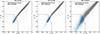 |
Fig. B.1. Comparison between the number of B24A QSO candidates (blue) per magnitude bin in the EDF-N. In grey we show all Euclid compact sources in the corresponding magnitude bin. As the magnitude bins progress from brighter colours (left plot) to fainter (right plot), the number of sources and QSO candidates increases accordingly. |
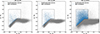 |
Fig. B.3. Comparison between the number of QSO candidates (blue) per magnitude bin in the EDF-N for the new Euclid-only colour cut, JH_IEY. In grey we show all Euclid compact sources in the corresponding magnitude bin. As the magnitude bins progress from brighter colours (left plot) to fainter (right plot), the number of sources and QSO candidates increases accordingly. |
Appendix C: Comparison between AGN selections
We present the intersection table for the different selection methods investigated in this work, excluding the morphology-based methods from SG25 and MB25 due to their distinct methodologies (see fig. 13). We limit the depth of every selection to IE < 22 to ensure comparability without bias towards the Euclid-based selections, which are the only ones capable of reaching the faintest magnitudes.
EDF-N intersection matrix between the different AGN selection methods investigated in this work, excluding the morphology based ones, and limited to 18 < IE ≤ 22.
EDF-S intersection matrix between the different AGN selection methods investigated in this work, excluding the morphology based ones, and limited to 18 < IE ≤ 22.
EDF-F intersection matrix between the different AGN selection methods investigated in this work, excluding the morphology based ones, and limited to 18 < IE ≤ 22.
Appendix D: Column description of AGN catalogues
We list column descriptions for the three EDFs’ catalogues below.
-
objectideuclid: Euclid unique source identifier.
-
raeuclid: Euclid right ascension (J2000.0).
-
deceuclid: Euclid declination (J2000.0).
-
objectidgalex: GALEX source identifier.
-
ragalex: GALEX right ascension (J2000.0).
-
decgalex: GALEX declination (J2000.0).
-
objectidgaia: Gaia unique source identifier.
-
ragaia: Gaia right ascension (ICRS).
-
decgaia: Gaia declination (ICRS).
-
objectiddes: DES unique identifier for the coadded objects. Only available in EDF-S and EDF-F.
-
rades: DES right ascension (J2000.0). Only available in EDF-S and EDF-F.
-
decdes: DES declination (J2000.0). Only available in EDF-S and EDF-F.
-
objectidallwise: WISE-AllWISE unique source identifier.
-
raallwise: WISE-AllWISE right ascension (J2000.0).
-
decallwise: WISE-AllWISE declination (J2000.0)
-
objectiddesi: DESI unique target ID. Only available in EDF-N.
-
radesi: DESI right ascension (ICRS). Only available in EDF-N.
-
decdesi: DESI declination (ICRS). Only available in EDF-N. Only available in EDF-N.
-
Zdesi: DESI redshift measured by Redrock. Only available in EDF-N.
-
objectidsdss: SDSS object identification number. Only available in EDF-N.
-
rasdss: SDSS right ascension (J2000.0). Only available in EDF-N.
-
decsdss: SDSS declination (J2000.0). Only available in EDF-N.
-
Zsdss: SDSS best available redshift. Only available in EDF-N.
-
goodflags: cleaning implemented to keep only those sources with ‘good flags’.
-
brightvismagbin: bright IE magnitude bin: 18 < IE ≤ 21.
-
mediumvismagbin: medium IE magnitude bin: 21 < IE ≤ 22.
-
faintvismagbin: faint IE magnitude bin: 22 < IE ≤ 24.5.
-
starcandidategaia: stellar candidate based on Gaia’s proper motion and parallax.
-
starcandidatePRF: stellar candidate based on PRF star probability > 0.7.
-
starcandidateall: stellar candidate based on starcandidategaia and/or starcandidatePRF.
-
PRFqsocandidate: QSO candidate based on PRF QSO probability> 0.85 in the EDF-N and > 0.95 in the EDF-S and EDF-F.
-
B24aqsocandidate: QSO candidate based on B24A.
-
B24bqsocandidate: QSO candidate based on B24B. Only available in EDF-N.
-
C75agncandidate: AGN candidate based on C75.
-
R90agncandidate: AGN candidate based on R90.
-
GDR3qsocandidate: QSO candidate based on GDR3-QSO.
-
JHIeYqsocandidate: QSO candidate based on JH_IEY.
-
IeHgzqsocandidate: QSO candidate based on IEH_gz.
-
DESIqsocandidate: QSO candidate based on DESI SPECTYPE==QSO.
-
DESIbroadlinegalaxycandidate: AGN candidate based on DESI SPECTYPE==GALAXY and presence of broad emission lines. Only available in EDF-N.
-
DESIbroadlineqsocandidate: QSO candidate based on DESI SPECTYPE==QSO and presence of broad emission lines. Only available in EDF-N.
-
DESIniibptagncandidate: AGN candidate based on DESI SPECTYPE==GALAXY and N II BPT diagnostic. Only available in EDF-N.
-
DESIsiibptagncandidate: AGN candidate based on DESI SPECTYPE==GALAXY and S II BPT diagnostic. Only available in EDF-N.
-
DESIoibptagncandidate: AGN candidate based on DESI SPECTYPE==GALAXY and O I BPT diagnostic. Only available in EDF-N.
-
DESIwhanagncandidate: AGN candidate based on DESI SPECTYPE==GALAXY and WHAN diagnostic. Only available in EDF-N.
-
DESIblueagncandidate: AGN candidate based on DESI SPECTYPE==GALAXY and Blue diagnostic. Only available in EDF-N.
-
DESIkexagncandidate: AGN candidate based on DESI SPECTYPE==GALAXY and KEX diagnostic. Only available in EDF-N.
-
AGNfraction: AGN fraction derived from SED fitting. Only available in EDF-N.
-
AGNfractionerr: AGN fraction error derived from SED fitting. Only available in EDF-N.
-
AGNsedcandidate: AGN candidate based on AGN fraction > 0.25. Only available in EDF-N.
All Tables
Right ascension and declination of each EDF from Euclid Collaboration: Aussel et al. (2026) and their respective number of sources and impact of quality cuts.
EDF-N intersection matrix between the different AGN selection methods investigated in this work, excluding the morphology based ones, and limited to 18 < IE ≤ 22.
EDF-S intersection matrix between the different AGN selection methods investigated in this work, excluding the morphology based ones, and limited to 18 < IE ≤ 22.
EDF-F intersection matrix between the different AGN selection methods investigated in this work, excluding the morphology based ones, and limited to 18 < IE ≤ 22.
All Figures
|
Fig. 1. Sketch outlining the steps adopted in this work to attain the AGN candidate catalogues. We report the number of stellar and AGN candidates for the magnitude range 18 < IE ≤ 24.5. |
| In the text | |
|
Fig. 2. Parameter of MUMAX_MINUS_MAG versus IE for sources in the EDF-N. The colour scale indicates the point like probability of a source. The dotted line indicates the threshold (MUMAX_MINUS_MAG < −2.6) below which most sources appear to be point-like. |
| In the text | |
|
Fig. 3. Selection criteria of B24A applied to the EDF-N. In grey we show all quality-filtered Euclid compact sources, while the QSO candidates are shown in blue. We also showcase, with the black dotted line, the limit of the B24A selection. |
| In the text | |
|
Fig. 4. Selection criteria of B24B applied to the EDF-N. In grey we show all quality-filtered Euclid point-like sources, while the QSO candidates are shown in blue. We also showcase, with the black dotted line, the limit of the B24B selection. |
| In the text | |
|
Fig. 5. WISE-AllWISE AGN candidates in the EDF-N defined by Eq. (4) (top panel) and Eq. (5) (bottom panel). In grey we show all Euclid sources with WISE-AllWISE counterparts, while the blue sources represent the selected AGN candidates. The black dotted lines represent the limits of the C75 and R90 selections. The stellar candidates have already been removed from the samples of AGN candidates. |
| In the text | |
|
Fig. 6. New colour-cut criteria (black dotted line) defined by Eq. (6) applied to EDF-N. In grey we show all Euclid compact sources that have a DESI counterpart. The blue coloured points represent the Euclid compact sources selected as DESI BLQSO candidates and the red ones represent the Euclid compact objects selected as galaxy candidates by DESI. Moreover, the purple lines represent the 68% (solid) and 95% (dashed) contours of the stellar candidates found in Sect. 3.1. |
| In the text | |
|
Fig. 7. New colour-cut criteria (black dotted line) defined by Eq. (7) applied to EDF-N. In grey we show all Euclid compact sources with that contained a DESI counterpart. The blue coloured points represent the Euclid compact sources selected as DESI BLQSO candidates and the red ones represent the Euclid compact objects selected as galaxy candidates by DESI. Moreover, the purple lines represent the 68% (solid) and 95% (dashed) contours of the stellar candidates found in Sect. 3.1. |
| In the text | |
|
Fig. 8. Emission line diagnostic diagram of N II (left), S II (centre), and O I (right) for the Euclid sources with a DESI spectroscopic counterpart. |
| In the text | |
|
Fig. 9. Normalised cumulative distribution of the AGN fraction measured by SED fitting for the different AGN selection methods in EDFN: C75/R90 (green solid/purple dashed), B24A/B (grey/lime dashed), spectroscopically confirmed broad-line or narrow-line AGN (red dash-dotted/cyan solid), IEH_gz (yellow solid), JH_IEY (black dash-dotted), PRF (dark blue dotted, TM25), and X-ray (pink solid,, RW25). The blue dashed-dotted line is the inverse cumulative distribution of all non-AGN candidates. The vertical black solid line represents the proposed AGN fraction threshold (fAGN = 0.25) discriminating AGN and non-AGN sources, while the horizontal black dotted line shows the corresponding false-positive probability (23%). We note that only two X-ray sources have counterparts with zspec in the quality-filtered EDF-N catalogue. |
| In the text | |
|
Fig. 10. Comparison of AGN surface densities obtained from the selection methods discussed in this work divided into energy bands: X-ray selections (blue), optical selections (shades of green), and IR selections (shades of orange). For the selections B24A, B24B, JH_IEY, IEH_gz, C75, R90, DESI, and PRF, the AGN surface densities are split into 18 < IE ≤ 24.5 (upside down triangles) and 18 < IE ≤ 22 (upside up triangles). For the GDR3-QSOs, only the 18 < IE ≤ 22 is shown due to the limiting magnitude of Gaia. Individual markers indicate AGN surface densities from other Q1 related works, including X-ray candidates from RW25 (with the lower limit indicated by an arrow pointing up); diffusion model candidates from SG25 (plus sign); deep learning candidates from MB25 (cross); and AGN fraction candidates from from LB25 (hexagon). The predictions for the detectable AGN (purple horizontal solid line) and identifiable AGN (purple dashed line) in the EWS from SM25 are included. The grey horizontal dashed line represents recovered AGN surface density by eFEDS (Liu et al. 2022a). |
| In the text | |
|
Fig. 11. Selection JH versus IEY (black dotted line) applied to the EDF-N. In grey we show all Euclid compact sources. The red coloured dots represent the X-ray selected AGN candidates from RW25, while the purple dots indicate the GDR3-QSOs, which mainly lie within the selection. |
| In the text | |
|
Fig. 12. Selection IEH versus gz (black dotted line) applied to the EDF-N. In grey we show all Euclid compact sources. The red coloured dots represent the X-ray selected AGN candidates from RW25, while the purple dots indicate the GDR3-QSOs, which mainly lie within the selection. |
| In the text | |
|
Fig. 13. Comparison among the number of sources selected as AGN candidates for the different criteria investigated in this work per EDF. We exclude the morphology-based AGN candidates from SG25 and MB25 due to the significant differences in their methodologies compared to other techniques explored in this work. X-ray candidates correspond to those sources from RW25 and PRF correspond to the purified sample from TM25. We set the detection limit to the range of 18 < IE ≤ 22, ensuring all selections match in depth. We note that EDF-N shows more selection criteria than EDF-S and EDF-F due to the available u-band photometry from UNIONS and spectroscopy from DESI in the EDF-N. |
| In the text | |
|
Fig. 14. Selection IEH versus gz (black dotted line) applied to the EDF-N. In grey we show all Euclid sources. The blue dots represent the N II selected AGN candidates, the composite galaxies are shown in purple, the SFGs in red and the LINERs in green. |
| In the text | |
|
Fig. 15. Spectral energy distributions and corresponding VIS cutouts of two QSO candidates identified by the selections JH_IEY, IEH_gz, B24A, B24B and simultaneously classified as broad-line QSOs by DESI. |
| In the text | |
|
Fig. 16. Spectral energy distributions and corresponding VIS cutouts of two narrow-line AGN candidates identified via BPT diagnostics. |
| In the text | |
|
Fig. B.1. Comparison between the number of B24A QSO candidates (blue) per magnitude bin in the EDF-N. In grey we show all Euclid compact sources in the corresponding magnitude bin. As the magnitude bins progress from brighter colours (left plot) to fainter (right plot), the number of sources and QSO candidates increases accordingly. |
| In the text | |
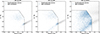 |
Fig. B.2. The same as Fig. B.1, but for B24B |
| In the text | |
|
Fig. B.3. Comparison between the number of QSO candidates (blue) per magnitude bin in the EDF-N for the new Euclid-only colour cut, JH_IEY. In grey we show all Euclid compact sources in the corresponding magnitude bin. As the magnitude bins progress from brighter colours (left plot) to fainter (right plot), the number of sources and QSO candidates increases accordingly. |
| In the text | |
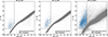 |
Fig. B.4. Same as B.3 but for IEH_gz. |
| In the text | |
Current usage metrics show cumulative count of Article Views (full-text article views including HTML views, PDF and ePub downloads, according to the available data) and Abstracts Views on Vision4Press platform.
Data correspond to usage on the plateform after 2015. The current usage metrics is available 48-96 hours after online publication and is updated daily on week days.
Initial download of the metrics may take a while.