


| Issue |
A&A
Volume 711, July 2026
Euclid Quick Data Release (Q1)
|
|
|---|---|---|
| Article Number | A18 | |
| Number of page(s) | 21 | |
| Section | Extragalactic astronomy | |
| DOI | https://doi.org/10.1051/0004-6361/202554583 | |
| Published online | 30 June 2026 | |
Euclid Quick Data Release (Q1)
XVIII. First Euclid statistical study of the active galactic nuclei contribution fraction
1
SRON Netherlands Institute for Space Research, Landleven 12, 9747, AD, Groningen, The Netherlands
2
Kapteyn Astronomical Institute, University of Groningen, PO Box 800, 9700 AV, Groningen, The Netherlands
3
Instituto de Radioastronomía y Astrofísica, Universidad Nacional Autónoma de México, A.P. 72-3, 58089 Morelia, Mexico
4
Instituto de Astrofísica e Ciências do Espaço, Universidade do Porto, CAUP, Rua das Estrelas, PT4150-762 Porto, Portugal
5
DTx – Digital Transformation CoLAB, Building 1, Azurém Campus, University of Minho, 4800-058 Guimarães, Portugal
6
School of Physics, HH Wills Physics Laboratory, University of Bristol, Tyndall Avenue, Bristol BS8 1TL, UK
7
Department of Mathematics and Physics, Roma Tre University, Via della Vasca Navale 84, 00146 Rome, Italy
8
INAF-Osservatorio Astronomico di Roma, Via Frascati 33, 00078 Monteporzio Catone, Italy
9
Department of Physical Sciences, Ritsumeikan University, Kusatsu, Shiga 525-8577, Japan
10
National Astronomical Observatory of Japan, 2-21-1 Osawa, Mitaka, Tokyo 181-8588, Japan
11
Academia Sinica Institute of Astronomy and Astrophysics (ASIAA), 11F of ASMAB, No. 1, Section 4, Roosevelt Road, Taipei 10617, Taiwan
12
Institute of Space Sciences (ICE, CSIC), Campus UAB, Carrer de Can Magrans, s/n, 08193 Barcelona, Spain
13
Institut d’Estudis Espacials de Catalunya (IEEC), Edifici RDIT, Campus UPC, 08860 Castelldefels, Barcelona, Spain
14
Max Planck Institute for Extraterrestrial Physics, Giessenbachstr. 1, 85748 Garching, Germany
15
Instituto de Astrofísica de Canarias, Vía Láctea, 38205 La Laguna, Tenerife, Spain
16
Universidad de La Laguna, Departamento de Astrofísica, 38206 La Laguna, Tenerife, Spain
17
Instituto de Astrofísica de Canarias (IAC); Departamento de Astrofísica, Universidad de La Laguna (ULL), 38200 La Laguna, Tenerife, Spain
18
School of Physics & Astronomy, University of Southampton, Highfield Campus, Southampton SO17 1BJ, UK
19
INAF-Istituto di Astrofisica e Planetologia Spaziali, Via del Fosso del Cavaliere, 100, 00100 Roma, Italy
20
Leiden Observatory, Leiden University, Einsteinweg 55, 2333 CC, Leiden, The Netherlands
21
Institute for Astronomy, University of Edinburgh, Royal Observatory, Blackford Hill, Edinburgh EH9 3HJ, UK
22
Université Paris-Saclay, CNRS, Institut d’astrophysique spatiale, 91405 Orsay, France
23
ESAC/ESA, Camino Bajo del Castillo, s/n., Urb. Villafranca del Castillo, 28692 Villanueva de la Cañada, Madrid, Spain
24
School of Mathematics and Physics, University of Surrey, Guildford, Surrey GU2 7XH, UK
25
INAF-Osservatorio Astronomico di Brera, Via Brera 28, 20122 Milano, Italy
26
INAF-Osservatorio di Astrofisica e Scienza dello Spazio di Bologna, Via Piero Gobetti 93/3, 40129 Bologna, Italy
27
Université Paris-Saclay, Université Paris Cité, CEA, CNRS, AIM, 91191 Gif-sur-Yvette, France
28
IFPU, Institute for Fundamental Physics of the Universe, Via Beirut 2, 34151 Trieste, Italy
29
INAF-Osservatorio Astronomico di Trieste, Via G. B. Tiepolo 11, 34143 Trieste, Italy
30
INFN, Sezione di Trieste, Via Valerio 2, 34127 Trieste TS, Italy
31
SISSA, International School for Advanced Studies, Via Bonomea 265, 34136 Trieste, TS, Italy
32
Dipartimento di Fisica e Astronomia, Università di Bologna, Via Gobetti 93/2, 40129 Bologna, Italy
33
INFN-Sezione di Bologna, Viale Berti Pichat 6/2, 40127 Bologna, Italy
34
INAF-Osservatorio Astronomico di Padova, Via dell’Osservatorio 5, 35122 Padova, Italy
35
Space Science Data Center, Italian Space Agency, Via del Politecnico snc, 00133 Roma, Italy
36
INAF-Osservatorio Astrofisico di Torino, Via Osservatorio 20, 10025 Pino Torinese, (TO), Italy
37
Dipartimento di Fisica, Università di Genova, Via Dodecaneso 33, 16146 Genova, Italy
38
INFN-Sezione di Genova, Via Dodecaneso 33, 16146 Genova, Italy
39
Department of Physics “E. Pancini”, University Federico II, Via Cinthia 6, 80126 Napoli, Italy
40
INAF-Osservatorio Astronomico di Capodimonte, Via Moiariello 16, 80131 Napoli, Italy
41
Faculdade de Ciências da Universidade do Porto, Rua do Campo de Alegre, 4150-007 Porto, Portugal
42
Dipartimento di Fisica, Università degli Studi di Torino, Via P. Giuria 1, 10125 Torino, Italy
43
INFN-Sezione di Torino, Via P. Giuria 1, 10125 Torino, Italy
44
European Space Agency/ESTEC, Keplerlaan 1, 2201 AZ, Noordwijk, The Netherlands
45
Institute Lorentz, Leiden University, Niels Bohrweg 2, 2333, CA, Leiden, The Netherlands
46
INAF-IASF Milano, Via Alfonso Corti 12, 20133 Milano, Italy
47
Centro de Investigaciones Energéticas, Medioambientales y Tecnológicas (CIEMAT), Avenida Complutense 40, 28040 Madrid, Spain
48
Port d’Informació Científica, Campus UAB, C. Albareda s/n, 08193 Bellaterra (Barcelona), Spain
49
Institute for Theoretical Particle Physics and Cosmology (TTK), RWTH Aachen University, 52056 Aachen, Germany
50
INFN section of Naples, Via Cinthia 6, 80126 Napoli, Italy
51
Institute for Astronomy, University of Hawaii, 2680 Woodlawn Drive, Honolulu, HI 96822, USA
52
Dipartimento di Fisica e Astronomia “Augusto Righi” – Alma Mater Studiorum Università di Bologna, Viale Berti Pichat 6/2, 40127 Bologna, Italy
53
Jodrell Bank Centre for Astrophysics, Department of Physics and Astronomy, University of Manchester, Oxford Road, Manchester M13 9PL, UK
54
European Space Agency/ESRIN, Largo Galileo Galilei 1, 00044 Frascati, Roma, Italy
55
Université Claude Bernard Lyon 1, CNRS/IN2P3, IP2I Lyon, UMR 5822, Villeurbanne F-69100, France
56
Aix-Marseille Université, CNRS, CNES, LAM, Marseille, France
57
Institut de Ciències del Cosmos (ICCUB), Universitat de Barcelona (IEEC-UB), Martí i Franquès 1, 08028 Barcelona, Spain
58
Institució Catalana de Recerca i Estudis Avançats (ICREA), Passeig de Lluís Companys 23, 08010 Barcelona, Spain
59
UCB Lyon 1, CNRS/IN2P3, IUF, IP2I Lyon, 4 rue Enrico Fermi, 69622 Villeurbanne, France
60
Mullard Space Science Laboratory, University College London, Holmbury St Mary, Dorking, Surrey RH5 6NT, UK
61
Departamento de Física, Faculdade de Ciências, Universidade de Lisboa, Edifício C8, Campo Grande, PT1749-016 Lisboa, Portugal
62
Instituto de Astrofísica e Ciências do Espaço, Faculdade de Ciências, Universidade de Lisboa, Campo Grande, 1749-016 Lisboa, Portugal
63
Department of Astronomy, University of Geneva, ch. d’Ecogia 16, 1290 Versoix, Switzerland
64
Aix-Marseille Université, CNRS/IN2P3, CPPM, Marseille, France
65
INFN-Bologna, Via Irnerio 46, 40126 Bologna, Italy
66
Universitäts-Sternwarte München, Fakultät für Physik, Ludwig-Maximilians-Universität München, Scheinerstrasse 1, 81679 München, Germany
67
FRACTAL S.L.N.E., calle Tulipán 2, Portal 13 1A, 28231 Las Rozas de Madrid, Spain
68
Dipartimento di Fisica “Aldo Pontremoli”, Università degli Studi di Milano, Via Celoria 16, 20133 Milano, Italy
69
INFN-Sezione di Milano, Via Celoria 16, 20133 Milano, Italy
70
NRC Herzberg, 5071 West Saanich Rd, Victoria, BC V9E 2E7, Canada
71
Institute of Theoretical Astrophysics, University of Oslo, P.O. Box 1029 Blindern 0315, Oslo, Norway
72
Jet Propulsion Laboratory, California Institute of Technology, 4800 Oak Grove Drive, Pasadena, CA 91109, USA
73
Department of Physics, Lancaster University, Lancaster LA1 4YB, UK
74
Felix Hormuth Engineering, Goethestr. 17, 69181 Leimen, Germany
75
Technical University of Denmark, Elektrovej 327, 2800 Kgs., Lyngby, Denmark
76
Cosmic Dawn Center (DAWN), Denmark
77
Institut d’Astrophysique de Paris, UMR 7095, CNRS, and Sorbonne Université, 98 bis boulevard Arago, 75014 Paris, France
78
Max-Planck-Institut für Astronomie, Königstuhl 17, 69117 Heidelberg, Germany
79
NASA Goddard Space Flight Center, Greenbelt, MD 20771, USA
80
Department of Physics and Helsinki Institute of Physics, Gustaf Hällströmin katu 2, 00014 University of Helsinki, Finland
81
Université de Genève, Département de Physique Théorique and Centre for Astroparticle Physics, 24 quai Ernest-Ansermet, CH-1211 Genève 4, Switzerland
82
Department of Physics, P.O. Box 64, 00014 University of Helsinki, Finland
83
Helsinki Institute of Physics, Gustaf Hällströmin katu 2, University of Helsinki, Helsinki, Finland
84
Centre de Calcul de l’IN2P3/CNRS, 21 avenue Pierre de Coubertin, 69627 Villeurbanne Cedex, France
85
Laboratoire d’etude de l’Univers et des phenomenes eXtremes, Observatoire de Paris, Université PSL, Sorbonne Université, CNRS, 92190 Meudon, France
86
SKA Observatory, Jodrell Bank, Lower Withington, Macclesfield, Cheshire SK11 9FT, UK
87
University of Applied Sciences and Arts of Northwestern Switzerland, School of Computer Science, 5210 Windisch, Switzerland
88
Universität Bonn, Argelander-Institut für Astronomie, Auf dem Hügel 71, 53121 Bonn, Germany
89
INFN-Sezione di Roma, Piazzale Aldo Moro, 2 – c/o Dipartimento di Fisica, Edificio G. Marconi, 00185 Roma, Italy
90
Dipartimento di Fisica e Astronomia “Augusto Righi” – Alma Mater Studiorum Università di Bologna, Via Piero Gobetti 93/2, 40129 Bologna, Italy
91
Department of Physics, Institute for Computational Cosmology, Durham University, South Road, Durham DH1 3LE, UK
92
Université Côte d’Azur, Observatoire de la Côte d’Azur, CNRS, Laboratoire Lagrange, Bd de l’Observatoire, CS 34229, 06304 Nice cedex 4, France
93
Université Paris Cité, CNRS, Astroparticule et Cosmologie, 75013 Paris, France
94
CNRS-UCB International Research Laboratory, Centre Pierre Binetruy, IRL2007, CPB-IN2P3 Berkeley, USA
95
University of Applied Sciences and Arts of Northwestern Switzerland, School of Engineering, 5210 Windisch, Switzerland
96
Institut d’Astrophysique de Paris, 98bis Boulevard Arago, 75014 Paris, France
97
Institute of Physics, Laboratory of Astrophysics, Ecole Polytechnique Fédérale de Lausanne (EPFL), Observatoire de Sauverny, 1290 Versoix, Switzerland
98
Aurora Technology for European Space Agency (ESA), Camino bajo del Castillo, s/n, Urbanizacion Villafranca del Castillo, Villanueva de la Cañada, 28692 Madrid, Spain
99
Institut de Física d’Altes Energies (IFAE), The Barcelona Institute of Science and Technology, Campus UAB, 08193 Bellaterra (Barcelona), Spain
100
School of Mathematics, Statistics and Physics, Newcastle University, Herschel Building, Newcastle-upon-Tyne, NE1 7RU, UK
101
DARK, Niels Bohr Institute, University of Copenhagen, Jagtvej 155, 2200 Copenhagen, Denmark
102
Waterloo Centre for Astrophysics, University of Waterloo, Waterloo, Ontario N2L 3G1, Canada
103
Department of Physics and Astronomy, University of Waterloo, Waterloo, Ontario N2L 3G1, Canada
104
Perimeter Institute for Theoretical Physics, Waterloo, Ontario N2L 2Y5, Canada
105
Centre National d’Etudes Spatiales – Centre spatial de Toulouse, 18 avenue Edouard Belin, 31401 Toulouse Cedex 9, France
106
Institute of Space Science, Str. Atomistilor, nr. 409 Măgurele, Ilfov 077125, Romania
107
Consejo Superior de Investigaciones Cientificas, Calle Serrano 117, 28006 Madrid, Spain
108
Dipartimento di Fisica e Astronomia “G. Galilei”, UniversitUniversità di Padova, Via Marzolo 8, 35131 Padova, Italy
109
INFN-Padova, Via Marzolo 8, 35131 Padova, Italy
110
Caltech/IPAC, 1200 E. California Blvd., Pasadena, CA 91125, USA
111
Institut für Theoretische Physik, University of Heidelberg, Philosophenweg 16, 69120 Heidelberg, Germany
112
Institut de Recherche en Astrophysique et Planétologie (IRAP), Université de Toulouse, CNRS, UPS, CNES, 14 Av. Edouard Belin, 31400 Toulouse, France
113
Université St Joseph; Faculty of Sciences, Beirut, Lebanon
114
Departamento de Física, FCFM, Universidad de Chile, Blanco Encalada, 2008 Santiago, Chile
115
Universität Innsbruck, Institut für Astro- und Teilchenphysik, Technikerstr. 25/8, 6020 Innsbruck, Austria
116
Satlantis, University Science Park, Sede Bld 48940, Leioa-Bilbao, Spain
117
Instituto de Astrofísica e Ciências do Espaço, Faculdade de Ciências, Universidade de Lisboa, Tapada da Ajuda, 1349-018 Lisboa, Portugal
118
Cosmic Dawn Center (DAWN)
119
Niels Bohr Institute, University of Copenhagen, Jagtvej 128, 2200 Copenhagen, Denmark
120
Universidad Politécnica de Cartagena, Departamento de Electrónica y Tecnología de Computadoras, Plaza del Hospital 1, 30202 Cartagena, Spain
121
Infrared Processing and Analysis Center, California Institute of Technology, Pasadena, CA 91125, USA
122
Dipartimento di Fisica e Scienze della Terra, Università degli Studi di Ferrara, Via Giuseppe Saragat 1, 44122 Ferrara, Italy
123
Istituto Nazionale di Fisica Nucleare, Sezione di Ferrara, Via Giuseppe Saragat 1, 44122 Ferrara, Italy
124
INAF, Istituto di Radioastronomia, Via Piero Gobetti 101, 40129 Bologna, Italy
125
Department of Physics, Oxford University, Keble Road, Oxford OX1 3RH, UK
126
Université PSL, Observatoire de Paris, Sorbonne Université, CNRS, LERMA, 75014 Paris, France
127
Université Paris-Cité, 5 Rue Thomas Mann, 75013, Paris, France
128
INAF – Osservatorio Astronomico di Brera, Via Emilio Bianchi 46, 23807 Merate, Italy
129
INAF-Osservatorio Astronomico di Brera, Via Brera 28, 20122, Milano, Italy and INFN-Sezione di Genova, Via Dodecaneso 33, 16146 Genova, Italy
130
ICL, Junia, Université Catholique de Lille, LITL, 59000 Lille, France
131
ICSC – Centro Nazionale di Ricerca in High Performance Computing, Big Data e Quantum Computing, Via Magnanelli 2, Bologna, Italy
132
Instituto de Física Teórica UAM-CSIC, Campus de Cantoblanco, 28049 Madrid, Spain
133
CERCA/ISO, Department of Physics, Case Western Reserve University, 10900 Euclid Avenue, Cleveland, OH 44106, USA
134
Technical University of Munich, TUM School of Natural Sciences, Physics Department, James-Franck-Str. 1, 85748 Garching, Germany
135
Max-Planck-Institut für Astrophysik, Karl-Schwarzschild-Str. 1, 85748 Garching, Germany
136
Laboratoire Univers et Théorie, Observatoire de Paris, Université PSL, Université Paris Cité, CNRS, 92190 Meudon, France
137
Departamento de Física Fundamental. Universidad de Salamanca., Plaza de la Merced s/n., 37008 Salamanca, Spain
138
Université de Strasbourg, CNRS, Observatoire astronomique de Strasbourg, UMR 7550, 67000 Strasbourg, France
139
Center for Data-Driven Discovery, Kavli IPMU (WPI), UTIAS, The University of Tokyo, Kashiwa, Chiba 277-8583, Japan
140
Ludwig-Maximilians-University, Schellingstrasse 4, 80799 Munich, Germany
141
Max-Planck-Institut für Physik, Boltzmannstr. 8, 85748 Garching, Germany
142
Dipartimento di Fisica – Sezione di Astronomia, Università di Trieste, Via Tiepolo 11, 34131 Trieste, Italy
143
California Institute of Technology, 1200 E California Blvd, Pasadena, CA 91125, USA
144
Department of Physics & Astronomy, University of California Irvine, Irvine, CA 92697, USA
145
Department of Mathematics and Physics E. De Giorgi, University of Salento, Via per Arnesano, CP-I93, 73100 Lecce, Italy
146
INFN, Sezione di Lecce, Via per Arnesano, CP-193, 73100 Lecce, Italy
147
INAF-Sezione di Lecce, c/o Dipartimento Matematica e Fisica, Via per Arnesano, 73100 Lecce, Italy
148
Departamento Física Aplicada, Universidad Politécnica de Cartagena, Campus Muralla del Mar, 30202 Cartagena, Murcia, Spain
149
Instituto de Física de Cantabria, Edificio Juan Jordá, Avenida de los Castros, 39005 Santander, Spain
150
CEA Saclay, DFR/IRFU, Service d’Astrophysique, Bat. 709, 91191 Gif-sur-Yvette, France
151
Institute of Cosmology and Gravitation, University of Portsmouth, Portsmouth PO1 3FX, UK
152
Department of Computer Science, Aalto University, PO Box 15400 Espoo FI-00 076, Finland
153
Instituto de Astrofísica de Canarias, c/ Via Lactea s/n, La Laguna, 38200, Spain. Departamento de Astrofísica de la Universidad de La Laguna, Avda. Francisco Sanchez, La Laguna, 38200, Spain
154
Ruhr University Bochum, Faculty of Physics and Astronomy, Astronomical Institute (AIRUB), German Centre for Cosmological Lensing (GCCL), 44780 Bochum, Germany
155
Department of Physics and Astronomy, Vesilinnantie 5, 20014 University of Turku, Finland
156
Serco for European Space Agency (ESA), Camino bajo del Castillo, s/n, Urbanizacion Villafranca del Castillo, Villanueva de la Cañada, 28692, Madrid, Spain
157
ARC Centre of Excellence for Dark Matter Particle Physics, Melbourne, Australia
158
Centre for Astrophysics & Supercomputing, Swinburne University of Technology, Hawthorn, Victoria 3122, Australia
159
Department of Physics and Astronomy, University of the Western Cape, Bellville, Cape Town, 7535, South Africa
160
DAMTP, Centre for Mathematical Sciences, Wilberforce Road, Cambridge CB3 0WA, UK
161
Kavli Institute for Cosmology Cambridge, Madingley Road, Cambridge CB3 0HA, UK
162
Department of Astrophysics, University of Zurich, Winterthurerstrasse 190, 8057 Zurich, Switzerland
163
Department of Physics, Centre for Extragalactic Astronomy, Durham University, South Road, Durham DH1 3LE, UK
164
IRFU, CEA, Université Paris-Saclay, 91191 Gif-sur-Yvette Cedex, France
165
Oskar Klein Centre for Cosmoparticle Physics, Department of Physics, Stockholm University, Stockholm SE-106 91, Sweden
166
Astrophysics Group, Blackett Laboratory, Imperial College London, London SW7 2AZ, UK
167
Univ. Grenoble Alpes, CNRS, Grenoble INP, LPSC-IN2P3, 53, Avenue des Martyrs, 38000 Grenoble, France
168
INAF-Osservatorio Astrofisico di Arcetri, Largo E. Fermi 5, 50125 Firenze, Italy
169
Dipartimento di Fisica, Sapienza Università di Roma, Piazzale Aldo Moro 2, 00185 Roma, Italy
170
Centro de Astrofísica da Universidade do Porto, Rua das Estrelas, 4150-762 Porto, Portugal
171
HE Space for European Space Agency (ESA), Camino bajo del Castillo, s/n, Urbanizacion Villafranca del Castillo, Villanueva de la Cañada, 28692, Madrid, Spain
172
Department of Astrophysical Sciences, Peyton Hall, Princeton University, Princeton, NJ 08544, USA
173
Theoretical astrophysics, Department of Physics and Astronomy, Uppsala University, Box 515, 751 20 Uppsala, Sweden
174
Minnesota Institute for Astrophysics, University of Minnesota, 116 Church St SE, Minneapolis, MN 55455, USA
175
Mathematical Institute, University of Leiden, Einsteinweg 55, 2333, CA, Leiden, The Netherlands
176
Institute of Astronomy, University of Cambridge, Madingley Road, Cambridge CB3 0HA, UK
177
Space Physics and Astronomy Research Unit, University of Oulu, Pentti Kaiteran katu 1, FI-90014 Oulu, Finland
178
Center for Computational Astrophysics, Flatiron Institute, 162 5th Avenue, 10010 New York, NY, USA
179
Department of Physics and Astronomy, University of British Columbia, Vancouver, BC V6T 1Z1, Canada
★ Corresponding author: This email address is being protected from spambots. You need JavaScript enabled to view it.
Received:
17
March
2025
Accepted:
20
September
2025
Abstract
Active galactic nuclei (AGN) are an important phase in galaxy evolution. However, they can be difficult to identify due to their varied observational signatures. Furthermore, to understand the impact of an AGN on its host galaxy, it is important to quantify the strength of the AGN with respect to the host galaxy. We developed a deep learning (DL) model to identify AGN in imaging data by deriving the contribution of the central point source. The model was trained with Euclidised mock galaxy images in which we artificially injected different levels of AGN, in the form of varying contributions of the point spread function (PSF). Our DL-based method can precisely and accurately recover the injected AGN contribution fraction, fPSF, with a mean difference between the predicted and true fPSF of −0.0078 and an overall root mean square error of 0.051. With this new method, we move beyond the simplistic AGN versus non-AGN classification and are able to precisely quantify the AGN contribution and study galaxy evolution across a continuous spectrum of AGN activity. We applied our method to a stellar-mass-limited sample (with M* ≥ 109.8 M⊙ and 0.5 ≤ z ≤ 2.0 ) selected from the first Euclid quick data release (Q1) and, using a threshold of fPSF > 0.2, we identified 61 432 ± 70 AGN over 63.1 deg2 (9.8 ± 0.1% of our sample). We compared these DL-selected AGN with AGN selected in the X-ray, mid-infrared (MIR), and via optical spectroscopy and investigated their overlapping fractions depending on different thresholds on the PSF contribution. We find that the overlap increases with increasing X-ray or bolometric AGN luminosity. We observe a positive correlation between the luminosity in the IE filter of the AGN and the host galaxy stellar mass, suggesting that supermassive black holes (SMBHs) generally grow faster (in absolute terms, i.e. the luminosity of the PSF component is larger) in more massive galaxies. Moreover, the mean relative contribution of the AGN is higher in the quiescent galaxy population than in the star-forming population. In terms of absolute power, starburst galaxies, as well as the most massive galaxies (across the star-formation main sequence), tend to host the most luminous AGN, indicating concomitant assembly of the SMBH and the host galaxy.
Key words: galaxies: active / galaxies: statistics
© The Authors 2026
 Open Access article, published by EDP Sciences, under the terms of the Creative Commons Attribution License (https://creativecommons.org/licenses/by/4.0), which permits unrestricted use, distribution, and reproduction in any medium, provided the original work is properly cited.
This article is published in open access under the Subscribe to Open model. This email address is being protected from spambots. You need JavaScript enabled to view it. to support open access publication.
1. Introduction
Active galactic nuclei (AGN) are widely considered to be a crucial phase in the evolution of massive galaxies (Zhuang & Ho 2023), and may also play a role in the growth and regulation of low-mass galaxies (Mezcua et al. 2019; Greene et al. 2020). They are powered by accretion of matter onto the supermassive black holes (SMBHs) at the centres of galaxies and can emit radiation across the whole electromagnetic spectrum (Ueda et al. 2003; Padovani et al. 2017; Bianchi et al. 2022). Active galactic nuclei can be broadly divided into categories, such as type I and type II AGN (Antonucci 1993; Urry & Padovani 1995), depending on their observational characteristics. Type I are unobscured AGN, which are luminous in the ultraviolet and optical. Type II are obscured AGN, in which the dust and gas torus surrounding the central engine can conceal their emission at certain wavelengths. Therefore, they need to be selected using different methods (Hickox & Alexander 2018), such as X-ray luminosity or colour criteria. While methods based on optical colours are affected by dust obscuration, and therefore will be biased against dust-obscured sources, methods based on mid-infrared (MIR) colours will tend to select dust-obscured AGN. The AGN selected based on X-ray emission can include both obscured and unobscured AGN, although the soft X-ray selection tends to be biased towards unobscured sources. However, X-ray selection can be biased towards more massive galaxies (Aird et al. 2012; Mendez et al. 2013; Azadi et al. 2017), as AGN with lower relative accretion rates are more easily detected in such hosts. This bias is not unique to X-ray selection but is a common feature of all flux-limited AGN selection methods.
There exists a close connection between the assembly of the SMBH and the formation and evolution of its host galaxy (Kormendy & Ho 2013). This is seen by various scaling relations between galaxy physical properties (such as stellar velocity dispersion, bulge luminosity, and bulge mass) and the mass of the SMBH (Gültekin et al. 2009; Beifiori et al. 2012; Graham & Scott 2013; McConnell & Ma 2013; Läsker et al. 2014; Shankar et al. 2016). To better measure these correlations and trace their evolution over time, there is clearly a need to accurately separate the light contribution from the accreting SMBH and its host galaxy. Traditionally, one way to achieve this is by performing a two-dimensional (2D) decomposition of the observed surface brightness, in a way that the galaxy is often modelled by a parameterised model, typically a Sérsic profile (Li et al. 2021; Toba et al. 2022), while the AGN component can be assumed to be a point source described by the point spread function (PSF) of the relevant observational instrument. This method can be further customised with different profiles to describe more complex light distributions of the host galaxy and different PSF models to account for any temporal and spatial variations. However, in addition to making simplified assumptions regarding galaxy morphology and structure (which may be particularly problematic for certain galaxy types), the surface brightness fitting approach is very time-consuming, making it unfeasible for large surveys. These fitting methods, based on surface brightness fitting by codes such as GALFIT (Peng et al. 2002), often fail when the galaxy cannot be easily described by a parameterised profile, which can be the case for highly irregular galaxies or merging galaxies, leading to a high failure rate (Ribeiro et al. 2016; Ghosh et al. 2023; Margalef-Bentabol et al. 2026). Another practical difficulty is that traditional methods usually do not have a built-in mechanism to easily take into account systematic effects such as variations in the PSF, which can fundamentally limit the level of precision in the decomposition.
With the advent of the Euclid space telescope (Laureijs et al. 2011) and its uniquely transformative power in high spatial resolution, sensitivity, and survey volume, we have an unprecedented opportunity to trace the co-evolution of the SMBHs and their host galaxies in statistically large samples across cosmic history. However, as was explained above, traditional methods increasingly struggle to cope with the data complexity and volume and often fail to meet the higher requirements on precision and accuracy. To overcome these issues, in this work we use a deep learning (DL) -based method developed in Margalef-Bentabol et al. (2026) to determine the AGN contribution fraction to the total observed light of a galaxy in imaging data. Specifically, we train a DL model with realistic mock images generated from cosmological hydro-dynamical simulations in which we inject AGN at different levels by adjusting the relative contribution of the PSF. Consequently, the trained model can be used to estimate the fraction of the light originating from a central point source, which we can then interpret as the AGN contribution fraction. This method enables a more nuanced study of AGN, moving beyond a binary classification of AGN presence or absence. Some galaxies, while not classified as AGN by traditional selection methods, may still exhibit AGN activity that influences their host galaxies. By quantifying the AGN contribution fraction, we can better assess the role of AGN across a continuum of activity levels. Moreover, for comparisons with other selection techniques (generally binary selection), such as those based on X-ray luminosity, MIR colours, and optical spectroscopy, we can still apply specific thresholds on the PSF contribution fraction to classify AGN candidates. In this work, we present samples of AGN candidates identified with our method and compare them to these alternative selection approaches.
Due to the relatively short timescale of the AGN activity and its diverse observational signatures, it is often challenging to construct sufficiently large samples of AGN to perform robust statistical and multi-dimensional analyses of the AGN population and co-evolution with the host galaxies. With Euclid’s large survey area this problem can be overcome. Furthermore, Euclid’s high spatial resolution and sensitivity make it the perfect survey to which our DL-based method can be applied to analyse the AGN contribution in imaging data. In this paper, we present the first study of identifying AGN using a DL-based image decomposition technique in the first Quick Data Release of the Euclid mission (Q1, Euclid Quick Release Q1 2025). Throughout the paper, we use the terms PSF contribution and AGN contribution interchangeably.
The paper is organised as follows. In Sect. 2, we first briefly introduce the Euclid imaging data used in this work and the key characteristics. Then we explain our galaxy sample selection and the various AGN-selection methods which are used to compare with our DL-based AGN identification method. In Sect. 3, we describe the Euclid mock observations generated from the cosmological hydrodynamic simulations and how they are used to train our DL model. In Sect. 4, first we show in detail the performance of the trained DL model on the simulated test data, using various metrics. Then we compare AGN identified using our method with AGN selected via other commonly used techniques (e.g. via X-ray detections, MIR colour selections, and optical spectroscopy). Finally, using the AGN identified by our model, we examine the relation between the growth of the SMBHs (as traced by the AGN contribution fraction and AGN luminosity) and their host galaxy properties. In Sect. 5, we present our main conclusions and future directions. Throughout the paper we assume a flat Lambda cold dark matter (ΛCDM) universe with Ωm = 0.3089, ΩΛ = 0.6911, and H0 = 67.74 km s−1 Mpc−1 (Planck Collaboration XIII 2016).
2. Data
In this section, we first briefly describe the Euclid data products used in this paper. Then we explain the selection criteria imposed to construct a stellar-mass-limited galaxy sample. Finally, we present various commonly used AGN-selection methods that will be compared with our AGN identification method.
2.1. Euclid data products
For this work, we exploited the Q1 data. A detailed description of the mission and a summary of the scientific objectives are presented in Euclid Collaboration: Mellier et al. (2025), and a description of the DR can be found in Euclid Collaboration: Aussel et al. (2026), Euclid Collaboration: McCracken et al. (2026), Euclid Collaboration: Polenta et al. (2026), and Euclid Collaboration: Romelli et al. (2026). Q1 covers 63.1 deg2 in total in the Euclid Deep Fields (EDFs): North (EDF-N), South (EDF-S), and Fornax (EDF-F), observed by a single visit with the Visible Camera (VIS) in a single broadband filter, IE (Euclid Collaboration: Cropper et al. 2025), and the Near Infrared Spectrometer and Photometer (NISP) instrument in three bands, YE, JE, and HE (Euclid Collaboration: Jahnke et al. 2025).
We made use of a number of data products from Q1, including imaging data and associated catalogues (Altieri et al., in prep.), photometric measurements, and galaxy physical properties, such as stellar masses and star formation rates (SFRs). For a description of the photometric catalogues, see Euclid Collaboration: Romelli et al. (2026). For a complete description of how photometric redshifts (photo-z) and physical properties are inferred in the Q1 data, see Euclid Collaboration: Tucci et al. (2026). We note that photometric redshifts and physical properties are currently estimated without accounting for AGN contribution. As a result, some findings (especially for sources with significant AGN contributions) may be less reliable. Future analyses should incorporate more refined measurements to improve accuracy. For this work, we used the VIS imaging data due to its high spatial resolution, with a pixel resolution of 0 1 pixel−1 and a depth of 24.7 AB mag (10 σ observed depth), observed in the visible filter IE. For each galaxy in our selected sample (see Sect. 2.2), we made a cut-out of 4″ × 4″ (40 pixels × 40 pixels), with the source at the centre. This size corresponds to a physical size of between 25 kpc × 25 kpc and 35 kpc × 35 kpc in the redshift range 0.5 < z < 2. This redshift range was chosen to ensure similar physical size across cut-outs. Along with the VIS images, we used the empirical VIS PSFs (Euclid Collaboration: Cropper et al. 2025). Each source is accompanied by a PSF and, from all available PSFs, we chose a random sample of approximately 500 000 PSFs distributed within all three EDFs. In Fig. 1 we show the stacked PSFs (a randomly selected sub-sample of 500) and display the mean, standard deviation, and coefficient of variation (i.e. the standard deviation divided by the mean). The typical VIS PSF full width at half maximum (FWHM) is 0
 13, which corresponds to a physical scale of approximately 1 kpc at the median redshift of the sample. The mean coefficient of variation is around 13%. This level of intrinsic variation in the observed PSF will later be compared to the precision of our method in recovering the contribution of the PSF in the VIS imaging data (see Sect. 4.1). It is worth noticing that potential differences in the spectral energy distribution (SED) of stars used to generate the PSFs and those of AGN could lead to variations in the shape and size of the PSF. Further work is needed to investigate how these variations depend on the choice and colours of stars, and to assess their impact on our method.
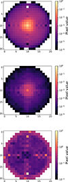 |
Fig. 1. Euclid VIS PSF. We stacked 500 random empirical PSFs and show the mean PSF (top panel), standard deviation (central panel), and the coefficient of variation (bottom panel), calculated pixel by pixel. The pixel resolution is 0 |

2.2. Galaxy sample selection
We constructed our sample of galaxies from the Euclid catalogues by first applying several conditions to remove possible contaminants and ensure a high signal-to-noise (S/N) detection. The conditions applied were the following.
-
VIS_DET = 1 to ensure detection in the IE band.
-
DET_QUALITY_FLAG < 4. This criterion ensured that we removed contaminants in the form of close neighbours, sources blended with another source, saturated sources or sources too close to the border, within the VIS or NIR bright star masks or within an extended source area, and bad pixels.
-
SPURIOUS_FLAG = 0 to remove spurious sources.
-
MUMAX_MINUS_MAG > −2.6 to remove sources that have a high probability of being point-like (Euclid Collaboration: Romelli et al. 2026).
-
IE < 24.5, corresponding to a 10σ detection.
Furthermore, we imposed the following additional criteria to ensure good-quality photo-z (zph) and physical parameter estimations:
-
PHZ_FLAGS = 0;
-
PHYS_PARAM_FLAGS = 0;
-
QUALITY_FLAG = 0.
Finally, we selected galaxies in the redshift range of 0.5 ≤ zph ≤ 2.0 and with stellar mass of M* ≥ 109.8 M⊙. The stellar mass limit chosen here is motivated by Euclid Collaboration: Enia et al. (2026), who, using a similar multi-wavelength sample of galaxies find that at z = 2 and for galaxies with M* ≥ 109.8 M⊙, the sample is more than 90% complete. After all these selection criteria, we are left with a final stellar-mass-limited sample of 624 153 galaxies.
2.3. AGN selections
Active galactic nuclei can exhibit various observational features across the entire electromagnetic spectrum. Consequently, different selection techniques are used to identify different flavours of AGN (e.g. observed with different viewing angles, dust obscuration levels, and/or evolution stages). We used the following three widely used AGN-selection techniques to compare with our DL-based methodology.
X-ray AGN: Galaxies were classified as AGN if they had a counterpart identified in Euclid Collaboration: Roster et al. (2026). Euclid Collaboration: Roster et al. (2026) constructed a catalogue of Q1 galaxies with counterparts in any of the three X-ray surveys that overlap with the EDFs: the XMM-Newton 4XMM-DR14 survey (4XMM; Webb et al. 2020); the Chandra Source Catalog v.2.0 (CSC2; Evans et al. 2024); and the eROSITA DR1 Main sample (EROMAIN; Predehl et al. 2021; Merloni et al. 2024). All three surveys (4XMM, CSC2, and EROMAIN) have a soft X-ray energy range of 0.5–2 keV. However, EROMAIN does not cover EDF-N. The catalogue includes public spectroscopic redshifts (spec-zs), if available. In those cases, we used the spec-z instead of the photo-z from the Q1 catalogue. To select a high-purity sample of X-ray AGN and minimise contaminants, we selected only sources that satisfied the following criteria:
-
match_flag equal to 1, to select sources with the highest individual probability of being the correct counterpart to the X-ray sources, in any of the surveys;
-
a low Galactic probability, Gal_proba < 0.5, to ensure that we selected extragalactic sources;
-
an X-ray signal-to-noise ratio of S/N ≥ 2;
-
a X-ray luminosity of LX [0.5 − 2 keV] ≥ 1042 erg s−1.
There are a total of 335 sources in 4XMM, 14 in CSC2, and 276 in EROMAIN. Figure 2 shows the different sources identified in the LX [0.5 − 2 keV] versus redshift plane. Due to the small number statistics and similar sensitivities, we decided to combine 4XMM and CSC2. At a given redshift, galaxies detected in EROMAIN tend to have higher LX [0.5 − 2 keV]. This is expected given the flux limits of the three X-ray surveys. MIR AGN: The MIR colour-selected AGN selection was done by (Euclid Collaboration: Matamoro Zatarain et al. 2026). They followed the criteria from Assef et al. (2018) to find sources with counterparts in the AllWISE Data Release 6 (DR6, Wright et al. 2010; Mainzer et al. 2011), which integrates data from both the WISE cryogenic and NEOWISE post-cryogenic survey (Mainzer et al. 2011) phases, providing the most complete MIR sky coverage available to date. The AllWISE DR6 mapped the entire sky in the four bands, W1, W2, W3, and W4 (centred at 3.4, 4.6, 12, and 22 μm, respectively), detecting over 747 million sources. Euclid Collaboration: Matamoro Zatarain et al. (2026) used two diagnostics, defined in Assef et al. (2018), to select AGN. The first diagnostic, C75, focusing on achieving 75% completeness for the selected AGN candidates (while achieving 51% reliability), is defined by
 (1)
(1)
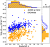 |
Fig. 2. X-ray luminosity of the X-ray-detected Euclid sources as a function of redshift. In blue we show the sources detected in EROMAIN, and in yellow those detected in 4XMM and CSC2. The top histogram shows the redshift distributions of the different samples, and the right histogram shows the distributions in the X-ray luminosity. |
where W1 and W2 are given in the Vega magnitude system. The second diagnostic, R90, focusing on obtaining a sample with 90% reliability (and achieving 17% completeness), is defined as follows:
![Mathematical equation: $$ \begin{aligned} \mathrm W1 - \mathrm W2 > {\left\{ \begin{array}{ll} 0.65 \exp [0.153(\mathrm W2-13.86)^2],&\mathrm {if}\ \mathrm W2>13.86\;,\\ 0.65,&\mathrm {if}\ \mathrm W2 \le 13.86\;.\\ \end{array}\right.} \end{aligned} $$](/articles/aa/full_html/2026/07/aa54583-25/aa54583-25-eq5.gif) (2)
(2)
These two diagnostics must also satisfy the following extra conditions:
-
W1 > 8 and W2 > 7, with S/NW2 ≥ 5, to only consider sources with W1 and W2 magnitudes fainter than the saturation limits of the survey;
-
cc_flags = 0 to ensure that the sources are not artefacts or affected by artefacts (Euclid Collaboration: Matamoro Zatarain et al. 2026).
According to the C75 and R90 diagnostic, there are 9052 and 835 AGN, respectively.
DESI spectroscopic AGN: This AGN selection was done by Euclid Collaboration: Matamoro Zatarain et al. (2026) by selecting the counterparts with the spectroscopically identified AGN in the DESI Early Data Release (DESI Collaboration 2024), with emission line fluxes, widths, and equivalent widths measured with FastSpecFit (Moustakas et al. 2023), including:
-
Quasi-stellar object (QSO) classification based on DESI SPECTYPE (Siudek et al. 2024);
-
AGN classification based on the detection of broad H α, H β, Mg II, or C IV emission lines with a FWHM ≥ 1200 km s−1;
-
AGN classification for DESI sources with a spectroscopic z ≥ 0.5 based on the KEx diagnostic diagram of Zhang & Hao (2018), which makes use of the [O III] λ5007 emission line width, the BLUE diagram of Lamareille (2010), which makes use of the equivalent width of the H β and [O II] λ3727 emission lines, or the WHAN diagram of (Cid Fernandes et al. 2010), which makes use of the equivalent width of the Hα emission line.
For these sources, a catalogue with spec-z and estimates of the AGN bolometric luminosity exists (Siudek et al. 2024). In total, there are 229 spectroscopically confirmed AGN within our parent sample, with 47 QSOs, 64 AGN with broad line emission, and 134 AGN confirmed through the different diagrams.
Table 1 shows a summary of the number of AGN depending on the selection method. We constructed a sample of galaxies with no clear AGN signatures for comparison with the different AGN samples, which we call ‘non-AGN’. This sample is selected in the EDF-S, where the X-ray and MIR coverage overlap, and includes galaxies that have no X-ray detection and do not satisfy either of the two MIR AGN diagnostics. While some AGN may still be present due to the sensitivity limits of the X-ray and MIR data sets available and the lack of optical spectroscopic AGN identification, AGN are relatively rare, so statistically this non-AGN sample should provide a reasonable representation of galaxies without AGN.
Number of AGN for each selection method compared with our method in this paper.
3. Methodology
In this section, we first describe the construction of the mock host galaxy Euclid VIS images with different injected levels of the AGN contribution, which is approximated by varying contributions of the PSF. Then, we briefly explain our DL model used to retrieve the PSF contribution in imaging data and the training process.
3.1. Mock Euclid VIS data
The IllustrisTNG project (Naiman et al. 2018; Nelson et al. 2018; Marinacci et al. 2018; Pillepich et al. 2018; Springel et al. 2018; Nelson et al. 2019) is a series of cosmological hydrodynamical simulations of galaxy formation and evolution, with different runs that differ in volume and resolution. The initial conditions are drawn from Planck results (Planck Collaboration XIII 2016). For this work, we used TNG100 and TNG300, which have co-moving length sizes of 100, and 300 Mpc h−1, respectively. TNG100 contains 18203 dark matter (DM) particles with a mass resolution of 7.5 × 10⁶ M⊙, while TNG300 contains 25003 DM particles with a mass resolution of 6 × 10⁷ M⊙. The baryonic particle resolution is 1.4 × 10⁶ M⊙ for TNG100 and 1.1 × 10⁷ M⊙ for TNG300. More details on IllustrisTNG can be found in Pillepich et al. (2018).
We selected galaxies from simulation snapshots corresponding to redshifts between z = 0.5 and 2 (snapshot numbers between 67 and 25). The time step between each snapshot is around 150 Myr. For TNG100, we selected galaxies with a stellar mass of M* > 109 M⊙, while for TNG300 the lower mass limit for our sample is M* > 8 × 10⁹ M⊙. These limits ensure that most galaxies have a sufficient number of stellar particles in each simulation (and hence are reasonably well resolved). To construct our training data set, we used a sample of 150 000 galaxies chosen to cover the redshift range and stellar mass range uniformly. We did this so that massive galaxies or high-redshift galaxies are not under-represented in our training sample. We also limited the number of galaxies for computational reasons.
For each galaxy, we generated a synthetic Euclid VIS observation from the simulations at the same pixel resolution (0 1 pixel−1) and using the VIS photometric filter, which covers a wavelength range of 550–900 nm (Euclid Collaboration: Cropper et al. 2025), spanning from the green optical to the near-infrared. The steps followed to generate these images are detailed below.
Each stellar particle contributes its SED, which depends on mass, age, and metallicity and is derived from stellar population synthesis models of Bruzual & Charlot (2003). The sum of all stars’ contributions was passed through the EuclidIE filter to create the smoothed 2D projected map (Rodriguez-Gomez et al. 2019; Martin et al. 2022), with the galaxy at its centre. The image was cut to a size of 4″ × 4″, which corresponds to approximately 25 kpc × 25 kpc to 35 kpc × 35 kpc in the redshift range of this work. After that, each image was convolved with a randomly chosen Euclid VIS PSF (to account for the spatial and temporal variations of the PSF). To account for the statistical variation in a source’s photon emissions over time, Poisson noise was added to each image. Finally, each image was injected into cut-outs of real Euclid VIS data, to ensure that our training data included realistic Euclid background and noise. The cut-outs of 4″ × 4″ size were obtained randomly within the Q1 area, with the condition that there be no invalid pixels within the cut-outs and that there be no source in the centre (within a 9″ radius, derived from the estimated source density of the Euclid Q1 deep fields), where we inject the simulated galaxy. The real Euclid VIS sky cut-outs were retrieved and processed from ESA Datalabs (Navarro et al. 2024).
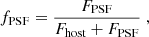
While IllustrisTNG includes SMBH feedback in their physical models, the simulated images produced do not include the light emission from the possible presence of AGN; therefore, we needed to add the contribution of the AGN by injecting a PSF component at varying contribution levels. The PSF contribution fraction (i.e. contribution to the total light) can be defined as
 (3)
(3)
where FPSF is the aperture flux of the PSF component and Fhost is the aperture flux of the host galaxy. We want to create a diverse training sample with different values of fPSF. To do so, we injected a central point source at different levels into the host galaxy image. The observed Euclid PSF effective models (Cropper et al. 2016) were used as the central point source. For each galaxy, five different images were created with five different fPSF values, chosen randomly in the range [0, 1). The PSF-injected images were created as follows:
-
a random PSF was selected;
-
the flux of the PSF and the host galaxy was measured within an aperture of 0
 5 radius for all galaxies, using the aperturephotometry function of the photutils package (Bradley et al. 2024);
 -
the PSF image was scaled to satisfy Eq. (3), for a chosen fPSF;
-
the scaled PSF image was added to the host galaxy image, at the centre of the galaxy.
We chose this aperture to capture the majority of the galaxy flux for most sources. This is particularly true at the highest redshifts, where most galaxies above the stellar mass limit are smaller than our aperture (van der Wel et al. 2014). However, at lower redshifts, an increasing number of galaxies exceed the aperture size, potentially leading to a slight overestimation of fPSF. Conversely, selecting a larger aperture to accommodate these extended low-redshift galaxies could introduce flux contamination from nearby sources, biasing fPSF towards lower values. Finding an optimal aperture across a wide redshift range is challenging, and we leave a more detailed exploration of aperture selection to future work. We note that the observed VIS flux corresponds to different rest-frame wavelengths depending on redshift: the central wavelength of the VIS filter samples rest-frame around 240 nm at z = 2, and 480 nm at z = 0.5. In the future, incorporating SED modelling may be a promising way forwards to infer the PSF contribution fraction at a common rest-frame wavelength. However, in this work, we focus solely on the observed wavelength range. This procedure resulted in a final sample of 750 000 mock galaxies with different levels of fPSF. Example images of these simulated galaxy images with varying levels of fPSF can be seen in Fig. 3. It is clear that as we increase the relative contribution of the PSF, the galaxy image becomes increasingly more dominated by an unresolved point source.
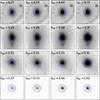 |
Fig. 3. Example mock Euclid VIS images with varying levels of PSF contribution (fPSF) to the total flux. The images were generated to mimic Euclid observations and include realistic Euclid noise and background. Each row corresponds to a different galaxy, with increasing PSF contribution fractions from left to right, at different magnitudes. The images correspond to a physical size of around 25 kpc and are displayed with an inverse arcsinh scaling. The blue circles show an aperture of 0 |

3.2. Deep learning model and training
Zoobot (Walmsley et al. 2023) is a Python package used to measure detailed morphologies of galaxies with DL. Zoobot includes different DL architectures pre-trained on millions of labelled galaxies, derived from visual classifications of the Galaxy Zoo project (Lintott et al. 2008) on real images of galaxies selected from surveys such as the Sloan Digital Sky Survey (SDSS), Hyper Suprime-Cam (HSC), and Hubble (Willett et al. 2013, 2017; Simmons et al. 2017; Walmsley et al. 2022a,b; Omori et al. 2023). The models can be adapted to new tasks and new galaxy surveys without needing a large amount of labelled data, since they rely on the learned representations. This process, known as ‘transfer learning’ (Lu et al. 2015), allows a previously trained machine-learning model to be applied to a new problem. Instead of retraining all parameters from scratch, the existing model architecture and learned weights from prior training can be re-used, making adaptation more efficient.
For this work, to train a DL model to predict the PSF contribution fraction, fPSF, from a galaxy image, we followed the same procedure as in Margalef-Bentabol et al. (2026). We used a ConvNeXt (Liu et al. 2022) model, in particular, the ConvNeXt-Base architecture, which consists of 36 convolutional blocks that are designed to resemble transformer blocks, while maintaining the efficiency of CNNs pre-trained on the Galaxy Zoo data set of over 820 000 images and 100 million volunteer votes to morphological questions. ConvNext architectures incorporate enhancements inspired by transformer models (Dosovitskiy et al. 2021) into traditional convolutional networks, resulting in improved performance and efficiency for vision-based tasks. We adapted the model to perform a regression task by replacing the original model head (top layer) with a single dense layer with one neuron (corresponding to the predicted output of the network), using a sigmoid activation function for the final layer (to restrict the output between 0 and 1), and a mean-square-error loss function to train the network. First, we loaded the pre-trained parameters of the architecture. Then, we retrained the last four blocks and the linear head, while keeping the rest of the network’s parameters frozen to the optimal values found for the pre-trained data from Galaxy Zoo. Our sample of mock galaxies was split into training, validation, and test sets, containing 80%, 10%, and 10% of the total sample, respectively. The split was done in such a way that the five iterations of a single galaxy (the mock images of the same galaxy with five different levels of the PSF component injected) were only contained in one of the splits. The training and validation data sets were used during training and to optimise the model’s hyperparameters, while the test data set was only used to evaluate the best-performing model presented here. The model was trained on a V100 GPU and took 24 hours to complete.
4. Results
In this section, we first analyse the overall performance of our DL model in estimating fPSF, using common metrics for regression tasks such as the root mean square error (RMSE), the relative absolute error (RAE), and the outlier fraction. Then we present an analysis of how our method compares with other AGN selection techniques, and how the overlaps with other selections change with respect to AGN properties such as their luminosity and relative dominance compared to the host galaxy. Finally, we examine the dependence of our DL-identified AGN on the host galaxy stellar mass and location in the star-formation main sequence (SFMS) diagram.
4.1. Zoobot model performance
We analysed the performance of the trained DL model on the test data constructed from the TNG simulations, evaluating its ability to predict the PSF contribution fraction (fPSF. The bottom panel of Fig. 4 shows the predicted fPSF versus the injected fPSF (i.e. the true value), colour-coded by the number density of objects. It is evident that the vast majority of the objects lie close to the 1:1 line across the whole range of the injected fPSF, demonstrating that the model is able to recover the true fPSF with high accuracy and precision. For galaxies with fPSF [injected] < 0.05, for which the mean difference between the predicted and true fPSF is larger, only around 5% of them have fPSF [predicted] > 0.2 and 0.4% have fPSF [predicted] > 0.5. Furthermore, the galaxies with the largest differences tend to be in the highest redshift bins and appear to be compact sources. As is shown in Margalef-Bentabol et al. (2026), when sources are very compact, and possibly unresolved, this method will not give accurate results in terms of the predicted fPSF. The top panel of Fig. 4 shows the mean difference between the real and predicted values (ΔfPSF = fPSF [injected] −fPSF [Zoobot]) and its dispersion as a function of the injected fPSF. The mean bias across the whole test set is ⟨ΔfPSF⟩= − 0.0078. When the intrinsic PSF contribution is very low (i.e. fPSF [injected] < 10%), the difference ΔfPSF starts to increase (to −0.06 in the lowest fPSF [injected] bin), with a slight overestimation in the predicted fPSF. The dispersion also increases with decreasing fPSF [injected], from 0.02 to 0.14.
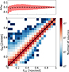 |
Fig. 4. Comparison between the injected PSF contribution fraction and the predicted contribution fraction from Zoobot on the test set across the whole redshift range (0.5 < z < 2). The diagonal line is the 1:1 relation. The top plot shows the mean difference and the standard deviation as a function of the injected PSF contribution fraction. The colour bar indicates the number of sources in each 2D bin. |
We further analysed the RMSE, RAE, and outlier fraction as a function of different properties, including the injected (i.e. true) fPSF, redshift, S/N, and size. The RMSE can be derived as follows:
![Mathematical equation: $$ \begin{aligned} \mathrm{RMSE} = \sqrt{\frac{1}{n}\sum _{i = 1} ^{n} (f^i_{\rm PSF} [\mathrm{injected}] - f^i_{\rm PSF} [\mathrm{predicted}])^2}\;, \end{aligned} $$](/articles/aa/full_html/2026/07/aa54583-25/aa54583-25-eq10.gif) (4)
(4)
which measures the average difference between the predicted values and the actual injected values. The RAE is the ratio between the absolute error and the real value,
![Mathematical equation: $$ \begin{aligned} \mathrm{RAE} = \frac{|f_{\rm PSF}[\mathrm{injected}] - f_{\rm PSF} [\mathrm{predicted}] |}{f_{\rm PSF} [\mathrm{injected}]}\;. \end{aligned} $$](/articles/aa/full_html/2026/07/aa54583-25/aa54583-25-eq11.gif) (5)
(5)
Note that the RAE is not well defined when the real fPSF is equal to zero; therefore, we did not calculate the RAE in that case. Based on the RAE, we can also define the outlier fraction in the Zoobot predictions, as the fraction of galaxies that have a RAE higher than a given threshold (toutlier). That is the fraction of galaxies that satisfy
 (6)
(6)
with the adopted thresholds being 50% in this study (i.e. the prediction error is at least 50%). We used Sextractor to determine the physical size of the simulated galaxy, as measured by the Kron radius (rw), in kiloparsecs. To calculate the S/N, we measured the flux within an aperture of 0 5 centred on the source and divided by the flux corresponding to the background noise in an aperture of the same size in an empty region of the sky near the source.
Our trained DL model has an overall mean value of RMSE = 0.052 and RAE = 0.30. In Fig. 5, we show the RMSE and RAE of the Zoobot predictions as a function of the injected PSF contribution fraction, redshift, S/N, and Kron radius (calculated in the IE filter). The error bars in Fig. 5 represent the 95% confidence interval obtained through bootstrapping. We can see that the RMSE decreases with an increasing contribution from the PSF, which is expected because a more dominant PSF can help us estimate its contribution more precisely. In fact, when fPSF [injected] ≳40%, the precision of fPSF[predicted] is higher than the intrinsic variation (a fractional change of about 13% as is shown in Fig. 1) in the observed Euclid PSF (indicated by the shaded grey region). The RAE increases rapidly with decreasing fPSF [injected], which is expected due to RAE being sensitive to small values of fPSF [injected]. Both the RMSE and RAE increase slowly with increasing redshift (with a minimum value of RMSE of 0.035 at the lowest redshift bin and a maximum of 0.67 at the highest redshift bin), and remain mostly constant with S/N, probably due to the training sample having enough galaxies with a low S/N. The RMSE increases with decreasing galaxy size (with a minimum value of 0.36 for larger galaxies and a maximum of 0.74 for the smallest ones), which can be explained by the fact that it is more difficult to estimate fPSF precisely in more compact galaxies.
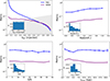 |
Fig. 5. RMSE and average RAE as a function of the injected PSF contribution fraction (top left panel), redshift (top right), S/N (bottom left), and size (bottom right). The error bars show the 95% interval from bootstrapping. The insets show the distribution of each quantity. The grey area of the top left panel corresponds to the level of the intrinsic fractional variation (standard deviation divided by the mean), considering the spatial and temporal variations in the observed Euclid VIS PSF. |
The overall outlier fraction is 8 ± 1%, based on outliers defined as those with RAE > 50%. This definition of outlier fraction is most sensitive to smaller values of the true fPSF and can miss large absolute errors; that is why we also adopted another definition for selecting outliers based on the residuals, and using the overall RMSE value of 0.052. We define as outliers those galaxies for which the difference between the predicted and true fPSF is more than 5σ (i.e. > 0.26). Based on this alternative definition, we find an overall outlier fraction of 0.43 ± 0.03%. In Fig. 6 we show how the two different outlier fractions change as a function of the fPSF [injected], redshift, S/N, and galaxy size. The residual-based outlier fraction generally increases with decreasing fPSF [injected], increasing z, and galaxy size, while remaining relatively constant with S/N. The outlier fraction based on RAE increases more drastically with decreasing fPSF, as was expected, and only slightly with increasing z, while remaining constant with S/N and galaxy size.
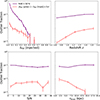 |
Fig. 6. Similar to Fig. 5, but for the outlier fraction, calculated as the fraction of galaxies with RAE > 50% or |
![Mathematical equation: $ |f_{\mathrm{PSF}} [\rm predicted]-f_{\mathrm{PSF}} [\rm true]| > 5\,\sigma $](/articles/aa/full_html/2026/07/aa54583-25/aa54583-25-eq14.gif)
4.2. Comparison with other AGN selections
We applied the trained DL model to our stellar-mass-selected sample of real Euclid galaxies described in Sect. 2.3. Figure 7 shows the cumulative distribution of the estimated fPSF for the whole sample across the EDFs. Traditional methods typically adopt a binary AGN versus non-AGN classification, but it has been shown that, for massive galaxies, the AGN fraction depends on the sensitivity of the survey (Sabater et al. 2019). With our approach, by estimating the AGN contribution fraction, we can move beyond this simplistic binary classification. Galaxies can, instead, be classified as AGN candidates based on a specific threshold of the fractional PSF contribution. While these AGN candidates have a measurable contribution from the PSF, they need to be confirmed as AGN, since other compact central sources, such as stellar clusters or starburst regions, particularly at high redshift, may remain unresolved and contribute to the detected PSF contribution fraction in our method. We can select the most appropriate threshold for a given science case, whether we aim to focus on more dominant AGN or include galaxies with lower AGN contributions. First, we applied a threshold of fPSF > 0.2 to classify AGN candidates. This threshold, chosen as a conservative cut (approximately 4σ), is based on the overall RMSE of the model. Using this criterion, our model identifies 61 432 ± 70 galaxies that are classified as AGN over the entire area of the EDFs by our model, which represents 9.8 ± 0.1% of our whole stellar-mass-limited sample and corresponds to 972 ± 2 deg−2. To estimate the number of AGN candidates, we performed Monte Carlo realisations of the fPSF values by sampling from a Gaussian distribution, where the width of the distribution was set to the RMSE value. The mean of these realisations represents the value of the classified AGN candidates, while the standard deviation of the realisations determines the error. We also adopted a less conservative cut at fPSF > 0.1, motivated by the fact that the mean difference between the predicted fPSF and the true fraction is close to zero in this regime, as is demonstrated in Fig. 4. Adopting this cut, we find a total of 188 142 ± 79 AGN in the EDFs, representing 30.1 ± 0.1% of the whole stellar-mass-limited sample and corresponding to 2977 ± 2 deg−2. This highlights the power of our method in identifying an unprecedentedly large sample of AGN-hosting galaxies, spanning a wide range in the relative dominance of the central point source, by selecting more AGN candidates with a measurable AGN component than other methods we compare against, whose numbers are shown in Table 1. Furthermore, there are 1404 ± 11 galaxies with fPSF > 0.5; that is to say, galaxies in which the AGN outshines the host galaxy. This number corresponds to 22 ± 1 of such AGN per deg2.
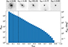 |
Fig. 7. Distribution of fPSF for the whole Euclid stellar-mass-selected sample of galaxies with 0.5 < z < 2 and log10(M*/M⊙) > 9.8. The vertical dashed lines represent the two adopted thresholds above which we classify galaxies as AGN according to the DL model, for the purpose of comparing with other AGN-selection methods. |
To compare our AGN based on the estimated fPSF with AGN samples selected using other selection criteria in Sect. 2.3, we summarise in Table 2 the percentage of AGN in each selection that are also selected as AGN by our DL model. Using the cut at fPSF > 0.2, 34% of the X-ray AGN from the combined 4XMM and CSC2 surveys and 48% of the X-ray AGN from the EROMAIN survey are also selected as AGN based on the estimated fPSF. The larger overlap with the EROMAIN AGN sample is possibly due to the fact that these X-ray AGN are more luminous than the ones from XMM and Chandra (as is shown in Fig. 2). With respect to the MIR-selected AGN, 32% (15%) of the AGN selected by the R90 (C75) diagnostic are also selected by our method. The smaller overlap with the C75-selected MIR AGN is consistent with the fact that this selection has a higher contamination rate compared to the R90 selection. Finally 36% of DESI spectroscopic AGN are also identified as AGN according to our selection based on PSF fraction. However, when considering only the QSO subclass within the DESI spectroscopic AGN, 81% meet our selection criteria. If we use a less conservative cut at fPSF > 0.1, then the overlapping fractions increase significantly for all three AGN selections (i.e. X-ray detection, MIR colour, and optical spectroscopy), with 33% overlap with the C75-selected MIR AGN and 69% overlap with the EROMAIN X-ray AGN at the two extreme ends (the overlap with the QSO sample increases to 89%).
Percentage of AGN from each selection method that we also identified as AGN using a cut on the PSF contribution fraction.
In Fig. 8 we show the normalised distributions of the predicted fPSF in the different AGN samples. The X-ray-selected AGN are the most common AGN population among galaxies with higher PSF contribution fractions (fPSF > 0.3), indicating a better correspondence with optically dominant AGN (which would be naturally linked to less dust-obscured AGN; see Euclid Collaboration: Roster et al. 2026). For comparison, we also plot the distribution of the predicted fPSF in what we call the non-AGN sample. These non-AGN galaxies are, by construction, not identified as X-ray or MIR AGN in a small sky area (RA = [51.7, 53.7], Dec = [ − 29, − 28]) for which we have both X-ray and MIR coverage. Unfortunately DESI does not overlap with the X-ray surveys in the EDFs. We can see that, while reassuringly a large fraction (over 70%) of the non-AGN have fPSF < 0.1, a small fraction (around 9%) of them do have predicted fPSF > 0.2, indicating that they could in fact be AGN that are missed by the X-ray and MIR selections. In future work, we shall investigate whether these AGN are picked up by other selection techniques; for example, using deeper IRAC MIR data, radio data, or spectroscopic data. Additionally, we explore the most AGN-dominated galaxies in our sample that lack counterparts in the comparison methods. In Fig. A.1, we present the properties of galaxies with fPSF > 0.7 (purple histograms) and find that they tend to be less massive and fainter than AGN selected by other methods. This suggests that our approach is particularly effective at detecting AGN activity in lower-mass and fainter galaxies, where traditional selection techniques may be less sensitive. Despite their lower overall luminosity, these AGN can still exhibit a very strong central contribution in the VIS filter, as is reflected by their high PSF contribution fraction. This result opens a new parameter space for studying AGN in lower-mass galaxies, providing valuable insights into SMBH growth in this regime.
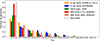 |
Fig. 8. Fraction of galaxies in bins of the predicted PSF contribution fraction in the AGN samples from different selections (X-ray detection, MIR colours, and optical spectroscopy) and the non-AGN sample (see text in Sect. 2.3). |
For the X-ray-selected AGN, clearly the more luminous ones detected in EROMAIN have systematically higher fPSF values. Similarly, for the MIR-selected AGN, the distribution corresponding to the R90 selection, which includes more secure and possibly brighter AGN than the C75 selection, is systematically skewed towards higher fPSF values. However, a large fraction of the X-ray-selected, MIR, and DESI spectroscopic AGN exhibit significantly lower fPSF values, as is seen in Fig. 8, indicating that they are more likely to be obscured by dust. These galaxies show little to no contribution from the central point-source component in the IE images, which explains the low predicted fPSF values despite their classification as AGN from their respective selections. This can be seen clearly in Figs. A.2, A.3, and A.4, where random examples of each AGN type with fPSF < 0.1 are shown. Many of these galaxies display spiral, clumpy, or edge-on morphologies, which are expected to have a higher dust content.
We can use the PSF contribution fraction to estimate the AGN luminosity, defined as the luminosity of the PSF component LPSF in the EuclidIE filter and calculated as
 (7)
(7)
where Ltotal is the total luminosity of a galaxy in the IE filter, estimated from the total flux derived in Euclid Collaboration: Romelli et al. (2026). We show the relation between LPSF and the X-ray luminosity in the top panel of Fig. 9. We fitted a linear relation to each X-ray sample and found  for the EROMAIN sample and
  for the 4XMM&CSC2 sample. Considering the full X-ray sample, we obtained
  . The bottom panel in Fig. 9 shows the fraction of AGN identified using our method based on fPSF as a function of the adopted cut on the X-ray luminosity, LX, for the X-ray sample, or the AGN bolometric luminosity, Lbol, for AGN selected in the X-ray or via DESI optical spectroscopy. We see that the fraction of AGN selected by our model increases with increasing LX. This is expected because LX generally correlates with the luminosity from the PSF component in the VIS images, albeit with significant scatter. For the DESI spectroscopic AGN, estimates of Lbol have been estimated through SED fitting (Siudek et al. 2024). To convert from LX to Lbol, we followed the luminosity-dependent correction presented in Shen et al. (2020):
![Mathematical equation: $$ \begin{aligned} \frac{L_{\rm bol}}{L_{\rm X\,[0.5-2\,\mathrm{keV}]}} = c_1 \left( \frac{L_{\rm bol}}{10^{10}L_{\odot }} \right)^{k_1} + c_2 \left( \frac{L_{\rm bol}}{10^{10}L_{\odot }} \right)^{k_2}\;, \end{aligned} $$](/articles/aa/full_html/2026/07/aa54583-25/aa54583-25-eq19.gif) (8)
(8)
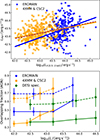 |
Fig. 9. X-ray and bolometric luminosity relations. The top panel shows the AGN luminosity, LPSF, as a function of X-ray luminosity, LX, for the EROMAIn sample (blue circles) and the 4XMM&CSC2 sample (orange squares). The solid blue and orange lines represent the best linear fit to each sample, respectively, while the dotted purple line is the best fit to the whole X-ray sample. The bottom panel shows the overlapping fraction of AGN as a function of the adopted cut on the X-ray luminosity (for the X-ray sample) or the bolometric luminosity (for the DESI spectroscopic sample, in green). The solid lines show the overlapping fraction of AGN defined by fPSF > 0.2, while the dashed lines show the fraction if we select AGN as defined by fPSF > 0.1. |
where c1 = 5.712, k1 = −0.026, c2 = 12.60, and k2 = 0.278. Again, we see a generally increasing fraction of AGN identified based on fPSF with increasing Lbol.
4.3. Dependence on stellar mass and SFR
Many previous studies have shown that the X-ray luminosity or the SMBH accretion rate increases with increasing host galaxy stellar mass across a wide range of redshifts (e.g. Mullaney et al. 2012; Rodighiero et al. 2015; Aird et al. 2018; Yang et al. 2018a; Carraro et al. 2020). Therefore, we first analysed whether stellar mass plays a major role in determining how luminous the AGN is (as a proxy for the growth rate of the SMBH) in a galaxy, and whether there is any significant redshift evolution.
In Fig. 10 we show the luminosity of the AGN, which corresponds to the luminosity of the PSF component, LPSF, in the EuclidIE filter, calculated from Eq. (7) as a function of stellar mass and redshift. The panels show the 2D histogram of the AGN luminosity and stellar mass in six redshift bins. At all redshifts, we observe a broad positive correlation between LPSF and stellar mass, supporting previous claims that SMBHs generally grow faster (in absolute terms, i.e. the luminosity of the PSF component is larger) in more massive systems. This could be due to a larger supply of gas in more massive galaxies and/or a more efficient way of transporting the gas to the central region (e.g. galaxy mergers and the presence of compact cores, which are more prevalent in galaxies with larger stellar masses). We parameterised this correlation in each redshift bin by fitting a log-log linear function (log10LPSF erg s−1] = a log10 M∗[M⊙] + b) and report the best-fit parameters and their uncertainties in Table 3. Based on the best-fit values, we also derived another set of fits by fixing the slope, a, at 0.59. This choice is motivated by the fact that, at higher redshifts, detecting fainter AGN becomes progressively more challenging, as is shown in Fig. 10, where the lower boundary of the distribution shifts upwards with increasing redshift. This effect could potentially lead to an artificial flattening of the slope. By fixing it to the value derived from the more complete lower-redshift bin, we ensure that any observed evolution is reflected in the normalisation rather than in a potentially biased slope. This positive correlation between AGN luminosity and galaxy stellar mass bears similarity to the well-studied SFMS (e.g. Brinchmann et al. 2004; Elbaz et al. 2007; Speagle et al. 2014; Pearson et al. 2018; Popesso et al. 2023), suggesting that a common supply of gas could be used to fuel both the assembly of the SMBH and the host galaxy. In addition, we also observe a mild redshift evolution in the LPSF versus stellar mass relation, indicating that SMBHs grow faster in host galaxies at the same mass at higher redshifts. This behaviour is also qualitatively similar to the observed redshift evolution of the SFMS, which could be partly explained by an increasing molecular gas fraction at higher redshifts (Scoville et al. 2017; Liu et al. 2019; Tacconi et al. 2020; Wang et al. 2022). Our results, based on the PSF contribution fraction as a proxy for AGN activity, show qualitative agreement with previous studies that measure the average black hole accretion rate (BHAR) as a function of stellar mass, revealing the existence of an ‘AGN main sequence’, a term introduced in Mullaney et al. (2012) and further explored in subsequent works (e.g. Yang et al. 2018b; Guetzoyan et al. 2025; Zou et al. 2024). In this work, we do not calculate BHAR because a reliable conversion from the VIS luminosity in the observed frame to the bolometric luminosity of the AGN is not yet established. In a future work, we plan to investigate how to determine BHAR from LPSF by first establishing a conversion between LPSF and the bolometric luminosity. This may be done, for example, through calibration with X-ray measurements or SED fitting. However, our current comparison of LPSF with X-ray luminosities shows only a weak correlation with substantial scatter, suggesting that a robust calibration is non-trivial and may depend on redshift. Developing such a calibration will allow us to compare more quantitatively with studies that derive BHAR from bolometric luminosity estimates under an assumed radiative efficiency. Nonetheless, the PSF luminosity, LPSF, can be interpreted as a proxy for BHAR. In addition, the positive correlation that we find in Fig. 10 between LPSF and stellar mass is qualitatively consistent with the positive correlation between the mean BHAR and stellar mass found in these studies.
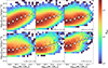 |
Fig. 10. 2D histogram of the AGN luminosity (luminosity in the IE filter multiplied by fPSF) versus stellar mass, in different redshift bins, for all galaxies in our mass-limited sample. The white stars show the mean value, and the error bars show the dispersion of the data. The colours of the 2D histogram show the number of points in each bin. |
Best-fit parameters for the log10(LPSF/[erg s−1]) versus log10(M*/[M⊙]) linear relation, in different redshift bins.
Mullaney et al. (2012), on the other hand, measured the average X-ray luminosity (LX) as a function of stellar mass, finding a positive correlation with a slope of 0.86 ± 0.39 for their sample at z ∼ 1, and a slope of 1.05 ± 0.36 for their z ∼ 2 sample. In our case, we measured LPSF as a function of stellar mass, but from Fig. 9 we inferred a relation between LPSF and LX of  . Converting the relations from Mullaney et al. (2012) to the corresponding LPSF scaling via the LPSF–LX relation, we obtained
  for their z ∼ 1 sample and
  for z ∼ 2 sample. To allow for a direct comparison, we divided our sample into a lower-redshift bin (0.5 < z < 1.25), comparable to Mullaney et al. (2012)’s z ∼ 1 sample, and a higher-redshift bin (1.25 < z < 2), comparable to their z ∼ 2 sample. We find
  at lower redshift and
  at higher redshift. For the lower-redshift bin, our slope is slightly steeper but still consistent, within the uncertainties, with that derived from Mullaney et al. (2012). For the higher-redshift bin, our results are fully consistent within the errors. It is worth noting, however, that the Mullaney et al. (2012) sample includes only star-forming galaxies, whereas our sample is not restricted to star-forming systems. Several studies have also shown differences in the correlation between SMBH accretion rates and host galaxy stellar mass in different galaxy types (Carraro et al. 2020; Aird et al. 2022). For example, star-forming galaxies are shown to have steeper slopes than quiescent galaxies. Given that the fraction of quiescent galaxies also evolves with redshift, we defer a proper characterisation of the evolution in the LPSF versus stellar mass relation to a future work in which we can reliably separate different galaxy types.
Lastly, we explore the connection between AGN identified based on the contribution of the PSF component and their location in the SFR versus stellar mass plane. Figure 11 shows the 2D histogram of SFR versus stellar mass, in different redshift bins, colour-coded by the median fPSF (left panel) and the median log10LPSF. Only bins with at least ten galaxies are plotted. The Popesso et al. (2023) SFMS is also over-plotted in all redshift bins. We can see that, in terms of the relative contribution fraction of the AGN (as characterised by fPSF), quiescent galaxies (i.e. galaxies significantly offset below the SFMS), or galaxies at the high-mass end (across the full range in the specific SFR, i.e. SFR divided by stellar mass) tend to be more dominated by their AGN. In terms of the absolute power of the AGN (as characterised by LPSF), the starburst galaxies (i.e. galaxies above the SFMS) or very massive galaxies tend to host the most powerful AGN. The observation that starburst galaxies can host very powerful AGN might indicate that rapid build-up of the SMBH and the host galaxy can occur concomitantly. Galaxy mergers provide a possible pathway for this coevolution by funnelling gas into the central regions, triggering intense star formation while also fuelling the SMBH’s growth. In Fig. 12, we plot the 2D histogram of SFR versus stellar mass, colour-coded by the fraction of galaxies with fPSF > 0.2 (top panel), fPSF > 0.4 (middle panel), and fPSF > 0.6 (bottom panel). We can see that while a larger fraction of the quiescent galaxies host AGN (defined by fPSF > 0.2 in this work) compared to the star-forming galaxy population, this is not the case in the highest redshift bins (where the fraction of quiescent galaxies is very small). This could indicate that, while at high redshift star-forming galaxies and their central SMBHs grow together, at lower redshifts this co-evolution weakens, and AGN instead play a role in the quenching of galaxies by suppressing star formation. We observe the same trend with different thresholds of fPSF, as is shown by the different panels in Fig. 12. We note, however, that the high fraction of low-mass quiescent galaxies with fPSF > 0.2 should be interpreted with caution. While these AGN candidates have a measurable PSF contribution, they still need to be confirmed as AGN, since other compact central sources, such as stellar clusters or starburst regions, may remain unresolved, particularly in faint and compact galaxies, and could contribute to the detected PSF fraction in our method. Another cautionary note to consider is that stellar masses and SFRs are currently estimated without accounting for the potential contribution of the AGN component in a galaxy. Future works should focus on deriving physical properties that incorporate the AGN contribution for more accurate results.
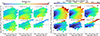 |
Fig. 11. 2D histogram of SFR versus stellar mass in different redshift bins. Each 2D bin is colour-coded by the median value of fPSF (left) or the median value of log10(LPSF) (right) of all galaxies from our mass-limited sample in that bin. The black lines show the Popesso et al. (2023) SFMS at the median redshift of the bin. Only bins with at least ten galaxies are plotted. |
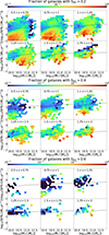 |
Fig. 12. Similar to Fig. 11, but colour-coded by the fraction of galaxies with fPSF > 0.2 (top), fPSF > 0.4 (centre), and fPSF > 0.6 (bottom). |
5. Conclusions
We have presented a DL-based image decomposition method to quantify the AGN contribution, which is calculated as the contribution of the point-source component (fPSF) in galaxy imaging data. We trained the DL model with a large sample of mock galaxy images, produced from the TNG simulations to mimic the Euclid VIS observations and with artificially injected AGN, in the form of varying fPSF. We applied the trained model to estimate fPSF in a stellar-mass-limited sample of galaxies selected from the Euclid Q1 data. Our main findings are the following.
-
The DL model trained on the mock data is able to recover the intrinsic contribution of the PSF, with high precision and accuracy. The mean difference between the true and predicted fPSF is −0.0078. The overall mean RMSE and RAE are 0.052 and 0.30, respectively. The outlier fraction defined as RAE > 50% (difference > 5σ) is 8.0 ± 0.1% (0.43 ± 0.03%). In addition, when the intrinsic fPSF is > 40%, the precision of our method exceeds the level of the intrinsic variation in the observed Euclid VIS PSF.
-
Based on the estimated AGN contribution, 9.8 ± 0.1% galaxies can be classified as AGN in the Euclid sample across the EDFs, if we impose a condition of fPSF > 0.2. By adopting a less conservative threshold of fPSF > 0.1, we can identify a total of 30.1 ± 0.1% AGN. Because our DL-based method can select AGN even if the AGN component is not the main contributor to the luminosity of the host galaxy, this technique gives many more AGN compared to the other AGN-selection methods explored in this study. In addition, we can go beyond a simple binary AGN or non-AGN classification by quantifying the contribution of the AGN.
-
We compared our AGN sample selected using cuts on fPSF with other commonly used AGN selections, based on X-ray detections, MIR colours, and optical spectroscopy. We find that 15–48% of the AGN (depending on the specific selection technique) are also selected as AGN by our criterion (fPSF > 0.2). The overlap increases to 33–69% when we select our AGN using a less conservative criterion fPSF > 0.1. In addition, we find that the overlap increases with an increasing X-ray luminosity (for the X-ray AGN) or bolometric AGN luminosity (for the DESI spectroscopic AGN).
-
Galaxies with higher stellar masses tend to host more luminous AGN (i.e. a more luminous point source), indicating faster growth (in absolute terms) of the SMBH in more massive systems. The correlation also seems to evolve mildly with redshift, with AGN becoming more luminous at higher redshifts.
-
We find that quiescent galaxies are more likely to host AGN (as determined by our DL method) compared to star-forming galaxies, particularly at lower redshifts, with a stronger dominance of the AGN in terms of its contribution to the total observed light. This suggests that the presence of AGN is closely linked to the quenching process in galaxy evolution.
-
The most massive and starbursting galaxies host the most luminous AGN, suggesting that these galaxies undergo a phase of intense SMBH growth alongside starburst activity. Additionally, the higher number of galaxies with fPSF > 0.2 above and along the SFMS suggests that many star-forming galaxies and starbursts undergo a crucial AGN phase in their evolutionary path, highlighting the interplay between galaxy formation, starburst activity, and black hole growth.
In a future work, we shall extend this DL-based approach to higher redshifts and the Euclid NISP bands, for which the model can easily be adapted and output fPSF predictions of thousands of galaxies in a few seconds, making it an ideal method for future data releases from Euclid. With the future data releases covering significantly larger areas, we shall also extend the comparison of our AGN sample to AGN selected with other techniques, such as radio-selected AGN, Euclid type I and type II AGN, and variability-selected AGN. This will also allow us to better investigate galaxies with high fPSF that are not classified as AGN by any of the methods presented here. By examining whether these galaxies are detected through alternative selection techniques or remain uniquely identified by our approach, we can explore the nature of this potential new population of AGN candidates and assess their role in galaxy evolution. A complementary approach would be to follow up a subset of these sources at higher resolution to determine whether some fraction of the PSF contribution originates from compact galactic cores rather than AGN. Such an investigation would provide further insight into the nature of these objects. In the current work, our estimates of the photo-zs and galaxy physical properties such as stellar mass and SFR are not optimised for galaxies with a dominant AGN. For future analysis, using our method, we can remove the contribution of the AGN in the photometric bands and then carry out SED fitting using the decomposed photometric measurements to obtain more reliable photo-z and physical property estimates. Consequently, we can properly study the co-evolution of the growth of the SMBHs and their host galaxies in different galaxy populations (i.e. star-forming galaxies along the SFMS, starburst galaxies, and quiescent galaxies) and how the relative pace of the two assembly histories evolves with cosmic time.
Acknowledgments
The Euclid Consortium acknowledges the European Space Agency and a number of agencies and institutes that have supported the development of Euclid, in particular the Agenzia Spaziale Italiana, the Austrian Forschungsförderungsgesellschaft funded through BMK, the Belgian Science Policy, the Canadian Euclid Consortium, the Deutsches Zentrum für Luft- und Raumfahrt, the DTU Space and the Niels Bohr Institute in Denmark, the French Centre National d’Etudes Spatiales, the Fundação para a Ciência e a Tecnologia, the Hungarian Academy of Sciences, the Ministerio de Ciencia, Innovación y Universidades, the National Aeronautics and Space Administration, the National Astronomical Observatory of Japan, the Netherlandse Onderzoekschool Voor Astronomie, the Norwegian Space Agency, the Research Council of Finland, the Romanian Space Agency, the State Secretariat for Education, Research, and Innovation (SERI) at the Swiss Space Office (SSO), and the United Kingdom Space Agency. A complete and detailed list is available on the Euclid web site (www.euclid-ec.org). This work has made use of the Euclid Quick Release Q1 data from the Euclid/ mission of the European Space Agency (ESA), 2025, https://doi.org/10.57780/esa-2853f3b. This research makes use of ESA Datalabs (datalabs.esa.int), an initiative by ESA’s Data Science and Archives Division in the Science and Operations Department, Directorate of Science. Based on data from UNIONS, a scientific collaboration using three Hawaii-based telescopes: CFHT, Pan-STARRS, and Subaru (www.skysurvey.cc ). Based on data from the Dark Energy Camera (DECam) on the Blanco 4-m Telescope at CTIO in Chile (https://www.darkenergysurvey.org ). Based on data from the ESA mission Gaia, whose data are being processed by the Gaia Data Processing and Analysis Consortium (https://www.cosmos.esa.int/gaia ). This publication is part of the project “Clash of the Titans: deciphering the enigmatic role of cosmic collisions” (with project number VI.Vidi.193.113 of the research programme Vidi, which is (partly) financed by the Dutch Research Council (NWO). This research was supported by the International Space Science Institute (ISSI) in Bern, through ISSI International Team project #23-573 "Active Galactic Nuclei in Next Generation Surveys". We thank the Center for Information Technology of the University of Groningen for their support and for providing access to the Hábrók high-performance computing cluster. We thank SURF (www.surf.nl) for the support in using the National Supercomputer Snellius.
References
- Aird, J., Coil, A. L., Moustakas, J., et al. 2012, ApJ, 746, 90 [CrossRef] [Google Scholar]
- Aird, J., Coil, A. L., & Georgakakis, A. 2018, MNRAS, 474, 1225 [NASA ADS] [CrossRef] [Google Scholar]
- Aird, J., Coil, A. L., & Kocevski, D. D. 2022, MNRAS, 515, 4860 [NASA ADS] [CrossRef] [Google Scholar]
- Antonucci, R. 1993, ARA&A, 31, 473 [Google Scholar]
- Assef, R. J., Prieto, J. L., Stern, D., et al. 2018, ApJ, 866, 26 [NASA ADS] [CrossRef] [Google Scholar]
- Azadi, M., Coil, A. L., Aird, J., et al. 2017, ApJ, 835, 27 [NASA ADS] [CrossRef] [Google Scholar]
- Beifiori, A., Courteau, S., Corsini, E. M., & Zhu, Y. 2012, MNRAS, 419, 2497 [NASA ADS] [CrossRef] [Google Scholar]
- Bianchi, S., Mainieri, V., & Padovani, P. 2022, in Handbook of X-ray and Gamma-ray Astrophysics, eds. C. Bambi, & A. Santangelo (Singapore: Springer Nature Singapore), 1 [Google Scholar]
- Bradley, L., Sipőcz, B., Robitaille, T., et al. 2024, https://doi.org/10.5281/zenodo.10967176 [Google Scholar]
- Brinchmann, J., Charlot, S., White, S. D. M., et al. 2004, MNRAS, 351, 1151 [Google Scholar]
- Bruzual, G., & Charlot, S. 2003, MNRAS, 344, 1000 [NASA ADS] [CrossRef] [Google Scholar]
- Carraro, R., Rodighiero, G., Cassata, P., et al. 2020, A&A, 642, A65 [EDP Sciences] [Google Scholar]
- Cid Fernandes, R., Stasińska, G., Schlickmann, M. S., et al. 2010, MNRAS, 403, 1036 [Google Scholar]
- Cropper, M., Pottinger, S., Niemi, S., et al. 2016, SPIE Conf. Ser., 9904, 99040Q [NASA ADS] [Google Scholar]
- DESI Collaboration (Adame, A. G., et al.) 2024, AJ, 168, 58 [NASA ADS] [CrossRef] [Google Scholar]
- Dosovitskiy, A., Beyer, L., Kolesnikov, A., et al. 2021, ArXiv e-prints [arXiv:22010.11929] [Google Scholar]
- Elbaz, D., Daddi, E., Le Borgne, D., et al. 2007, A&A, 468, 33 [NASA ADS] [CrossRef] [EDP Sciences] [Google Scholar]
- Euclid Collaboration (Cropper, M., et al.) 2025, A&A, 697, A2 [Google Scholar]
- Euclid Collaboration (Jahnke, K., et al.) 2025, A&A, 697, A3 [Google Scholar]
- Euclid Collaboration (Mellier, Y., et al.) 2025, A&A, 697, A1 [Google Scholar]
- Euclid Collaboration (Aussel, H., et al.) 2026, A&A, 711, A1 (Euclid Q1 SI) [Google Scholar]
- Euclid Collaboration (Enia, A., et al.) 2026, A&A, 711, A14 (Euclid Q1 SI) [Google Scholar]
- Euclid Collaboration (Matamoro Zatarain, T., et al.) 2026, A&A, 711, A20 (Euclid Q1 SI) [Google Scholar]
- Euclid Collaboration (McCracken, H. J., et al.) 2026, A&A, 711, A2 (Euclid Q1 SI) [Google Scholar]
- Euclid Collaboration (Polenta, G., et al.) 2026, A&A, 711, A3 (Euclid Q1 SI) [Google Scholar]
- Euclid Collaboration (Romelli, E., et al.) 2026, A&A, 711, A4 (Euclid Q1 SI) [Google Scholar]
- Euclid Collaboration (Roster, W., et al.) 2026, A&A, 711, A16 (Euclid Q1 SI) [Google Scholar]
- Euclid Collaboration (Tucci, M., et al.) 2026, A&A, 711, A5 (Euclid Q1 SI) [Google Scholar]
- Euclid Quick Release Q1. 2025, https://doi.org/10.57780/esa-2853f3b [Google Scholar]
- Evans, I. N., Evans, J. D., Martínez-Galarza, J. R., et al. 2024, ApJS, 274, 22 [NASA ADS] [CrossRef] [Google Scholar]
- Ghosh, A., Urry, C. M., Mishra, A., et al. 2023, ApJ, 953, 134 [Google Scholar]
- Graham, A. W., & Scott, N. 2013, ApJ, 764, 151 [Google Scholar]
- Greene, J. E., Strader, J., & Ho, L. C. 2020, ARA&A, 58, 257 [Google Scholar]
- Guetzoyan, P., Aird, J., Georgakakis, A., et al. 2025, MNRAS, 536, 79 [Google Scholar]
- Gültekin, K., Richstone, D. O., Gebhardt, K., et al. 2009, ApJ, 698, 198 [Google Scholar]
- Hickox, R. C., & Alexander, D. M. 2018, ARA&A, 56, 625 [Google Scholar]
- Kormendy, J., & Ho, L. C. 2013, ARA&A, 51, 511 [Google Scholar]
- Lamareille, F. 2010, A&A, 509, A53 [CrossRef] [EDP Sciences] [Google Scholar]
- Läsker, R., Ferrarese, L., van de Ven, G., & Shankar, F. 2014, ApJ, 780, 70 [Google Scholar]
- Laureijs, R., Amiaux, J., Arduini, S., et al. 2011, ArXiv e-prints [arXiv:1110.3193] [Google Scholar]
- Li, J., Silverman, J. D., Ding, X., et al. 2021, ApJ, 918, 22 [NASA ADS] [CrossRef] [Google Scholar]
- Lintott, C. J., Schawinski, K., Slosar, A., et al. 2008, MNRAS, 389, 1179 [NASA ADS] [CrossRef] [Google Scholar]
- Liu, D., Schinnerer, E., Groves, B., et al. 2019, ApJ, 887, 235 [Google Scholar]
- Liu, Z., Mao, H., Wu, C.-Y., et al. 2022, in 2022 IEEE/CVF Conference on Computer Vision and Pattern Recognition (CVPR) (Los Alamitos, CA (USA: IEEE Computer Society)), 11966 [Google Scholar]
- Lu, J., Behbood, V., Hao, P., et al. 2015, Know.-Based Syst., 80, 14 [Google Scholar]
- Mainzer, A., Bauer, J., Grav, T., et al. 2011, ApJ, 731, 53 [Google Scholar]
- Margalef-Bentabol, B., Wang, L., La Marca, A., & Rodriguez-Gomez, V. 2026, A&A, 706, A304 [NASA ADS] [CrossRef] [EDP Sciences] [Google Scholar]
- Marinacci, F., Vogelsberger, M., Pakmor, R., et al. 2018, MNRAS, 480, 5113 [NASA ADS] [Google Scholar]
- Martin, G., Bazkiaei, A. E., Spavone, M., et al. 2022, MNRAS, 513, 1459 [NASA ADS] [CrossRef] [Google Scholar]
- McConnell, N. J., & Ma, C.-P. 2013, ApJ, 764, 184 [Google Scholar]
- Mendez, A. J., Coil, A. L., Aird, J., et al. 2013, ApJ, 770, 40 [Google Scholar]
- Merloni, A., Lamer, G., Liu, T., et al. 2024, A&A, 682, A34 [NASA ADS] [CrossRef] [EDP Sciences] [Google Scholar]
- Mezcua, M., Suh, H., & Civano, F. 2019, MNRAS, 488, 685 [Google Scholar]
- Moustakas, J., Scholte, D., Dey, B., & Khederlarian, A. 2023, Astrophysics Source Code Library [record ascl:2308.005] [Google Scholar]
- Mullaney, J. R., Daddi, E., Béthermin, M., et al. 2012, ApJ, 753, L30 [Google Scholar]
- Naiman, J. P., Pillepich, A., Springel, V., et al. 2018, MNRAS, 477, 1206 [Google Scholar]
- Navarro, V., Del Rio, S., Diego, M. A., et al. 2024, in Space Data Management, ed. A. Cortesi (Singapore: Springer Nature Singapore), 141, 1 [Google Scholar]
- Nelson, D., Pillepich, A., Springel, V., et al. 2018, MNRAS, 475, 624 [Google Scholar]
- Nelson, D., Springel, V., Pillepich, A., et al. 2019, Comput. Astrophys. Cosmol., 6, 2 [Google Scholar]
- Omori, K. C., Bottrell, C., Walmsley, M., et al. 2023, A&A, 679, A142 [NASA ADS] [CrossRef] [EDP Sciences] [Google Scholar]
- Padovani, P., Alexander, D. M., Assef, R. J., et al. 2017, A&ARv, 25, 2 [Google Scholar]
- Pearson, W. J., Wang, L., Hurley, P. D., et al. 2018, A&A, 615, A146 [NASA ADS] [CrossRef] [EDP Sciences] [Google Scholar]
- Peng, C. Y., Ho, L. C., Impey, C. D., & Rix, H.-W. 2002, AJ, 124, 266 [Google Scholar]
- Pillepich, A., Springel, V., Nelson, D., et al. 2018, MNRAS, 473, 4077 [Google Scholar]
- Planck Collaboration XIII. 2016, A&A, 594, A13 [NASA ADS] [CrossRef] [EDP Sciences] [Google Scholar]
- Popesso, P., Concas, A., Cresci, G., et al. 2023, MNRAS, 519, 1526 [Google Scholar]
- Predehl, P., Andritschke, R., Arefiev, V., et al. 2021, A&A, 647, A1 [EDP Sciences] [Google Scholar]
- Ribeiro, B., Le Fèvre, O., Tasca, L. A. M., et al. 2016, A&A, 593, A22 [NASA ADS] [CrossRef] [EDP Sciences] [Google Scholar]
- Rodighiero, G., Brusa, M., Daddi, E., et al. 2015, ApJ, 800, L10 [Google Scholar]
- Rodriguez-Gomez, V., Snyder, G. F., Lotz, J. M., et al. 2019, MNRAS, 483, 4140 [NASA ADS] [CrossRef] [Google Scholar]
- Sabater, J., Best, P. N., Hardcastle, M. J., et al. 2019, A&A, 622, A17 [NASA ADS] [CrossRef] [EDP Sciences] [Google Scholar]
- Scoville, N., Lee, N., Vanden Bout, P., et al. 2017, ApJ, 837, 150 [Google Scholar]
- Shankar, F., Bernardi, M., Sheth, R. K., et al. 2016, MNRAS, 460, 3119 [NASA ADS] [CrossRef] [Google Scholar]
- Shen, X., Hopkins, P. F., Faucher-Giguère, C.-A., et al. 2020, MNRAS, 495, 3252 [Google Scholar]
- Simmons, B. D., Lintott, C., Willett, K. W., et al. 2017, MNRAS, 464, 4420 [Google Scholar]
- Siudek, M., Pucha, R., Mezcua, M., et al. 2024, A&A, 691, A308 [NASA ADS] [CrossRef] [EDP Sciences] [Google Scholar]
- Speagle, J. S., Steinhardt, C. L., Capak, P. L., & Silverman, J. D. 2014, ApJS, 214, 15 [Google Scholar]
- Springel, V., Pakmor, R., Pillepich, A., et al. 2018, MNRAS, 475, 676 [Google Scholar]
- Tacconi, L. J., Genzel, R., & Sternberg, A. 2020, ARA&A, 58, 157 [NASA ADS] [CrossRef] [Google Scholar]
- Toba, Y., Liu, T., Urrutia, T., et al. 2022, A&A, 661, A15 [NASA ADS] [CrossRef] [EDP Sciences] [Google Scholar]
- Ueda, Y., Akiyama, M., Ohta, K., & Miyaji, T. 2003, ApJ, 598, 886 [NASA ADS] [CrossRef] [Google Scholar]
- Urry, C. M., & Padovani, P. 1995, PASP, 107, 803 [NASA ADS] [CrossRef] [Google Scholar]
- van der Wel, A., Franx, M., van Dokkum, P. G., et al. 2014, ApJ, 788, 28 [Google Scholar]
- Walmsley, M., Lintott, C., Géron, T., et al. 2022a, MNRAS, 509, 3966 [Google Scholar]
- Walmsley, M., Scaife, A. M. M., Lintott, C., et al. 2022b, MNRAS, 513, 1581 [NASA ADS] [CrossRef] [Google Scholar]
- Walmsley, M., Allen, C., Aussel, B., et al. 2023, J. Open Source Software, 8, 5312 [NASA ADS] [CrossRef] [Google Scholar]
- Wang, T.-M., Magnelli, B., Schinnerer, E., et al. 2022, A&A, 660, A142 [NASA ADS] [CrossRef] [EDP Sciences] [Google Scholar]
- Webb, N. A., Coriat, M., Traulsen, I., et al. 2020, A&A, 641, A136 [NASA ADS] [CrossRef] [EDP Sciences] [Google Scholar]
- Willett, K. W., Lintott, C. J., Bamford, S. P., et al. 2013, MNRAS, 435, 2835 [Google Scholar]
- Willett, K. W., Galloway, M. A., Bamford, S. P., et al. 2017, MNRAS, 464, 4176 [NASA ADS] [CrossRef] [Google Scholar]
- Wright, E. L., Eisenhardt, P. R. M., Mainzer, A. K., et al. 2010, AJ, 140, 1868 [Google Scholar]
- Yang, G., Brandt, W. N., Darvish, B., et al. 2018a, MNRAS, 480, 1022 [NASA ADS] [CrossRef] [Google Scholar]
- Yang, G., Brandt, W. N., Vito, F., et al. 2018b, MNRAS, 475, 1887 [NASA ADS] [CrossRef] [Google Scholar]
- Zhang, K., & Hao, L. 2018, ApJ, 856, 171 [NASA ADS] [CrossRef] [Google Scholar]
- Zhuang, M.-Y., & Ho, L. C. 2023, Nat. Astron., 7, 1376 [NASA ADS] [CrossRef] [Google Scholar]
- Zou, F., Yu, Z., Brandt, W. N., et al. 2024, ApJ, 964, 183 [NASA ADS] [CrossRef] [Google Scholar]
Appendix A: AGN samples - additional information
We show in Fig. A.1 the distribution of stellar mass, redshift, magnitude in the IE filter and total luminosity of the galaxy in the IE filter (estimated from the total flux derived in Euclid Collaboration: Romelli et al. 2026) for the sample of AGN from the various selections (from X-ray, MIR colours, and DESI spectroscopy). The black histograms represent the samples we refer to as non-AGN (explained in Sect. 2.3). The purple histograms depict the sample of galaxies with fPSF > 0.7 that are not classified as AGN by any other method.
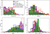 |
Fig. A.1. Normalised distribution of stellar mass (top left), redshift (top right), magnitude (bottom left), and total luminosity (bottom right) for the different types of AGN. |
Figures A.2, A.3, and A.4 show random examples of galaxies selected as X-ray, MIR, and DESI spectroscopic AGN, respectively, for which our DL model predicts low values of PSF contribution fraction (fPSF < 0.1).
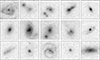 |
Fig. A.2. Example of X-ray AGN with fPSF < 0.1. These images correspond to a physical size of around 25 kpc and are displayed with an inverse arcsinh scaling. |
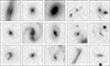 |
Fig. A.3. Example of MIR AGN with fPSF < 0.1. These images correspond to a physical size of around 25 kpc and are displayed with an inverse arcsinh scaling. |
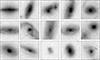 |
Fig. A.4. Example of DESI spectroscopic AGN with fPSF < 0.1. These images correspond to a physical size of around 25 kpc and are displayed with an inverse arcsinh scaling. |
All Tables
Percentage of AGN from each selection method that we also identified as AGN using a cut on the PSF contribution fraction.
Best-fit parameters for the log10(LPSF/[erg s−1]) versus log10(M*/[M⊙]) linear relation, in different redshift bins.
All Figures
|
Fig. 1. Euclid VIS PSF. We stacked 500 random empirical PSFs and show the mean PSF (top panel), standard deviation (central panel), and the coefficient of variation (bottom panel), calculated pixel by pixel. The pixel resolution is 0 |
| In the text | |
|
Fig. 2. X-ray luminosity of the X-ray-detected Euclid sources as a function of redshift. In blue we show the sources detected in EROMAIN, and in yellow those detected in 4XMM and CSC2. The top histogram shows the redshift distributions of the different samples, and the right histogram shows the distributions in the X-ray luminosity. |
| In the text | |
|
Fig. 3. Example mock Euclid VIS images with varying levels of PSF contribution (fPSF) to the total flux. The images were generated to mimic Euclid observations and include realistic Euclid noise and background. Each row corresponds to a different galaxy, with increasing PSF contribution fractions from left to right, at different magnitudes. The images correspond to a physical size of around 25 kpc and are displayed with an inverse arcsinh scaling. The blue circles show an aperture of 0 |
| In the text | |
|
Fig. 4. Comparison between the injected PSF contribution fraction and the predicted contribution fraction from Zoobot on the test set across the whole redshift range (0.5 < z < 2). The diagonal line is the 1:1 relation. The top plot shows the mean difference and the standard deviation as a function of the injected PSF contribution fraction. The colour bar indicates the number of sources in each 2D bin. |
| In the text | |
|
Fig. 5. RMSE and average RAE as a function of the injected PSF contribution fraction (top left panel), redshift (top right), S/N (bottom left), and size (bottom right). The error bars show the 95% interval from bootstrapping. The insets show the distribution of each quantity. The grey area of the top left panel corresponds to the level of the intrinsic fractional variation (standard deviation divided by the mean), considering the spatial and temporal variations in the observed Euclid VIS PSF. |
| In the text | |
|
Fig. 6. Similar to Fig. 5, but for the outlier fraction, calculated as the fraction of galaxies with RAE > 50% or |
| In the text | |
|
Fig. 7. Distribution of fPSF for the whole Euclid stellar-mass-selected sample of galaxies with 0.5 < z < 2 and log10(M*/M⊙) > 9.8. The vertical dashed lines represent the two adopted thresholds above which we classify galaxies as AGN according to the DL model, for the purpose of comparing with other AGN-selection methods. |
| In the text | |
|
Fig. 8. Fraction of galaxies in bins of the predicted PSF contribution fraction in the AGN samples from different selections (X-ray detection, MIR colours, and optical spectroscopy) and the non-AGN sample (see text in Sect. 2.3). |
| In the text | |
|
Fig. 9. X-ray and bolometric luminosity relations. The top panel shows the AGN luminosity, LPSF, as a function of X-ray luminosity, LX, for the EROMAIn sample (blue circles) and the 4XMM&CSC2 sample (orange squares). The solid blue and orange lines represent the best linear fit to each sample, respectively, while the dotted purple line is the best fit to the whole X-ray sample. The bottom panel shows the overlapping fraction of AGN as a function of the adopted cut on the X-ray luminosity (for the X-ray sample) or the bolometric luminosity (for the DESI spectroscopic sample, in green). The solid lines show the overlapping fraction of AGN defined by fPSF > 0.2, while the dashed lines show the fraction if we select AGN as defined by fPSF > 0.1. |
| In the text | |
|
Fig. 10. 2D histogram of the AGN luminosity (luminosity in the IE filter multiplied by fPSF) versus stellar mass, in different redshift bins, for all galaxies in our mass-limited sample. The white stars show the mean value, and the error bars show the dispersion of the data. The colours of the 2D histogram show the number of points in each bin. |
| In the text | |
|
Fig. 11. 2D histogram of SFR versus stellar mass in different redshift bins. Each 2D bin is colour-coded by the median value of fPSF (left) or the median value of log10(LPSF) (right) of all galaxies from our mass-limited sample in that bin. The black lines show the Popesso et al. (2023) SFMS at the median redshift of the bin. Only bins with at least ten galaxies are plotted. |
| In the text | |
|
Fig. 12. Similar to Fig. 11, but colour-coded by the fraction of galaxies with fPSF > 0.2 (top), fPSF > 0.4 (centre), and fPSF > 0.6 (bottom). |
| In the text | |
|
Fig. A.1. Normalised distribution of stellar mass (top left), redshift (top right), magnitude (bottom left), and total luminosity (bottom right) for the different types of AGN. |
| In the text | |
|
Fig. A.2. Example of X-ray AGN with fPSF < 0.1. These images correspond to a physical size of around 25 kpc and are displayed with an inverse arcsinh scaling. |
| In the text | |
|
Fig. A.3. Example of MIR AGN with fPSF < 0.1. These images correspond to a physical size of around 25 kpc and are displayed with an inverse arcsinh scaling. |
| In the text | |
|
Fig. A.4. Example of DESI spectroscopic AGN with fPSF < 0.1. These images correspond to a physical size of around 25 kpc and are displayed with an inverse arcsinh scaling. |
| In the text | |
Current usage metrics show cumulative count of Article Views (full-text article views including HTML views, PDF and ePub downloads, according to the available data) and Abstracts Views on Vision4Press platform.
Data correspond to usage on the plateform after 2015. The current usage metrics is available 48-96 hours after online publication and is updated daily on week days.
Initial download of the metrics may take a while.