


| Issue |
A&A
Volume 710, June 2026
|
|
|---|---|---|
| Article Number | A175 | |
| Number of page(s) | 13 | |
| Section | The Sun and the Heliosphere | |
| DOI | https://doi.org/10.1051/0004-6361/202660067 | |
| Published online | 16 June 2026 | |
Chromosphere of the quiet Sun
II. Atmospheric response to small-scale magnetic flux emergence
1
Rosseland Centre for Solar Physics, University of Oslo, P.O. Box 1029 Blindern, Oslo, NO-0315, Norway
2
Centre for Mathematical Plasma-Astrophysics, Department of Mathematics, KU Leuven, Celestijnenlaan 200B, 3001, Leuven, Belgium
3
Institute of Theoretical Astrophysics, University of Oslo, P.O. Box 1029, Blindern, Oslo, NO-0315, Norway
4
Sorbonne Université, Observatoire de Paris – PSL, École Polytechnique, Institut Polytechnique de Paris, CNRS, Laboratoire de Physique des Plasmas (LPP), 4 Place Jussieu, 75005, Paris, France
★ Corresponding author: This email address is being protected from spambots. You need JavaScript enabled to view it.
Received:
25
March
2026
Accepted:
2
May
2026
Abstract
Context. The couplings between the photosphere, chromosphere, and corona in the quiet Sun (QS) are governed by a complex interplay between magnetic structuring, heating, mass-loading, and radiative cooling. The current constraints on how this balance responds to variations in small-scale magnetic flux are limited.
Aims. We investigate how chromospheric heating and the thermodynamic response of higher atmospheric layers vary as a function of small-scale magnetic flux emergence under QS conditions.
Methods. We performed a parametric set of 3D radiative-MHD simulations with the Bifrost code, starting from a weakly magnetised quiet-Sun reference model and injecting horizontal magnetic flux of increasing amplitude into the sub-surface convection zone. We analysed the resulting chromospheric dynamics, heating, mass-loading, and coronal response in quasi-static regimes.
Results. Chromospheric temperatures and mechanical heating rise monotonically with increasing magnetic-field strength. Although the fractional contribution of shocks decreases from 23 to 5%, reconnecting current sheets (CSs) continue to remain steady at about 50%. In contrast, the temperature at the base of the corona exhibits a non-monotonic response, reaching a maximum at intermediate magnetic amplitudes and decreasing for the strongest-field case. We show that stronger magnetic-field strength increases chromospheric heating, thereby increasing the coronal-base density through efficient mass-loading, and amplifies radiative losses. These density-driven radiative losses dominate the coronal energy balance and, thus, lead to reduced coronal-base temperatures despite increased heating.
Conclusions. Our results demonstrate the sensitivity of chromospheric structure and dynamics to small-scale flux emergence and its key role in regulating coronal thermodynamics. In particular, this study has revealed a non-monotonic thermodynamic response in the upper atmosphere: stronger heating in the chromosphere can paradoxically lead to lower coronal temperatures as increased mass-loading enhances radiative losses. This result illustrates the chromosphere’s role as a thermodynamic gatekeeper, warranting further investigations of realistic flux-emergence models, as well as surface-to-corona parametrisation across various magnetic configurations, relevant to global solar wind models and space weather forecasts.
Key words: magnetic reconnection / magnetohydrodynamics (MHD) / radiation: dynamics / shock waves / Sun: atmosphere / Sun: chromosphere
© The Authors 2026
 Open Access article, published by EDP Sciences, under the terms of the Creative Commons Attribution License (https://creativecommons.org/licenses/by/4.0), which permits unrestricted use, distribution, and reproduction in any medium, provided the original work is properly cited.
This article is published in open access under the Subscribe to Open model. This email address is being protected from spambots. You need JavaScript enabled to view it. to support open access publication.
1. Introduction
The quiet Sun (QS) comprises most of the solar surface and exhibits a variety of small-scale magnetic structures. These are typically classified as network (a supergranular-spaced reticulum of strong kilogauss fields) or internetwork (i.e. a dense collection of weaker flux concentrations in between, see Bellot Rubio & Orozco Suárez 2019 for a review). This magnetic field is sustained via ubiquitous and ephemeral flux emergence, resulting from the solar dynamo (Schrijver et al. 1997; Martínez González & Bellot Rubio 2009; Díaz-Castillo et al. 2025).
Magnetic fields at the solar surface are commonly inferred via the Zeeman and Hanle effects. Recent advances have improved the reliability of photospheric line-of-sight magnetic field measurements at the disk centre with high-spatial-resolution instruments (e.g. Sinjan et al. 2024; Nóbrega-Siverio et al. 2024). However, retrieving other components of the magnetic field, especially in higher atmospheric layers, remains a significant challenge. In particular, the inversion of magnetic fields in the chromosphere is still highly uncertain due to line-formation complexities and limited diagnostics (e.g. De La Cruz Rodríguez & Van Noort 2017).
In numerical models, the magnetic field amplitude and topology are generally imposed as free parameters (Carlsson et al. 2019). This is critical, as the magnetic field configuration influences the chromospheric dynamics (e.g. Nindos et al. 2022), as well as its coupling with other layers of the atmosphere and, therefore, the way in which mass and energy are transferred to the solar environment. While several studies have started to explore the impact of various magnetic topologies on the chromosphere (Carlsson et al. 2016; Martínez-Sykora et al. 2019; Przybylski et al. 2022; Martínez-Sykora et al. 2023; Przybylski et al. 2025) as well as active-Sun amplitude flux-emergence (Archontis & Hansteen 2014; Ortiz et al. 2014; Hansteen et al. 2017, 2019), parametric investigations are still pending for QS conditions.
It has been recurrently shown that the coupling between the solar chromosphere and corona is governed by a delicate balance between heating, mass-loading, and cooling (Gudiksen & Nordlund 2005b; Rempel 2017; Carlsson et al. 2019). The coronal temperature alone provides an incomplete measure of the energy budget, and atmospheric coupling must therefore be understood as a joint mass–energy problem. This type of a non-linear feedback loop depends on magnetic geometry and therefore needs to be explored across the diverse configurations present on the Sun.
Magnetic fields are known to modulate chromospheric heating. Observations suggest that acoustic shocks alone might suffice to balance radiative losses in the lower chromosphere of some internetwork regions. However, their contribution likely drops to 30−50% near plage boundaries (Abbasvand et al. 2020b), showing that the magnetic field likely regulates the relative weight of heating mechanisms, which remains to be quantified (Carlsson et al. 2019). In Noraz et al. (2026, hereafter Paper I), we quantified the respective contributions of shock waves and current sheets (CSs) in a Bifrost QS simulation and found that they jointly provide the strongest contribution of the chromospheric heating for a weakly magnetised quiet-Sun simulation (see also Udnæs & Pereira 2025; Cherry et al. 2026 for complementary analysis on similar models). However, understanding how this chromospheric small-scale dynamics and subsequent energy deposition is evolving as a function of the magnetic-field topology and amplitude is still pending.
There is now a broad consensus that heating in the lower solar atmosphere is an intermittent, multi-physics process that can hardly be captured without comprehensive 3D radiative-MHD models (see e.g. Carlsson et al. 2019; Przybylski et al. 2025; Lamarre et al. 2025; Paper I). Such models can indeed provide essential constraints for parameterising this dynamics and subsequent mass-energy transfers in global approaches that employ crude chromospheric prescriptions. In particular, while modelling the chromosphere comprehensively will likely remain out of Space-Weather operational reach for the near future (see e.g. Brchnelova et al. 2023), improving the parameterisation of the low solar atmospheric coupling in different magnetic environments is both feasible and increasingly necessary (e.g. Van Der Holst et al. 2014; Parenti et al. 2022; Brchnelova et al. 2025; Wang et al. 2026).
Building on the work we presented in Paper I, we have extended it to a controlled parametric exploration to assess how the chromospheric thermodynamics varies under different QS conditions. Specifically, we aim to mimic idealised small-scale flux emergence with different amplitudes, and explore how the flux injected influences (i) chromospheric heating processes and (ii) the subsequent response of higher layers due to changes in mass and energy transfer.
In Sect. 2, we present the simulation setup. The behaviour of the flux we inject is described, along with the global impact on the magnetic and temperature structure. We then focus our analysis on changes in the chromospheric heating and dynamics in Sect. 3, before focussing on the coupling to higher layers in Sect. 4, where we investigate the changes in temperature and mass-loading. Finally, we discuss the different caveats of our models in Sect. 5 before presenting our conclusions in Sect. 6 and opening up the potential impact and perspective offered by these results.
2. Parametric setup of the experiment
2.1. Construction of the models
We used the ch012023 simulation (hereafter Ref) presented in Paper I as the reference run of our controlled parametric exploration. We solved the 3D time-dependent, resistive MHD equations with the Bifrost code (Gudiksen et al. 2011), which models the solar atmosphere from the sub-surface convection zone (CZ) to the low corona, including the photosphere, chromosphere, and transition region (TR), in a Cartesian box. This reference run reproduces QS conditions with an open magnetic topology characteristic of a coronal hole and self-consistently sustained by a local dynamo in the CZ (i.e. no magnetic flux is injected through the boundaries).
To mimic different idealised and small-scale flux-emergence configurations in the QS, we duplicated this reference run into two additional simulations, ch012023_by200 and ch012023_by800, in which a uniform horizontal magnetic-flux sheet (By = 200 and 800 G, respectively) is injected into convective upflows through the bottom boundary. These values were chosen to ensure efficient emergence through the convection zone, while spanning average photospheric fields, characteristic from weak to strong flux emergence under quiet-Sun conditions (see Sect. 2.3). All three runs share the same numerical setup, which we briefly summarise here (see Paper I for more details).
The simulations were computed on a 5123 grid spanning 12 Mm in both horizontal directions, with periodic boundary conditions and a constant horizontal resolution of 23 km (prefix ch012023). Vertically, the domain extends from 2.5 Mm below to 8 Mm above the mean solar surface (τ500 = 1) with non-uniform spacing: 30 km at the base of the CZ, 14−12 km in the photosphere and chromosphere, then up to 70.5 km at the coronal top. The lower boundary allows for inflows with entropy adjusted to maintain an effective temperature close to ∼5780 K, while the upper boundary applies an open characteristic-boundary scheme (Gudiksen et al. 2011, see also Tarr et al. 2024). In ch012023_by200 and ch012023_by800 (hereafter referred to as By200 and By800, respectively), the magnetic-flux sheet injection begins at t = 140 min, and continues for the remainder of the simulated time.
2.2. Behavior of the flux emergence
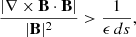
Magnetic flux is continuously injected from the bottom boundary, leading to a temporal evolution of the magnetic topology in the atmosphere above. To illustrate the morphological evolution, Fig. 1 shows the By800 model at three representative timesteps t0, t1, and t2 (see also Fig. 2). The normalised parallel current,
 (1)
(1)
 |
Fig. 1. Magnetic-field evolution during the three main phases of the By800 experiment for t0 = 140 min, t1 = 233 min and t2 = 325 min. The panels show the normalised parallel current, |∇×B ⋅ B|/|B|2 (grayscale), and the reconnecting current sheets (CSs; green), identified using the criterion of Eq. (1). Magnetic-field lines are shown with yellow streamlines, and the β = 1 surface is drawn with a dashed red line. We note how the height of the latter has moved from the initial t0 to the quasi-static timestep t2, due to the injection of emerging magnetic-loop structures, increasing the volume filled by a subsequently reconnecting CS. The associated movie is available online. |
with ϵ = 6 and ds = max(dx, dy, dz), is used to identify reconnecting CSs following the method of Paper I.
In the initial state (t0; left panel), the field is predominantly vertical (yellow lines), consistently with the imposed average vertical flux of 2.5 G, representative of quiet-Sun coronal-hole conditions (Harvey et al. 1982; Zwaan 1987). This experiment is initialised from the Ref model, whose detailed dynamics are discussed extensively in Paper I. Most CSs (green patches) are concentrated below the β = 1 surface (dashed red line), horizontally aligned in the photosphere and following the convective flows dynamics in the CZ.
During what we will refer to as the ‘transient phase’, horizontal magnetic flux is advected upwards from the lower boundary and begins to emerge into the chromosphere. At t1, in the middle panel, a dome-shaped structure between 4 < y < 8 Mm forms as the field rises, bounded by reconnecting CSs (green) that develop at the interface, due to interaction of the emerging field with the ambient one (see the corresponding animation, and also e.g. Archontis & Hansteen 2014; Ortiz et al. 2014). In the CZ, we note large areas (i.e. of a few Mm) where CSs are now absent and the normalised current is weak (darker regions). These correspond to upflows, where the uniform and untwisted horizontal flux is injected, as can be seen in the animation. Furthermore, the amplitude of the magnetic field injected at z = −2.5 Mm (By = 800 G in this case) is strong enough so that the CS formation is notably limited up to the photosphere, in comparison to the initial state, due to the subsequent increase in the Lorentz force. This leads to a preferential location of CSs in downflow lanes, where the kinetic energy density is stronger.
Once the emerging flux reaches the top of the domain and starts to leave through the open boundary conditions, a quasi-equilibrium settles as magnetic flux now both enters and leaves the domain, from the bottom and top boundaries, respectively. During this ‘quasi-static’ phase (t2; right panel), the injected flux has now spread in the whole domain, notably producing a substantial horizontal magnetic component, extending in the chromosphere and up to the top of the domain (see Fig. 1). The β = 1 surface has moved downwards as the magnetic pressure increased, while the volume occupied by CSs has expanded. This behaviour is further quantified in Sect. 3.2.
To further quantify the temporal evolution, we compute and illustrate in Fig. 2 the spatial average of the Alfvèn speed 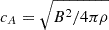 from 5 to 7 Mm above the photosphere. First, a pronounced decrease in cA is observed in both By200 (red) and By800 (green) starting at t ∼ 245 and 225 min, respectively. This marks the onset of magnetic flux emergence into the averaged volume. The decrease in cA further indicates that the density, ρ, increases faster than B2 on average. This shows that denser material is loaded up as the magnetic structures we inject rise into the atmosphere, which will be further analysed in Sect. 4. The earlier Alfvén speed decrease in the By800 case is then consistent with its stronger imposed field, and the corresponding increase in magnetic buoyancy, Fb. To first order, Fb scales with the field amplitude as Fb = gδρ/ρ ∝ β−1, where g, ρ, and β are the gravitational acceleration, density, and plasma-β parameter, respectively (Moreno-Insertis 1986; Cheung & Isobe 2014).
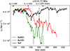 |
Fig. 2. Temporal evolution of the Alfvèn speed |
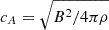
Once the magnetic flux begins to both enter and leave the mean volume continuously, the injected field has reached the upper part of the domain and the system enters the quasi-static phase in which the decrease in the Alfvén speed starts to saturate. This occurs from t ∼ 300 and 260 min in By200 and By800, respectively. The vertical dashed lines in Fig. 2 mark the one-hour segments within this phase that are used for the time-averaged analysis presented in the next sections.
2.3. Relaxed structure
We present in Fig. 3 a 3D rendering of the three runs at t2 = 325 min, namely, three solar hours after we started the flux-emergence experiment in both By200, and By800. This allowed us to compare their respective magnetic and thermal configurations during the quasi-static phase (time ranges between dotted lines of Fig. 1).
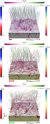 |
Fig. 3. 3D visualisations of magnetic and thermodynamic structures in the three simulations: Ref (top), By200 (middle), and By800 (bottom), shown during their quasi-static phases at t = 324 min. The corrugated horizontal surface marks the τ500 = 1 layer, coloured by the vertical magnetic field Bz. The vertical side panels show the convective velocity vz in the upper convection zone, while magnetic field lines, seeded from a uniform 15 × 15 grid at z = 3 Mm, are coloured by temperature. This transitions from pink in the chromospheric temperature minimum (∼4000 K), to white in the TR (∼40 000 K), and green in the low corona (∼500 000 K). The panels illustrate the progressive emergence of horizontal flux, from the nearly vertical, coronal-hole-like topology of Ref, through loop-dominated By200, to the strongly inclined, horizontally dominated configuration of By800. Associated movies are available online. |
We first note the Ref run exhibits a predominantly vertical topology consistent with quiet coronal-hole conditions analysed in Paper I and used as initial condition for By200 and By800. In contrast, the By200 and By800 cases display progressively more inclined ambient fields and an extended magnetic-loops network, reaching up to 5 Mm.
We select a solar-hour period over which we will perform temporally averaged analysis (see Fig. 2). We select this period from t = 301 to 361 min for both Ref and By200 runs, while we select this period from t = 266 to 325 min in By800 (see the dashed lines in Fig. 2). The corresponding mean unsigned photospheric field strengths are ⟨|Bz|⟩ = 21, 61, and 89 G for the Ref, By200, and By800 cases, respectively, once averaged over the solar hour over the τ500 nm = 1 surface. The three runs presented in this paper hence span different QS typical configurations, from weakly magnetised quiet-Sun conditions to strong small-scale emergence episodes (Bellot Rubio & Orozco Suárez 2019; Gošić et al. 2025).
Besides the expected change in topology, we also note the temperature structure changes between the cases as well. While Ref and By200 show coronal temperatures exceeding 100 kK (green shades), By800 regularly exhibits cooler temperatures in these upper layers (pink tones). This indicates a substantial modification of the thermal structure as well.
To quantify this change, we present the different temperature profiles of our models in Fig. 4. We first note that the intermediate By200 case (red) is consistently hotter than the Ref one (dark) at all heights, from the bottom of the chromosphere and above. However, this is not the case of the strong By800 run (green), which exhibits the hottest chromosphere, but also the coolest averaged temperature at the base of the corona. In the following, we aim to understand these different behaviours, first focussing on the chromosphere in Sect. 3 and its coupling with higher layers in Sect. 4.
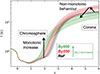 |
Fig. 4. Comparison of the temperature profiles as a function of height, among Ref, By200 and By800 in black, red and green, respectively. These vertical profiles, and the ones from the following figures, are averaged over one hour of solar time, illustrated in Fig. 2. Horizontal and temporal averages are illustrated with dotted lines, while the envelope indicates ±1 standard deviation in time. We use black arrows to underline the different noteworthy behaviours here; namely, the chromospheric temperature increase as a function of the magnetic amplitude we inject, along with a non-monotonic response at the base of the corona. |
We also see that the TR, defined here on this plot as the region between both chromospheric and coronal temperature plateaus, is wider as we increase the magnetic flux amplitude we inject. However, we ought to remain careful when horizontally averaging a corrugated surface such as the TR (see also Paper I) and we further note that we scarcely end up reaching a so-called flat coronal plateau in both the By200 (red) and By800 (green) cases. This visual TR broadening in height acknowledges the change in magnetic topology we see in Fig. 3. Indeed, the quasi-uniform vertical topology of Ref leads to similar TR heights over the horizontal extent of the box and, hence, a thinner averaged TR, while By800 exhibits a network of magnetic loops and concentrations, subsequently corrugating the TR over a broader range of heights (see e.g. Gabriel 1976).
3. Chromospheric heating
3.1. Impact on the mechanical heating
Fig. 5 shows vertical chromospheric profiles of the mechanical heating Qmech = Qν + Qη + Qcomp, where Qcomp is the positive compression contribution from the compressible term Qp∇v = −p∇ ⋅ v, Qν the viscous heating, and Qη the ohmic heating. All simulations exhibit a steep decrease in Qmech with height, due to the steep stratification in this region.
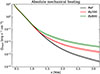 |
Fig. 5. Comparison of the mechanical heating profiles Qmech = Qν + Qη + Qcomp as a function of height, among Ref, By200, and By800 in black, red, and green, respectively, averaged horizontally in space and over one solar hour in time. The envelope indicates ±1 standard deviation in time during the solar-hour average. |
Yet the runs with larger injected By (By200 and By800) show a clear and systematic enhancement of the heating above z ∼ 1 Mm. The difference becomes increasingly pronounced as we go higher in the chromosphere, where the magnetic field is more dominant. This trend suggest that magnetic structuring regulates how mechanical energy is converted into heat and it is consistent with the observational picture where upper-chromospheric temperatures rise with magnetic strength (see e.g. Withbroe & Noyes 1977; Fröhlich & Lean 2004; Abbasvand et al. 2020a). Indeed, the profiles point to a more efficient heating as the amplitude of the chromospheric magnetic field increase and we now aim to investigate which processes are at the origin of such behaviour in our set of simulations.
3.2. Shocks and current sheets individual contributions
3.2.1. Tracking
Chromospheric temperatures and dynamics are sustained by a combination of upwardly propagating acoustic waves (Biermann & ten Bruggencate 1947; Schwarzschild 1948; Schmieder 1979), magneto-acoustic waves, Alfvén waves (Jess et al. 2015), and magnetic reconnection triggered by footpoint shuffling from convective motions (Parker 1972, 1983; Cargill 1993). These processes have been described in detail in the works of Gudiksen & Nordlund (2005a), Carlsson et al. (2016, 2019), Hansteen et al. (2015), Hansteen et al. (2019), Finley et al. (2022), Przybylski et al. (2022).
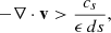
In high-Reynolds and high-Lundquist-number regimes such as the solar chromosphere, these processes are further expected to drive heating at small scales, such as strong velocity ∇ ⋅ v and magnetic field ∇ × B gradients, manifesting as shocks and reconnecting CSs, respectively. Following the methodology presented in Paper I, we detected shocks and CSs according to the sonic-compression,
 (2)
(2)
and normalised-parallel-current criteria presented in Eq. (1). cs is the sound speed, ϵ = 6 is tuned to strictly isolate nonlinear dissipation (e.g. shocks) from linear wave propagation (see Paper I for further details on the calibration).
Figure 6 summarises how shocks, CSs, and their associated mean mechanical heating respond to the imposed horizontal field. The left panels show the vertical evolution of their filling factors, defined as the fractional number of grid cells labelled as shocks. The middle panels display the mean mechanical heating ⟨Qmech⟩x locally for each process x = {sh, cs}, namely, averaged over cells labelled as shocks or CSs only, respectively. Finally, the right column illustrates the corresponding absolute contribution over the whole horizontal extent, which corresponds to the product of ⟨Qmech⟩x with the corresponding filling factor.
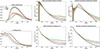 |
Fig. 6. Shock and CS thermodynamics. Comparison of different profiles as a function of height, among Ref, By200, and By800 in black, red, and green, respectively, averaged horizontally in space and over one solar hour in time. The left and middle columns illustrate the filling factors and the mean local mechanical heating at the process location, respectively. The right column panels illustrate the absolute contribution of these processes over the whole horizontal extent, corresponding to the product of the mean local contribution ⟨Qmech⟩x with the corresponding filling factor. Top and bottom rows present it for shocks and CSs, respectively. The envelope indicates ±1 standard deviation in time. |
3.2.2. Shocks
In the top-left panel, all simulations show shock formation starting at z ≃ 0.5 Mm, as expected from shock formation in the low solar atmosphere. At this height, all runs still exhibit a high-beta regime, so we do not expect a substantial change in the filling factor as a function of the amplitude of the magnetic field, as the latter is not dynamically dominant yet. We refer to Paper I for the dedicated analysis of the evolution with height and set our focus here on its consistent decrease in the chromosphere (0.5 ≲ z ≲ 2.5 Mm) as the injected By increases between the different runs. Several mechanisms likely contribute. First, the Lorentz force increasingly counteracts the steepening of upwardly propagating compressive fronts, which reduces shock formation from a dynamical standpoint. Second, the higher chromospheric temperatures in the magnetised runs raise the sound speed cs ∝ T1/2, making it more difficult for waves to reach the supersonic regime required for shocks. Third, the magnetic structure of the chromosphere changes (see Fig. 3), and more especially the plasma-β = 1 surface is pushed downwards as the magnetic field amplitude increases. This causes the acoustic–magnetic mode conversion to occur earlier during the ascent of wave packets. More wave energy is therefore converted into the fast magnetic mode, which shocks less readily because the Alfvén speed increases. Fourth, we can also mention the deflection of slow-mode acoustic waves by coherent loop structures present in By200 and By800, as the top of which now reaches low-beta regime heights (see also Sect. 3.3). This effect will be enhanced as β is lower, hence, as the amplitude of the magnetic field is stronger. Determining the relative influence of these processes will require a dedicated analysis, which has been left for future work (see also Udnæs & Pereira 2025; Enerhaug et al. 2025; Cherry et al. 2026).
In the top-middle panel of Fig. 6, we examine the evolution of the mean shock-associated heating, ⟨Qmech⟩sh. We find that it initially decreases in the lower atmosphere (z < 0.5 Mm) as By increases. Because this quantity is restricted to shocked cells, this trend does not reflect changes in the filling factor, but instead indicates a local reduction in shock intensity during their formation. Force-balance diagnostics show that the Lorentz force becomes the dominant counteracting term along the propagation direction at these heights, partially inhibiting front steepening in the early stages of shock development.
At greater heights, this trend reverses. Although shocks are less frequent in the By800 case, those that do form release significantly more mechanical energy once they reach z ≳ 1 Mm, and ⟨Qmech⟩sh increases with By. This behaviour becomes even more apparent when considering the absolute contribution of shocks in the top-right panel. The decrease in shock filling factor with increasing By leads to a reduction in their total contribution to Qmech in the lower chromosphere (0.5 ≲ z ≲ 1.5 Mm).
However, in the upper chromosphere (1.5 ≲ z ≲ 2.5 Mm), the absolute contribution increases despite the reduced filling factor. This implies that the rise in ⟨Qmech⟩sh more than compensates for the smaller spatial coverage of shocks. This behaviour cannot be attributed solely to a selection effect. The increase in the absolute shock contribution demonstrates that shock-related dissipation becomes intrinsically stronger at larger By, even when integrated over the full horizontal extent. This points to stronger and/or more dissipative perturbations in the upper chromosphere, consistent with magnetic modification of wave propagation, channelling, and mode coupling in the low-β regime we previously discussed, leading to fewer but more energetic magneto-acoustic shocks.
3.2.3. Current sheets
Despite the overall decrease in the CS filling factor with height as the plasma β decreases below 1, we note two different regimes when it comes to comparing the different simulations and thus the impact of the injected By in the bottom-left panel. As the latter increases, the filling factor first diminishes in most of the chromosphere (z ≲ 2 Mm) before starting to increase higher up. The overall reduction of β throughout the low-chromospheric layers of By200 (red) and By800 (green) strengthens the retro-action of the Lorentz-force on plasma flows, making the field less susceptible to twisting and therefore less prone to forming new small-scale CSs. Nevertheless, the trend reversal at higher altitude (z ≳ 2 Mm) acknowledges the particularity of By200 and By800 quasi-static regimes. In those, the accumulated horizontal field, loaded by flux emergence, forms a dynamic network of low-lying loops that have been randomly shuffled on the way, which will further promote non-parallel interaction with the newly emerging flux. These interactions produce extended current layers and long-lived reconnection sites, consistent with earlier studies of chromospheric reconnection and flux emergence-driven CSs (Archontis & Hansteen 2014; Hansteen et al. 2017, 2019; Robinson et al. 2022).
When looking at the mean mechanical heating associated with reconnecting CS events ⟨Qmech⟩cs in the bottom-middle panel, this increases consistently across the chromosphere as a function of the injected By. This is further pronounced as the β ≳ 1 regime is reached. Even though we have seen reconnection sites become less common below z ∼ 2 Mm, their local heating rate does indeed grow substantially in this regime. The decrease in β ∝ eint/emag enhances the magnetic energy density, emag, relative to the internal energy, eint, which favours strong transfer via ohmic dissipation. Flux emergence further drives reconnection by forcing interactions between the rising field and the pre-existing chromospheric network, which not only increases ohmic heating, but also compressive and viscous contributions generated by reconnection outflows (see also Paper I). Together, these effects lead to a robust enhancement of reconnecting-CS-driven mechanical heating across the upper chromosphere, as further confirmed by the evolution of their absolute contribution to Qmech in the bottom-right panel.
3.3. Small-scale dynamics changes
To illustrate how enhanced magnetic fields modify chromospheric small-scale dynamics, Fig. 7 shows temperature maps at three representative heights in the By800 model, namely z = 0.5, 1.0, and 1.5 Mm (left to right). Only one quarter of the horizontal domain is displayed to emphasise fine-scale structuring. Shocks (purple) and CSs (green), are overlaid on greyscale temperature maps, where brighter regions correspond to hotter plasma. We will discuss it in direct comparison with the Ref case, for which we refer the interested reader to Paper I for details.
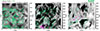 |
Fig. 7. Shocks (purple) and CSs (green) interplay with temperature structures (greyscale) in the chromosphere of By800. A zoom-in on a 6 × 6 Mm2 area is proposed to focus on small-scale dynamics. Shock and CS overlays are only considered on a 5 × 5 Mm2 portion, to further illustrate the overlap between them and temperature structures. The ϵ value specified here refers to the calibration of shocks and CS detections presented in Paper I. The associated movie is available online. |
At z = 0.5 Mm, the thermal morphology remains broadly similar to the reference case. CSs are already present but shocks are rare due to the relatively low average Mach number at this height (see also Fig. 6). CSs are preferentially spreading horizontally at this height due to the convective overturn and produce relatively thick overlays here, even though the underlying structures remain intrinsically thin (e.g. Paper I, see also Eq. 1).
At z = 1.0 Mm, shocks become clearly visible, although their filling factor remains limited in comparison to Ref, as can be expected from the top-left panel in Fig. 6. They correlate well with local temperature enhancements, confirming their role in intermittent small-scale heating already discussed in Paper I. However, a key difference is that CSs now also coincide with hot (brighter) regions at this height, which was only observed higher in the atmosphere of Ref. In By800, the horizontally averaged plasma-β is systematically reduced throughout the chromosphere, so that magnetic energy is comparable to internal energy (β ∼ 1) already at z ∼ 1 Mm. As a result, ohmic dissipation associated with CSs is no longer energetically constrained (i.e. emag ≳ eint) and can visibly imprint the local temperature structure.
At z = 1.5 Mm, the dynamics become strongly magnetically organised. The temperature and dissipation patterns are elongated predominantly along the y-direction, reflecting the imposed strong By = 800 G at the lower boundary of the domain. This large-scale magnetic configuration now visibly channels shock propagation (see animation attached to Fig. 7) and reshapes the flow morphology through Lorentz-force feedback. The average plasma-β at this height is about an order of magnitude smaller than in Ref, reaching about 0.1 on average, which explains the dominant magnetic control of the chromospheric structuring.
3.4. Summary of the contributions
To give an overall summary of the different contributions to the mechanical heating over the whole chromosphere, we define the chromospheric boundaries following the approach proposed in Paper I. The bottom height is set by reporting where the photospheric radiative equilibrium approximation breaks (Schwarzschild 1906), which occurs, in practice, at z = 600, 570, and 530 km in Ref, By200, and By800, respectively. The top of the chromosphere is subsequently approximated where the horizontally averaged temperature reaches 20 kK, following the common proxy for the substantial decrease in Hα emissions. This is met at z = 2.57, 2.35, and 2.11 Mm. We further discuss this later change and its implications in Sect. 4.
As already presented for Ref in Paper I, we integrated the relevant mechanical heating terms Qmech = Qν + Qη + Qcomp over the defined chromospheric extent and show them in Fig. 8 for the different runs. The resulting energy budget is summarised as a pie chart, with the outer ring indicating the heating processes (shocks, CSs, or neither) and the inner ring specifying the deposition term contributions.
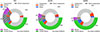 |
Fig. 8. Relative contributions of shocks (purple), CSs (green), and non-steep gradients (white) to the integrated mechanical heating of the chromosphere (Qmech = Qν + Qη + Qcomp, in red, blue, and grey, respectively). We present it for the three runs studied here: Ref (left), By200 (middle), and By800 (right). The different profiles used are spatially averaged over the chromospheric extent defined in the text body, with the outer ring indicating the physical processes involved (shocks, CSs, or neither), and the inner ring explicitly showing the associated dissipation mechanisms: viscous (red), ohmic (blue), and compression (grey). A darker shade of grey is used to highlight the shock compression contribution (see also Appendix A of Paper I). The hatched segments indicate the contribution of regions where both shocks and CSs overlap. |
The relative contribution of shocks (purple) to the mechanical heating decreases with increasing injected magnetic field strength, dropping from about one fourth in the weakly magnetised QS Ref case to about 5% in the strong By800 model. In contrast, heating associated with reconnecting CSs (green) consistently accounts for about half of the total budget (55 to 47%). Combined with the increase in total mechanical heating reported in Fig. 5, these results indicate that, although the filling factor of CSs decreases, their local heating efficiency increases substantially, as expected from the bottom-right panel of Fig. 6. This enhancement is primarily driven by the larger magnetic energy reservoir and its subsequent release through slow diffusion and reconnection-dynamics deposition within CSs, as illustrated further in Sect. 4.3. The substantial increase in the relative Ohmic heating (blue) in CSs contributions is also consistent with observational trends when going towards more-active regions (Morosin et al. 2022).
We can also note that the contribution of non-steep gradient (white part) increases as well from Ref to By800. This contribution likely comes from the energy deposition of broader current layers, but also the propagation of high-amplitude and linear waves (see the animation attached to Fig. 3 in Paper I). This is consistent with the scenario of an increased ramp effect, happening when the inclination of the field is more pronounced in the low solar atmosphere (Stangalini et al. 2011), subsequently allowing for a broader spectrum of waves to propagate in the upper atmosphere. A detailed characterisation of this transmission, and its quantitative impact on chromospheric and coronal coupling, lies beyond the scope of the present study (see e.g. Stangalini et al. 2025; Udnæs & Pereira 2025; Enerhaug et al. 2025; Cherry et al. 2026).
4. Atmospheric coupling
4.1. Increased density scale height
Understanding the non-monotonic behaviour of Tcor, bot(Bz), despite the monotonic increase in Tchromo(Bz), requires examining the coupling between the chromosphere and corona. To this end, and to elucidate the coronal temperature decrease in the By800 run observed in Fig. 4, we show horizontally and temporally averaged profiles of density and radiative cooling in Figs. 9 and 10, respectively. Both quantities increase consistently in amplitude at all heights as a function of the magnetic field amplitude injected (from black to green).
 |
Fig. 9. Comparison of density profiles among Ref, By200 and By800 in black, red, and green, respectively, averaged horizontally in space and over one solar hour in time. The envelope indicates ±1 standard deviation in time. |
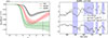 |
Fig. 10. Left: Comparison of radiative cooling profiles. The layout is similar to Fig. 9. Right: Temporal evolution of temperature T (solid), density ρ (dotted) and radiative cooling Q (dotted-dashed) values, averaged over the horizontal extent at z = 5 Mm. Blue-shaded time ranges highlight periods when the temperature decreases substantially, in order to compare with radiative cooling and density enhancements. |
In Fig. 9, the density profiles of By200 and By800 start to deviate from the Ref profile already in the upper chromosphere, around z ∼ 2 Mm, leading monotonically to denser plasma higher up in comparison to Ref. This deviation is accompanied by a change in the slope of the profiles, indicating a sudden increase in the density scale height, Hρ = Δz/Δlnρ. In the lower chromosphere (0.5 < z < 1.5 Mm), Hρ ∼ is consistent with 0.12 Mm for the 3 models, whereas the profiles become nearly flat above z ∼ 5 Mm, implying a scale height exceeding the vertical extent left up to the top of the simulated domain. We can understand this behaviour as Hρ ∝ T under hydrostatic approximation. Although the hydrostatic approximation may appear restrictive given the highly dynamic, small-scale nature of the simulations, it appears to remain consistent once quantities are averaged over space and time in the context of this work.
As a result, the onset of the chromospheric temperature rise leads, to first order, to an increase in Hρ and sets the thermodynamic conditions at the coronal base by increasing density. This highlights the importance of chromospheric structure, topology, and thermodynamics in energy and mass transport up to the lower solar corona.
4.2. Enhanced radiative cooling
In the left panel of Fig. 10, we show a comparison of the radiative cooling profiles Qrad. We include radiative losses occurring from the top of the chromosphere upwards; namely, those computed using the semi-empirical radiative-loss recipes of Carlsson & Leenaarts (2012) for hydrogen, calcium, and magnesium, together with optically thin radiative losses based on CHIANTI atomic data (Dere et al. 1997; Landi et al. 2006). Here, we express Qrad per unit mass, thereby limiting the dominance of high-density regions seen for By800. Figure 9 offers a meaningful comparison, along with a consideration of the possibility of erg/s/cm3 based on the plot.
Above z ∼ 1.5 Mm, the absolute amplitude of Qrad increases with the imposed magnetic-field strength. This behaviour is consistent with the enhanced density stratification discussed in the previous section, since under optically thin and fully ionised conditions, appropriate for the corona, radiative losses scale as Qrad ∝ ρ2 (e.g. Mihalas & Weibel-Mihalas 1984; Rutten 2003). The pronounced enhancement of radiative cooling in the By800 run relative to Ref is particularly noteworthy, given that presenting the losses per unit mass already mitigates the impact of the highest density regions.
To further demonstrate that the density increase, and the resulting enhancement of radiative cooling, is the primary driver of the temperature decrease observed at the coronal base in Fig. 4, we examine the temporal evolution of temperature, density, and radiative cooling in the right panel of Fig. 10, after a horizontal averaging at z = 5 Mm in the By800 simulation. Blue-shaded intervals indicate periods of pronounced temperature decrease. These episodes coincide with enhanced radiative cooling rates (dash-dotted curve) and periods of high or an increase in densities (dotted curve).
The correlations shown here are particularly relevant given that all quantities are averaged over the full horizontal extent of the domain. They reveal a clear causal imprint of density enhancements on radiative cooling, as expected, and well as, in turn, on the global temperature evolution at this height. It is important to recall that other non-local transport processes, such as thermal conduction and advection, can also contribute to coronal cooling at coronal heights. However, these processes fluctuate rapidly between heating and cooling and exhibit no clear temporal correlation with the mean temperature decreases, even when examined across multiple coronal heights.
Another aspect that can contribute to the non-monotonic coronal temperature response is the dominant orientation of the magnetic field, which varies from one model to another (see Fig. 3). A loss of magnetic connectivity to the lower atmosphere would modify the redistribution of heat. However, such a configuration should instead lead to higher coronal temperatures, as the deposited energy could no longer be efficiently transported downwards by thermal conduction, which was not observed for By800. Enhanced density-driven radiative losses therefore emerge as the dominant cooling mechanism governing the global temperature-decrease episodes and the reduced mean coronal-base temperature of By800 relative to Ref, as seen in Fig. 4.
4.3. Mass-loading
We have shown that the overall temperature decrease at the base of the corona in By800 relative to Ref is primarily driven and sustained by an increase in density at that height. This naturally raises the question of how mass is effectively transported from the chromosphere into the low corona. Addressing this question quantitatively is beyond the scope of the present paper; nonetheless, our aim here is to propose a qualitative analysis of the simulated dynamics to illustrate the mechanisms of low-atmospheric coupling and further guide the quantification of mass fluxes in future works.
In Fig. 11, we illustrate several diagnostic quantities that characterise and compare the plasma dynamics in the Ref (top row) and By800 (bottom row) cases. In the Ref simulation, we observe recurrent type-I spicule dynamics, characterised by upwards motions (see red arrow in the right panel) of dense (red patches in the left panel) and cool (blue patches in the middle panel) chromospheric plasma. The animation shows that these spicules are shock-driven and guided by the predominantly vertical magnetic field, in agreement with previous analyses of the same run (Fig. 4 of Noraz et al. 2026) and with observational interpretations (Hansteen et al. 2006; De Pontieu et al. 2007). We see in the left panel that this spicular dynamics largely contribute to chromosphere-to-corona mass-loading, together with magnetic swirling motions, as also illustrated in Fig. 1 of Noraz et al. (2026). Although a quantitative assessment of their respective contributions to mass and energy transport lies beyond the scope of this study, these processes are expected to play a key role in quiet-Sun atmospheric coupling (see e.g. Martínez-Sykora et al. 2017; Finley et al. 2022; Breu et al. 2023; Skirvin et al. 2024; Chandra et al. 2026). In particular, the role of spicules in this coupling remains under debate (Klimchuk 2015; Sow Mondal et al. 2022).
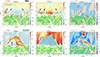 |
Fig. 11. Mass-loading behavior of Ref (top row) and By800 (bottom row). We highlight the position of shocks and CSs for all panels, following Eqs. (2) and (1), respectively. Left: Density variation, δρ/⟨ρ⟩x, y, taken at x = 6 Mm for each given time step and of each given simulation. This illustrates material more (red) or less (blue) dense than the surrounding material at that height. Middle: Same but for the temperature variation, δT/⟨T⟩x, y. Right: Same but for the vertical velocity component, vz, where red (blue, respectively) shows upwards (downwards, respectively) motions. Please note for the top row that dark arrows indicate over-densities, corresponding here to cooler material entering the coronal medium, and corresponding to shock-mediated (purple contours) type-I spicule dynamics (see also the red arrow indicating an upwards spicular motion and also see Fig. 4 of Paper I). We also note that for the bottom row, the dark arrow highlights the motion of the emerging magnetic loop-like structure, transporting the over-density (red) up to coronal heights. Interactions with the overlying magnetic field create thin reconnecting CS structure (green contours), where bipolar flows are highlighted by red and blue arrows (see also Fig. 5 of Paper I). Associated movies are available online. |
In contrast, the bottom row reveals a notably different magnetic and dynamical regime in By800. We recall here that δρ(y, z)/⟨ρ⟩(z) is the relative difference with respect to the horizontally averaged density at this height, z, and that this reference value has increased in By800 (see Fig. 9). The magnetic field now exhibits a strong horizontal component resulting from the imposed flux injection, as discussed in Sect. 2. At granular scales, this manifests as the emergence of low-lying magnetic loops (black arrow in the bottom-left panel). As these loops rise through the chromosphere, their upper segments trap and advect cool, dense chromospheric plasma upwards into the corona, as evidenced by the co-spatial red and blue patches in the bottom-left and bottom-middle panels, respectively (see the attached animation). This process contributes efficiently to increasing the density at the base of the corona, consistent with similar mechanisms identified in more magnetically active simulations (Druett et al. 2022).
We stress that the increase in horizontally averaged density in Fig. 9 reflects a combination of enhanced heating and direct mass injection associated with flux emergence, both contributing to the coronal mass-loading. To further assess this point, we analysed regions of By800 without flux emergence and still found enhanced heating and a systematic increase in column mass with respect to the reference case. This indicates that the density increase is not solely driven by the emergence-related structure, but that it also reflects a more broadly global thermodynamic response.
Finally, we can note from the animation that the top of the dome-like magnetic structure interacts continuously with the overlying magnetic field during its emergence. In the bottom-left panel, we indicate upwards and downwards plasma motion associated with the reconnecting structure, with a red and blue arrow, respectively. The corresponding thin green overlay between the ambient field and magnetic dome structure can track the core part of the CS that is dynamically relevant for reconnection (thanks to Eq. 2) where these bipolar flows originate. The upwards jet gives birth to a high-speed surge, as acknowledged by the red patch at the top of the right panel, between y = 6 and 8 Mm. This type of chain of events is recurrent in By800 and should be further characterised in future comparisons with observational constraints (see e.g. Heyvaerts et al. 1977; Yokoyama & Shibata 1995; Isobe et al. 2005, 2008; Nóbrega-Siverio et al. 2024; Huang et al. 2026).
5. Discussion
As illustrated by the animations associated with Figs. 3 and 11, small-scale flux-emergence events that transport chromospheric plasma to higher atmospheric layers appear to be a key mechanism for explaining the enhanced density at the base of the corona in By800. However, it should be noted that the global increase in temperature and the resulting modification of the pressure gradient across the horizontal extent of the domain might also contribute to driving this mass-loading. However, quantifying the relative contribution of these processes is beyond the scope of the present study and would require a dedicated analysis similar to that proposed by Druett et al. (2022).
The flux-emergence scenarios considered here are deliberately idealised, relying on the injection of untwisted horizontal magnetic fields at the lower boundary. While this approach is well-suited for controlled parametric exploration, future studies should aim to incorporate more realistic boundary conditions, either driven by observations (e.g. Chen 2025) or self-consistently coupled to global convection and dynamo models (e.g. Fang et al. 2012).
Because the magnetic flux is continuously injected, the system does not relax towards a passive post-emergence state but instead approaches a quasi-stationary, driven regime, in which heating, mass-loading, and radiative cooling reach a dynamic balance. Although a slow secular evolution remains visible (see Fig. 2), the main thermodynamic trends discussed here are established after the initial transient phase and remain robust, even at later stages of By200 simulated duration.
We want to stress here that the coronal temperatures obtained in this set of simulations should not be interpreted as definitive predictions. As demonstrated here, the coronal thermal structure strongly depends on how chromospheric heating and energy dissipation are modelled. Previous studies have shown that additional physical ingredients, such as ion–neutral interactions and non-equilibrium ionisation, can significantly modify chromospheric heating efficiencies and loop thermodynamics (Martínez-Sykora et al. 2012; Shelyag et al. 2016; Nóbrega-Siverio et al. 2020; Martínez-Sykora et al. 2020). These effects are available within Bifrost and should be explored in future extensions of the present work. Furthermore, coronal temperatures are also expected to depend on magnetic topology and spatial scale. Larger scale or more active configurations have been shown to produce hotter, million-degree coronae (Carlsson et al. 2016; Finley et al. 2022, see also the conclusion of Przybylski et al. 2025), underscoring the need to extend parametric studies to a broader range of magnetic environments.
We conservatively restricted our analysis to heights below 7 Mm. Above ∼7.5 Mm, the solution becomes increasingly sensitive to the top boundary condition. However, all trends discussed in this study, including the non-monotonic coronal response, are established well below this region and are not affected, either qualitatively or quantitatively, by measurable boundary effects in the analysis performed.
6. Conclusion and perspective
In this work, we conducted a parametric 3D radiative-MHD study of quiet-Sun atmospheric coupling with Bifrost, building on the reference simulation presented in Paper I. By injecting horizontal magnetic flux of increasing amplitude into the sub-surface convection zone, we constructed two additional models, spanning weakly magnetised, coronal-hole-like conditions (labelled Ref in the paper) to more typical QS amplitudes with intermediate and strong small-scale flux emergence (referred to as By200 and By800; Fig. 3). All the simulations reached a quasi-static state into which the magnetic flux both enters and leaves the computational domain, enabling a direct comparison of their thermodynamic and dynamical properties.
The chromosphere and corona respond differently to increasing magnetic-field amplitude. While the chromospheric temperature increases monotonically with the amplitude of the emerging flux imposed, the temperature at the base of the corona shows a non-monotonic response, first rising in the intermediate case relative to the reference case and then decreasing in the strongly magnetised case (see Fig. 4). This contrast motivated an analysis of chromospheric heating and atmospheric coupling.
In Sect. 3 we show that the total mechanical chromosheric heating increases with magnetic-field strength, driven primarily by reconnecting current sheets, which consistently contribute about half of the heating (55−47%). Although their filling factor decreases in most of the chromosphere, their local heating efficiency increases as additional magnetic energy is injected, due to the associated reduction in plasma-β. In contrast, shock-driven heating becomes progressively less important, from 23% in Ref to 5% in By800. Taken together, stronger magnetic fields promote more efficient chromospheric heating in our QS models.
Despite this enhanced heating, Sect. 4 shows that the coronal-base temperature decreases in the strongly magnetised case, due to a substantial density increase. Enhanced chromospheric heating increases the density scale height, thereby setting a higher density at the base of the corona, through the combined effect of both heating-induced and direct mass-loading from flux emergence. This density increase strongly amplifies radiative losses, which dominate the cooling in coronal energy balance and lead to global temperature-decrease episodes. The cooler coronal-base temperatures, observed in the strongly magnetised case, therefore do not reflect reduced heating efficiency, but a density-controlled equilibrium tightly linked to the redistribution of energy and mass across atmospheric layers.
These results highlight the central role of chromospheric temperature in setting the density scale height, which in turn constrains the density supplied to the corona and subsequent thermal equilibrium. Low atmospheric heating and mass-loading thus emerge as key regulators of coronal thermodynamics, even under increased magnetic activity. This has direct implications for surface-to-corona coupling in solar-wind models. While frameworks such as Wang–Sheeley–Arge relate surface magnetic fields to wind properties (Wang et al. 1990; Arge & Pizzo 2000; Arge et al. 2004), they still rely on simplified low-atmosphere parameterisations, despite a strong sensitivity to lower-boundary conditions (e.g. Kuźma et al. 2023). Our results indicate the need for an explicit incorporation of chromospheric heating and mass-loading in these parameterisations.
Figure 12 summarises the density at the top of the chromosphere and the temperature at the coronal base as functions of the mean unsigned photospheric field, ⟨|Bz|⟩photo. While ρtop, chromo increases monotonically with ⟨|Bz|⟩photo, Tbot, corona exhibits a non-monotonic response, with a maximum at intermediate field strength followed by a decline beyond a threshold value. We stress that the three simulations considered here do not constitute a dense parametric survey, but rather a controlled parametric exploration aimed at isolating the underlying physical mechanisms. Assessing the robustness and physical origin of this trend over a broader parameter space is a key objective of future work.
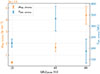 |
Fig. 12. Density at the top of the chromosphere, ρtop, chromo (orange symbols, left axis), and temperature at the base of the corona, Tbot, corona (blue symbols, right axis), as functions of the mean unsigned photospheric vertical magnetic field, ⟨|Bz|⟩photo. The chromospheric density is averaged at the height where the horizontally averaged temperature reaches 20 kK, while the coronal temperature is averaged at z = 6 Mm. Error bars indicate one standard deviation in time over the selected quasi-static interval. The figure highlights the monotonic increase in chromospheric density with magnetic-field strength and the non-monotonic response of the coronal-base temperature. |
The strong density-driven radiative cooling reported here also implies enhanced emission signatures potentially observable with the current instrumentation (e.g. Robinson & Carlsson 2023). Future comparisons with AIA and Solar Orbiter observations, as well as future facilities such as EST (Quintero Noda et al. 2022) and AtLAST (Wedemeyer et al. 2025) will help constrain chromospheric heating mechanisms and the mass–energy coupling between the lower solar atmosphere and the corona.
Data availability
Movies associated with Figs. 1, 3, 7 and 11 are available at https://www.aanda.org
Acknowledgments
All authors are thankful to F. Zang, N. Poirier, B. Gudiksen, V. Hansteen, J. Martínez-Sykora, K. Krikova and L. Rouppe van der Voort for useful discussions. The authors also thank the anonymous referee for useful and constructive remarks. We acknowledge funding support by the European Research Council (ERC) under the European Union’s Horizon 2020 research and innovation programme (grant agreement No 810218 WHOLESUN and No 101141362 Open SESAME), by the Research Council of Norway through its Centres of Excellence scheme (RoCS project number 262622), and through computational resources provided by Sigma2, the National Infrastructure for High Performance Computing and Data Storage in Norway. The work of GA was supported by the Action Thématique Soleil-Terre (ATST) of CNRS/INSU PN Astro, also funded by CNES, CEA, and ONERA. Data manipulation was performed using the numpy (Harris et al. 2020) and the in-house Bifrost analysis pipeline helita python packages. Figures in this work were produced using the python packages matplotlib (Hunter 2007) and pyvista (Sullivan & Kaszynski 2019).
References
- Abbasvand, V., Sobotka, M., Heinzel, P., et al. 2020a, ApJ, 890, 22 [Google Scholar]
- Abbasvand, V., Sobotka, M., Švanda, M., et al. 2020b, A&A, 642, A52 [EDP Sciences] [Google Scholar]
- Archontis, V., & Hansteen, V. 2014, ApJ, 788, L2 [NASA ADS] [CrossRef] [Google Scholar]
- Arge, C. N., & Pizzo, V. J. 2000, J. Geophys. Res.: Space Phys., 105, 10465 [NASA ADS] [CrossRef] [Google Scholar]
- Arge, C., Luhmann, J., Odstrcil, D., Schrijver, C., & Li, Y. 2004, J. Atmos. Solar-Terr. Phys., 66, 1295 [NASA ADS] [CrossRef] [Google Scholar]
- Bellot Rubio, L., & Orozco Suárez, D. 2019, Liv. Rev. Sol. Phys., 16, 1 [Google Scholar]
- Biermann, L., & ten Bruggencate, P. 1947, Veroeffentlichungen der Universitaets-Sternwarte zu Goettingen, 0005, 223 [Google Scholar]
- Brchnelova, M., Kuźma, B., Zhang, F., Lani, A., & Poedts, S. 2023, A&A, 678, A117 [NASA ADS] [CrossRef] [EDP Sciences] [Google Scholar]
- Brchnelova, M., Gudiksen, B., Carlsson, M., Lani, A., & Poedts, S. 2025, A&A, 693, A74 [NASA ADS] [CrossRef] [EDP Sciences] [Google Scholar]
- Breu, C., Peter, H., Cameron, R., & Solanki, S. K. 2023, A&A, 675, A94 [NASA ADS] [CrossRef] [EDP Sciences] [Google Scholar]
- Cargill, P. J. 1993, Sol. Phys., 147, 263 [Google Scholar]
- Carlsson, M., & Leenaarts, J. 2012, A&A, 539, A39 [NASA ADS] [CrossRef] [EDP Sciences] [Google Scholar]
- Carlsson, M., Hansteen, V. H., Gudiksen, B. V., Leenaarts, J., & De Pontieu, B. 2016, A&A, 585, A4 [NASA ADS] [CrossRef] [EDP Sciences] [Google Scholar]
- Carlsson, M., De Pontieu, B., & Hansteen, V. H. 2019, ARA&A, 57, 189 [Google Scholar]
- Chandra, S., Cameron, R., Przybylski, D., & Solanki, S. K. 2026, A&A, 706, A53 [NASA ADS] [CrossRef] [EDP Sciences] [Google Scholar]
- Chen, F. 2025, arXiv e-prints [arXiv:2511.02362] [Google Scholar]
- Cherry, G., Gudiksen, B., Finley, A. J., & Noraz, Q. 2026, A&A, 705, A42 [NASA ADS] [CrossRef] [EDP Sciences] [Google Scholar]
- Cheung, M. C. M., & Isobe, H. 2014, Liv. Rev. Sol. Phys., 11, 3 [Google Scholar]
- De La Cruz Rodríguez, J., & Van Noort, M. 2017, Space Sci. Rev., 210, 109 [CrossRef] [Google Scholar]
- De Pontieu, B., Hansteen, V. H., Rouppe Van Der Voort, L., Van Noort, M., & Carlsson, M. 2007, ApJ, 655, 624 [NASA ADS] [CrossRef] [Google Scholar]
- Dere, K. P., Landi, E., Mason, H. E., Monsignori Fossi, B. C., & Young, P. R. 1997, A&AS, 125, 149 [NASA ADS] [CrossRef] [EDP Sciences] [Google Scholar]
- Díaz-Castillo, S. M., Fischer, C. E., Moreno-Insertis, F., et al. 2025, A&A, 695, A45 [NASA ADS] [CrossRef] [EDP Sciences] [Google Scholar]
- Druett, M. K., Leenaarts, J., Carlsson, M., & Szydlarski, M. 2022, A&A, 665, A6 [NASA ADS] [CrossRef] [EDP Sciences] [Google Scholar]
- Enerhaug, E., Carlsson, M., Szydlarski, M., Gudiksen, B. V., & De Moortel, I. 2025, A&A, 701, A137 [NASA ADS] [CrossRef] [EDP Sciences] [Google Scholar]
- Fang, F., Manchester, W., Abbett, W. P., & Van Der Holst, B. 2012, ApJ, 745, 37 [Google Scholar]
- Finley, A. J., Brun, A. S., Carlsson, M., et al. 2022, A&A, 665, A118 [NASA ADS] [CrossRef] [EDP Sciences] [Google Scholar]
- Fröhlich, C., & Lean, J. 2004, A&ARv, 12, 273 [Google Scholar]
- Gabriel, A. H. 1976, Phil. Trans. Roy. Soc. London Ser. A Math. Phys. Sci., 281, 339 [Google Scholar]
- Gošić, M., Hansteen, V. H., Dalda, A. S., Pontieu, B. D., & van der Voort, L. H. M. R. 2025, arXiv e-prints [arXiv:2508.19355] [Google Scholar]
- Gudiksen, B. V., & Nordlund, A. 2005a, ApJ, 618, 1031 [Google Scholar]
- Gudiksen, B. V., & Nordlund, A. 2005b, ApJ, 618, 1020 [NASA ADS] [CrossRef] [Google Scholar]
- Gudiksen, B. V., Carlsson, M., Hansteen, V. H., et al. 2011, A&A, 531, A154 [NASA ADS] [CrossRef] [EDP Sciences] [Google Scholar]
- Hansteen, V. H., De Pontieu, B., Rouppe Van Der Voort, L., Van Noort, M., & Carlsson, M. 2006, ApJ, 647, L73 [NASA ADS] [CrossRef] [Google Scholar]
- Hansteen, V., Guerreiro, N., Pontieu, B. D., & Carlsson, M. 2015, ApJ, 811, 106 [NASA ADS] [CrossRef] [Google Scholar]
- Hansteen, V. H., Archontis, V., Pereira, T. M. D., et al. 2017, ApJ, 839, 22 [NASA ADS] [CrossRef] [Google Scholar]
- Hansteen, V., Ortiz, A., Archontis, V., et al. 2019, A&A, 626, A33 [NASA ADS] [CrossRef] [EDP Sciences] [Google Scholar]
- Harris, C. R., Millman, K. J., Van Der Walt, S. J., et al. 2020, Nature, 585, 357 [NASA ADS] [CrossRef] [Google Scholar]
- Harvey, K. L., Sheeley, N. R., & Harvey, J. W. 1982, Sol. Phys., 79, 149 [NASA ADS] [CrossRef] [Google Scholar]
- Heyvaerts, J., Priest, E. R., & Rust, D. M. 1977, ApJ, 216, 123 [Google Scholar]
- Huang, Z., Chitta, L. P., Teriaca, L., et al. 2026, ArXiv e-prints [arXiv:2603.00767] [Google Scholar]
- Hunter, J. D. 2007, Comput. Sci. Eng., 9, 90 [NASA ADS] [CrossRef] [Google Scholar]
- Isobe, H., Miyagoshi, T., Shibata, K., & Yokoyama, T. 2005, Nature, 434, 478 [Google Scholar]
- Isobe, H., Proctor, M. R. E., & Weiss, N. O. 2008, ApJ, 679, L57 [NASA ADS] [CrossRef] [Google Scholar]
- Jess, D. B., Morton, R. J., Verth, G., et al. 2015, Space Sci. Rev., 190, 103 [Google Scholar]
- Klimchuk, J. A. 2015, Phil. Trans. Roy. Soc. A: Math. Phys. Eng. Sci., 373, 20140256 [CrossRef] [Google Scholar]
- Kuźma, B., Brchnelova, M., Perri, B., et al. 2023, ApJ, 942, 31 [CrossRef] [Google Scholar]
- Lamarre, H., Charbonneau, P., Noraz, Q., et al. 2025, arXiv e-prints [arXiv:2509.25066] [Google Scholar]
- Landi, E., Del Zanna, G., Young, P. R., et al. 2006, ApJS, 162, 261 [NASA ADS] [CrossRef] [Google Scholar]
- Martínez González, M. J., & Bellot Rubio, L. R. 2009, ApJ, 700, 1391 [CrossRef] [Google Scholar]
- Martínez-Sykora, J., De Pontieu, B., & Hansteen, V. 2012, ApJ, 753, 161 [CrossRef] [Google Scholar]
- Martínez-Sykora, J., De Pontieu, B., Hansteen, V. H., et al. 2017, Science, 356, 1269 [Google Scholar]
- Martínez-Sykora, J., Hansteen, V. H., Gudiksen, B., et al. 2019, ApJ, 878, 40 [CrossRef] [Google Scholar]
- Martínez-Sykora, J., Leenaarts, J., De Pontieu, B., et al. 2020, ApJ, 889, 95 [Google Scholar]
- Martínez-Sykora, J., De La Cruz Rodríguez, J., Gošić, M., et al. 2023, ApJ, 943, L14 [CrossRef] [Google Scholar]
- Mihalas, D., & Weibel-Mihalas, B. 1984, Foundations of Radiation Hydrodynamics (New York: Oxford University Press) [Google Scholar]
- Moreno-Insertis, F. 1986, A&A, 166, 291 [NASA ADS] [Google Scholar]
- Morosin, R., De La Cruz Rodríguez, J., Díaz Baso, C. J., & Leenaarts, J. 2022, A&A, 664, A8 [NASA ADS] [CrossRef] [EDP Sciences] [Google Scholar]
- Nindos, A., Patsourakos, S., Jafarzadeh, S., & Shimojo, M. 2022, Front. Astron. Space Sci., 9, 981205 [Google Scholar]
- Nóbrega-Siverio, D., Martínez-Sykora, J., Moreno-Insertis, F., & Carlsson, M. 2020, A&A, 638, A79 [EDP Sciences] [Google Scholar]
- Nóbrega-Siverio, D., Cabello, I., Bose, S., et al. 2024, A&A, 686, A218 [NASA ADS] [CrossRef] [EDP Sciences] [Google Scholar]
- Noraz, Q., Carlsson, M., & Aulanier, G. 2026, A&A, 705, A86 [NASA ADS] [CrossRef] [EDP Sciences] [Google Scholar]
- Ortiz, A., Bellot Rubio, L. R., Hansteen, V. H., De La Cruz Rodríguez, J., & Van Der Voort, L. R. 2014, ApJ, 781, 126 [NASA ADS] [CrossRef] [Google Scholar]
- Parenti, S., Réville, V., Brun, A. S., et al. 2022, ApJ, 929, 75 [NASA ADS] [CrossRef] [Google Scholar]
- Parker, E. N. 1972, ApJ, 174, 499 [NASA ADS] [CrossRef] [Google Scholar]
- Parker, E. N. 1983, ApJ, 264, 642 [Google Scholar]
- Przybylski, D., Cameron, R., Solanki, S. K., et al. 2022, A&A, 664, A91 [NASA ADS] [CrossRef] [EDP Sciences] [Google Scholar]
- Przybylski, D., Cameron, R., Solanki, S. K., et al. 2025, A&A, 703, A148 [NASA ADS] [CrossRef] [EDP Sciences] [Google Scholar]
- Quintero Noda, C., Schlichenmaier, R., Bellot Rubio, L. R., et al. 2022, A&A, 666, A21 [NASA ADS] [CrossRef] [EDP Sciences] [Google Scholar]
- Rempel, M. 2017, ApJ, 834, 10 [Google Scholar]
- Robinson, R. A., & Carlsson, M. 2023, A&A, 677, A36 [NASA ADS] [CrossRef] [EDP Sciences] [Google Scholar]
- Robinson, R. A., Carlsson, M., & Aulanier, G. 2022, A&A, 668, A177 [NASA ADS] [CrossRef] [EDP Sciences] [Google Scholar]
- Rutten, R. J. 2003, Radiative Transfer in Stellar Atmospheres [Google Scholar]
- Schmieder, B. 1979, A&A, 74, 273 [NASA ADS] [Google Scholar]
- Schrijver, C. J., Title, A. M., Van Ballegooijen, A. A., Hagenaar, H. J., & Shine, R. A. 1997, ApJ, 487, 424 [Google Scholar]
- Schwarzschild, K. 1906, Nachrichten von der Königlichen Gesellschaft der Wissenschaften zu Göttingen Math.-phys. Klasse, 195, 41 [Google Scholar]
- Schwarzschild, M. 1948, ApJ, 107, 1 [Google Scholar]
- Shelyag, S., Khomenko, E., Vicente, A. D., & Przybylski, D. 2016, ApJ, 819, L11 [Google Scholar]
- Sinjan, J., Solanki, S. K., Hirzberger, J., Riethmüller, T. L., & Przybylski, D. 2024, A&A, 690, A341 [NASA ADS] [CrossRef] [EDP Sciences] [Google Scholar]
- Skirvin, S. J., Fedun, V., Goossens, M., Silva, S. S. A., & Verth, G. 2024, ApJ, 975, 176 [Google Scholar]
- Sow Mondal, S., Klimchuk, J. A., & Sarkar, A. 2022, ApJ, 937, 71 [Google Scholar]
- Stangalini, M., Del Moro, D., Berrilli, F., & Jefferies, S. M. 2011, A&A, 534, A65 [NASA ADS] [CrossRef] [EDP Sciences] [Google Scholar]
- Stangalini, M., Verth, G., Fedun, V., et al. 2025, A&A, 695, L11 [NASA ADS] [CrossRef] [EDP Sciences] [Google Scholar]
- Sullivan, C. B., & Kaszynski, A. 2019, J. Open Source Softw., 4, 1450 [NASA ADS] [CrossRef] [Google Scholar]
- Tarr, L. A., Kee, N. D., Linton, M. G., Schuck, P. W., & Leake, J. E. 2024, ApJS, 270, 30 [Google Scholar]
- Udnæs, E. R., & Pereira, T. M. D. 2025, A&A, 699, A25 [NASA ADS] [CrossRef] [EDP Sciences] [Google Scholar]
- Van Der Holst, B., Sokolov, I. V., Meng, X., et al. 2014, ApJ, 782, 81 [NASA ADS] [CrossRef] [Google Scholar]
- Wang, Y.-M., Sheeley, N. R., & Nash, A. G. 1990, Nature, 347, 439 [Google Scholar]
- Wang, H., Poedts, S., Lani, A., et al. 2026, arXiv e-prints [arXiv:2601.10675] [Google Scholar]
- Wedemeyer, S., Poedts, S., Gunár, S., et al. 2025, arXiv e-prints [arXiv:2512.13813] [Google Scholar]
- Withbroe, G. L., & Noyes, R. W. 1977, ARA&A, 15, 363 [Google Scholar]
- Yokoyama, T., & Shibata, K. 1995, Nature, 375, 42 [Google Scholar]
- Zwaan, C. 1987, ARA&A, 25, 83 [NASA ADS] [CrossRef] [Google Scholar]
All Figures
|
Fig. 1. Magnetic-field evolution during the three main phases of the By800 experiment for t0 = 140 min, t1 = 233 min and t2 = 325 min. The panels show the normalised parallel current, |∇×B ⋅ B|/|B|2 (grayscale), and the reconnecting current sheets (CSs; green), identified using the criterion of Eq. (1). Magnetic-field lines are shown with yellow streamlines, and the β = 1 surface is drawn with a dashed red line. We note how the height of the latter has moved from the initial t0 to the quasi-static timestep t2, due to the injection of emerging magnetic-loop structures, increasing the volume filled by a subsequently reconnecting CS. The associated movie is available online. |
| In the text | |
|
Fig. 2. Temporal evolution of the Alfvèn speed |
| In the text | |
|
Fig. 3. 3D visualisations of magnetic and thermodynamic structures in the three simulations: Ref (top), By200 (middle), and By800 (bottom), shown during their quasi-static phases at t = 324 min. The corrugated horizontal surface marks the τ500 = 1 layer, coloured by the vertical magnetic field Bz. The vertical side panels show the convective velocity vz in the upper convection zone, while magnetic field lines, seeded from a uniform 15 × 15 grid at z = 3 Mm, are coloured by temperature. This transitions from pink in the chromospheric temperature minimum (∼4000 K), to white in the TR (∼40 000 K), and green in the low corona (∼500 000 K). The panels illustrate the progressive emergence of horizontal flux, from the nearly vertical, coronal-hole-like topology of Ref, through loop-dominated By200, to the strongly inclined, horizontally dominated configuration of By800. Associated movies are available online. |
| In the text | |
|
Fig. 4. Comparison of the temperature profiles as a function of height, among Ref, By200 and By800 in black, red and green, respectively. These vertical profiles, and the ones from the following figures, are averaged over one hour of solar time, illustrated in Fig. 2. Horizontal and temporal averages are illustrated with dotted lines, while the envelope indicates ±1 standard deviation in time. We use black arrows to underline the different noteworthy behaviours here; namely, the chromospheric temperature increase as a function of the magnetic amplitude we inject, along with a non-monotonic response at the base of the corona. |
| In the text | |
|
Fig. 5. Comparison of the mechanical heating profiles Qmech = Qν + Qη + Qcomp as a function of height, among Ref, By200, and By800 in black, red, and green, respectively, averaged horizontally in space and over one solar hour in time. The envelope indicates ±1 standard deviation in time during the solar-hour average. |
| In the text | |
|
Fig. 6. Shock and CS thermodynamics. Comparison of different profiles as a function of height, among Ref, By200, and By800 in black, red, and green, respectively, averaged horizontally in space and over one solar hour in time. The left and middle columns illustrate the filling factors and the mean local mechanical heating at the process location, respectively. The right column panels illustrate the absolute contribution of these processes over the whole horizontal extent, corresponding to the product of the mean local contribution ⟨Qmech⟩x with the corresponding filling factor. Top and bottom rows present it for shocks and CSs, respectively. The envelope indicates ±1 standard deviation in time. |
| In the text | |
|
Fig. 7. Shocks (purple) and CSs (green) interplay with temperature structures (greyscale) in the chromosphere of By800. A zoom-in on a 6 × 6 Mm2 area is proposed to focus on small-scale dynamics. Shock and CS overlays are only considered on a 5 × 5 Mm2 portion, to further illustrate the overlap between them and temperature structures. The ϵ value specified here refers to the calibration of shocks and CS detections presented in Paper I. The associated movie is available online. |
| In the text | |
|
Fig. 8. Relative contributions of shocks (purple), CSs (green), and non-steep gradients (white) to the integrated mechanical heating of the chromosphere (Qmech = Qν + Qη + Qcomp, in red, blue, and grey, respectively). We present it for the three runs studied here: Ref (left), By200 (middle), and By800 (right). The different profiles used are spatially averaged over the chromospheric extent defined in the text body, with the outer ring indicating the physical processes involved (shocks, CSs, or neither), and the inner ring explicitly showing the associated dissipation mechanisms: viscous (red), ohmic (blue), and compression (grey). A darker shade of grey is used to highlight the shock compression contribution (see also Appendix A of Paper I). The hatched segments indicate the contribution of regions where both shocks and CSs overlap. |
| In the text | |
|
Fig. 9. Comparison of density profiles among Ref, By200 and By800 in black, red, and green, respectively, averaged horizontally in space and over one solar hour in time. The envelope indicates ±1 standard deviation in time. |
| In the text | |
|
Fig. 10. Left: Comparison of radiative cooling profiles. The layout is similar to Fig. 9. Right: Temporal evolution of temperature T (solid), density ρ (dotted) and radiative cooling Q (dotted-dashed) values, averaged over the horizontal extent at z = 5 Mm. Blue-shaded time ranges highlight periods when the temperature decreases substantially, in order to compare with radiative cooling and density enhancements. |
| In the text | |
|
Fig. 11. Mass-loading behavior of Ref (top row) and By800 (bottom row). We highlight the position of shocks and CSs for all panels, following Eqs. (2) and (1), respectively. Left: Density variation, δρ/⟨ρ⟩x, y, taken at x = 6 Mm for each given time step and of each given simulation. This illustrates material more (red) or less (blue) dense than the surrounding material at that height. Middle: Same but for the temperature variation, δT/⟨T⟩x, y. Right: Same but for the vertical velocity component, vz, where red (blue, respectively) shows upwards (downwards, respectively) motions. Please note for the top row that dark arrows indicate over-densities, corresponding here to cooler material entering the coronal medium, and corresponding to shock-mediated (purple contours) type-I spicule dynamics (see also the red arrow indicating an upwards spicular motion and also see Fig. 4 of Paper I). We also note that for the bottom row, the dark arrow highlights the motion of the emerging magnetic loop-like structure, transporting the over-density (red) up to coronal heights. Interactions with the overlying magnetic field create thin reconnecting CS structure (green contours), where bipolar flows are highlighted by red and blue arrows (see also Fig. 5 of Paper I). Associated movies are available online. |
| In the text | |
|
Fig. 12. Density at the top of the chromosphere, ρtop, chromo (orange symbols, left axis), and temperature at the base of the corona, Tbot, corona (blue symbols, right axis), as functions of the mean unsigned photospheric vertical magnetic field, ⟨|Bz|⟩photo. The chromospheric density is averaged at the height where the horizontally averaged temperature reaches 20 kK, while the coronal temperature is averaged at z = 6 Mm. Error bars indicate one standard deviation in time over the selected quasi-static interval. The figure highlights the monotonic increase in chromospheric density with magnetic-field strength and the non-monotonic response of the coronal-base temperature. |
| In the text | |
Current usage metrics show cumulative count of Article Views (full-text article views including HTML views, PDF and ePub downloads, according to the available data) and Abstracts Views on Vision4Press platform.
Data correspond to usage on the plateform after 2015. The current usage metrics is available 48-96 hours after online publication and is updated daily on week days.
Initial download of the metrics may take a while.