| Issue |
A&A
Volume 709, May 2026
|
|
|---|---|---|
| Article Number | A270 | |
| Number of page(s) | 18 | |
| Section | Planets, planetary systems, and small bodies | |
| DOI | https://doi.org/10.1051/0004-6361/202659402 | |
| Published online | 22 May 2026 | |
The GAPS Programme at TNG
LXXIII. Confirmation of the hot sub-Neptune TOI-4602 b (HD 25295 b), a key target for future atmospheric characterization★
1
INAF – Osservatorio Astronomico di Palermo,
Piazza del Parlamento, 1,
90134
Palermo,
Italy
2
ESO – European Southern Observatory,
Alonso de Córdova 3107, Casilla 19,
Santiago
19001,
Chile
3
INAF-Osservatorio Astronomico di Roma,
Via Frascati 33,
I-00040
Monte Porzio Catone (RM),
Italy
4
INAF – Osservatorio Astrofisico di Catania,
via S. Sofia 78,
95123
Catania,
Italy
5
Institute for Particle Physics and Astrophysics, ETH Zürich,
Otto-Stern-Weg 5,
8093
Zürich,
Switzerland
6
Space Research Institute, Austrian Academy of Sciences,
Schmiedl-strasse 6,
8042,
Graz,
Austria
7
INAF – Osservatorio Astrofisico di Torino,
Via Osservatorio 20,
10025
Pino Torinese,
Italy
8
Dipartimento di Fisica e Astronomia, Università degli Studi di Padova,
Vicolo dell’Osservatorio 3,
35122
Padova,
Italy
9
Università degli Studi di Palermo, Dipartimento di Fisica e Chimica,
via Archirafi 36,
Palermo,
Italy
10
INAF – Osservatorio Astronomico di Padova,
Vicolo dell’Osservatorio 5,
35122
Padova,
Italy
11
Centro di Ateneo di Studi e Attività Spaziali “G. Colombo” – Università di Padova,
Via Venezia 15,
35131
Padova,
Italy
12
Dipartimento di Matematica e Fisica, Università Roma Tre,
Via della Vasca Navale 84,
00146
Roma,
Italy
13
Fundación Galileo Galilei – INAF,
Rambla José Ana Fernandez Pérez 7,
38712
Breña Baja (TF),
Spain
14
Massachusetts Institute of Technology,
Cambridge,
MA
02139,
USA
15
Center for Astrophysics, Harvard & Smithsonian,
Cambridge,
MA
02138,
USA
★★ Corresponding author: This email address is being protected from spambots. You need JavaScript enabled to view it.
Received:
10
February
2026
Accepted:
10
April
2026
Abstract
Context. Precise mass and radius measurements of small, transitional exoplanets, such as super-Earths and sub-Neptunes, are essential to constrain their bulk density and formation history, serving as prerequisites for atmospheric characterization.
Aims. The ArMS Large Programme, carried out within GAPS using the HARPS-N spectrograph at the Telescopio Nazionale Galileo, aims to confirm and characterize transitional planets in the radius valley through high-precision radial-velocity (RV) measurements. The ultimate goal is to identify ideal targets for atmospheric follow-up observations with next-generation facilities such as the James Webb Space Telescope and the future ESA Ariel satellite. We present the first mass determination of a sub-Neptune planet using data entirely collected within the ArMS programme, focusing on the validated planet TOI-4602 b.
Methods. We monitored TOI-4602, which hosts a close-in validated sub-Neptune (P ∼ 3.98 d) detected by the Transiting Exoplanet Survey Satellite (TESS), searching for planet-induced RV variations. We then performed a joint analysis of these RV measurements together with the TESS photometric data.
Results. We determined that TOI-4602 b is a sub-Neptune with a radius of Rp = 2.5 ± 0.2 R⊕ and a mass of Mp = 5.5 ± 0.9 M⊕. The resulting bulk density (ρp = 2.1 ± 0.6 g cm−3) and atmospheric evolution modelling suggest the planet is retaining a tenuous envelope while evolving towards a bare core, consistent with a position immediately above the radius valley.
Conclusions. Given its bright (V = 8.4) and quiet host star and the high transmission spectroscopy metric (TSM) value (140 ± 54), TOI-4602 b is a prime target for atmospheric characterization. Simulated retrievals indicate that JWST and Ariel can effectively constrain its atmospheric composition, offering a unique window into the physical processes driving the sub-Neptune to super-Earth transition.
Key words: techniques: photometric / techniques: radial velocities / planets and satellites: atmospheres / planets and satellites: composition / planets and satellites: detection / planets and satellites: fundamental parameters
Based on observations made with the Italian Telescopio Nazionale Galileo (TNG), operated on the island of La Palma by the INAF – Fundación Galileo Galilei at the Roque de Los Muchachos Observatory of the Instituto de Astrofísica de Canarias (IAC).
© The Authors 2026
 Open Access article, published by EDP Sciences, under the terms of the Creative Commons Attribution License (https://creativecommons.org/licenses/by/4.0), which permits unrestricted use, distribution, and reproduction in any medium, provided the original work is properly cited.
This article is published in open access under the Subscribe to Open model. This email address is being protected from spambots. You need JavaScript enabled to view it. to support open access publication.
1 Introduction
The field of exoplanet science recently crossed a major threshold, with the catalogue of confirmed worlds now exceeding 6000 (NASA Exoplanet Archive, Christiansen et al. 2025) and enabling robust demographic studies of planet populations. This growing inventory has revealed populations of super-Earths and sub-Neptunes, which are planet types absent from our Solar System. Data from the Kepler mission (Borucki et al. 2010) showed that such small planets (Rp < 4 R⊕) with short orbital periods (Porb < 100 days) are the most common in our Galaxy (see, e.g. Howard et al. 2012; Petigura et al. 2013; Fressin et al. 2013; Burke et al. 2015). The Transiting Exoplanet Survey Satellite (TESS, Ricker et al. 2015) has continued to expand this sample, yet the fundamental nature of these planets remains debated, as their bulk densities can be explained by multiple degenerate compositions (see, e.g. Rogers et al. 2011; Valencia et al. 2013). Although super-Earth and sub-Neptunes overlap in their mass range, they show a clear separation in radius, known as the ’radius valley’ – an observed paucity of planets around ∼ 1.8R⊕, whose exact location varies with orbital period and stellar mass (see, e.g. Owen & Wu 2013; Fulton et al. 2017; Petigura et al. 2018, 2022; Van Eylen et al. 2018; Cloutier & Menou 2020; Ho & Van Eylen 2023). Recent studies have further refined this picture by revisiting the dependence of the valley on stellar irradiation and orbital period, highlighting the role of these parameters in sculpting the transition between rocky and gas-rich worlds (e.g. Martinez et al. 2019; Wanderley et al. 2025). This bimodal distribution, identified by Kepler, separates a population of smaller, typically rocky super-Earths from a population of larger sub-Neptunes, whose lower bulk densities suggest the presence of significant volatile components.
Two main hypotheses have been proposed to explain the origin of this valley. The first is the ’gas dwarf’ scenario, where both super-Earths and sub-Neptunes form with solid rock and iron interiors surrounded by thin H2/He-dominated envelopes.
Atmospheric escape processes, such as core-powered mass loss (see, e.g. Ginzburg et al. 2016, 2018; Gupta & Schlichting 2019, 2020) and X-ray and extreme-ultraviolet (XUV) photoevaporation (see, e.g. Lopez & Fortney 2013; Owen & Wu 2013, 2017; Jin & Mordasini 2018), would then strip the envelopes of lower-mass, close-in planets, leaving bare cores and producing the super-Earth population, while more massive planets retain their primordial atmospheres as sub-Neptunes. This evolutionary model is supported by direct observations of the escape of hydrogen and helium (e.g. Dos Santos 2023; Guilluy et al. 2024). The second hypothesis is the ‘water-world’ scenario, which posits that the radius valley reflects two distinct formation pathways, producing planets with intrinsically different interior compositions (e.g. Mordasini et al. 2009; Venturini et al. 2016; Zeng et al. 2019; Izidoro et al. 2021; Luque & Pallé 2022; Burn et al. 2024). In this case, the smaller-radius population would be rocky, whereas the larger ones would consist of planets with water-rich interiors that formed beyond the water-ice line, where volatile condensation enhances the solid reservoir, and later migrated inwards (e.g. Léger et al. 2004; Zeng et al. 2019; Venturini et al. 2020). Distinguishing between these scenarios requires detailed atmospheric characterization to detect H2/He envelopes or for the abundances of heavier elements to be constrained, in particular H2O (e.g. Seager & Sasselov 2000; Fortney et al. 2013). Precise and accurate mass and radius measurements, and hence bulk densities, of sub-Neptunes are then crucial, as they enable robust interior structure modelling (e.g. Lillo-Box et al. 2020; Luque & Pallé 2022; Castro-González et al. 2023) and provide essential context for atmospheric studies (Batalha et al. 2019; Di Maio et al. 2023).
In this paper, we report the robust mass measurement of TOI-4602 b (TIC 467651916), a sub-Neptune discovered by TESS orbiting a G-type star, through the observations of the ArMS Large Programme (LP). This paper is organized as follows: in Sect. 2 we describe the ArMS LP. We present the photometric and radial-velocity (RV) observations in Sect. 3, and the stellar characterization in Sect. 4. The analysis of the planetary signal is presented in Sect. 5. In Sect. 6 we discuss the TOI-4602 b composition and investigate its atmospheric evolution in Sect. 7. We evaluate the potential for atmospheric retrieval with Ariel in Sect. 8 and draw our conclusions in Sect. 9.
2 The ArMS Large Programme
The Ariel Masses Survey (ArMS, PI: S. Benatti, see also Bonomo et al. 2026) is a 5-year LP started in October 2023 exploiting the HARPS-N spectrograph (Cosentino et al. 2014) at the Telescopio Nazionale Galileo (TNG) in La Palma (Canary Islands). The main goal of the project is to investigate the composition of transitional planets between the super-Earth and sub-Neptune families, falling within the Radius Valley. We aim to provide robust mass determinations for small transiting planets suitable for atmospheric characterization, for example, by the James Webb Space Telescope (JWST, Gardner et al. 2006) and the future ESA M4 Ariel mission (Tinetti et al. 2018). Since bulk density alone yields degenerate composition models (e.g. Zeng et al. 2019), obtaining a mass precision of at least 30% is crucial for reliable atmospheric retrieval and to unveil the true nature of these objects (Di Maio et al. 2023).
ArMS selects targets primarily from the continuously updated Ariel candidate lists, focusing on planets with radii between 1.3 and 2.5 R⊕ and poorly constrained masses. A sub-sample targets young stars (< few hundred Myr) to investigate star-planet interactions and photo-evaporation (e.g. Locci et al. 2024), extending the radius selection to 3.5 R⊕ for these systems.
ArMS operates within the GAPS3 collaboration, leveraging expertise and data from previous GAPS programmes (see, e.g. Covino et al. 2013; Carleo et al. 2020). In this paper, we present the first mass determination of a sub-Neptune derived entirely from ArMS observations.
3 Description of the dataset
3.1 TESS photometric observations
TOI-4602 was observed photometrically by TESS in short-cadence mode (120 s) across multiple sectors: Sector 43 (UT 2021 September 16–October 11, GO4191), Sector 44 (UT 2021 October 12–November 05, GO4191), Sector 70 (UT 2023 September 21–October 16, program IDs: GO6200, GO6032, GO6144), Sector 71 (UT 2023 October 17–November 11, program IDs: GO6200, GO6032, GO6144), and Sector 86 (UT 2024 November 21–December 18). In this work, we used the light curves extracted from all these datasets. We adopted the Pre-search Data Conditioning Simple Aperture Photometry (PDCSAP) flux, corrected for time-correlated instrumental systematics, as provided by the TESS SPOC pipeline (Jenkins et al. 2016). These data were retrieved using the Python package lightkurve (Lightkurve Collaboration 2018) from the Mikul-ski Archive for Space Telescopes. During preprocessing, we excluded all data point with DQUALITY>0 to ensure the highest data quality for our analysis. To verify the absence of contaminating sources within the TESS aperture, we inspected the Target Pixel Files (TPF), which contain the original CCD pixel observations, using tpfplotter (Aller et al. 2020). This tool overlays all sources from the Gaia Data Release 3 within a specific contrast magnitude relative to our target (here, we adopted ∆m = 8) and highlights the aperture mask employed by the SPOC pipeline. To assess the impact of nearby stars on the TESS photometry, we performed a quantitative contamination analysis following the methodology outlined in Mantovan et al. (2022). We used Gaia DR3 data to identify all sources in the vicinity of TOI-4602 and calculated the dilution factor, defined as the ratio of the total contaminating flux within the aperture to the flux of the target star. We identified two primary sources that could contribute to the flux: Gaia DR3 169255938060729984 (∆G ≈ 7.3, separation ≈58″) and Gaia DR3 169255766262035584 (∆G ≈ 2.8, separation ≈82″), labelled as target 2 and 3 in Fig. 1. Although both sources lie near the edge or outside of the SPOC aperture, we calculated their individual contributions to the total contamination. We found their flux ratios to be 0.00081 and 0.00296, respectively. The resulting total dilution factor is ∼0.004 (0.4%). Given that this value is extremely low and its impact on the planetary radius measurement is smaller than the formal uncertainties, we did not apply a dilution correction to the light curves. The normalized TESS PDCSAP light curves from all available sectors are shown in Fig. 2.
3.2 HARPS-N spectroscopic observations
TOI-4602 is among the targets included in the ArMS Large Programme, monitored with HARPS-N at TNG. Observations of this star were conducted between 9 October 2024 and 18 March 2025, resulting in a total of 45 spectra with an average signal-to-noise ratio (S/N) of ∼129 and a median exposure length of 900 s. The HARPS-N spectra were reduced using the standard Data Reduction Software (DRS) pipeline (Pepe et al. 2002, and references therein), executed through the YABI workflow interface hosted at the IA2 Data Center1. The RV values, reported in Table A.1, were extracted from the Cross-Correlation Function (CCF), computed using a G2 spectral mask with a half-window width of 20 km s−1. We achieved RV measurements with a dispersion of few m s−1 (∼2.6 m s−1) and an internal error of approximately 1 m s−1. In addition, the HARPS-N DRS provides activity diagnostics derived from the CCF, such as the CCF bisector span (BIS) and the full width at half-maximum (FWHM) of the CCF. The log  index from the Ca II H&K lines was computed using YABI workflow implementation based on the prescriptions of Lovis et al. (2011) and reference therein, adopting the (B − V) colour index listed in Table 1. We also extracted the Hα activity index using the ACTIN 2 code (da Silva et al. 2018; Gomes da Silva et al. 2021). In the following analysis, we excluded the spectrum acquired at epoch BJD 2460595.7562 due to its low signal-to-noise ratio (S/N<50) and its RV uncertainty, which lies above the 99.87th percentile of the RV uncertainty distribution. The spectroscopic time series are presented in Figure 3 and detailed in Table A.1.
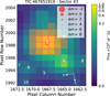 |
Fig. 1 Target pixel file from the TESS observations in Sector 43, centred on TOI-4602, which is highlighted with a white cross. The orange squares indicate the SPOC pipeline aperture, while sources from Gaia DR3 catalogue (Gaia Collaboration 2023) are overplotted with circles whose sizes are proportional to the Gaia magnitude difference with respect to our target. Grey arrows show the direction of the proper motions for all sources in the field. The colour bar indicates the electron counts per pixel. |
4 The host star
4.1 Spectroscopic stellar properties
To derive the effective temperature (Teff), the surface gravity (log g), the micro-turbulence velocity parameter (ξ) and the iron abundance ([Fe/H]) of the host star, we analysed the co-added spectrum built from individual HARPS-N spectra extracted with the standard DRS pipeline. The final signal-to-noise ratio of the co-added spectrum was ∼770 at ∼6000 Å. Given the relatively old age of the target, we applied the standard spectroscopic analysis method based on equivalent widths (EW) of iron lines to derive the stellar parameters. Specifically, Teff and log g were inferred by imposing excitation and ionization equilibria in LTE, while ξ was determined by minimizing the trend between Fe I abundances and the reduced equivalent widths log(EW/λ).
The EWs of carefully selected iron (Fe) lines (see Baratella et al. 2020 for the complete line list) were measured using the automatic tool ARES (v2.0, Sousa et al. 2015). Lines with uncertainties larger than 10% were rejected from the analysis, together with strong lines with EW> 120 mÅ. We finally used the pymoogi code (Adamow 2017), which is a Python wrapper of the MOOG code (Sneden 1973), to derive the stellar parameters and the Kurucz model atmospheres linearly interpolated from the grid by Castelli & Kurucz (2003). The final values are reported in Table 1. Our inferred spectroscopic Teff agrees perfectly with the estimate obtained using various photometric colour indexes and the colte tool developed by Casagrande et al. 2021. The photometric temperatures indeed vary between 5825±117 K in (RP − J) and 6027±77 K in (G − BP), with a weighted mean of 5946±58 K. The spectroscopic log g of 4.34±0.10 dex is consistent with the value derived from Gaia parallax and the mass value of 1.11 M⊙ reported in Paegert et al. (2021). We also derived the projected rotational velocity (v sin i) of TOI-4602 using the calibration between the FWHM of the CCF and the v sin i established by Rainer et al. (2023). The resulting value is presented in Table 1. We also detected the presence of the lithium absorption line at ∼6707.8 Å. We measured an equivalent width of EWLi = 36.5 ± 0.5 mÅ and, adopting the spectroscopic parameters measured in this work, we determined a lithium abundance of A(Li)NLTE=2.26±0.04 dex, after applying the corrections for non-local thermodynamic equilibrium effects by Lind et al. (2009). Based on empirical isochrones by Jeffries et al. (2023), and using the EWLi and Teff values with the EAGLES code, we derived an age of  Gyr. The value of the lithium abundance, combined with the effective temperature derived above, places the target coherently with members of the M67 open cluster (∼4.5 Gyr; Pasquini et al. 2008).
Stellar parameters of TOI-4602.
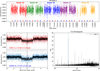 |
Fig. 2 (Top panel) Normalized TESS PDCSAP light curves from all available sectors. The out-of-transit data have been binned to 20 minutes to improve the signal-to-noise ratio, while the in-transit data are kept at the original cadence to preserve the transit shape. Red and blue triangles mark the positions of odd and even transits, respectively. BTJD refers to the Baycentric TESS Julian Date, which is the time stamp measured in BJD and offset by 2 450 000.0. Dots in different colours represent different TESS sectors, with vertical dashed lines indicating the boundaries between them. (Bottom left panels) Odd and even transits folded using a period of 3.98 days. The consistent transit depths between odd and even transits show no evidence of alternating primary and secondary eclipses, disfavouring an eclipsing binary scenario at twice the orbital period. Black curves show smoothed light curves obtained via a moving average. (Bottom right panel) TLS periodogram of TOI 4602 b light curves. The highest peak corresponds to the main transit signal at P ≈3.98 days. The additional secondary peaks visible in the periodogram correspond to harmonics (e.g. P/2, 2P) and aliases of this primary periodicity. |
4.2 Mass, radius, and age
The Galactic spatial-velocity components (U, V, W) of TOI-4602 are computed from the stellar RV together with Gaia parallaxes and proper motions (Gaia Collaboration 2023) following the procedure described in Maldonado et al. (2010). To correct these velocities to the Local Standard of Rest (LSR), we adopted the recent solar motion parameters (U⊙, V⊙, W⊙) = (12.9, 12.0, 7.8) km s−1 from Bienaymé et al. (2024). The derived values are provided in Table 1. To classify the star as belonging to the thin/thick disc population, we adopted the methodology developed by Bensby et al. (2003, 2005), based on the relative kinematic probabilities Pthick/Pthin and Pthick/Phalo. We derived the following values: Pthin = 2.13 × 10⁻⁸, Pthick = 1.56 × 10⁻⁸, and Phalo = 4.99 × 10⁻¹¹. These result in a relative probability ratio of Pthick/Pthin = 0.73, with Pthick/Phalo ≫ 1. According to the adopted framework, thin disc stars are defined by Pthick/Pthin < 0.1, while thick disc stars require Pthick/Pthin > 10. Since our value falls within the intermediate range (0.1 < Pthick/Pthin < 10), TOI-4602 is formally classified as a transition star showing intermediate kinematics. Following the method of Almeida-Fernandes & Rocha-Pinto (2018), we also estimated a kinematic age of 11 ± 3 Gyr, which, despite the inherent uncertainties of this method for single objects, points towards an old stellar population.
Moreover, we also computed stellar ages (and masses) from isochrone fittings (and evolutionary tracks). We therefore considered the PARSEC model by Bressan et al. (2012) and the PARAM interface2 (version 1.5, da Silva et al. 2006). This code considers as input some observational parameters (effective temperature, parallax, apparent V magnitude, and iron abundance) to perform a Bayesian determination of the most likely stellar intrinsic properties, appropriately weighting all the isochrone sections that are compatible with the observational parameters. A flat distribution of ages with a range of 0.1–15 Gyr was considered as priors for the analysis. We considered as effective temperature, stellar gravity and iron abundance those values we derived as described in Section 4.1. We obtained in this way a system age of  Gyr , a stellar mass of 0.90±0.02 M⊙ and a stellar radius of
  , where the uncertainties are those provided by the PARAM tool and do not include possible systematic uncertainties in the adopted stellar models.
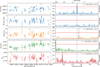 |
Fig. 3 Spectroscopic time series and GLS periodogram. Left: HARPS-N spectroscopic time series analysed in this work. From top to bottom, the panels show the RVs, RV residuals, BIS, log |


4.3 Stellar activity
We characterized the activity level of the host star by analysing the chromospheric log R’HK index. The time series (see Fig. 3 and Table A.1) shows a stable mean log  using standard (B–V) calibration. Adopting the Teff-based calibration by Lorenzo-Oliveira et al. (2018), we find log
  . Using the recent relation by Carvalho-Silva et al. (2025) for [Fe/H] = –0.3, this yields an age of 8.0–9.5 Gyr. This range is consistent with both the isochronal and kinematic ages, indicating TOI-4602 is an old star likely in the 8.0–9.0 Gyr range.
Given the low activity level, the search for a rotational signal proved to be challenging. We analysed both TESS photometry and spectroscopic activity indicators to determine the stellar rotation period (Prot), but we did not obtain a direct measurement. A Generalized Lomb-Scargle (GLS, Zechmeister & Kürster 2009) periodogram analysis revealed no significant periodicity in either data, although a minor, statistically not significant peak is visible in the Hα periodogram. The only noteworthy signal is a long-period peak in the log R’HK periodogram, which we interpret as a likely magnetic activity cycle rather than rotation. Using the mean log  value and the star’s B-V colour (Table 1), the relation from Noyes et al. (1984) yields an empirical period of Prot ∼ 17 days.
Finally, in the absence of direct X-ray observations of TOI-4602, we adopted the prediction of a X-ray luminosity between Lx = 6 × 1026 and 2 × 1027 erg s−1 based on the stellar age (Mamajek & Hillenbrand 2008). Hence, we assume  for deriving the high-energy irradiation of the planetary atmosphere, in line with the expectation for a Sun-like star.
5 Analysis
5.1 Detection and vetting of TOI-4602 b
An alert for a planet candidate around TOI-4602 was released by the TESS Mission on 2021 November 2, when the SPOC pipeline (Jenkins et al. 2016) at NASA Ames Research Center identified a candidate exoplanet with a period of 3.98 days. The planetary nature of this target has already been statistically validated using TRICERATOPS (Giacalone & Dressing 2020) by Hord et al. (2024). In this section, we provide additional evidence supporting the planetary nature of TOI-4602 b. We first detrended (flattened) the light curves of TOI-4602 using the Savitzky–Golay filter implemented in lightkurve, masking the likely transit events based on the ephemeris provided by the SPOC pipeline to build the model. We then computed the Transit Least Squares (TLS) periodogram of the detrended light curve, which combines all available TESS sectors, to search for transit signals with periods between 1 and 100 days using the Python package transitleastsquares (Hippke & Heller 2019) . The periodogram reveals a significant peak at P ∼ 3.98 days, with a Signal Detection Efficienty (SDE) of ∼45, and a stacked S/N ∼9. In Fig. 2, the positions of the odd and even transits are indicated with red and blue triangles, respectively. To verify the consistency of the transit depths, we compared the phase-folded light curves of odd and even transits. The resulting difference in depth corresponds to a significance of approximately 0.1σ, indicating that the depths of odd and even transits are consistent within the uncertainties and supporting the planetary nature of TOI-4602 b.
5.2 Photometry time-series analysis
To assess the transit signal robustness, we computed TLS periodograms for individual TESS sectors, confirming the ∼3.98-day signal. An inspection of the residuals revealed no other significant peaks, suggesting no evidence of additional transiting planets within the period range probed by TESS.
We performed a global photometric modelling of all TESS sectors within a Bayesian framework using PyORBIT (Malavolta et al. 2016, 2018), which is adopted consistently throughout this work for all orbital analysis. We simultaneously modelled each transit using the batman package (Kreidberg 2015), fitting the following parameters: orbital planetary period (P), central time of transit (T0), planetary-to-star ratio (Rp/R⋆), impact parameter b, stellar density (ρ⋆, in solar units), quadratic limb-darkening (LD) coefficients u1 and u2 adopting the LD parametrization (q1 and q2) introduced by Kipping (2013a), and photometric jitter terms to account for unmodelled effects (e.g. short-term stellar activity) or any underestimated uncertainties. Before proceeding with the PyORBIT analysis, we estimated the limb-darking coefficients and their uncertainties assuming a quadratic law using the PyLDTk package (Parviainen & Aigrain 2015), which is based on the spectrum library by Husser et al. (2013), by computing them specifically for the TESS passband. Using the effective temperature, log g, and metallicity reported in Table 1, we initially derived u1 = 0.3876 q± 0.0003 and u2 = 0.1413 ± 0.0008. Following Patel & Espinoza (2022), we adopted broader Gaussian priors with uncertainties of 0.2 for both coefficients to mitigate potential systematic discrepancies between theoretical models and TESS observations during the PyORBIT global fit. In addition, we adopted Gaussian priors of the following parameters (see Table B.1 for details): the orbital period, as indicated by the TLS periodogram; the transit time given by the first predicted transit, and the stellar density (0.71 ± 0.16 ρ⊙) estimated from the stellar mass and radius in Table 1. Following standard procedure with PyORBIT, we first performed a global optimization of the model parameters by executing a differential evolution algorithm implemented via PyDE3 (Storn & Price 1997). This was followed by a Bayesian analysis of each selected light curve around each transit using the affine-invariant ensemble sampler (Goodman & Weare 2010) for Markov chain Monte Carlo (MCMC) implemented within the package emcee (Foreman-Mackey et al. 2013). We employed 8ndim walkers (where ndim is the number of free parameters) for 50 000 generations with PyDE, followed by 150 000 steps with emcee, applying a thinning factor of 100 to reduce the effects of the chain auto-correlation. The first 25 000 steps were discarded as burn-in phase, after verifying convergence through the Gelman-Rubin statistic (Gelman & Rubin 1992). According to this analysis, the planetary radius is Rp = 2.45±0.23 R⊕ with TOI-4602 b orbiting around its star with a planetary period of  days, which is compatible with the results obtained from the TLS analysis and those given by the SPOC pipeline.
To search for perturbations potentially induced by additional non-transiting planets, or by bodies not detected by TESS, we investigated the presence of transit timing variations (TTVs) using the approach described in Naponiello (2026). We don’t find compelling evidence for significant timing modulations with a semi-amplitude upper limit of 3.5 minutes. In particular, the difference in BIC between the linear and sinusoidal models is slightly below the commonly adopted significance threshold of 10 (Fig. C.1), and the scatter statistic,  (Naponiello 2026), is close to unity, supporting this non-detection.
5.3 Spectroscopic time-series analysis
Figure 3 shows the time series and the GLS periodograms of HARPS-N RVs and all activity indicators. Regarding the planetary signals, we identified a strong peak in the RV periodogram (FAP < 0.1%) at the same period as the photometric signal. This feature is absent in all stellar activity indicators, supporting a planetary origin for the signal. To verify the presence of additional companions, we subtracted the sinusoidal model corresponding to this main peak from the RV time series (pre-whitening). The resulting residuals and their corresponding GLS periodogram, shown in the second panels from the top in Figure 3, do not exhibit any further significant peaks, indicating that no other signals are detectable above the noise level. In terms of stellar activity, a long-term trend is visible in the log  time series, highlighted by the sinusoidal fit overplotted in the panel. The corresponding periodogram shows a significant peak around 197 days, which could suggest a stellar magnetic cycle. However, as our baseline covers less than one complete cycle, this period remains approximate. Aside from this long-term modulation, no other significant peaks were detected in the activity periodograms, consistent with the average value of the
  , which indicates a low level of stellar activity for the host star.
Following the detection of a significant RV signal, we proceeded with the full orbital analysis of the RV dataset of TOI-4602 using PyORBIT, with the aim of determining the planetary mass. We adopted the same PyORBIT configuration as described in Section 5.2. In addition to the previous parameters, we included the systemic RV (offset), and the RV semi-amplitude (K) as free parameters. We tested the following models:
A single planet on a circular orbit, without stellar activity correction (Model 1, M1).
Two planets on circular orbits, to investigate the possibility of an additional companion (Model 2, M2).
A single planet on a circular orbit with quasi-periodic Gaussian Process (GP) to account for potential stellar activity signals (Model 3, M3).
A single planet on an eccentric orbit (Model 4, M4).
We obtained the following Bayesian Information Criterion (BIC) values: BIC(M1) = 188.8, BIC(M2) = 199.5, BIC(M3) = 204.9, BIC(M4) = 196.0. To select the best model, we follow the criteria from Kass & Raftery (1995), where evidence favouring the model with the lower BIC is considered ‘strong’ for |∆BIC| > 6 and ‘very strong’ for |∆BIC|> 10. Based on this, we find that M1 is very strongly preferred over M2 and M3 (∆BIC21 = 10.7, ∆BIC31 = 16.1), and strongly preferred over M4 (∆BIC41 = 7.2).
In addition to these scenarios, we explicitly tested the inclusion of a linear velocity trend to account for potential long-term drifts. This model yielded a BIC = 192.47, resulting in a ∆BIC = 3.67 in favour of the simpler 1-planet circular model (M1). We also explored a broader two-planet scenario by searching for additional Keplerian signals with periods up to 300 days, which was decisively disfavoured with a BIC = 207.23 (∆BIC ≈ 18.4 relative to M1). Considering the results of all these tests, we find that M1 is statistically preferred over all other configurations. Consequently, we adopt Model 1 as the best representation of the RV data, from which we derived a RV semi-amplitude of  m/s, a planetary mass of
  for TOI-4602 b, and an orbital period of
  days, in excellent agreement with the photometric period. We further quantify the detection sensitivity of our RV time-series in Appendix D, along with the Proper Motion anomaly (PMa) revealed for this star by the Hipparcos-Gaia Catalogue of Accelerations (HCGA; Brandt 2018).
5.4 Joint radial velocity and photometry analysis
A joint transit and RV analysis was performed using PyORBIT. For this global modelling, we switched from the MCMC sampler used in the previous sections to the Multinest Nested Sampling algorithm via PyMultiNest (Feroz et al. 2009; Buchner et al. 2014). This choice was motivated by the need to directly compute the Bayesian Evidence (𝒵) of the models, which provides a more rigorous statistical metric for model comparison than the BIC approximation, particularly when combining heterogeneous datasets (RV and photometry) and exploring high-dimensional parameter spaces.
Based on our previous findings, we adopted a one-planet model for the combined modelling. This approach enabled us to derive consistent and precise estimates of the orbital and physical parameters of TOI-4602 b by combining the complementary constraints from both transit and RV data. In particular, the joint fit yields a self-consistent determination of the planetary density, based on independently derived – yet coherently modelled – measurements of the planet’s radius and mass. Although the RV-only analysis strongly favours a circular orbit (M1), we decided to test the eccentric model also. This allows us to verify if the inclusion of the transit data introduces any preference for a non-circular orbit, and to derive more robust uncertainties for the planetary parameters by marginalizing over the eccentricity. The planetary system parameters derived from the joint fit for both the circular and eccentric models are listed in Table B.1.
We compared the models using the Bayes factor Bij = 𝒵i/𝒵j. Following the scale of Jeffreys (1998), a difference in log-evidence ∆ ln 𝒵 > 2.5 corresponds to moderate evidence, while ∆ ln 𝒵 > 5 indicates strong evidence in favour of the model with higher probability. The eccentric model (using a uniform prior on e) yields a log-evidence of ln 𝒵e = 468337.8 ± 0.3, compared to ln 𝒵c = 468334.3 ± 0.3 for the circular case. This results in a Bayes factor of ∆ ln 𝒵 = 3.5 in favour of the eccentric solution (e = 0.23 ± 0.06), corresponding to moderate evidence according to the scale of Jeffreys (1998). To ensure this preference was not an artefact of the prior, we performed additional fits using physically motivated distributions: a Beta distribution (α = 0.867, β = 3.03; Kipping 2013b) and a Half-Gaussian prior (σ = 0.32), the latter being specifically recommended for small planets (Van Eylen et al. 2019). These tests confirm the prior-independence of the result: the Beta prior yields  and ∆ ln 𝒵 ≈ 3.7, while the Half-Gaussian prior results in
  and ∆ ln 𝒵 ≈ 4.3. Although the eccentric model is statistically favoured across all scenarios, the evidence remains below the ‘decisive’ threshold (∆ ln 𝒵 < 5). Furthermore, the planetary parameters remain consistent within 1σ regardless of the model choice; for instance, the eccentric fit yields a mass of 6.2 ± 0.9 M⊕, fully compatible with the circular case. Given the moderate significance of the improvement, the strong preference for circularity in the RV-only analysis, and the robustness of the planetary parameters against the model choice, we adopt the circular solution as our fiducial model. This provides a conservative description of the system with fewer free parameters, despite we cannot rule out a moderate eccentricity.
Fig. 4 shows the RV and transit data with the best-fit circular models overplotted. Based on this adopted solution, we determine that the transiting object is a sub-Neptune planet with a mass of Mp = 5.5 ± 0.9 M⊕ and a radius of 2.5 ± 0.2 R⊕, yielding a density of ρp = 2.2 ± 0.8 g cm−3. The planetary mass derived from the joint analysis is consistent with that obtained from our RV-only analysis. As expected, the combined fit allows a more precise determination of the orbital period of TOI-4602 b ( days), in excellent agreement with the photometric period.
5.5 Insolation, equilibrium temperature, scale height, and transmission spectroscopy metric
In addition to all the derived planet parameters, reported in Table B.1, including the inclination, impact parameter, and semi-major axis, we calculated an insolation of 664 ± 42 S⊕. We estimated the planet’s equilibrium temperature (Teq) assuming a Bond albedo of A = 0.3 (the same as Earth’s) and full heat redistribution between the day and night sides. This yields an equilibrium temperature of Teq = 1344 ± 80 K. Assuming a cloud-free, H2-dominated atmosphere, we estimated the atmospheric scale height to be H = 538 ± 140 km. This corresponds to a transmission spectral feature amplitude of 60±20 ppm, estimated using the relation  (Kreidberg 2018). We note that the assumption of a hydrogen-dominated atmosphere represents the most optimistic case for transmission spectroscopy. For super-Earths, heavier atmospheric compositions (e.g. dominated by water vapour or CO2) are also plausible and would imply higher mean molecular weights. In such scenarios, the scale height-and consequently the amplitude of spectral features-would be significantly reduced, making atmospheric characterization more challenging. We also computed the transmission spectroscopy metric (TSM) following the definition by Kempton et al. (2018). We obtained a value of TSM = 140 ± 54, which lies above the threshold of 90 suggested by Kempton et al. (2018), indicating that the planet is a promising target for atmospheric characterization.
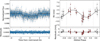 |
Fig. 4 Modelling of photometric and spectroscopic time series obtained from the joint fit assuming a circular model. (Left) Photometric modelling of the TOI-4602 b planetary signal. The top panel displays the normalized, phase-folded TESS transits overlaid with the best-fit model (black line), while the bottom panel shows the residuals between the observed data and the model. (Right) Phase-folded RV fit of TOI-4602 b planetary signal. The reported error bars include the jitter term, added in quadrature. The bottom panel displays the residuals of the fit. |
6 Mass-radius diagram and internal structure
In this section we first use our measurements of the planet parameters to investigate the bulk structure of TOI-4602 b in the context of the photo-evaporation as the main driver of the evolution of these close-in, low-mass planets.
Figure E.1 shows the position of TOI-4602 b in a mass-radius diagram, along with a sample of well-characterized exoplanets with a mass uncertainty better than 20% and a radius uncertainty better than 10%. The parameters for the known exoplanets were taken from NASA Exoplanet Archive (Christiansen et al. 2025). We included theoretical mass-radius relationships for different bulk compositions: bare rocky planets with 100% Fe, 33% Fe + 66% MgSiO3, 20% Fe + 80% MgSiO3, 100% MgSiO3 and Earth-like rocky core with H/He envelopes of 0.3% and 1% by mass. These models assume a surface pressure of 1 mbar and an equilibrium temperature of 1000 K. Although models with high amounts of surface water of tens of weight percent could in principle fit TOI-4602 b, we refrain from plotting such models as they are not plausible given interior-atmosphere interactions (Luo et al. 2024; Werlen et al. 2025). Specifically, global equilibrium calculations predict a universal upper limit on the available surface water of few percent (Werlen et al. 2025), even if large amounts of water are accreted during formation. The majority of accreted water is chemically destroyed and stored in the metal phase of sub-Neptunes (Schlichting & Young 2022). Sub-Neptunes are thus hosting enriched H/He envelopes, chemically coupled to their deeper magma oceans.
In order to determine the possible interior compositions and structures, we employ an inference framework (De Wringer et al. 2026) using the physical forward model of Dorn et al. (2015, 2017) with recent updates from Dorn & Lichtenberg (2021); Luo et al. (2024). The inference framework is a surrogate-accelerated Bayesian inference, in which the computationally expensive physical forward model is replaced with a fast polynomial chaos-Kriging (PCK) surrogate directly within an MCMC sampling loop (Marelli & Sudret 2014). For this inference, both the circular and eccentric models were tested. The surrogate model provides high quality fits with R-squared values (coefficient of determination). For the circular model, the fits are 0.9999 and 0.9849 for the planetary mass and radius, respectively, and for the eccentric model, the fits are 0.9999 and 0.9862 for the planetary mass and radius, respectively. Also, the surrogate root mean square errors are well below observational uncertainties with the same values for both models: 0.0006 and 0.06 for planetary mass and radius, respectively. Those errors of the model uncertainty are accounted for in the likelihood function.
The interior model assumes an Earth-like rocky interior with an iron-dominated core, a silicate mantle and an enriched H/He envelope on top. The core-mantle mass ratio is set to 0.325:0.675. We allow for both liquid and solid phases in mantle and core layers. For liquid core iron and iron alloys we use the equation of state (EOS) by Luo et al. (2024). For solid iron, we use the EOS for hexagonal close packed iron (Hakim et al. 2018; Miozzi et al. 2020). For pressures below ≈125 GPa, the solid mantle mineralogy is modelled using the thermodynamical model PERPLE_X (Connolly 2009) considering the system of MgO, SiO2, and FeO. At higher pressures we define the stable minerals a priori and use their respective EOS from various sources (Hemley et al. 1992; Fischer et al. 2011; Faik et al. 2018; Musella et al. 2019). The liquid mantle is modelled as a mixture of Mg2SiO4, SiO2 and FeO (Melosh 2007; Faik et al. 2018; Ichikawa & Tsuchiya 2020; Stewart et al. 2020), and mixed using the additive volume law. We assume an adiabatic temperature profile for the core and mantle with possible temperature jumps at the core-mantle-boundary depending on melt temperatures.
The H2–He–H2O atmosphere layer is modelled using the analytic description of Guillot (2010) and consists of an irradiated layer on top of a non-irradiated layer in radiative-convective equilibrium. The water mass fraction is given by the metallicity Z and the hydrogen-helium ratio is set to solar. The two components of the atmosphere, H2/He and H2O, are again mixed following the additive volume law and using the EOS by Saumon et al. (1995) for H2/He and the ANOES EOS (Thompson 1990) for H2O. The transit radius of a planet is defined where the chord optical depth reaches 0.56 (Des Etangs et al. 2008). For each model realization, the planet intrinsic luminosity is calculated following (Mordasini 2020) and is a function of planet mass, atmospheric mass fraction and age.
While fixing an Earth-like core-mantle ratio, we find that the planet is best described by an envelope mass of 0.05 M⊕ ± 0.03 for both models. The metallicity is found to be  for the circular model, and
  for the eccentric one. These results are visible in Fig. E.2 and Table E.1. Although we obtain two different planetary masses, they are compatible at 1-sigma and lead to the same scientific results. This scenario is compatible with the expected atmospheric loss as described in the next section.
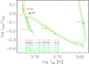 |
Fig. 5 Evolutionary track of TOI-4602 in the effective temperature-bolometric luminosity plane. The red circle marks the current location of the star on the track. |
7 Photoevaporation and long-term evolution
We investigated TOI-4602 b’s long-term atmospheric evolution, considering the significant UV-driven mass loss typical of close-in sub-Neptunes, and estimated how much atmosphere the planet may have retained over millions of years.
We selected a MESA evolutionary track (Choi et al. 2016), compatible with the star’s position at its nominal age in the theoretical Lbol vs. Teff diagram. We considered a grid of evolutionary tracks for stars with masses and metallicities equal to the nominal values for TOI-4602, or equal to ±1σ values in both parameters (9 tracks in total). Some of them are shown in Fig. 5. We found that the best match is achieved with the track of a star with the nominal mass of TOI-4602 and metallicity [Fe/H] = −0.29 (−1σ). We used this track for modelling the bolometric irradiation of the planet and therefore its equilibrium temperature, as well as the core-envelope structure during evolution, taking into account the gravitational shrinking (Fortney et al. 2007). To model the evolution of high-energy irradiation, we assumed as anchor point for the X-ray luminosity at the current age the value Lx = 1 × 1027 erg/s, determined in Sect. 4.3.
In Fig. 6, we show the time evolution of the X-ray (5–100 Å), EUV (100–920 Å), and XUV (X+EUV) luminosities, according to two different models: the Penz et al. (2008) X-ray luminosity evolution coupled with the Sanz-Forcada et al. (2025) X-ray to the EUV scaling law (PSF model) or, alternatively, adopting the Johnstone et al. (2021) prescription (Jo model). In the former case, the current X-ray luminosity appears to be near the median for solar-mass stars at the nominal age of TOI-4602. In the second case, we selected the evolutionary track corresponding to the lowest 2% percentile of the activity distribution appropriate for stars with a mass of 0.9 M⊙. Nonetheless, the Johnstone et al. (2021) evolutionary path yields an X-ray luminosity that is about a factor 6 higher than the nominal value determined above, and significantly outside the uncertainty range. Hence, with the Jo-model assumption, the high-energy irradiation of the planet for ages >800 Myr is likely overestimated.
Considering the constraints on the activity level provided by the age and the chromospheric Ca II H&K index (Sect. 4.3), we also explored the results of photo-evaporation assuming the Penz et al. (2008) evolutionary tracks anchored at the extreme values of the uncertainty range: Lx = 2 × 1027 erg/s at an age of 5 Gyr, or Lx = 6 × 1026 erg/s at an age of 8.6 Gyr.
In summary, we investigated the planetary photoevaporation with four evolutionary tracks for the high-energy (X-ray + EUV) radiation: two tracks in which we fixed the stellar age at 6.8 Gyr, and we assumed either the PSF model or the Jo model (PSF-6.8 or Jo-6.8, respectively), and two more tracks at ages of 5 Gyr or 8.6 Gyr, both following the PSF model (PSF-5 and PSF-8). In Fig. F.1, we show the evolution of the mass, radius, and mass loss rate for these four different scenarios.
For the analysis of the past and future evaporative evolution, we employed the numerical code first presented in Locci et al. (2019), subsequently adapted for the study of single systems (Maggio et al. 2022) and more recently described in Mantovan et al. (2024). Assuming an Earth-like core composition, we first calculated the planet’s internal structure, finding a core mass of approximately 5.5 M⊕ and a radius of around 1.56 R⊕, which implies an atmospheric fraction of approximately 1.5%. These values are quite insensitive to variations in age. This finding is in good agreement with the results of Section 6. We then computed the past and future evolution of key planetary parameters, such as the atmospheric fraction and total radius, while keeping the mass and core radius constant over time. In order to calculate the mass-loss rates we use the ATES analytical approximation, which includes different regimes such as energy limited and recombination limited (Caldiroli et al. 2021). Assuming solar abundances for the atmosphere, we followed the atmospheric evolution back to an age of 10 million years, which we assumed to be the time when the accretion disc was fully dissipated and the planet had reached its final orbit, and forward in time up to an age of 10 Gyr. The calculated initial mass and radius of the system depend on the XUV evolutionary track used. Overall, for the initial mass we predict values in the range 31.1–33.8 M⊕, with corresponding radii 14.8–14.7 R⊕.
Furthermore, we found that for the PSF-6.8. Jo-6.8 and PSF-5 tracks, the planet is currently undergoing the transition across the radius valley. In these scenarios, it will lose its entire remaining atmosphere within approximately 2.6, 0.8, and 1.4 Gyr from now, respectively (i.e. reaching a bare-core state at an age of about 9.4, 7.6, and 6.4 Gyr). Therefore, under these assumptions, the planet will eventually cross the radius valley entirely, ending its evolution on the small-radius peak of the bimodal distribution with a mass and radius equal to that of its core. In contrast, for the PSF-8 track (which assumes a current age of 8.6 Gyr and a milder XUV history), the planet is currently at the end of its active evaporative phase. It is able to retain a small atmospheric fraction against further photoevaporation, meaning its radius will stall near its current value of about 2 R⊕. In this scenario, the planet’s evolution halts just above the radius valley, remaining part of the sub-Neptune population.
We also explored a case where we assumed a metallicity 50 times that of the Sun for the calculation of the envelope radius (Lopez & Fortney 2014), finding similar behaviour to the previous case for all four tracks, in particular in the future evolution. The differences between the two scenarios are more significant in the initial phases, where the planet exhibits a larger radius, in the case of high metallicity. Consequently, it is subject to greater evaporation, which in turn requires a higher initial mass that ranges from 38 to 42 M⊕, depending on the evolutionary track considered. The time evolution of planetary parameters for the enhanced abundance case is shown in Fig. F.2.
Finally, we simulated the case with eccentric orbit, resulting in a higher planetary density compared to the circular-orbit scenario. As a consequence, TOI-4602 b has a slightly greater resistance to photoevaporation. Although the effect is modest, it implies that in the three cases in which the planet completely lost its atmosphere in the circular-orbit scenario, the atmosphere is still lost but at slightly later ages. In particular, this occurs at about 10 Gyr for the PSF-6.8 case, 7.8 Gyr for the Jo-6.8 case, and 6.7 Gyr for the PSF-5 case. Otherwise, the evolutionary curves remain similar to those of the circular-orbit case.
In conclusion, we find that the planet’s final radius is largely independent of the assumed initial atmospheric metallicity, although higher metallicities strongly impact the early evolutionary phases. Crucially, the current evolutionary stage and the ultimate fate of TOI-4602 b are highly sensitive to the stellar age and the assumed XUV history. In three out of four analysed XUV scenarios, the planet is currently still undergoing atmospheric escape and will eventually cross the radius valley, ending as a bare core on the small-radius peak. The only exception is the oldest scenario (8.6 Gyr) coupled with the PSF-8 XUV track; here, the planet has already ceased significant evaporation and its evolution will safely terminate above the radius valley (∼2 R⊕), retaining a thin envelope.
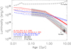 |
Fig. 6 Time evolution of X-ray (5–100 Å), EUV (100–920 Å), and total XUV luminosity of TOI-4602, according to Penz et al. (2008) and the X-ray/EUV scaling by Sanz-Forcada et al. (2025) (red lines) and according to Johnstone et al. (2021) (blue lines). Uncertainties on the age and X-ray luminosity of TOI-4602 q(square symbol) are also indicated, with respect to the nominal value of Lx = 1027 erg/s at 6.8 Gyr. The grey area is the original locus for dG stars in Penz et al. (2008). For comparison purpose, we also show the current position of the Sun and the full range of variability during an 11-year magnetic cycle. |
8 Atmospheric simulations
TOI-4602 b is an excellent candidate for atmospheric characterization due to its high TSM (Section 5.5) and the brightness and quietness of its host star. Here, we investigate the capability of Ariel and JWST (Gardner et al. 2006) to characterize its atmosphere via retrievals on simulated 1× solar-metallicity transmission spectra. We assumed a cloud-free, isothermal, plane-parallel atmosphere with constant molecular abundances, including Rayleigh scattering and Collision Induced Absorption (CIA) of H2–H2/H2–He (Richard et al. 2012; Cox 2015). Forward and retrieval models utilize ExoMol (Tennyson et al. 2016) and HITEMP (Rothman & Gordon 2008) opacities for H2O (Polyansky et al. 2018), CO (Li et al. 2015), CO2 (Yurchenko et al. 2020), CH4 (Yurchenko et al. 2024), SO2 (Underwood et al. 2016), and K (Allard et al. 2016). Although CH4 likely dissociates into CO above ∼1000 K, we included it to probe potential disequilibrium chemistry and constrain upper limits.
Ariel simulations were performed using the TauREx framework (Al-Refaie et al. 2021, 2022). Forward spectra, based on parameters in Tables 1 and B.1, were convolved with the Ariel-Rad instrument model (v. 2.4.26, Mugnai et al. 2020; Payload v. 0.0.17, ExoRad v. 2.1.111, Mugnai et al. 2023) to generate input spectra. We focused on Tier 2 resolution (Tinetti et al. 2022), binning the data to R = 10, 50, and 20 in FGS-NIRSpec (1.1–1.95 µm), AIRS-Ch0 (1.95–3.9 µm), and AIRS-Ch1 (3.9–7.8 µm), respectively4. Using ArielRad, we determined that 20 transits are required to achieve the Tier-2 S/N, assuming Gaussian noise scaled by the square root of observations. Retrievals employed the PYMULTINEST sampler with 500 live points, a 0.5 evidence tolerance, and non-informative uniform priors on abundances.
We simulated and retrieved JWST observations using the PYRAT BAY framework (Cubillos & Blecic 2021), adopting the same atmospheric assumptions as the Ariel case. Using the GEN TSO simulator (Cubillos 2024), we generated transit depths and uncertainties for a single transit combining NIRISS/SOSS (SUB204STRIPE), NIRSpec/BOTS (G395H), and MIRI/LRS to cover 0.65–12 µm. Retrievals employed the PYMULTINEST sampler. The free parameters included isothermal temperature, reference pressure at Rp, grey cloud deck pressure, and VMRs for K, H2O, CO2, CO, CH4, and SO2.
Fig. G.1 shows the simulated transmission spectra and resulting posterior distributions for the Ariel (blue) and JWST (orange) retrieval runs. While both recover the main atmospheric constituents, differences in spectral coverage and resolution drive key discrepancies in precision. Ariel achieves higher precision on H2O (∼0.2 dex vs ∼0.5 dex) and SO2 due to its broad, continuous wavelength coverage (0.5–7.8 µm), which captures multiple water bands and the strong SO2 feature at 7.3 µm, effectively breaking parameter degeneracies. Conversely, JWST provides superior constraints on Potassium (K). In the Ariel simulations, the K-doublet signal (∼0.77 µm) falls in the blue end of the spectrum, where it is constrained by only a few photometric channels. Due to this limited spectral information, the narrow K absorption feature is highly degenerate with the spectral slope introduced by Rayleigh scattering, cloud opacity, and stellar activity. Since these strong contaminating effects are likely to be present in real observational data, the constraint on K is significantly compromised. Consequently, the resulting broad posterior is considered difficult to confidently interpret as a true atmospheric detection, highlighting the value of complementary observations between Ariel and JWST. Regarding carbon species, CO accuracy is comparable, and CH4 is correctly retrieved as an upper limit in both cases. For CO2 we noticed that the true value is slightly outside the 1σ region for both retrievals. This likely results from the relatively low CO2 abundance at 1× solar metallicity, and the blending of multiple opacities (CO, CO2, H2O, SO2) at around 4.0 µm, the region with the strongest CO2 absorption band. Despite the challenges linked to degeneracies in the Potassium band, the Ariel high-precision constraints on broadly distributed key species like H2O and SO2 demonstrates the robustness and effectiveness of its wide-field survey approach for characterizing a large sample of exoplanet atmospheres.
9 Discussion and conclusions
We have presented a comprehensive analysis of the TOI-4602 system, combining TESS photometry with high-precision RVs from HARPS-N obtained within the ArMS project. Our joint analysis tested both circular and eccentric orbital models, confirming the presence of a transiting planet with a period of 3.98 days. While both models yield consistent planetary mass and radius estimates, the Bayesian evidence shows a moderate preference for the eccentric solution. However, interpreting this eccentricity requires a consistent physical model that accounts for the system’s advanced age (8–9 Gyr) and the planet’s internal composition. The circularization timescale of the orbit of TOI-4602 b is highly uncertain because we do not know its modified tidal quality factor Q′ that quantifies the efficiency of tidal dissipation in its interior. If we adopt a value of Q′ = 105 that is similar to that of Uranus (see Ogilvie 2014), and if we use the tidal model of Leconte et al. (2010) when computing the product of the tidal time lag ∆t by the Love number k2 with the simple formula k2∆t = 3/(2Q′n), where n = 2π/Porb is the orbital mean motion, we obtain a tidal decay timescale τe ≡ |e/ė| ∼ 3.4 Gyr. This timescale is shorter, but still comparable with the age of the system. Therefore, in this scenario, a remarkable primordial eccentricity could not have been completely damped during the main-sequence lifetime of the system. On the other hand, if we assume that the planet has an inner rocky core that dominates tidal dissipation, surrounded by a thick hydrogen envelope that is not appreciably contributing to tidal dissipation, the situation changes. Considering a rocky core of radius 1.56 R⊕ (cf. Sect. 7) and Q′ = 103, we obtain a tidal damping timescale of 0.2 Gyr, which is much shorter than the age of the star. In this scenario, any primordial eccentricity has certainly been damped at the present evolutionary stage of the system. These estimates are valid assuming no additional body in the system is able to gravitationally excite the eccentricity of TOI-4602 b. Our internal structure modelling revealed that TOI-4602 b is indeed best described by a rocky core surrounded by a tenuous envelope (∼1% by mass). This composition strongly points towards the low-Q′ scenario (τe ∼ 0.2 Gyr), rendering the survival of primordial eccentricity physically implausible.
To rigorously assess the presence of perturbers, we performed an injection-recovery test combining HARPS-N RVs and proper motion anomalies, finding sensitivity to Jupiter-mass planets up to ∼1 AU. These observational constraints effectively rule out secular perturbations as the cause of the eccentricity, since generating e ≈ 0.23 would require a massive companion at ∼0.11 AU or a compact chain at 0.07–0.08 AU, which would have been detected with high confidence. Alternative scenarios involving distant companions, such as high-eccentricity migration from >1 AU or planet-planet scattering, remain unconstrained by our data but they are physically disfavoured. The former requires a high tidal quality factor inconsistent with the planet’s likely rock-dominated structure, while the latter would require a statistically unlikely recent instability given the fast tidal damping (τe ∼ 0.2 Gyr) expected for a rocky core. Given the conflict between the rapid tidal damping expected for a rocky planet and the lack of detected close-in perturbers, we adopted the circular solution as our fiducial model, classifying TOI-4602 b as a sub-Neptune with a mass of Mp = 5.5 ± 0.9 M⊕ and a radius of Rp = 2.5 ± 0.2 R⊕, yielding a mean bulk density of ρp = 2.2 ± 0.8 g cm−3.
TOI-4602 b currently resides in the sub-Neptune regime, populating the upper peak of the bimodal radius distribution. With a radius of 2.5 ± 0.2 R⊕ and a stellar insolation of 664 ± 42 S⊕, the planet sits well above the radius valley (Fulton et al. 2017). This position is particularly interesting when considering the recent findings of Wanderley et al. (2025), who revisited the dependence of the valley on the orbital period and insolation. At such high irradiation levels and short orbital periods (P ∼ 3.98 d), many planets are expected to cross the valley due to atmospheric stripping, and thus become bare rocky cores.
Our photo-evaporation modelling (Section 7) suggests that TOI-4602 b has remained remarkably resilient in this high-insolation regime. Despite the intense hydrodynamic escape expected during the system’s youth, the planet has retained a non-negligible H/He envelope. Depending on the stellar XUV history, TOI-4602 b is either in a slow phase of atmospheric mass loss or has reached a stable configuration, offering a valuable snapshot of a sub-Neptune that has resisted complete transformation into a bare rocky core. This resilience provides a critical constraint for models of atmospheric retention and evolution for planets transitioning across the radius valley.
Finally, with a TSM of 140 ± 54, TOI-4602 b is a prime target for atmospheric characterization. Our retrieval simulations demonstrate that Ariel and JWST can effectively constrain its atmospheric composition. Spectroscopic measurements are crucial to probe the chemical inventory and thermal structure of a planet transitioning across the radius valley. Critically, resolving the abundance of species such as H2O and placing limits on the envelope metallicity would provide an independent check on our internal structure assumptions. Confirming a low-mass, high-metallicity envelope would validate the low-Q′ hypothesis, definitively closing the loop on the dynamical history of this evolved planetary system. TOI-4602 b thus stands out as a key laboratory where atmospheric characterization can directly illuminate the mechanisms sculpting the architecture of the small-planet population.
Acknowledgements
The authors acknowledge the support from ASI-INAF agreement 2021-5-HH.0, the INAF Guest Observer Grant (Normal) “ArMS: the Ariel Masses Survey Large Program at the TNG” (Prog ID: AOT48TAC_48), and the INAF Mini-Grant “Impact of planetary Masses and Radii Estimates on the Atmospheric retrievals – IMaREA”. The research activities described in this paper were carried out with contribution of the Next Generation EU funds within the National Recovery and Resilience Plan (PNRR), Mission 4 – Education and Research, Component 2 – From Research to Business (M4C2), Investment Line 3.1 – Strengthening and creation of Research Infrastructures, Project IR0000034 – “STILES – Strengthening the Italian Leadership in ELT and SKA”. C.D. acknowledges support from the Swiss National Science Foundation under grant TMSGI2_211313. This work has been carried out within the framework of the NCCR PlanetS supported by the Swiss National Science Foundation under grant 51NF40_205606. G.M. acknowledges support by the Space It Up project funded by the Italian Space Agency, ASI, and the Ministry of University and Research, MUR, under contract no. 2024-5-E.0 – CUP no. I53D24000060005. We acknowledge the Italian center for Astronomical Archives (IA2), part of the Italian National Institute for Astrophysics (INAF), for providing technical assistance, services and supporting activities of the GAPS collaboration. This work used data from the European Space Agency (ESA) mission Gaia (https://www.cosmos.esa.int/gaia), processed by the Gaia Data Processing and Analysis Consortium (DPAC, https://www.cosmos.esa.int/web/gaia/dpac/consortium). Funding for DPAC has been provided by national institutions participating in the Gaia Multilateral Agreement.
References
- Adamow, M. M. 2017, in American Astronomical Society Meeting Abstracts, 230, 216.07 [NASA ADS] [Google Scholar]
- Al-Refaie, A. F., Changeat, Q., Waldmann, I. P., & Tinetti, G. 2021, ApJ, 917, 37 [NASA ADS] [CrossRef] [Google Scholar]
- Al-Refaie, A. F., Changeat, Q., Venot, O., Waldmann, I. P., & Tinetti, G. 2022, ApJ, 932, 123 [NASA ADS] [CrossRef] [Google Scholar]
- Allard, N. F., Spiegelman, F., & Kielkopf, J. F. 2016, A&A, 589, A21 [NASA ADS] [CrossRef] [EDP Sciences] [Google Scholar]
- Aller, A., Lillo-Box, J., Jones, D., Miranda, L. F., & Barceló Forteza, S. 2020, A&A, 635, A128 [NASA ADS] [CrossRef] [EDP Sciences] [Google Scholar]
- Almeida-Fernandes, F., & Rocha-Pinto, H. J. 2018, MNRAS, 476, 184 [Google Scholar]
- Baratella, M., D’Orazi, V., Biazzo, K., et al. 2020, A&A, 640, A123 [NASA ADS] [CrossRef] [EDP Sciences] [Google Scholar]
- Batalha, N. E., Lewis, T., Fortney, J. J., et al. 2019, ApJ, 885, L25 [Google Scholar]
- Bensby, T., Feltzing, S., & Lundström, I. 2003, A&A, 410, 527 [CrossRef] [EDP Sciences] [Google Scholar]
- Bensby, T., Feltzing, S., Lundström, I., & Ilyin, I. 2005, A&A, 433, 185 [NASA ADS] [CrossRef] [EDP Sciences] [Google Scholar]
- Bienaymé, O., Robin, A. C., Salomon, J.-B., & Reylé, C. 2024, A&A, 689, A280 [NASA ADS] [CrossRef] [EDP Sciences] [Google Scholar]
- Bonomo, A. S., Naponiello, L., Sozzetti, A., et al. 2026, A&A, 707, A197 [NASA ADS] [CrossRef] [EDP Sciences] [Google Scholar]
- Borucki, W. J., Koch, D., Basri, G., et al. 2010, Science, 327, 977 [Google Scholar]
- Brandt, T. D. 2018, ApJS, 239, 31 [Google Scholar]
- Bressan, A., Marigo, P., Girardi, L., et al. 2012, MNRAS, 427, 127 [NASA ADS] [CrossRef] [Google Scholar]
- Buchner, J., Georgakakis, A., Nandra, K., et al. 2014, A&A, 564, A125 [NASA ADS] [CrossRef] [EDP Sciences] [Google Scholar]
- Burke, C. J., Christiansen, J. L., Mullally, F., et al. 2015, ApJ, 809, 8 [NASA ADS] [CrossRef] [Google Scholar]
- Burn, R., Mordasini, C., Mishra, L., et al. 2024, Nat. Astron., 8, 463 [Google Scholar]
- Caldiroli, A., Haardt, F., Gallo, E., et al. 2021, A&A, 655, A30 [NASA ADS] [CrossRef] [EDP Sciences] [Google Scholar]
- Carleo, I., Malavolta, L., Lanza, A. F., et al. 2020, A&A, 638, A5 [NASA ADS] [CrossRef] [EDP Sciences] [Google Scholar]
- Carvalho-Silva, G., Meléndez, J., Rathsam, A., et al. 2025, ApJ, 983, L31 [Google Scholar]
- Casagrande, L., Lin, J., Rains, A. D., et al. 2021, MNRAS, 507, 2684 [NASA ADS] [CrossRef] [Google Scholar]
- Castelli, F., & Kurucz, R. L. 2003, in IAU Symposium, 210, Modelling of Stellar Atmospheres, eds. N. Piskunov, W. W. Weiss, & D. F. Gray, A20 [NASA ADS] [Google Scholar]
- Castro-González, A., Demangeon, O. D. S., Lillo-Box, J., et al. 2023, A&A, 675, A52 [NASA ADS] [CrossRef] [EDP Sciences] [Google Scholar]
- Choi, J., Dotter, A., Conroy, C., et al. 2016, ApJ, 823, 102 [Google Scholar]
- Christiansen, J. L., McElroy, D. L., Harbut, M., et al. 2025, Planet. Sci. J., 6, 186 [Google Scholar]
- Cloutier, R., & Menou, K. 2020, AJ, 159, 211 [NASA ADS] [CrossRef] [Google Scholar]
- Connolly, J. A. D. 2009, The geodynamic equation of state: What and how – Connolly – 2009 – Geochemistry, Geophysics, Geosystems – Wiley Online Library [Google Scholar]
- Cosentino, R., Lovis, C., Pepe, F., et al. 2014, SPIE Conf. Ser., 9147, 91478C [Google Scholar]
- Covino, E., Esposito, M., Barbieri, M., et al. 2013, A&A, 554, A28 [NASA ADS] [CrossRef] [EDP Sciences] [Google Scholar]
- Cox, A. N. 2015, Allen’s Astrophysical Quantities (Springer) [Google Scholar]
- Cubillos, P. E. 2024, PASP, 136, 124501 [Google Scholar]
- Cubillos, P. E., & Blecic, J. 2021, MNRAS, 505, 2675 [NASA ADS] [CrossRef] [Google Scholar]
- Cutri, R. M., Wright, E. L., Conrow, T., et al. 2021, VizieR Online Data Catalog: AllWISE Data Release (Cutri+ 2013), VizieR On-line Data Catalog: II/328. Originally published in: IPAC/Caltech (2013) [Google Scholar]
- da Silva, L., Girardi, L., Pasquini, L., et al. 2006, A&A, 458, 609 [NASA ADS] [CrossRef] [EDP Sciences] [Google Scholar]
- da Silva, J. G., Figueira, P., Santos, N. C., & Faria, J. P. 2018, J. Open Source Softw., 3, 667 [Google Scholar]
- De Wringer, T., Dorn, C., Garvin, E. O., & Marelli, S. 2026, ApJ, 997, 321 [Google Scholar]
- Des Etangs, A. L., Pont, F., Vidal-Madjar, A., & Sing, D. 2008, A&A, 481, L83 [NASA ADS] [CrossRef] [Google Scholar]
- Di Maio, C., Changeat, Q., Benatti, S., & Micela, G. 2023, A&A, 669, A150 [NASA ADS] [CrossRef] [EDP Sciences] [Google Scholar]
- Dorn, C., Khan, A., Heng, K., et al. 2015, A&A, 577, A83 [NASA ADS] [CrossRef] [EDP Sciences] [Google Scholar]
- Dorn, C., & Lichtenberg, T. 2021, ApJ, 922, L4 [NASA ADS] [CrossRef] [Google Scholar]
- Dorn, C., Venturini, J., Khan, A., et al. 2017, A&A, 597, A37 [NASA ADS] [CrossRef] [EDP Sciences] [Google Scholar]
- Dos Santos, L. A. 2023, in AU Symposium, Vol. 370, Winds of Stars and Exoplanets, eds. A. A. Vidotto, L. Fossati, & J. S. Vink, 56 [Google Scholar]
- Faik, S., Tauschwitz, A., & Iosilevskiy, I. 2018, Comput. Phys. Commun., 227, 117 [NASA ADS] [CrossRef] [Google Scholar]
- Feroz, F., Hobson, M. P., & Bridges, M. 2009, MNRAS, 398, 1601 [NASA ADS] [CrossRef] [Google Scholar]
- Fischer, R. A., Campbell, A. J., Shofner, G. A., et al. 2011, Earth Planet. Sci. Lett., 304, 496 [CrossRef] [Google Scholar]
- Foreman-Mackey, D., Hogg, D. W., Lang, D., & Goodman, J. 2013, PASP, 125, 306 [Google Scholar]
- Fortney, J. J., Marley, M. S., & Barnes, J. W. 2007, ApJ, 659, 1661 [Google Scholar]
- Fortney, J. J., Mordasini, C., Nettelmann, N., et al. 2013, ApJ, 775, 80 [Google Scholar]
- Fressin, F., Torres, G., Charbonneau, D., et al. 2013, ApJ, 766, 81 [NASA ADS] [CrossRef] [Google Scholar]
- Fulton, B. J., Petigura, E. A., Howard, A. W., et al. 2017, AJ, 154, 109 [Google Scholar]
- Gaia Collaboration (Vallenari, A., et al.) 2023, A&A, 674, A1 [NASA ADS] [CrossRef] [EDP Sciences] [Google Scholar]
- Gardner, J. P., Mather, J. C., Clampin, M., et al. 2006, Space Sci. Rev., 123, 485 [Google Scholar]
- Gelman, A., & Rubin, D. B. 1992, Statist. Sci., 7, 457 [NASA ADS] [Google Scholar]
- Giacalone, S., & Dressing, C. D. 2020, triceratops: Candidate exoplanet rating tool [Google Scholar]
- Ginzburg, S., Schlichting, H. E., & Sari, R. 2016, ApJ, 825, 29 [Google Scholar]
- Ginzburg, S., Schlichting, H. E., & Sari, R. 2018, MNRAS, 476, 759 [Google Scholar]
- Gomes da Silva, J., Santos, N. C., Adibekyan, V., et al. 2021, A&A, 646, A77 [NASA ADS] [CrossRef] [EDP Sciences] [Google Scholar]
- Goodman, J., & Weare, J. 2010, Commun. Appl. Math. Computat. Sci., 5, 65 [Google Scholar]
- Guerrero, N. M., Seager, S., Huang, C. X., et al. 2021, ApJS, 254, 39 [NASA ADS] [CrossRef] [Google Scholar]
- Guillot, T. 2010, A&A, 520, A27 [NASA ADS] [CrossRef] [EDP Sciences] [Google Scholar]
- Guilluy, G., D’Arpa, M. C., Bonomo, A. S., et al. 2024, A&A, 686, A83 [NASA ADS] [CrossRef] [EDP Sciences] [Google Scholar]
- Gupta, A., & Schlichting, H. E. 2019, MNRAS, 487, 24 [Google Scholar]
- Gupta, A., & Schlichting, H. E. 2020, MNRAS, 493, 792 [Google Scholar]
- Hakim, K., Rivoldini, A., Van Hoolst, T., et al. 2018, Icarus, 313, 61 [Google Scholar]
- Hemley, R. J., Stixrude, L., Fei, Y., & Mao, H. K. 1992, in High-Pressure Research: Application to Earth and Planetary Sciences (American Geophysical Union (AGU)), 183 [Google Scholar]
- Hippke, M., & Heller, R. 2019, A&A, 623, A39 [NASA ADS] [CrossRef] [EDP Sciences] [Google Scholar]
- Ho, C. S. K., & Van Eylen, V. 2023, MNRAS, 519, 4056 [NASA ADS] [CrossRef] [Google Scholar]
- Høg, E., Fabricius, C., Makarov, V. V., et al. 2000, A&A, 355, L27 [Google Scholar]
- Hord, B. J., Kempton, E. M. R., Evans-Soma, T. M., et al. 2024, AJ, 167, 233 [NASA ADS] [CrossRef] [Google Scholar]
- Howard, A. W., Marcy, G. W., Bryson, S. T., et al. 2012, ApJS, 201, 15 [Google Scholar]
- Husser, T.-O., Wende-von Berg, S., Dreizler, S., et al. 2013, A&A, 553, A6 [NASA ADS] [CrossRef] [EDP Sciences] [Google Scholar]
- Ichikawa, H., & Tsuchiya, T. 2020, Minerals, 10, 59 [CrossRef] [Google Scholar]
- Izidoro, A., Bitsch, B., Raymond, S. N., et al. 2021, A&A, 650, A152 [EDP Sciences] [Google Scholar]
- Jeffreys, H. 1998, The Theory of Probability (OUP Oxford) [Google Scholar]
- Jeffries, R. D., Jackson, R. J., Wright, N. J., et al. 2023, MNRAS, 523, 802 [NASA ADS] [CrossRef] [Google Scholar]
- Jenkins, J. M., Twicken, J. D., McCauliff, S., et al. 2016, SPIE Conf. Ser.,. 9913, 99133E [Google Scholar]
- Jin, S., & Mordasini, C. 2018, ApJ, 853, 163 [Google Scholar]
- Johnstone, C. P., Bartel, M., & Güdel, M. 2021, A&A, 649, A96 [EDP Sciences] [Google Scholar]
- Kass, R. E., & Raftery, A. E. 1995, J. Am. Statist. Assoc., 90, 773 [CrossRef] [Google Scholar]
- Kempton, E. M. R., Bean, J. L., Louie, D. R., et al. 2018, PASP, 130, 114401 [Google Scholar]
- Kervella, P., Arenou, F., Mignard, F., & Thévenin, F. 2019, A&A, 623, A72 [NASA ADS] [CrossRef] [EDP Sciences] [Google Scholar]
- Kipping, D. M. 2013a, MNRAS, 435, 2152 [Google Scholar]
- Kipping, D. M. 2013b, MNRAS, 434, L51 [Google Scholar]
- Kreidberg, L. 2015, PASP, 127, 1161 [Google Scholar]
- Kreidberg, L. 2018, in Handbook of Exoplanets, eds. H. J. Deeg, & J. A. Belmonte, 100 [Google Scholar]
- Leconte, J., Chabrier, G., Baraffe, I., & Levrard, B. 2010, A&A, 516, A64 [NASA ADS] [CrossRef] [EDP Sciences] [Google Scholar]
- Léger, A., Selsis, F., Sotin, C., et al. 2004, Icarus, 169, 499 [Google Scholar]
- Li, G., Gordon, I. E., Rothman, L. S., et al. 2015, ApJS, 216, 15 [NASA ADS] [CrossRef] [Google Scholar]
- Lightkurve Collaboration (Cardoso, J. V. d. M., et al.) 2018, Lightkurve: Kepler and TESS time series analysis in Python, Astrophysics Source Code Library [record ascl:1812.013] [Google Scholar]
- Lillo-Box, J., Figueira, P., Leleu, A., et al. 2020, A&A, 642, A121 [NASA ADS] [CrossRef] [EDP Sciences] [Google Scholar]
- Lind, K., Asplund, M., & Barklem, P. S. 2009, A&A, 503, 541 [NASA ADS] [CrossRef] [EDP Sciences] [Google Scholar]
- Locci, D., Cecchi-Pestellini, C., & Micela, G. 2019, A&A, 624, A101 [NASA ADS] [CrossRef] [EDP Sciences] [Google Scholar]
- Locci, D., Aresu, G., Petralia, A., et al. 2024, Planet. Sci. J., 5, 58 [Google Scholar]
- Lopez, E. D., & Fortney, J. J. 2013, ApJ, 776, 2 [Google Scholar]
- Lopez, E. D., & Fortney, J. J. 2014, ApJ, 792, 1 [Google Scholar]
- Lorenzo-Oliveira, D., Freitas, F. C., Meléndez, J., et al. 2018, A&A, 619, A73 [NASA ADS] [CrossRef] [EDP Sciences] [Google Scholar]
- Lovis, C., Dumusque, X., Santos, N. C., et al. 2011, arXiv e-prints [arXiv:1107.5325] [Google Scholar]
- Luo, H., Dorn, C., & Deng, J. 2024, Nat. Astron., 8, 1399 [Google Scholar]
- Luque, R., & Pallé, E. 2022, Science, 377, 1211 [NASA ADS] [CrossRef] [Google Scholar]
- Maggio, A., Locci, D., Pillitteri, I., et al. 2022, ApJ, 925, 172 [NASA ADS] [CrossRef] [Google Scholar]
- Malavolta, L., Nascimbeni, V., Piotto, G., et al. 2016, A&A, 588, A118 [NASA ADS] [CrossRef] [EDP Sciences] [Google Scholar]
- Malavolta, L., Mayo, A. W., Louden, T., et al. 2018, AJ, 155, 107 [NASA ADS] [CrossRef] [Google Scholar]
- Maldonado, J., Martínez-Arnáiz, R. M., Eiroa, C., Montes, D., & Montesinos, B. 2010, A&A, 521, A12 [NASA ADS] [CrossRef] [EDP Sciences] [Google Scholar]
- Mamajek, E. E., & Hillenbrand, L. A. 2008, ApJ, 687, 1264 [Google Scholar]
- Mantovan, G., Montalto, M., Piotto, G., et al. 2022, MNRAS, 516, 4432 [NASA ADS] [CrossRef] [Google Scholar]
- Mantovan, G., Malavolta, L., Locci, D., et al. 2024, A&A, 684, L17 [NASA ADS] [CrossRef] [EDP Sciences] [Google Scholar]
- Marelli, S., & Sudret, B. 2014, in Vulnerability, uncertainty, and risk: quantification, mitigation, and management (2nd Int. Conf. on Vulnerability, Risk Analysis and Management), 2554 [Google Scholar]
- Martinez, C. F., Cunha, K., Ghezzi, L., & Smith, V. V. 2019, ApJ, 875, 29 [Google Scholar]
- Melosh, H. J. 2007, Meteoritics Planet. Sci., 42, 2079 [Google Scholar]
- Miozzi, F., Matas, J., Guignot, N., et al. 2020, Minerals, 10, 100 [CrossRef] [Google Scholar]
- Mordasini, C. 2020, A&A, 638, A52 [NASA ADS] [CrossRef] [EDP Sciences] [Google Scholar]
- Mordasini, C., Alibert, Y., & Benz, W. 2009, A&A, 501, 1139 [CrossRef] [EDP Sciences] [Google Scholar]
- Mugnai, L. V., Bocchieri, A., & Pascale, E. 2023, J. Open Source Softw., 8, 5348 [NASA ADS] [CrossRef] [Google Scholar]
- Mugnai, L. V., Pascale, E., Edwards, B., Papageorgiou, A., & Sarkar, S. 2020, Exp. Astron., 50, 303 [NASA ADS] [CrossRef] [Google Scholar]
- Musella, R., Mazevet, S., & Guyot, F. 2019, Phys. Rev. B, 99, 064110 Naponiello, L. 2026, A&A, 705, A5 [Google Scholar]
- Noyes, R. W., Hartmann, L. W., Baliunas, S. L., Duncan, D. K., & Vaughan, A. H. 1984, ApJ, 279, 763 [Google Scholar]
- Ogilvie, G. I. 2014, ARA&A, 52, 171 [Google Scholar]
- Owen, J. E., & Wu, Y. 2013, ApJ, 775, 105 [Google Scholar]
- Owen, J. E., & Wu, Y. 2017, ApJ, 847, 29 [Google Scholar]
- Paegert, M., Stassun, K. G., Collins, K. A., et al. 2021, arXiv e-prints [arXiv:2108.04778] [Google Scholar]
- Parviainen, H., & Aigrain, S. 2015, MNRAS, 453, 3821 [Google Scholar]
- Pasquini, L., Biazzo, K., Bonifacio, P., Randich, S., & Bedin, L. R. 2008, A&A, 489, 677 [NASA ADS] [CrossRef] [EDP Sciences] [Google Scholar]
- Patel, J. A., & Espinoza, N. 2022, AJ, 163, 228 [NASA ADS] [CrossRef] [Google Scholar]
- Penz, T., Micela, G., & Lammer, H. 2008, A&A, 477, 309 [NASA ADS] [CrossRef] [EDP Sciences] [Google Scholar]
- Pepe, F., Mayor, M., Galland, F., et al. 2002, A&A, 388, 632 [NASA ADS] [CrossRef] [EDP Sciences] [Google Scholar]
- Perryman, M. A. C., Lindegren, L., Kovalevsky, J., et al. 1997, A&A, 323, L49 [Google Scholar]
- Petigura, E. A., Howard, A. W., & Marcy, G. W. 2013, PNAS, 110, 19273 [NASA ADS] [CrossRef] [Google Scholar]
- Petigura, E. A., Marcy, G. W., Winn, J. N., et al. 2018, AJ, 155, 89 [Google Scholar]
- Petigura, E. A., Rogers, J. G., Isaacson, H., et al. 2022, AJ, 163, 179 [NASA ADS] [CrossRef] [Google Scholar]
- Polyansky, O. L., Kyuberis, A. A., Zobov, N. F., et al. 2018, MNRAS, 480, 2597 [NASA ADS] [CrossRef] [Google Scholar]
- Rainer, M., Desidera, S., Borsa, F., et al. 2023, A&A, 676, A90 [NASA ADS] [CrossRef] [EDP Sciences] [Google Scholar]
- Richard, C., Gordon, I. E., Rothman, L. S., et al. 2012, J. Quant. Spec. Radiat. Transf., 113, 1276 [NASA ADS] [CrossRef] [Google Scholar]
- Ricker, G. R., Winn, J. N., Vanderspek, R., et al. 2015, J. Astron. Telesc. Instrum. Syst., 1, 014003 [Google Scholar]
- Rogers, L. A., Bodenheimer, P., Lissauer, J. J., & Seager, S. 2011, ApJ, 738, 59 [NASA ADS] [CrossRef] [Google Scholar]
- Rothman, L. S., & Gordon, I. E. 2008, in 10th Biennial HITRAN Conference, 14 [Google Scholar]
- Sanz-Forcada, J., López-Puertas, M., Lampón, M., et al. 2025, A&A, 693, A285 [NASA ADS] [CrossRef] [EDP Sciences] [Google Scholar]
- Saumon, D., Chabrier, G., & van Horn, H. M. 1995, ApJS, 99, 713 [NASA ADS] [CrossRef] [Google Scholar]
- Schlichting, H. E., & Young, E. D. 2022, Planet. Sci. J., 3, 127 [NASA ADS] [CrossRef] [Google Scholar]
- Seager, S., & Sasselov, D. D. 2000, ApJ, 537, 916 [Google Scholar]
- Skrutskie, M. F., Cutri, R. M., Stiening, R., et al. 2006, AJ, 131, 1163 [NASA ADS] [CrossRef] [Google Scholar]
- Sneden, C. 1973, ApJ, 184, 839 [Google Scholar]
- Sousa, S. G., Santos, N. C., Adibekyan, V., Delgado-Mena, E., & Israelian, G. 2015, A&A, 577, A67 [NASA ADS] [CrossRef] [EDP Sciences] [Google Scholar]
- Stassun, K. G., Oelkers, R. J., Pepper, J., et al. 2018, AJ, 156, 102 [Google Scholar]
- Stassun, K. G., Oelkers, R. J., Paegert, M., et al. 2019, AJ, 158, 138 [Google Scholar]
- Stewart, S., Davies, E., Duncan, M., et al. 2020, American Institute of Physics Conference Series, 2272, 080003 [Google Scholar]
- Storn, R., & Price, K. 1997, J. Global Optim., 11, 341 [Google Scholar]
- Tennyson, J., Yurchenko, S. N., Al-Refaie, A. F., et al. 2016, J. Mol. Spectrosc., 327, 73 [Google Scholar]
- Thompson, S. 1990, Lab. Doc. SAND89-2951 [Google Scholar]
- Tinetti, G., Drossart, P., Eccleston, P., et al. 2018, Exp. Astron., 46, 135 [NASA ADS] [CrossRef] [Google Scholar]
- Tinetti, G., Eccleston, P., Lueftinger, T., et al. 2022, in European Planetary Science Congress, EPSC2022-1114 [Google Scholar]
- Underwood, D. S., Tennyson, J., Yurchenko, S. N., et al. 2016, MNRAS, 459, 3890 [NASA ADS] [CrossRef] [Google Scholar]
- Valencia, D., Guillot, T., Parmentier, V., & Freedman, R. S. 2013, ApJ, 775, 10 [NASA ADS] [CrossRef] [Google Scholar]
- Van Eylen, V., Agentoft, C., Lundkvist, M. S., et al. 2018, MNRAS, 479, 4786 [Google Scholar]
- Van Eylen, V., Albrecht, S., Huang, X., et al. 2019, AJ, 157, 61 [Google Scholar]
- Venturini, J., Alibert, Y., & Benz, W. 2016, A&A, 596, A90 [NASA ADS] [CrossRef] [EDP Sciences] [Google Scholar]
- Venturini, J., Guilera, O. M., Haldemann, J., Ronco, M. P., & Mordasini, C. 2020, A&A, 643, L1 [NASA ADS] [CrossRef] [EDP Sciences] [Google Scholar]
- Wanderley, F., Cunha, K., Smith, V. V., et al. 2025, ApJ, 993, 233 [Google Scholar]
- Werlen, A., Dorn, C., Burn, R., et al. 2025, ApJ, 991, L16 [Google Scholar]
- Yurchenko, S. N., Mellor, T. M., Freedman, R. S., & Tennyson, J. 2020, MNRAS, 496, 5282 [NASA ADS] [CrossRef] [Google Scholar]
- Yurchenko, S. N., Owens, A., Kefala, K., & Tennyson, J. 2024, MNRAS, 528, 3719 [CrossRef] [Google Scholar]
- Zechmeister, M., & Kürster, M. 2009, A&A, 496, 577 [CrossRef] [EDP Sciences] [Google Scholar]
- Zeng, L., Sasselov, D. D., & Jacobsen, S. B. 2016, ApJ, 819, 127 [Google Scholar]
- Zeng, L., Jacobsen, S. B., Sasselov, D. D., et al. 2019, PNAS, 116, 9723 [Google Scholar]
Appendix A Data: additional figures and tables
HARPS-N time series of TOI-4602.
Appendix B Analysis:additional tables
TOI-4602 parameters from the transit and RV joint fit, obtained with one planet on a circular orbit model (M1 model).
Appendix C Transit time variations
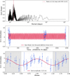 |
Fig. C.1 Top panel: GLS of the Observed-Calculated (O-C) times of transits. Middle panel: O-C times along with the best sinusoidal fitted model. Bottom panel: O-C times in phase with the best fitted period. |
Appendix D Detection sensitivity
To assess our sensitivity to planetary companions across the parameter space, we performed an injection-recovery test combining both HARPS-N RVs and the PMa. In particular, we computed the detection probability on a logarithmic grid of planetary mass (Mp sin i for RV-only, Mp for combined analysis), spanning from 10−2 MJup to 20 MJup, versus semi-major axis (a), from 10−2 au to 10 au. For each cell of the grid, we simulated 200 synthetic planetary signals. The orbital parameters were drawn as follows: the period was determined from a and the stellar mass; the time of conjunction and the argument of periastron were drawn from a uniform distribution; the orbital inclination (i) was drawn from a sinusoidal distribution (uniform in cos i); and the eccentricity was drawn from a Beta distribution, following the statistical properties of known exoplanets (Kipping 2013b).
For the RV analysis, we adopted a model comparison approach based on the BIC. For each simulated planet, we generated a synthetic RV time series at the epochs of the observed data, adding Gaussian noise scaled by the instrumental jitter (σHARPS−N) from Table B.1. We then fitted the synthetic data with three different models:
A constant model (no planet, k = 1 parameter);
A polynomial trend model (linear or quadratic, k = 2, 3) to account for long-period companions;
A full Keplerian orbit model (k = 6).
A planet was considered "detected" via RVs if the Keplerian model provided significantly better evidence than the polynomial or constant baseline models. Specifically, we required a difference ∆BIC > 10 (Kass & Raftery 1995), where BIC = χ2 + k ln(Nobs). Furthermore, planets inducing strong linear or quadratic trends (where the orbital period is significantly longer than the observational baseline) were also flagged as detected if the polynomial model was favoured over the constant model.
To evaluate the sensitivity to wide-orbit companions, we further utilized the PMa measured between the Hipparcos and Gaia eDR3 catalogues (Brandt 2018). The PMa vector corresponds to the difference between the long-term proper motion vector (approximating the centre-of-mass motion) and the short-term Gaia proper motion. We defined the astrometric detection threshold at a 3σ level. For each a, we calculated the minimum planetary mass Mmin required to induce a tangential velocity anomaly ∆vT equal to three times the measurement error ( ) reported in the HGCA. This calculation accounts for the orbital smearing effect due to the finite observing baselines of the two missions, following the formulation by Kervella et al. (2019). A simulated planet was considered astrometrically detected if its mass Mp > Mmin(a).
The final completeness map (Fig. D.1) represents the union of the two detection methods. A simulated planet in a given grid cell was considered recovered if it satisfied either the RV detection criterion (∆BIC > 10) or the PMa detection criterion (signal > 3σ). The detection fraction for each cell is defined as Ndet/Nsim. Currently, the data is sensitive to Jupiter-mass planets only up to ∼1 au.
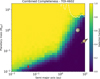 |
Fig. D.1 Detection completeness map for TOI-4602 in the mass versus semi-major axis plane, combining RV and PMa constraints. The colour scale represents the detection fraction of simulated planetary companions. The white dashed line indicates the astrometric detection limit, corresponding to a PMa signal of 3σ based on the Hipparcos-Gaia eDR3 baseline. Regions above this line are accessible via astrometry, while the inner regions are probed by RVs. The red circle marks the positions of TOI-4602 b. For context, Jupiter and Saturn are shown as icons. |
Appendix E Mass-radius diagram and internal structure: additional figures and tables
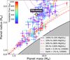 |
Fig. E.1 Mass-radius diagram of exoplanets with mass and radius derived with precision better than 20% and 10%, respectively. The colour indicates the stellar insolation in Earth units (see colour bar in the upper left corner). The mass and radius of TOI-4602 b, as derived in this work, are highlighted on the diagram. Theoretical mass-radius curves, computed assuming a surface temperature of 1000 K, are over-plotted for reference. The curve corresponding to a 20% Fe core mass fraction is taken from Zeng et al. (2016), while the remaining composition models are from Zeng et al. (2019). From top to bottom, the curves correspond to: Earth-like rocky cores (32.5% Fe + 67.5% MgSiO3) with a 0.3% and 1% H2 envelopes, and rocky compositions with varying silicates fractions (100% Fe, 33% Fe + 66% MgSiO3, 20% Fe + 80% MgSiO3, 100% MgSiO3). This plot has been generated with mr-plotter (Castro-González et al. 2023, https://github.com/castro-gzlz/mr-plotter/). |
Prior and posterior parameter distributions for the interior characterization assuming an Earth-like rocky composition.
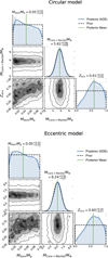 |
Fig. E.2 Marginalized posterior distribution of interior parameters in 1-D and 2-D. The shown posterior is calculated assuming an enriched H/He envelope above an Earth-like interior and is constrained by planet mass, radius, equilibrium temperature, and age. |
Appendix F Photevaporation and long-term evolution: additional figures
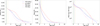 |
Fig. F.1 Temporal evolution of planetary parameters of TOI-4602 b. The left, middle and right panels show the evolution of radius, mass, and mass-loss rate, respectively. The colours refers to different high-energy evolutionary tracks as described in the text. The coloured circles indicate the planet’s current position, which depends on the age assumed in the model. In the left and middle panels, the red and blue circles coincide. Vertical dashed lines mark the limit of validity for analytical models, beyond which data are extrapolated to 10 Myr. These include the Lopez & Fortney (2014) envelope radius equation (orange), the mass loss rate ATES expression (black), and the Penz et al. (2008) X-ray luminosity equation (green) (Johnstone et al. 2021 track is valid beyond these thresholds). |
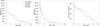 |
Fig. F.2 The same of Fig. F.1 for the enhanced metallicity composition of the planet atmosphere (see Sect. 7). |
Appendix G Atmospheric simulations: additional figures
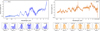 |
Fig. G.1 Simulated spectra of TOI-4602 b as observed by Ariel (left panels) and JWST (right panels). Bottom panels show the posterior distribution of the VMRs of the molecules for each simulation, respectively. The shaded areas represent the 1σ uncertainty, while the values report the media and 1σ span of the posteriors. Black dashed lines highlight the VMRs of the input model. |
The Ariel payload will consist of two instruments: the FGS providing the Fine Guidance System capabilities combined with a VIS photometer and a NIR spectrometer, and the Ariel IR Spectrometer (AIRS) providing spectra in the 1.95–7.8 µm range with a resolution of 30–100.
All Tables
TOI-4602 parameters from the transit and RV joint fit, obtained with one planet on a circular orbit model (M1 model).
Prior and posterior parameter distributions for the interior characterization assuming an Earth-like rocky composition.
All Figures
|
Fig. 1 Target pixel file from the TESS observations in Sector 43, centred on TOI-4602, which is highlighted with a white cross. The orange squares indicate the SPOC pipeline aperture, while sources from Gaia DR3 catalogue (Gaia Collaboration 2023) are overplotted with circles whose sizes are proportional to the Gaia magnitude difference with respect to our target. Grey arrows show the direction of the proper motions for all sources in the field. The colour bar indicates the electron counts per pixel. |
| In the text | |
|
Fig. 2 (Top panel) Normalized TESS PDCSAP light curves from all available sectors. The out-of-transit data have been binned to 20 minutes to improve the signal-to-noise ratio, while the in-transit data are kept at the original cadence to preserve the transit shape. Red and blue triangles mark the positions of odd and even transits, respectively. BTJD refers to the Baycentric TESS Julian Date, which is the time stamp measured in BJD and offset by 2 450 000.0. Dots in different colours represent different TESS sectors, with vertical dashed lines indicating the boundaries between them. (Bottom left panels) Odd and even transits folded using a period of 3.98 days. The consistent transit depths between odd and even transits show no evidence of alternating primary and secondary eclipses, disfavouring an eclipsing binary scenario at twice the orbital period. Black curves show smoothed light curves obtained via a moving average. (Bottom right panel) TLS periodogram of TOI 4602 b light curves. The highest peak corresponds to the main transit signal at P ≈3.98 days. The additional secondary peaks visible in the periodogram correspond to harmonics (e.g. P/2, 2P) and aliases of this primary periodicity. |
| In the text | |
|
Fig. 3 Spectroscopic time series and GLS periodogram. Left: HARPS-N spectroscopic time series analysed in this work. From top to bottom, the panels show the RVs, RV residuals, BIS, log |
| In the text | |
|
Fig. 4 Modelling of photometric and spectroscopic time series obtained from the joint fit assuming a circular model. (Left) Photometric modelling of the TOI-4602 b planetary signal. The top panel displays the normalized, phase-folded TESS transits overlaid with the best-fit model (black line), while the bottom panel shows the residuals between the observed data and the model. (Right) Phase-folded RV fit of TOI-4602 b planetary signal. The reported error bars include the jitter term, added in quadrature. The bottom panel displays the residuals of the fit. |
| In the text | |
|
Fig. 5 Evolutionary track of TOI-4602 in the effective temperature-bolometric luminosity plane. The red circle marks the current location of the star on the track. |
| In the text | |
|
Fig. 6 Time evolution of X-ray (5–100 Å), EUV (100–920 Å), and total XUV luminosity of TOI-4602, according to Penz et al. (2008) and the X-ray/EUV scaling by Sanz-Forcada et al. (2025) (red lines) and according to Johnstone et al. (2021) (blue lines). Uncertainties on the age and X-ray luminosity of TOI-4602 q(square symbol) are also indicated, with respect to the nominal value of Lx = 1027 erg/s at 6.8 Gyr. The grey area is the original locus for dG stars in Penz et al. (2008). For comparison purpose, we also show the current position of the Sun and the full range of variability during an 11-year magnetic cycle. |
| In the text | |
|
Fig. C.1 Top panel: GLS of the Observed-Calculated (O-C) times of transits. Middle panel: O-C times along with the best sinusoidal fitted model. Bottom panel: O-C times in phase with the best fitted period. |
| In the text | |
|
Fig. D.1 Detection completeness map for TOI-4602 in the mass versus semi-major axis plane, combining RV and PMa constraints. The colour scale represents the detection fraction of simulated planetary companions. The white dashed line indicates the astrometric detection limit, corresponding to a PMa signal of 3σ based on the Hipparcos-Gaia eDR3 baseline. Regions above this line are accessible via astrometry, while the inner regions are probed by RVs. The red circle marks the positions of TOI-4602 b. For context, Jupiter and Saturn are shown as icons. |
| In the text | |
|
Fig. E.1 Mass-radius diagram of exoplanets with mass and radius derived with precision better than 20% and 10%, respectively. The colour indicates the stellar insolation in Earth units (see colour bar in the upper left corner). The mass and radius of TOI-4602 b, as derived in this work, are highlighted on the diagram. Theoretical mass-radius curves, computed assuming a surface temperature of 1000 K, are over-plotted for reference. The curve corresponding to a 20% Fe core mass fraction is taken from Zeng et al. (2016), while the remaining composition models are from Zeng et al. (2019). From top to bottom, the curves correspond to: Earth-like rocky cores (32.5% Fe + 67.5% MgSiO3) with a 0.3% and 1% H2 envelopes, and rocky compositions with varying silicates fractions (100% Fe, 33% Fe + 66% MgSiO3, 20% Fe + 80% MgSiO3, 100% MgSiO3). This plot has been generated with mr-plotter (Castro-González et al. 2023, https://github.com/castro-gzlz/mr-plotter/). |
| In the text | |
|
Fig. E.2 Marginalized posterior distribution of interior parameters in 1-D and 2-D. The shown posterior is calculated assuming an enriched H/He envelope above an Earth-like interior and is constrained by planet mass, radius, equilibrium temperature, and age. |
| In the text | |
|
Fig. F.1 Temporal evolution of planetary parameters of TOI-4602 b. The left, middle and right panels show the evolution of radius, mass, and mass-loss rate, respectively. The colours refers to different high-energy evolutionary tracks as described in the text. The coloured circles indicate the planet’s current position, which depends on the age assumed in the model. In the left and middle panels, the red and blue circles coincide. Vertical dashed lines mark the limit of validity for analytical models, beyond which data are extrapolated to 10 Myr. These include the Lopez & Fortney (2014) envelope radius equation (orange), the mass loss rate ATES expression (black), and the Penz et al. (2008) X-ray luminosity equation (green) (Johnstone et al. 2021 track is valid beyond these thresholds). |
| In the text | |
|
Fig. F.2 The same of Fig. F.1 for the enhanced metallicity composition of the planet atmosphere (see Sect. 7). |
| In the text | |
|
Fig. G.1 Simulated spectra of TOI-4602 b as observed by Ariel (left panels) and JWST (right panels). Bottom panels show the posterior distribution of the VMRs of the molecules for each simulation, respectively. The shaded areas represent the 1σ uncertainty, while the values report the media and 1σ span of the posteriors. Black dashed lines highlight the VMRs of the input model. |
| In the text | |
Current usage metrics show cumulative count of Article Views (full-text article views including HTML views, PDF and ePub downloads, according to the available data) and Abstracts Views on Vision4Press platform.
Data correspond to usage on the plateform after 2015. The current usage metrics is available 48-96 hours after online publication and is updated daily on week days.
Initial download of the metrics may take a while.