| Issue |
A&A
Volume 709, May 2026
|
|
|---|---|---|
| Article Number | A205 | |
| Number of page(s) | 17 | |
| Section | Extragalactic astronomy | |
| DOI | https://doi.org/10.1051/0004-6361/202658924 | |
| Published online | 19 May 2026 | |
Transition from outside-in to inside-out at z ∼ 2: Evidence from radial profiles of the specific star formation rate based on JWST/HST
1
Department of Astronomy, University of Science and Technology of China, Hefei 230026, China
2
School of Astronomy and Space Science, University of Science and Technology of China, Hefei 230026, China
3
Institute of Deep Space Sciences, Deep Space Exploration Laboratory, Hefei 230026, China
4
School of Physics and Astronomy, Anqing Normal University, Anqing 246133, China
5
Institute of Astronomy and Astrophysics, Anqing Normal University, Anqing 246133, China
6
Key Laboratory of Modern Astronomy and Astrophysics, Nanjing University, Ministry of Education, Nanjing, Jiangsu 210093, China
7
School of Astronomy and Space Science, Nanjing University, Nanjing, Jiangsu 210093, China
8
Department of Astronomy, Tsinghua University, Beijing 100084, China
★ Corresponding authors: This email address is being protected from spambots. You need JavaScript enabled to view it.
; This email address is being protected from spambots. You need JavaScript enabled to view it.
; This email address is being protected from spambots. You need JavaScript enabled to view it.
Received:
12
January
2026
Accepted:
30
March
2026
Abstract
By combining high-resolution observations from JWST and HST, we measured the stellar masses, star formation rates (SFRs), and multiwavelength morphologies of galaxies in the CANDELS fields. Furthermore, based on rest-frame 1 μm morphologies, we derived the spatially resolved stellar mass and SFR surface density (Σ* and ΣSFR) profiles for 46,313 galaxies with reliable structural measurements at 0 < z < 4 and log(M*/M⊙) > 8, and we provide the corresponding catalog. For star-forming galaxies, our results show excellent consistency with previous studies in terms of the star formation main sequence and the size–mass relation, demonstrating the robustness of our stellar mass and SFR measurements. For spatially resolved profiles, we find that at higher redshifts (z > 2.5), the median radial profile of ΣSFR is nearly parallel to but slightly steeper than that of Σ*. This results in mildly negative gradients in the specific SFR (sSFR) profiles in all stellar mass bins we considered. These findings indicate that galaxies at z > 2.5 cannot grow in size via in situ star formation alone, challenging the understanding of galaxy size evolution beyond the cosmic noon. In contrast, at z < 2.0, the sSFR profiles transition to exhibit increasingly more positive gradients at lower redshifts, consistent with an inside-out growth scenario in which star formation preferentially expands the galactic outskirts.
Key words: galaxies: evolution / galaxies: formation / galaxies: structure
© The Authors 2026
 Open Access article, published by EDP Sciences, under the terms of the Creative Commons Attribution License (https://creativecommons.org/licenses/by/4.0), which permits unrestricted use, distribution, and reproduction in any medium, provided the original work is properly cited.
This article is published in open access under the Subscribe to Open model. This email address is being protected from spambots. You need JavaScript enabled to view it. to support open access publication.
1. Introduction
Understanding how galaxies assemble their stellar mass and grow in size over cosmic time remains a central question in galaxy formation and evolution. Over the past several decades, extensive efforts have been devoted to characterizing the growth process of galaxies, revealing that their structures form hierarchically, involving processes such as baryonic cooling, gas accretion, star formation, galaxy mergers, and a wide variety of feedback mechanisms (e.g., Cole et al. 2000; Lilly et al. 2013; Geach et al. 2014; Sánchez Almeida et al. 2014; Kacprzak 2017; Wechsler & Tinker 2018; Wang et al. 2019; Ellison et al. 2022; Davies et al. 2022; Wang & Lilly 2021, 2022b,a; Primack 2024; Ellison et al. 2024; Chen et al. 2025; Jia et al. 2025; Lyu et al. 2025).
As one of the most important aspects of galaxy growth, numerous studies have found that the majority of star formation activity occurs along the so-called star-forming main sequence (SFMS), which represents a tight correlation between stellar mass and SFR (e.g., Daddi et al. 2007; Speagle et al. 2014; Whitaker et al. 2014; Santini et al. 2017; Popesso et al. 2023; Koprowski et al. 2024; Clarke et al. 2024; Rinaldi et al. 2025; He et al. 2026). This relation exhibits a typical scatter of only about 0.3 dex, and the scatter remains nearly constant across different redshift epochs (e.g., Whitaker et al. 2012; Speagle et al. 2014; Koprowski et al. 2024), which may suggest that galaxies grow in mass over cosmic time in a state of self-regulated semiequilibrium (e.g., Daddi et al. 2010; Genzel et al. 2010; Wang et al. 2019; Tacchella et al. 2020). Additionally, many studies have demonstrated that galaxy sizes increase with stellar mass, forming the well-known size–mass relation (e.g., van der Wel et al. 2014; Mosleh et al. 2020; Nedkova et al. 2021; van der Wel et al. 2024). By combining constraints from the SFMS and the size–mass relation, some previous works have reconstructed the characteristic size–growth trajectories of individual galaxies (e.g., van Dokkum et al. 2015; Jia et al. 2024).
However, since star formation is not uniformly distributed within galaxies, studies based solely on integrated physical properties are insufficient to capture the full picture of galaxy growth. A comprehensive understanding of galaxy growth and quenching mechanisms requires not only knowledge of the integrated galaxy properties, but also their spatially resolved information (e.g., Barro et al. 2017; Jung et al. 2017; Abdurro’uf & Akiyama 2018; Wang et al. 2018; Sánchez 2020; Baker et al. 2022; Abdurro’uf et al. 2023). Spatial distributions of SFR and stellar mass provide direct insight into where growth occurs within galaxies (e.g., Nelson et al. 2012; Tacchella et al. 2015; Nelson et al. 2016; Abdurro’uf & Akiyama 2018; Tacchella et al. 2020; Abdurro’uf et al. 2023). In the low-redshift universe, spatially resolved studies have suggested that galaxies can assemble their mass in different patterns (e.g., Pérez et al. 2013; Wang et al. 2018). A minor population of galaxies exhibits rapid stellar mass assembly within their central regions. This is characterized by elevated central sSFR and relatively younger central stellar populations. This phenomenological profile corresponds to an outside-in growth mode. Conversely, most star-forming galaxies display preferential mass accumulation in their outskirts, featuring higher sSFR at large radii and comparatively older central populations. This signature is consistent with the inside-out growth scenario.
Since galaxy growth is an inherently continuous process, the increase in stellar mass (potentially along the SFMS) is accompanied by size growth and by the corresponding evolution in stellar mass surface-density and SFR surface-density profiles (e.g., Dekel et al. 2009; Tacchella et al. 2015; Nelson et al. 2016; Furlong et al. 2017; Förster Schreiber & Wuyts 2020; Jain et al. 2024; de la Vega et al. 2025). Therefore, a more complete understanding of galaxy evolution requires the combination of the integrated and spatially resolved physical properties (e.g., Hasheminia et al. 2024). For example, by analyzing the spatial profiles of stellar mass and SFR, we may predict the future size of a galaxy after a given period of star formation.
Nevertheless, the study of the spatially resolved properties of galaxies at intermediate to high redshifts critically depends on either high-quality IFS or high-resolution multiwavelength imaging. In the case of IFS, the available sample sizes are typically small and often subject to selection biases (e.g., Tacchella et al. 2015). For imaging-based approaches, most previous studies have predominantly relied on observations made with the Hubble Space Telescope (HST) (e.g., Wuyts et al. 2012; Abdurro’uf & Akiyama 2018). However, the limited wavelength coverage of the HST restricts observations to the rest-frame ultraviolet and optical at z ∼ 3, thereby hindering accurate measurements of stellar masses and other key physical properties (e.g., Ilbert et al. 2010; Song et al. 2023b; Cochrane et al. 2025). The successful launch of the James Webb Space Telescope (JWST) marks a transformative advancement, enabling more detailed investigations of resolved galaxy properties. With its deep high-resolution imaging in the near-infrared, JWST facilitates significantly more precise measurements of galaxies at intermediate to high redshifts, thereby allowing robust studies of their resolved physical structures and star formation histories (e.g., Song et al. 2023b; Cochrane et al. 2025; Mosleh et al. 2025; Harvey et al. 2025).
Some recent studies have begun to investigate the spatially resolved physical properties of galaxies by leveraging combined observations from HST and the JWST (e.g., Giménez-Arteaga et al. 2023; Abdurro’uf et al. 2023; Giménez-Arteaga et al. 2024). However, these efforts have generally been constrained by the limited availability of deep JWST observations. Over the past three observing cycles, JWST has significantly expanded its coverage by conducting deep multiband imaging across a wide range of extragalactic fields (e.g., Finkelstein et al. 2025; Eisenstein et al. 2026; Dunlop et al. 2021).
We compile JWST multiwavelength imaging from the well-established Cosmic Assembly Near-infrared Deep Extragalactic Legacy Survey (CANDELS; Grogin et al. 2011; Koekemoer et al. 2011), including observations in the Extended Groth Strip (EGS, Davis et al. 2007), the Great Observatories Origins Deep Survey South and North (GOODS-S and GOODS-N, Giavalisco et al. 2004), the Cosmic Evolution Survey (COSMOS, Scoville et al. 2007), and the UKIDSS Ultra-deep Survey (UDS, Lawrence et al. 2007), along with the existing HST observations in the same fields. Adopting a self-consistent analysis framework, we derive integrated and spatially resolved physical properties (including stellar mass and SFR) of galaxies and measure morphological parameters (e.g., half-light radius along the semimajor axis (Re), Sérsic index (n), axis ratio (q), and some nonparametric parameters) across each photometric band1 (Jia et al. 2024). As the first paper in a series, this work provides a comprehensive introduction to the method employed for deriving the integrated and spatially resolved physical properties of galaxies and for a comparison of our results with previous studies. By examining the SFMS and the size–mass relation within our galaxy sample, we find good consistency with previous studies, which validates the robustness of our analysis method. Furthermore, the investigation of spatially resolved profiles of key physical properties provides compelling evidence for the transition from outside-in to inside-out growth mode driven-by in situ star formation at redshift 2. Based on the measurements established in this study, our forthcoming work will involve the construction of galaxy samples that trace progenitor–descendant connections. These samples will be used to constrain models of galaxy growth and to study the physical mechanisms that may lead to the quenching of star formation.
This paper is organized as follows. In Section 2 we outline the data acquisition and sample selection criteria. Section 3 provides a detailed description of the method we employed to measure the integrated and spatially resolved physical properties of galaxies. The results are presented in Section 4. Section 5 discusses the possible physical mechanisms. Finally, a summary and conclusions are provided in Section 6. Throughout this paper, we adopt a flat ΛCDM cosmology with H0 = 70 km s−1 Mpc−1, Ωm = 0.3, and ΩΛ = 0.7, and a Chabrier (2003) initial mass function.
2. Data set
2.1. Multiband image
We employed JWST observations from the CANDELS fields, incorporating data from the Cosmic Evolution Early Release Science survey (CEERS, Finkelstein et al. 2025), the JWST Advanced Deep Extragalactic Survey (JADES, Eisenstein et al. 2026), and the Public Release IMaging for Extragalactic Research survey (PRIMER, Dunlop et al. 2021). The CEERS survey covers an area of 94.6 arcmin2 within the CANDELS/EGS field including JWST/NIRCam observations in the F115W, F150W, F200W, F277W, F356W, and F444W filters. The JADES survey spans 83.0 arcmin2 in the CANDELS/GOODS-N field (hereafter referred to as JADES-GDN) and 84.5 arcmin2 in the CANDELS/GOODS-S field (JADES-GDS hereafter). In addition to the same filters as in the CEERS field, JADES also includes JWST/NIRCam observations in the F090W filter. The PRIMER program covers 141.8 arcmin2 in the CANDELS/COSMOS field (PRIMER-COSMOS hereafter) and 251.2 arcmin2 in the CANDELS/UDS field (PRIMER-UDS hereafter), which uses the same broad-band filters as the JADES survey. In addition, these fields also include some medium-band observations. However, because the medium-band data are relatively shallow, we did not incorporate them into our analysis. As demonstrated in Appendix B, excluding these bands does not affect our results significantly.
All of these fields have also been observed by HST in multiple bands, including F435W, F606W, F814W, F125W, F140W, and F160W. However, given the proximity of the central wavelength of HST/F125W to that of JWST/F115W and the similarity between the central wavelengths of HST/F140W and F160W with that of JWST/F150W, we only included the F435W, F606W, and F814W filters from HST in our subsequent analysis.
The HST and JWST images were processed by the Cosmic Dawn Center (Valentino et al. 2023), and the corresponding data are publicly available through the DJA website2. The pixel scale of the final mosaic image is  /pixel. We used the most recent data releases available at the time of analysis: v7.0 for the PRIMER-COSMOS field, v7.2 for the CEERS, JADES-GDS, and PRIMER-UDS fields, and v7.3 for the JADES-GDN field.
2.2. Photometric catalog
In addition to the processed multi-wavelength imaging data, Valentino et al. (2023) also provided photometric catalogs for all available JWST and HST filters in these fields. The source detection was performed on combined images of all NIRCam long-wavelength filters (typically F277W+F356W+F444W), followed by source extraction using SEP (Barbary 2016). The photometry was measured within circular apertures with a diameter of  , with aperture corrections applied to estimate the total flux within elliptical Kron apertures. Based on these total flux measurements, photometric redshifts (zphot) were derived using EAZY-PY (Brammer et al. 2008). Additionally, spectroscopic redshift data were compiled for these fields and provided spectroscopic redshifts (zspec) for a subset of sources.
With the high quality of the HST and JWST data, Valentino et al. (2023) demonstrated that the photometric redshifts are highly reliable. By comparing zphot with zspec for the spectroscopic sample, they found normalized median absolute deviations (σNMAD) of 0.026, 0.019, 0.016, 0.022, and 0.023 for the CEERS, JADES-GDS, JADES-GDN, PRIMER-COSMOS, and PRIMER-UDS fields, respectively, where σNMAD is defined as the normalized median absolute deviation of Δz/(1 + zspec). The photometric and redshift catalogs are also publicly available on the DJA website (for further details regarding the photometric measurements and redshift estimation, we refer to Valentino et al. (2023)). We adopted the best redshifts reported by Valentino et al. (2023) and used zspec when available and zphot otherwise.
2.3. Sample selection
Numerous studies have demonstrated that point sources occupy a well-defined sequence in size–magnitude space (e.g., Skelton et al. 2014; Weaver et al. 2022). Using the half-light radius versus magnitude diagram provided in the photometric catalog, we first excluded point sources from our parent sample. To further remove potential spurious detections and sources with unreliable redshift estimates, we applied the following selection criteria to ensure a robust galaxy sample: (1) a signal-to-noise ratio (S/N) greater than 10 in the detection image (S/Ndet > 10); (2) a reduced χ2 value satisfying χ2/Nfilt ≤ 8 with at least six filters available for photometric redshift estimation (Nfilt ≥ 6), where Nfilt is the number of filters used in the fit. As we aim to estimate the physical properties of galaxies in Section 3.1, we further limited our sample to relatively bright sources by applying the following additional criteria: (3) an F444W magnitude brighter than 28.5 mag; and (4) an S/N greater than 3 in all six JWST broad bands available across all fields (F115W, F150W, F200W, F277W, F356W, and F444W), ensuring reliable spectral energy distribution (SED) fitting. These criteria yielded a final sample of 206 790 galaxies.
3. Method
3.1. The estimation of physical properties
We derived the integrated physical properties of the galaxies in our sample using the CIGALE program (Boquien et al. 2019), which is based on nine-band photometry for the CEERS field and ten-band photometry for the remaining fields. The fitting setup of CIGALE we used closely follows that of Shen et al. (2024). We first corrected the photometric catalog for the Milky Way extinction using the extinction curve of Fitzpatrick (1999) and the extinction map from Schlafly & Finkbeiner (2011). The SED fitting assumed a delayed-τ star formation history, a Bruzual & Charlot (2003) stellar population with solar metallicity, the dust attenuation law of Calzetti et al. (2000), and the nebular emission models of Inoue (2011). Mid-infrared observations were lacking, and we therefore did not include a dust emission component in our modeling.
CIGALE provided multiple estimates of SFR, including the average SFR over the past 100 Myr (SFR100 Myrs), the past 10 Myr (SFR10 Myrs), and the instantaneous SFR (SFRinstant). Unless otherwise stated, we adopted SFR100 Myrs as the representative SFR in our analysis. As discussed in Appendix B, however, the absence of F090W data in the CEERS field has a negligible effect on our estimates of stellar mass and SFR. To alleviate potential concerns regarding differences in band coverage across different survey fields, we excluded the CEERS sample from the further analysis. We examined the results after incorporating the CEERS data and found that our main conclusions remain essentially unchanged.
Figure 1 shows the redshift and stellar mass distributions of the good sample defined in Section 2.3, excluding sources from the CEERS field. Previous studies have emphasized the importance of MIRI data for accurately constraining the physical properties of galaxies at z > 4 (e.g., Papovich et al. 2023; Song et al. 2023b). However, Cochrane et al. (2025) also demonstrated that robust estimates of galaxy stellar mass can still be achieved up to z ∼ 10 using only HST and JWST/NIRCam data. In Appendix A we validate the reliability of our method in recovering galaxy physical properties at z < 4 using mock observations. To adopt a conservative approach, we limited our subsequent analysis to galaxies at z < 4, where the rest-frame ∼1 μm broad-band imaging is available. The physical properties of galaxies at higher redshifts will be investigated in future work.
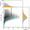 |
Fig. 1. Redshift and stellar mass distribution of our total good sample. The region enclosed by the dashed black lines indicates the selected sample we used, defined by 0 < z < 4 and log(M*/M⊙) > 8. The solid cyan curve represents the 90% stellar mass completeness limit, which corresponds to a magnitude limit of F444Wlim = 28 mag. The gray (yellow) histograms in the top and right panels show the redshift and stellar mass distributions of the good sample (selected sample), respectively. |
Given the varying depths of observations across different fields, we assessed the mass completeness of our sample by estimating the 90% completeness limit using the method described in Pozzetti et al. (2010). Based on a source-injection analysis, Merlin et al. (2024) showed that the detection rate reaches 100% for objects brighter than 28 mag in the combined F356W+F444W detection images in these fields. To ensure sample completeness, we therefore adopted a conservative magnitude limit of F444Wlim = 28 mag across all surveys we included. In each redshift bin with a width Δz = 0.25, we identified the faintest 20% of galaxies and used them to calculate the stellar mass completeness limit. Based on the typical mass-to-light ratio for each galaxy, the stellar mass limit Mlim at a given redshift slice represents the mass a galaxy would have if its apparent magnitude equaled the magnitude limit. Specifically, the stellar mass limit at a particular redshift was derived as log(Mlim) = log(M*) + 0.4(F444W − F444Wlim). Then, we defined Mcomp as the upper envelope of the Mlim distribution below which 90% of the Mlim values are located at a given redshift. We estimated the stellar mass completeness across the redshift range 0 < z < 6 and empirically parametrized it as a function of redshift: Mcomp(z) = 7.36 + 0.5ln(z). The restriction of the analysis to z < 4 does not significantly alter this result. The resulting completeness limit is shown in Figure 1. To ensure a mass-complete sample, we only included galaxies with log(M*/M⊙) > 8 and z < 4 in our subsequent analysis, which includes 67,986 galaxies in total.
3.2. PSF match
Since our goal was to perform a spatially resolved SED fitting, it was crucial to homogenize the spatial resolution across all filters. To achieve this, we selected 10–20 unsaturated point sources brighter than 24 mag in the F444W band in each field by identifying the point-source sequence in the size–magnitude diagram. Using these sources, we constructed empirical PSFs for each band with the PHOTUTILS package (Bradley et al. 2024). Then, by optimizing the performance metrics defined in Aniano et al. (2011), the PSF matching kernels were generated to match the PSF of shorter-wavelength images in each field to that of the F444W band, which has the largest full width at half maximum (FWHM is about  ). All images are then convolved with the corresponding kernels to ensure uniform spatial resolution across all bands for each field.
To visually assess the effectiveness of our PSF matching procedure, Figure 2 shows the fraction of enclosed light as a function of radius for each filter relative to the F444W band in the JADES-GDS field. The upper and lower panels show the results before and after PSF matching, respectively. As shown, after PSF matching, the encircled energy profiles of PSFs in different bands exhibit remarkable similarity, with deviations mostly within 0.01. A similar consistency is observed across all other fields, which confirms the robustness and reliability of our PSF homogenization method.
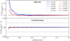 |
Fig. 2. Fraction of enclosed light as a function of radius for each filter relative to F444W in the JADES-GDS field. The upper and lower panels present the results before and after PSF matching, respectively. |
3.3. Estimating the galaxy morphology
To derive the spatially resolved physical property profiles of galaxies, we first estimated their morphologies to inform the construction of measurement apertures. We fit a single Sérsic model using GALFIT (Peng et al. 2002, 2010) to obtain key structural parameters of galaxies such as Re, n, q, and position angle (PA) for each available band (Jia et al. 2024).
Following the approach of Jia et al. (2024), we estimated the morphology at rest frame 1 μm by linearly interpolating the Sérsic parameters from the two observed bands that were nearest in wavelength. When only one suitable band was available, we directly adopted its fitted parameters. In the following analysis, the galaxy morphology refers to the morphology at rest frame 1 μm unless stated otherwise. Galaxies for which Sérsic modeling failed in both bands near rest frame 1 μm were excluded. In addition, Chen et al. (2022) demonstrated that single-Sérsic fitting with GALFIT can recover Re with an accuracy better than 20% for galaxies whose Re exceeds one-third of the PSF FWHM, while galaxies below this threshold are considered unresolved. Therefore, we also excluded sources with Re < 1 pixel (approximately one-third of the PSF FWHM) from our analysis. We also measured nonparametric morphological parameters using the statmorph_csst package (Yao et al. 2023), applied to the F444W-band images. To exclude the possible merger systems, we followed the recommendations of Conselice et al. (2003) and Conselice (2014) and remove dgalaxies with asymmetry values greater than 0.35. Finally, the morphology of 46,313 galaxies was well estimated in total.
3.4. Estimating galaxy physical property profiles
Figure 3 illustrates the procedure for deriving spatially resolved physical property profiles of our galaxy sample. For each galaxy, we extracted a 300 × 300 pixel cutout from the PSF-matched images and masked all other sources within the region. Using the galaxy center and the morphological parameters Re, q, and PA derived at rest frame 1 μm from GALFIT, we constructed a series of concentric elliptical annuli with a radial step size of 0.2Re, extending out to 5Re. Fluxes and associated uncertainties in each band were measured within these annuli using the PHOTUTILS package. Although this radial binning strategy may mix young and old stellar populations, our previous work demonstrated that in SED fitting, as long as observations at rest-frame wavelengths longer than 1 μm are included, the effect of the outshining effect is substantially reduced (Song et al. 2023b). Furthermore, to ensure consistency with our scientific objective of characterizing radial profiles of galaxy physical properties, we did not adopt other more granular binning strategies.
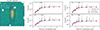 |
Fig. 3. Example of our spatially resolved SED fitting for a randomly selected galaxy. The left panel shows the F444W-band image, and the dashed black lines mark elliptical annuli spaced at intervals of 0.2Re. Four representative radial regions are highlighted in red, orange, cyan, and magenta, corresponding to 0 < r < 0.2Re, 0.4Re < r < 0.6Re, 1Re < r < 1.2Re, and 2Re < r < 2.2Re, respectively. The middle and right columns display the SED fitting results for these four radial bins. |
We then performed a spatially resolved SED fitting in each elliptical annulus using CIGALE, adopting the same configurations as described in Section 3.1. To ensure the reliability of the derived physical properties, we retained only those annuli where the S/N exceeded 3 in all six JWST broad bands, consistent with the selection criteria outlined in Section 2.3. The left panel of Figure 3 shows an example galaxy in the F444W band, with black dashed lines denoting elliptical annuli spaced at intervals of 0.2Re. The middle and right panels present the corresponding SED fitting results for four representative annuli. As illustrated, the SED fitting achieves high-quality results in annuli with sufficient S/N.
Although some studies have shown that profiles derived from PSF-matched images can be affected by PSF smearing (e.g., Szomoru et al. 2013; Suess et al. 2019; Mosleh et al. 2020; Suess et al. 2022; Miller et al. 2023) and have suggested the deconvolved images are considered more appropriate, the reliability of these deconvolution techniques has not been thoroughly assessed. Therefore, we still adopted the PSF-matched images. In Appendix C we also present results obtained from deconvolved images and find that they are nearly identical to those derived from the PSF-matched data.
4. Result
In the previous section, we have applied a self-consistent method to measure the physical properties, morphologies, and spatially resolved profiles of galaxies observed with JWST in the CANDELS fields. To prepare for the subsequent studies in this series, we use the measurements obtained in this work to investigate the SFMS, the size–mass relation, and the evolution of the physical property profiles of the galaxies.
4.1. Star formation main sequence
Over the past decade, the SFMS, including its slope, normalization, scatter, and evolution over cosmic time, has been extensively studied (e.g., Speagle et al. 2014; Leja et al. 2022; Popesso et al. 2023). These investigations have extended the characterization of the SFMS to the epoch of cosmic reionization (e.g., Clarke et al. 2024; Cole et al. 2025). Overall, the SFMS is found to follow a tight, nearly linear relation between stellar mass and SFR. However, several studies have reported a deviation from linearity at the high-mass end (e.g., M* > 1011 M⊙), commonly referred to as the bending of the SFMS (e.g., Schreiber et al. 2015; Daddi et al. 2022; Popesso et al. 2023). This trend has also recently been confirmed by early observations from Euclid (Euclid Collaboration: Enia et al. 2026).
In this study, we examine the SFMS of galaxies at z < 4 using the mass-complete sample defined in Section 3.1. The results are shown in Figure 4 with each panel presenting the results for different redshift bins. To characterize the SFMS, it is essential to separate SFGs from QGs. Bluck et al. (2024) demonstrated through simulations and observations that a threshold of sSFR < 1/tH (where tH is the Hubble time at a given redshift) reliably identifies quenched galaxies. Following this criterion, we classified galaxies with sSFR > 1/tH as star forming and included only these galaxies in our SFMS analysis. The adopted quenching threshold is shown as a gray solid line in Figure 4.
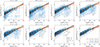 |
Fig. 4. Distribution of galaxy SFR as a function of stellar mass across different redshift bins. Each panel corresponds to a different redshift interval. The gray contours enclose 25%, 50%, 75%, and 99% of the galaxy population, respectively. The solid gray line in each panel indicates the sSFR threshold of 1/tH, where tH is the Hubble time at the median redshift of the bin; galaxies above this threshold are classified as SFGs. The black points with error bars represent the median SFR and the corresponding scatter for SFGs in different stellar mass bins. The solid black line shows the best-fit SFMS assuming the formulation in Equation (1), while the solid orange and red lines corresponds to the best-fit results derived from Equations (2) and (3), respectively. For comparison, we include results from previous studies: the dashed cyan line denotes the SFMS from Speagle et al. (2014), and the dashed orange and violet lines represent results from Popesso et al. (2023) and Koprowski et al. (2024), respectively. |
Based on a compilation of data from 25 studies, Speagle et al. (2014) explored the SFMS up to z ∼ 6 and found that for galaxies with stellar masses above 1010 M⊙, the SFMS can be well represented by a linear relation. We adopted the same functional form to describe the SFMS of our galaxy sample,
 (1)
(1)
where t represents the age of the Universe at the galaxy redshift. To model the SFMS in a way that accounts for the stellar mass and Universe age, we performed a two-dimensional fit using the Markov chain Monte Carlo (MCMC) method, implemented via the emcee package (Foreman-Mackey et al. 2013). To minimize the effect of outliers on the fitting process, we binned the galaxies by stellar mass and Universe age, as illustrated in Figure 5. The median SFR was calculated within each bin, which was then used for the fitting. In computing the likelihood function, we included the uncertainties in the median SFR for each bin, expressed as  , where σ(SFR) is the scatter in SFR within the bin and N is the number of galaxies in the bin. The best-fitting parameters are α1 = 0.745 ± 0.005, β1 = 0.0167 ± 0.001, α2 = 5.845 ± 0.042, and β2 = 0.278 ± 0.009.
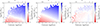 |
Fig. 5. Left panel: Distribution of SFR for SFGs mapped onto the stellar mass vs. Universe age plane, where the color scale indicates the median SFR within each square bin. Middle panel: Best-fit SFMS derived using a linear relation. Right panel: Residuals between the observed SFRs and the best-fit linear model. The small residuals demonstrate that a linear relation provides a good representation of the SFMS for our sample across the explored stellar mass and cosmic time ranges. |
The left panel of Figure 5 shows the map of galaxy SFRs in the stellar mass–Universe age plane. The middle panel displays the best-fit SFMS surface obtained from our two-dimensional fitting. The right panel illustrates the residuals between the observed median SFRs and the model predictions. As shown in the figure, this linear form of the SFMS provides a good description of our sample across the full range of stellar mass and cosmic time. The corresponding results are also shown in Figure 4. Overall, our results agree well with those of Speagle et al. (2014), except in the redshift range of 0 < z < 0.5. This discrepancy may be attributed to the different stellar mass ranges considered in the analyses and to the relatively small sample size in this redshift bin.
Moreover, several studies have reported that within the redshift range 0 < z < 3, the sSFR scales approximately as (1 + z)2.5 ∼ 3.5 (e.g., Oliver et al. 2010; Ilbert et al. 2015; Tasca et al. 2015). Motivated by this trend, some studies have also described the SFMS using the following functional form (e.g., Boogaard et al. 2018):
 (2)
(2)
We also applied this functional form to our sample and performed a two-dimensional fitting using the emcee package. The results show that this parameterization also describes the SFMS in our dataset well. The best-fit parameters are α = 0.812 ± 0.002, β = 1.811 ± 0.009, and γ = −7.762 ± 0.018. The corresponding result is shown as the orange solid line in Figure 5. As illustrated in the figure, this parameterization agrees remarkably well with the results derived using Equation (1).
Many previous studies have demonstrated that the SFMS deviates from a linear relation at the high-mass end (e.g., Schreiber et al. 2015; Daddi et al. 2022; Popesso et al. 2023; Koprowski et al. 2024). By compiling data from several studies, Popesso et al. (2023) investigated the SFMS for galaxies within the redshift range 0 < z < 6 and stellar masses between 108.5 M⊙ and 1010.5 M⊙. They found that SFR can be well described by a polynomial function of log(M*). Although the bending of the SFMS at the high-mass end is not prominent in our study because our sample includes only a few massive galaxies, we still performed a fit to our data using a polynomial function of log(M*) to capture any potential nonlinearity. We adopted the same model as Popesso et al. (2023),
 (3)
(3)
where t also represents the Universe age. Following the same procedure as described earlier, the best-fitting parameters are a0 = −0.295 ± 0.009, a1 = 0.019 ± 0.001, b0 = −9.298 ± 0.197, b1 = 1.514 ± 0.143, and b2 = −0.043 ± 0.002. The corresponding best-fit result is shown in Figure 4 as a red solid line. For comparison, we also represent the results from Popesso et al. (2023) and Koprowski et al. (2024), shown as orange and violet dashed lines, respectively.
Compared to the linear relation, this polynomial relation exhibits a slight bending at the high-mass end, which can also be seen directly from the sample distribution. When compared with the results from Popesso et al. (2023), our results are clearly consistent with theirs in the intermediate-mass range (9 < log(M*/M⊙) < 10). At the high-mass end, our result are also clearly consistent with theirs at z > 2. However, at lower redshifts, Popesso et al. (2023) revealed a more pronounced bending phenomenon. Furthermore, at the low-mass end, our results also deviate slightly when compared to those of Popesso et al. (2023). When we consider that our sample lacks massive galaxies while previous studies were deficient in low-mass galaxies, these differences can be understood reasonably well.
4.2. Size-mass relation
It is essential to understand the size growth of galaxies to uncover their evolutionary pathways because the galaxy size evolution reflects the underlying processes of mass assembly. We revisit this topic using the latest JWST observations. While many previous investigations have primarily focused on rest-frame optical sizes, it is now well studied that rest-frame optical morphologies are affected by spatial variations in stellar populations, dust attenuation, and metallicity gradients. In contrast, rest-frame near-infrared morphologies provide a more direct probe of the underlying stellar mass distribution (e.g., Suess et al. 2019; Mosleh et al. 2020; Suess et al. 2022; Miller et al. 2023; van der Wel et al. 2024; Jia et al. 2024). Therefore, we focused on the morphology of galaxies at rest-frame 1 μm to trace their stellar mass structure better.
In Figure 6 we present the size–mass relations of our SFGs sample across various redshift intervals. Following the approach of Jia et al. (2024), we modeled the dependence of the galaxy size on the stellar mass and redshift using the following functional form:
 (4)
(4)
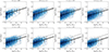 |
Fig. 6. Distribution of galaxy sizes as a function of stellar mass for SFGs across different redshift bins. In each panel, the gray contours enclose 25%, 50%, 75%, and 99% of the sample. The black points with error bars denote the median effective radius and the corresponding standard deviation within stellar mass bins. The solid black line represents the best-fit size–mass relation derived from our analysis. For comparison, we show the results for the 0 < z < 0.5 bin as dashed gray lines in the remaining panels. |
where α, β, and k are free parameters. We also performed a two-dimensional fitting using the MCMC method, adopting the same method as described in Section 4.1. Similar to Figure 5, Figure 7 presents the mapping of the median galaxy size across the stellar mass versus redshift plane. Given that at z > 3.5, only the F444W band can be used to approximate galaxy morphology at rest-frame 1μm, we restricted our analysis of the size–mass relation to galaxies at z < 3.5, where rest-frame 1μm morphologies are more reliably probed. The best-fit parameters are α = 0.164 ± 0.002, β = −0.618 ± 0.012, and k = −0.974 ± 0.017. As shown in Figure 7, the small residuals indicate that our method provides a robust characterization of the variation in galaxy size with stellar mass and redshift.
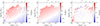 |
Fig. 7. Left panel: Distribution of size for SFGs mapped onto the stellar mass vs. redshift plane, where the color scale indicates the median size within each square bin. Middle panel: Best-fit models of the size mass relation. Right panel: Residuals between the observed size mass relation and the best-fit model. |
The size–mass relation of galaxies has also been extensively investigated in previous studies. Using data from the CANDELS fields, van der Wel et al. (2014) reported a relation of  for SFGs with stellar masses above 109 M⊙ in the redshift range 0 < z < 3, which is slightly steeper than the slope found in this work. Similar slightly steeper trends have also been observed in other studies (e.g., Mowla et al. 2019; Nedkova et al. 2021). However, based on JWST observations in the CEERS field, Ward et al. (2024) more recently reported α values ranging from 0.15 to 0.19 over 0 < z < 4, which agrees well with our results. Although these studies typically relied on rest-frame optical morphologies, which are known to be systematically larger than those measured at rest-frame 1μm (e.g., Suess et al. 2022; van der Wel et al. 2024), they nonetheless support the robustness of our measurements. In our previous work, using rest-frame 1 μm morphologies from the JADES field, Jia et al. (2024) obtained a slightly higher value of α = 0.19. This discrepancy may arise from differences in the stellar mass estimation methods.
The size evolution of SFGs offers key insights into the processes governing their growth and assembly. In previous studies, the evolution of galaxy sizes has been parameterized as re ∝ (1 + z)β, with reported values of β typically ranging from –1.3 to –0.5 (e.g., van der Wel et al. 2014; Shibuya et al. 2015; Song et al. 2023a; Ward et al. 2024; Ormerod et al. 2024; Varadaraj et al. 2024; Yang et al. 2025). For instance, using HST data from the CANDELS fields, van der Wel et al. (2014) found β ≈ −0.75 for late-type galaxies. More recently, JWST-based analyses of CEERS data yielded β = −0.63 by Ward et al. (2024), and β = −0.71 by Ormerod et al. (2024). Our own best-fit value of β = −0.618 ± 0.012 agrees well with these findings, which may suggests that galaxy morphologies in the near-infrared exhibit evolutionary trends similar to those observed in the optical bands. To illustrate the redshift evolution of galaxy size derived from our sample more clearly, we took galaxies with stellar mass ∼5 × 10¹⁰ M⊙ as a representative example to illustrate the evolutionary trend of our sample. This is shown in Figure 8. To facilitate comparison with previous studies, we also show the corresponding results from van der Wel et al. (2014), based on galaxy sizes measured at rest-frame 0.5 μm, and from Martorano et al. (2024), derived from rest-frame 1.5 μm size measurements. They clearly exhibit similar evolutionary trends, albeit with some systematic offsets. However, this is reasonable given that numerous studies have shown that galaxy sizes measured at longer wavelengths are systematically smaller than those derived at shorter wavelengths (e.g., Jia et al. 2024; McGrath et al. 2026). A more comprehensive exploration of the differences between rest-frame optical and near-infrared morphologies, including their redshift and stellar mass dependencies, will be presented in a forthcoming study.
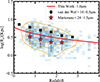 |
Fig. 8. Two-dimensional histogram (blue) of the galaxy distribution with stellar mass ∼5 × 10¹⁰ M⊙. The orange contours enclose 25%, 50%, and 75% of the sample. The solid red line indicates the best-fitting relation derived in Section 4.2. To facilitate comparison with previous studies, the results from van der van der Wel et al. (2014), derived from rest-frame 0.5 μm sizes, are shown as black squares, and those from Martorano et al. (2024), derived from rest-frame 1.5 μm sizes, are shown as red stars. |
4.3. Stellar mass profile
To investigate the dependence of the physical property profiles of the galaxies on redshift and stellar mass, we divided our sample into three stellar mass bins (108 ∼ 109 M⊙, 109 ∼ 1010 M⊙, and 1010 ∼ 1012 M⊙) and eight redshift bins (with an interval of Δz = 0.5). For each galaxy, we adopted the same S/N criterion as in Section 2.3 to ensure the reliability of measurements: only annuli with S/N exceeding 3 in all six JWST bands were retained. We defined the quantity max_high_snr_radius as the largest radius within which this criterion is satisfied. For each redshift–stellar mass bin, we derived the median physical property profile by computing the median surface density of the relevant quantity across all galaxies at each radius. If the radius under consideration exceeded max_high_snr_radius of a galaxy, we linearly extrapolated that galaxy profile to estimate its physical property at that radius. To maintain robustness, we restricted our analysis to the radial range within which more than 50% of the galaxy max_high_snr_radii exceeded this limit.
Figure 9 presents the Σ* profiles of our sample. In each panel, different colors represent results from different redshift bins. The first and second rows display the profiles as a function of radius normalized by Re and in physical units (kpc), respectively. The shaded regions in the first row represent the 25th–75th percentile distribution of Σ* at different radius. In addition, we have also estimated the standard error of Σ* at each radius to quantify the uncertainties in our radial profiles, which are typically smaller than 0.05 dex. Since the Σ* profiles in kpc units are close across different redshifts, we have opted not to include the corresponding shaded regions for better visualization. Since many previous works demonstrated that radial profiles within radii smaller than the PSF FWHM are strongly affected by PSF smearing (e.g., Liu et al. 2018; Hasheminia et al. 2024), we also show the extent of the PSF FWHM using a shaded gray region in the bottom panel. For results in physical units, we also performed a linear extrapolation of the outer profiles, which is shown as a dashed line, to infer the stellar mass surface density in the outskirts of galaxies.
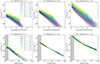 |
Fig. 9. Radial profiles of stellar mass surface density for SFGs, categorized into three stellar mass intervals and eight redshift intervals. For each bin, we present the median Σ* as a function of radius, normalized by the Re (top row) and in physical units of kiloparsec (bottom row). To ensure the reliability of the profiles, we limit the radial range to regions where more than 50% of galaxies in the bin satisfy the adopted criterion for the signal-to-noise ratio. The shaded regions in the top panels denote the 25th–75th percentile distribution of Σ* at each radius. Due to the close of the profiles in physical units across different redshifts, we omit the corresponding distribution in the bottom panels for clarity. We also show the extent of the PSF FWHM using a shaded gray region in the bottom panel. For results in physical units, we also performed a linear extrapolation of the outer profiles, which is shown as a dashed line, to infer the stellar mass surface density in the galaxy outskirts. |
As shown in Figure 9, the Σ* profiles exhibit clear negative gradients across all redshift and stellar mass bins, with Σ* decreasing as a function of radius. This results has also been reported in many previous studies (e.g., Nelson et al. 2016; Abdurro’uf & Akiyama 2018; Mosleh et al. 2020; Nelson et al. 2021; Abdurro’uf et al. 2023; Miller et al. 2023; van der Wel et al. 2024; Hasheminia et al. 2024; de la Vega et al. 2025). At fixed redshift, more massive systems consistently exhibit higher Σ*, even in their central regions. This trend is consistent with many previous findings (e.g., Abdurro’uf et al. 2023; Hasheminia et al. 2024; de la Vega et al. 2025). This pattern implies that during the course of star formation, galaxies progressively build up their central stellar mass. These results provide important constraints on galaxy growth models, such as that proposed by Nelson et al. (2016), which suggests that galaxies form compact cores at early epochs and subsequently grow their outer regions over time. However, it is important to emphasize that our current analysis focuses solely on the variation of Σ* as a function of redshift and stellar mass and does not directly trace individual evolutionary pathways. In future work, we aim to construct more carefully selected samples that might allow us to identify progenitor–descendant connections, thereby enabling a more direct investigation of galaxy growth mechanisms.
For galaxies at a fixed stellar mass, galaxies at higher redshifts tend to have higher Σ* values, which is consistent with the expectation that galaxies at earlier cosmic times are generally more compact. Similar trends have been reported in the literature (e.g., Barro et al. 2017; Jung et al. 2017). Using HST observations, Barro et al. (2017) found that galaxies with M* ∼ 109 M⊙ show a decline of approximately 0.3 dex in central stellar mass surface density within 1 kpc from z ∼ 3 to z ∼ 0.5, which agrees with our results. However, the underlying physical mechanisms that cause the increased compactness of high-redshift galaxies remain uncertain.
4.4. SFR and sSFR profile evolution
The stellar mass of a galaxy reflects the cumulative result of its past star formation activities. In this section, we investigate the recent star formation activity of galaxies by examining their ΣSFR and sSFR (defined as ΣSFR/Σ*) profiles, shown in Figure 10 and Figure 11. As shown in Figure 10, the ΣSFR profiles exhibit negative gradients across all redshift and stellar mass bins, with a flattening trend observed in the central regions. Many studies have highlighted the existence of a resolved SFMS (rSFMS), that is, of a tight correlation between the SFR surface density and the stellar mass surface density (e.g., Lin et al. 2019; Baker et al. 2022). The negative ΣSFR profiles observed here can be naturally explained by this rSFMS, in conjunction with the negative gradient of the stellar mass profile.
When we compare the ΣSFR profiles of galaxies at different redshifts, we observe that higher-redshift galaxies exhibit elevated ΣSFR across all radii. This trend likely reflects the higher gas fractions or increased cold gas accretion rates that are characteristic of galaxies at earlier cosmic times. For the dependence on stellar mass, galaxies with higher stellar masses consistently show higher ΣSFR at all radii than their lower-mass counterparts. This is expected because more massive galaxies have higher Σ* at all radii, which agrees with the existence of the rSFMS. Several studies suggested that the integrated SFMS arises from the underlying rSFMS, indicating that the relation between Σ* and ΣSFR is more fundamental. In future work, we will further investigate the connection between the resolved and integrated SFMS using the spatially resolved physical properties derived in this study.
For the sSFR profiles, we found a distinct behavior across different redshift ranges. As shown in Figure 11, for galaxies at z < 2, we observe a positive sSFR gradient, and this trend becomes more pronounced in more massive galaxies. This trend has been observed in many previous studies (e.g., Nelson et al. 2016; Morselli et al. 2019; Shen et al. 2024; Hasheminia et al. 2024). Galaxies across all redshift and stellar mass bins exhibit negative ΣSFR gradients, and the observed positive sSFR gradients therefore reflect an inside-out growth scenario. In contrast, for galaxies at z > 2.5, there is a negative sSFR gradient, although it is less pronounced for more massive galaxies. To quantitatively characterize the sSFR gradient, we measured the sSFR gradient between 0.5Re and 2.5Re. We chose this radial range to ensure that the separation was larger than the PSF FWHM, thereby minimizing the effect of PSF smearing. At the same time, this range allowed us to estimate sSFR gradients consistently across different mass bins. Similar to Σ*, we also estimated the standard error at each radius to characterize the uncertainties in the sSFR profile, and we subsequently determined the corresponding errors in the inferred gradients. Additionally, using physical units, we evaluated the sSFR gradients between 0.5 kpc and 2.5 kpc. The results are summarized in Table 1. As indicated in the table, galaxies with log(M*/M⊙) < 10 are significant shifted from positive sSFR gradients at z < 2 to negative gradients at z > 2.5. Massive galaxies show a qualitatively similar trend, but the associated uncertainties are substantially larger because the number of high-redshift massive galaxies is limited. Additionally, since high-redshift star formation is more stochastic, we examined whether a shorter timescale (10 Myr) for the SFR tracer would provide different results, but the results remained unchanged.
sSFR gradient at different stellar masses and redshift bins.
While positive sSFR gradients at z < 2 have been reported in numerous studies, however, results at higher redshifts, particularly for low-mass galaxies, have not been systematically investigated prior to JWST. Using data from the VELA simulation (Ceverino et al. 2014; Zolotov et al. 2015), Tacchella et al. (2016) demonstrated that galaxies begin to exhibit positive sSFR gradients at redshifts below z ∼ 3. By combining HST and JWST data, Abdurro’uf et al. (2023) studied the sSFR profiles of 219 SFGs and found that the sSFR radial profiles of the majority of galaxies at z > 2.5 are broadly flat. In a recent study based on JWST slitless data, Matharu et al. (2024) reported that galaxies at 4.8 < z < 6.5 exhibit roughly positive EW(Hα), which may indicate a positive sSFR gradient. However, in another study using data from the JADES field, Tripodi et al. (2024) found that galaxies at z > 4 exhibit negative EW(Hβ) profiles, which implies a negative sSFR gradient at this redshift range. Using a sample of 669 galaxies at 4 < z < 8 in the CEERS field, Jin et al. (2025) found in contrast that high-redshift galaxies predominantly exhibit positive color gradients, which also indicates centrally concentrated star formation. These findings are consistent with the results presented in our work. However, the physical mechanisms driving this transition and the dependence on stellar mass remain unclear and warrant further investigation.
Moreover, since sSFR measures the ratio of recently formed stellar mass to the total stellar mass, a positive sSFR gradient indicates that the outskirts of galaxies are growing more rapidly in stellar mass, which might expand their overall size. On the other hand, a negative sSFR gradient would indicate more efficient stellar mass buildup in the central regions, which may lead to a more compact morphology. The transition from a negative to a positive sSFR gradient may lead to a different size growth status. At lower redshifts, star formation contributes significantly to galaxy size growth, particularly for high-mass systems. In contrast, at higher redshifts, the role of in situ star formation in driving size growth appears to be less prominent or even result in a smaller effective radius. If this trend continues to even higher redshifts, it might lead to a negative size–mass relation, which has already been found in observations (e.g., Ormerod et al. 2024) and some cosmological simulations (e.g., Genel et al. 2018; Costantin et al. 2023). A more thorough and comprehensive investigation may be needed to understand the results at higher redshifts.
5. Discussion
Our analysis of the spatially resolved sSFR profiles revealed a pivotal transition in the mode of galaxy assembly around z ∼ 2. Specifically, the shift from negative sSFR gradients at high redshifts (z > 2.5) to positive gradients at lower redshifts (z < 2) suggests a fundamental change in the way star-forming galaxies acquire gas and build their stellar mass. The observed evolution may reflect the interplay between the angular momentum of accreting gas, the dynamical stability of galactic disks, and feedback processes that regulate star formation.
The prevalence of negative sSFR gradients observed in our sample at z > 2.5 points to a phase in which mass assembly is centrally concentrated. In the high-redshift Universe, the accretion of cold gas streams is characterized by relatively low specific angular momentum (e.g., Pichon et al. 2011; Dubois et al. 2012). When combined with violent disk instabilities prevalent in these highly gas-rich and turbulent disks, gas clumps lose angular momentum rapidly and migrate inward toward the galaxy center (e.g., Zolotov et al. 2015; Dekel et al. 2020). This efficient funneling of gas triggers intense nuclear starbursts, naturally resulting in the negative sSFR gradients we observe, where the specific star formation rate is significantly higher in the core than in the outskirts. As new stellar mass is preferentially added to the central region, the galaxy mass distribution becomes highly concentrated.
At z < 2, the emergence of positive sSFR gradients signals a transition to the classical inside-out growth mode. Several physical processes can conspire to drive this shift. First, as the assembled central bulge becomes sufficiently massive, it deepens the central potential and stabilizes the inner disk against further violent inflows (e.g., Martig et al. 2009). Simultaneously, the nature of gas accretion evolves with cosmic time. Cosmological models dictate that subsequent gas accretion onto the dark matter halo carries significantly higher specific angular momentum due to the expansion of the Universe and the growth of the halo virial radius (e.g., Pichon et al. 2011; Stewart 2017). This high-angular-momentum gas cannot penetrate the deep central potential well; instead, it settles into an extended disk structure in the galaxy outskirts (Obreschkow & Glazebrook 2014). Consequently, star formation becomes most active in these outer regions, resulting in the positive sSFR gradients observed in our lower-redshift sample. This marks the onset of secular disk growth, where the continuous addition of mass at large radii leads to the gradual buildup of a stellar envelope and a steady increase in the effective galaxy size.
6. Summary
By combining high-resolution imaging data from JWST and HST, we have measured the integrated and spatially resolved physical properties of galaxies with log(M*/M⊙) > 8 over the redshift range 0 < z < 4 in the CANDELS fields. This work is the first in our series of studies. By investigating the relationships between galaxy-integrated and spatially resolved physical properties, we here draw the following conclusions:
(1) For galaxies at z < 4, combining HST and JWST data allows us to reliably recover the stellar mass and SFRs. Additionally, within the range log(M*/M⊙) > 8, the star-forming main sequence of galaxies exhibits a roughly linear relation.
(2) Regarding the morphologies of galaxies in the rest-frame 1 μm band, the size-mass relation and size evolution of galaxies show trends similar to those in optical bands, following the relation  .
.
(3) By comparing the physical property profiles across different redshift and stellar mass bins, we found that across all redshift and stellar mass ranges, galaxies consistently exhibit negative gradients in the stellar mass surface density and SFR surface density. Furthermore, at higher redshifts and stellar masses, galaxies tend to show higher stellar mass and SFR surface densities.
(4) For the sSFR profiles, we observed a distinct trend: at z > 2.5, galaxies display a mild negative gradient in sSFR profiles, whereas at lower redshifts, they exhibit a positive gradient. These findings suggest that galaxies undergo a transition in their stellar assembly mode that is driven by in situ star formation and shifts them from an outside-in to an inside-out growth pattern at z ∼ 2. This marks a pivotal shift in their structural evolution. This finding deepens the mystery of how galaxies grow in size beyond the cosmic noon. More research is required to resolve the puzzle.
Data availability
The data are available at the CDS via https://cdsarc.cds.unistra.fr/viz-bin/cat/J/A+A/709/A205
Acknowledgments
This work is supported by the National Science Foundation of China (NSFC, Grant No. 12233008, No. 12473008), the National Key R&D Program of China (2023YFA1608100), the Strategic Priority Research Program of the Chinese Academy of Sciences (Grant No. XDB0550200), the Cyrus Chun Ying Tang Foundations, and the 111 Project for “Observational and Theoretical Research on Dark Matter and Dark Energy” (B23042), and the Start-up Fund of the University of Science and Technology of China (No. KY2030000200). The data products presented herein were retrieved from the Dawn JWST Archive (DJA). DJA is an initiative of the Cosmic Dawn Center (DAWN), which is funded by the Danish National Research Foundation under grant DNRF140. This work is based on observations made with the NASA/ESA/CSA James Webb Space Telescope. The data were obtained from the Mikulski Archive for Space Telescopes at the Space Telescope Science Institute, which is operated by the Association of Universities for Research in Astronomy, Inc., under NASA contract NAS 5-03127 for JWST. The data described here can be obtained from https://dx.doi.org/10.17909/z7p0-8481, https://dx.doi.org/10.17909/8tdj-8n28, and https://dx.doi.org/10.17909/T94S3X.
References
- Abdurro’uf, & Akiyama, M. 2018, MNRAS, 479, 5083 [CrossRef] [Google Scholar]
- Abdurro’uf, Coe, D., Jung, I., et al. 2023, ApJ, 945, 117 [CrossRef] [Google Scholar]
- Aniano, G., Draine, B. T., Gordon, K. D., & Sandstrom, K. 2011, PASP, 123, 1218 [Google Scholar]
- Baker, W. M., Maiolino, R., Bluck, A. F. L., et al. 2022, MNRAS, 510, 3622 [NASA ADS] [CrossRef] [Google Scholar]
- Barbary, K. 2016, J. Open Source Software, 1, 58 [NASA ADS] [CrossRef] [Google Scholar]
- Barro, G., Faber, S. M., Koo, D. C., et al. 2017, ApJ, 840, 47 [Google Scholar]
- Bluck, A. F. L., Conselice, C. J., Ormerod, K., et al. 2024, ApJ, 961, 163 [Google Scholar]
- Boogaard, L. A., Brinchmann, J., Bouché, N., et al. 2018, A&A, 619, A27 [NASA ADS] [CrossRef] [EDP Sciences] [Google Scholar]
- Boquien, M., Burgarella, D., Roehlly, Y., et al. 2019, A&A, 622, A103 [NASA ADS] [CrossRef] [EDP Sciences] [Google Scholar]
- Bradley, L., Sipőcz, B., Robitaille, T., et al. 2024, https://doi.org/10.5281/zenodo.13989456 [Google Scholar]
- Brammer, G. B., van Dokkum, P. G., & Coppi, P. 2008, ApJ, 686, 1503 [Google Scholar]
- Bruzual, G., & Charlot, S. 2003, MNRAS, 344, 1000 [NASA ADS] [CrossRef] [Google Scholar]
- Calzetti, D., Armus, L., Bohlin, R. C., et al. 2000, ApJ, 533, 682 [NASA ADS] [CrossRef] [Google Scholar]
- Ceverino, D., Klypin, A., Klimek, E. S., et al. 2014, MNRAS, 442, 1545 [NASA ADS] [CrossRef] [Google Scholar]
- Chabrier, G. 2003, PASP, 115, 763 [Google Scholar]
- Chen, G., Zhang, H.-X., Kong, X., et al. 2022, ApJ, 934, L35 [Google Scholar]
- Chen, Z., Wang, E., Zou, H., et al. 2025, ApJ, 981, 81 [Google Scholar]
- Clarke, L., Shapley, A. E., Sanders, R. L., et al. 2024, ApJ, 977, 133 [NASA ADS] [CrossRef] [Google Scholar]
- Cochrane, R. K., Katz, H., Begley, R., Hayward, C. C., & Best, P. N. 2025, ApJ, 978, L42 [Google Scholar]
- Cole, S., Lacey, C. G., Baugh, C. M., & Frenk, C. S. 2000, MNRAS, 319, 168 [Google Scholar]
- Cole, J. W., Papovich, C., Finkelstein, S. L., et al. 2025, ApJ, 979, 193 [Google Scholar]
- Conselice, C. J. 2014, ARA&A, 52, 291 [CrossRef] [Google Scholar]
- Conselice, C. J., Bershady, M. A., Dickinson, M., & Papovich, C. 2003, AJ, 126, 1183 [CrossRef] [Google Scholar]
- Costantin, L., Pérez-González, P. G., Vega-Ferrero, J., et al. 2023, ApJ, 946, 71 [NASA ADS] [CrossRef] [Google Scholar]
- Daddi, E., Dickinson, M., Morrison, G., et al. 2007, ApJ, 670, 156 [NASA ADS] [CrossRef] [Google Scholar]
- Daddi, E., Bournaud, F., Walter, F., et al. 2010, ApJ, 713, 686 [NASA ADS] [CrossRef] [Google Scholar]
- Daddi, E., Delvecchio, I., Dimauro, P., et al. 2022, A&A, 661, L7 [NASA ADS] [CrossRef] [EDP Sciences] [Google Scholar]
- Davies, J. J., Pontzen, A., & Crain, R. A. 2022, MNRAS, 515, 1430 [CrossRef] [Google Scholar]
- Davis, M., Guhathakurta, P., Konidaris, N. P., et al. 2007, ApJ, 660, L1 [NASA ADS] [CrossRef] [Google Scholar]
- Davis, K., Trump, J. R., Simons, R. C., et al. 2024, ApJ, 974, 42 [NASA ADS] [CrossRef] [Google Scholar]
- de la Vega, A., Kassin, S. A., Pacifici, C., et al. 2025, ApJ, 980, 168 [Google Scholar]
- Dekel, A., Birnboim, Y., Engel, G., et al. 2009, Nature, 457, 451 [Google Scholar]
- Dekel, A., Ginzburg, O., Jiang, F., et al. 2020, MNRAS, 493, 4126 [CrossRef] [Google Scholar]
- Dubois, Y., Pichon, C., Haehnelt, M., et al. 2012, MNRAS, 423, 3616 [NASA ADS] [CrossRef] [Google Scholar]
- Dunlop, J. S., Abraham, R. G., Ashby, M. L. N., et al. 2021, PRIMER: Public Release IMaging for Extragalactic Research, JWST Proposal. Cycle 1, ID. 1837 [Google Scholar]
- Eisenstein, D. J., Willott, C., Alberts, S., et al. 2026, ApJS, 283, 6 [Google Scholar]
- Ellison, S. L., Wilkinson, S., Woo, J., et al. 2022, MNRAS, 517, L92 [NASA ADS] [CrossRef] [Google Scholar]
- Ellison, S., Ferreira, L., Wild, V., et al. 2024, Open J. Astrophys., 7, 121 [Google Scholar]
- Euclid Collaboration (Enia, A., et al.) 2026, A&A, in press, https://doi.org/10.1051/0004-6361/202554576 [Google Scholar]
- Finkelstein, S. L., Bagley, M. B., Arrabal Haro, P., et al. 2025, ApJ, 983, L4 [Google Scholar]
- Fitzpatrick, E. L. 1999, PASP, 111, 63 [Google Scholar]
- Foreman-Mackey, D., Hogg, D. W., Lang, D., & Goodman, J. 2013, PASP, 125, 306 [Google Scholar]
- Förster Schreiber, N. M., & Wuyts, S. 2020, ARA&A, 58, 661 [Google Scholar]
- Furlong, M., Bower, R. G., Crain, R. A., et al. 2017, MNRAS, 465, 722 [Google Scholar]
- Geach, J. E., Hickox, R. C., Diamond-Stanic, A. M., et al. 2014, Nature, 516, 68 [NASA ADS] [CrossRef] [Google Scholar]
- Genel, S., Nelson, D., Pillepich, A., et al. 2018, MNRAS, 474, 3976 [Google Scholar]
- Genzel, R., Tacconi, L. J., Gracia-Carpio, J., et al. 2010, MNRAS, 407, 2091 [NASA ADS] [CrossRef] [Google Scholar]
- Giavalisco, M., Ferguson, H. C., Koekemoer, A. M., et al. 2004, ApJ, 600, L93 [NASA ADS] [CrossRef] [Google Scholar]
- Giménez-Arteaga, C., Oesch, P. A., Brammer, G. B., et al. 2023, ApJ, 948, 126 [CrossRef] [Google Scholar]
- Giménez-Arteaga, C., Fujimoto, S., Valentino, F., et al. 2024, A&A, 686, A63 [NASA ADS] [CrossRef] [EDP Sciences] [Google Scholar]
- Grogin, N. A., Kocevski, D. D., Faber, S. M., et al. 2011, ApJS, 197, 35 [NASA ADS] [CrossRef] [Google Scholar]
- Harvey, T., Conselice, C. J., Adams, N. J., et al. 2025, MNRAS, 542, 2998 [Google Scholar]
- Hasheminia, M., Mosleh, M., Hosseini-ShahiSavandi, S. Z., & Tacchella, S. 2024, ApJ, 975, 252 [Google Scholar]
- He, Z., Wang, E., Ho, L. C., et al. 2026, MNRAS, 547, 11 [Google Scholar]
- Ilbert, O., Salvato, M., Le Floc’h, E., et al. 2010, ApJ, 709, 644 [Google Scholar]
- Ilbert, O., Arnouts, S., Le Floc’h, E., et al. 2015, A&A, 579, A2 [NASA ADS] [CrossRef] [EDP Sciences] [Google Scholar]
- Inoue, A. K. 2011, MNRAS, 415, 2920 [NASA ADS] [CrossRef] [Google Scholar]
- Jain, S., Tacchella, S., & Mosleh, M. 2024, Open J. Astrophys., 7, 113 [Google Scholar]
- Jia, C., Wang, E., Wang, H., et al. 2024, ApJ, 977, 165 [Google Scholar]
- Jia, C., Wang, E., Lyu, C., et al. 2025, ApJ, 986, L24 [Google Scholar]
- Jin, B., Ho, L. C., & Sun, W. 2025, ApJ, 993, 225 [Google Scholar]
- Jung, I., Finkelstein, S. L., Song, M., et al. 2017, ApJ, 834, 81 [Google Scholar]
- Kacprzak, G. G. 2017, Astrophys. Space Sci. Libr., 430, 145 [Google Scholar]
- Koekemoer, A. M., Faber, S. M., Ferguson, H. C., et al. 2011, ApJS, 197, 36 [NASA ADS] [CrossRef] [Google Scholar]
- Koprowski, M. P., Wijesekera, J. V., Dunlop, J. S., et al. 2024, A&A, 691, A164 [NASA ADS] [CrossRef] [EDP Sciences] [Google Scholar]
- Lawrence, A., Warren, S. J., Almaini, O., et al. 2007, MNRAS, 379, 1599 [Google Scholar]
- Leja, J., Speagle, J. S., Ting, Y.-S., et al. 2022, ApJ, 936, 165 [NASA ADS] [CrossRef] [Google Scholar]
- Lilly, S. J., Carollo, C. M., Pipino, A., Renzini, A., & Peng, Y. 2013, ApJ, 772, 119 [NASA ADS] [CrossRef] [Google Scholar]
- Lin, L., Pan, H.-A., Ellison, S. L., et al. 2019, ApJ, 884, L33 [NASA ADS] [CrossRef] [Google Scholar]
- Liu, F. S., Jia, M., Yesuf, H. M., et al. 2018, ApJ, 860, 60 [NASA ADS] [CrossRef] [Google Scholar]
- Lyu, C., Wang, E., Zhang, H., et al. 2025, ApJ, 981, L6 [Google Scholar]
- Martig, M., Bournaud, F., Teyssier, R., & Dekel, A. 2009, ApJ, 707, 250 [Google Scholar]
- Martorano, M., van der Wel, A., Baes, M., et al. 2024, ApJ, 972, 134 [Google Scholar]
- Matharu, J., Nelson, E. J., Brammer, G., et al. 2024, A&A, 690, A64 [NASA ADS] [CrossRef] [EDP Sciences] [Google Scholar]
- McGrath, E. J., Finkelstein, S. L., Barro, G., et al. 2026, ApJ, 999, L6 [Google Scholar]
- Merlin, E., Santini, P., Paris, D., et al. 2024, A&A, 691, A240 [NASA ADS] [CrossRef] [EDP Sciences] [Google Scholar]
- Miller, T. B., van Dokkum, P., & Mowla, L. 2023, ApJ, 945, 155 [NASA ADS] [CrossRef] [Google Scholar]
- Morselli, L., Popesso, P., Cibinel, A., et al. 2019, A&A, 626, A61 [NASA ADS] [CrossRef] [EDP Sciences] [Google Scholar]
- Mosleh, M., Hosseinnejad, S., Hosseini-ShahiSavandi, S. Z., & Tacchella, S. 2020, ApJ, 905, 170 [NASA ADS] [CrossRef] [Google Scholar]
- Mosleh, M., Riahi-Zamin, M., & Tacchella, S. 2025, ArXiv e-prints [arXiv:2503.14591] [Google Scholar]
- Mowla, L. A., van Dokkum, P., Brammer, G. B., et al. 2019, ApJ, 880, 57 [NASA ADS] [CrossRef] [Google Scholar]
- Nedkova, K. V., Häußler, B., Marchesini, D., et al. 2021, MNRAS, 506, 928 [NASA ADS] [CrossRef] [Google Scholar]
- Nelson, E. J., van Dokkum, P. G., Brammer, G., et al. 2012, ApJ, 747, L28 [CrossRef] [Google Scholar]
- Nelson, E. J., van Dokkum, P. G., Förster Schreiber, N. M., et al. 2016, ApJ, 828, 27 [Google Scholar]
- Nelson, E. J., Tacchella, S., Diemer, B., et al. 2021, MNRAS, 508, 219 [NASA ADS] [CrossRef] [Google Scholar]
- Obreschkow, D., & Glazebrook, K. 2014, ApJ, 784, 26 [Google Scholar]
- Oliver, S., Frost, M., Farrah, D., et al. 2010, MNRAS, 405, 2279 [NASA ADS] [Google Scholar]
- Ormerod, K., Conselice, C. J., Adams, N. J., et al. 2024, MNRAS, 527, 6110 [Google Scholar]
- Papovich, C., Cole, J. W., Yang, G., et al. 2023, ApJ, 949, L18 [NASA ADS] [CrossRef] [Google Scholar]
- Peng, C. Y., Ho, L. C., Impey, C. D., & Rix, H.-W. 2002, AJ, 124, 266 [Google Scholar]
- Peng, C. Y., Ho, L. C., Impey, C. D., & Rix, H.-W. 2010, AJ, 139, 2097 [Google Scholar]
- Pérez, E., Cid Fernandes, R., González Delgado, R. M., et al. 2013, ApJ, 764, L1 [Google Scholar]
- Pichon, C., Pogosyan, D., Kimm, T., et al. 2011, MNRAS, 418, 2493 [CrossRef] [Google Scholar]
- Popesso, P., Concas, A., Cresci, G., et al. 2023, MNRAS, 519, 1526 [Google Scholar]
- Pozzetti, L., Bolzonella, M., Zucca, E., et al. 2010, A&A, 523, A13 [NASA ADS] [CrossRef] [EDP Sciences] [Google Scholar]
- Primack, J. R. 2024, Ann. Rev. Nucl. Part. Sci., 74, 173 [Google Scholar]
- Rinaldi, P., Navarro-Carrera, R., Caputi, K. I., et al. 2025, ApJ, 981, 161 [Google Scholar]
- Sánchez Almeida, J., Elmegreen, B. G., Muñoz-Tuñón, C., & Elmegreen, D. M. 2014, A&ARv, 22, 71 [Google Scholar]
- Sánchez, S. F. 2020, ARA&A, 58, 99 [Google Scholar]
- Santini, P., Fontana, A., Castellano, M., et al. 2017, ApJ, 847, 76 [NASA ADS] [CrossRef] [Google Scholar]
- Schlafly, E. F., & Finkbeiner, D. P. 2011, ApJ, 737, 103 [Google Scholar]
- Schreiber, C., Pannella, M., Elbaz, D., et al. 2015, A&A, 575, A74 [NASA ADS] [CrossRef] [EDP Sciences] [Google Scholar]
- Scoville, N., Aussel, H., Brusa, M., et al. 2007, ApJS, 172, 1 [Google Scholar]
- Shen, L., Papovich, C., Matharu, J., et al. 2024, ApJ, 963, L49 [NASA ADS] [CrossRef] [Google Scholar]
- Shibuya, T., Ouchi, M., & Harikane, Y. 2015, ApJS, 219, 15 [Google Scholar]
- Skelton, R. E., Whitaker, K. E., Momcheva, I. G., et al. 2014, ApJS, 214, 24 [Google Scholar]
- Song, J., Fang, G., Gu, Y., Lin, Z., & Kong, X. 2023a, ApJ, 950, 130 [NASA ADS] [CrossRef] [Google Scholar]
- Song, J., Fang, G., Lin, Z., Gu, Y., & Kong, X. 2023b, ApJ, 958, 82 [NASA ADS] [CrossRef] [Google Scholar]
- Speagle, J. S., Steinhardt, C. L., Capak, P. L., & Silverman, J. D. 2014, ApJS, 214, 15 [Google Scholar]
- Stewart, K. R. 2017, Astrophys. Space Sci. Libr., 430, 249 [Google Scholar]
- Suess, K. A., Kriek, M., Price, S. H., & Barro, G. 2019, ApJ, 877, 103 [NASA ADS] [CrossRef] [Google Scholar]
- Suess, K. A., Bezanson, R., Nelson, E. J., et al. 2022, ApJ, 937, L33 [NASA ADS] [CrossRef] [Google Scholar]
- Szomoru, D., Franx, M., van Dokkum, P. G., et al. 2013, ApJ, 763, 73 [NASA ADS] [CrossRef] [Google Scholar]
- Tacchella, S., Carollo, C. M., Renzini, A., et al. 2015, Science, 348, 314 [NASA ADS] [CrossRef] [Google Scholar]
- Tacchella, S., Dekel, A., Carollo, C. M., et al. 2016, MNRAS, 458, 242 [NASA ADS] [CrossRef] [Google Scholar]
- Tacchella, S., Forbes, J. C., & Caplar, N. 2020, MNRAS, 497, 698 [Google Scholar]
- Tasca, L. A. M., Le Fèvre, O., Hathi, N. P., et al. 2015, A&A, 581, A54 [NASA ADS] [CrossRef] [EDP Sciences] [Google Scholar]
- Tripodi, R., D’Eugenio, F., Maiolino, R., et al. 2024, A&A, 692, A184 [NASA ADS] [CrossRef] [EDP Sciences] [Google Scholar]
- Valentino, F., Brammer, G., Gould, K. M. L., et al. 2023, ApJ, 947, 20 [NASA ADS] [CrossRef] [Google Scholar]
- van der Wel, A., Franx, M., van Dokkum, P. G., et al. 2014, ApJ, 788, 28 [Google Scholar]
- van der Wel, A., Martorano, M., Häußler, B., et al. 2024, ApJ, 960, 53 [NASA ADS] [CrossRef] [Google Scholar]
- van Dokkum, P. G., Nelson, E. J., Franx, M., et al. 2015, ApJ, 813, 23 [NASA ADS] [CrossRef] [Google Scholar]
- Varadaraj, R. G., Bowler, R. A. A., Jarvis, M. J., et al. 2024, MNRAS, 533, 3724 [Google Scholar]
- Wang, E., & Lilly, S. J. 2021, ApJ, 910, 137 [NASA ADS] [CrossRef] [Google Scholar]
- Wang, E., & Lilly, S. J. 2022a, ApJ, 929, 95 [Google Scholar]
- Wang, E., & Lilly, S. J. 2022b, ApJ, 927, 217 [NASA ADS] [CrossRef] [Google Scholar]
- Wang, E., Li, C., Xiao, T., et al. 2018, ApJ, 856, 137 [Google Scholar]
- Wang, E., Lilly, S. J., Pezzulli, G., & Matthee, J. 2019, ApJ, 877, 132 [NASA ADS] [CrossRef] [Google Scholar]
- Ward, E., de la Vega, A., Mobasher, B., et al. 2024, ApJ, 962, 176 [NASA ADS] [CrossRef] [Google Scholar]
- Weaver, J. R., Kauffmann, O. B., Ilbert, O., et al. 2022, ApJS, 258, 11 [NASA ADS] [CrossRef] [Google Scholar]
- Wechsler, R. H., & Tinker, J. L. 2018, ARA&A, 56, 435 [NASA ADS] [CrossRef] [Google Scholar]
- Whitaker, K. E., van Dokkum, P. G., Brammer, G., & Franx, M. 2012, ApJ, 754, L29 [Google Scholar]
- Whitaker, K. E., Franx, M., Leja, J., et al. 2014, ApJ, 795, 104 [NASA ADS] [CrossRef] [Google Scholar]
- Wuyts, S., Förster Schreiber, N. M., Genzel, R., et al. 2012, ApJ, 753, 114 [NASA ADS] [CrossRef] [Google Scholar]
- Yang, L., Kartaltepe, J. S., Franco, M., et al. 2025, ArXiv e-prints [arXiv:2504.07185] [Google Scholar]
- Yao, Y., Song, J., Kong, X., et al. 2023, ApJ, 954, 113 [NASA ADS] [CrossRef] [Google Scholar]
- Zolotov, A., Dekel, A., Mandelker, N., et al. 2015, MNRAS, 450, 2327 [Google Scholar]
The catalog will be made publicly available at https://github.com/jsong-astro/JWST-CANDELS upon the publication of this paper. A detailed description of the catalog contents can be found in the README file provided on the associated webpage.
The corresponding results will also be available at https://github.com/jsong-astro/JWST-CANDELS
Appendix A: Compare with mock data
Previous studies have emphasized the importance of broad wavelength coverage for accurately recovering galaxy physical properties such as stellar mass and SFR (e.g., Ilbert et al. 2010; Song et al. 2023b). However, recent works by Abdurro’uf et al. (2023) and Cochrane et al. (2025) have demonstrated that combining JWST and HST observations can yield reliable estimates of these properties out to z ∼ 6. In this section, we assess the robustness of our SED-fitting methodology using mock data. Specifically, we construct a suite of mock SEDs with the CIGALE code, adopting the same set of stellar population templates as described in Section 3.1. The mock SEDs are generated at seven discrete redshifts, ranging from z = 0.5 to z = 3.5 in intervals of 0.5, to systematically test the performance of our method across cosmic time. To ensure realistic mock catalogs, we draw galaxy samples that reproduce the stellar mass and SFR distributions observed in real galaxies at each redshift, thereby avoiding unphysical parameter configurations.
We construct the mock SEDs using ten filters consistent with those employed in the JADES-GDS field. To emulate realistic observational conditions, Gaussian noise is added to the model fluxes. Given that the median flux uncertainties vary across filters in real observations, we set the standard deviation of the Gaussian noise in each band to match the corresponding median flux uncertainty measured in the JADES-GDS field. We have verified that adopting noise properties from other fields does not significantly affect the results. Applying the same selection criteria described in Section 2.3, we randomly select 2,000 mock galaxies that meet the S/N threshold of 3 in at least six JWST bands. These mock SEDs are then processed using the same SED-fitting procedure as outlined in Section 3.1.
In Figure A.1, we compare the recovered physical properties from our SED fitting with the true input values used to generate the mock SEDs. Overall, our SED-fitting procedure successfully recovers the intrinsic physical parameters. The median offsets between the true and recovered values of stellar mass and SFR are all within 0.05 dex, with corresponding scatters below 0.1 dex. These results confirm that the combination of JWST and HST photometry yields robust constraints on stellar mass and SFR. Although it is well established that assumptions in stellar population models and star formation histories can introduce systematic uncertainties in derived parameters, our primary objective is to obtain internally consistent measurements of integrated and spatially resolved galaxy properties. Therefore, the model-dependent systematics is beyond the scope of consideration of this work.
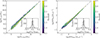 |
Fig. A.1. Comparison between the best-fit parameters derived from SED-fitting tests using mock SEDs and the corresponding input (ground truth) values. Data points are color-coded by redshift. The light gray error bars represent the uncertainties from the SED fitting process. The left panel shows results for stellar mass, while the right panel displays results for SFR. Insets in each panel present histograms of the logarithmic differences between the recovered and input values, with black dashed lines indicating the median offsets. |
Appendix B: The importance of F090W and F410M data
Although some medium-band filters, such as F410M, are available in our field, we excluded them from the primary analysis due to their relatively shallow depth. However, recent studies have highlighted the importance of medium-band data in accurately constraining galaxy physical properties, particularly at high redshifts where strong emission lines can significantly influence broadband photometry (e.g., Davis et al. 2024; Harvey et al. 2025). To evaluate the potential impact of including medium-band data, we conduct a test using the JADES-GDS dataset, focusing on the effect of incorporating the F410M filter into our SED fitting. We re-fit the physical properties of our selected high-quality sample after adding F410M data using the same methodology outlined in Section 3.1. The results are presented in Figure B.1, panels (a) and (b), in a format consistent with Figure A.1. The x-axes correspond to results obtained without the F410M band, while the y-axes show the results with F410M included.
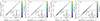 |
Fig. B.1. Similar to Figure A.1, but comparing the best-fit parameters derived from SED fitting using different filter configurations against those obtained with the full 10-filter set from the JADES-GDS field. Panels (a) and (b) show results with the F410M band included, while panels (c) and (d) show results with the F090W band excluded. |
As illustrated in the figure, the inclusion of F410M has a negligible effect on the derived physical parameters. It is worth noting that the F410M band was included in the photometric redshift measurement step, as medium-band data are known to significantly improve redshift accuracy (e.g., Davis et al. 2024). However, our results in Figure B.1 suggest that, once the redshift is fixed, the inclusion or exclusion of F410M has minimal impact on the estimation of galaxy physical properties.
In addition, we note that the CEERS field lacks imaging in the F090W band, unlike the other fields used in our analysis. Although CEERS data are not included in our primary results, we have confirmed that their inclusion does not substantially affect our conclusions. To specifically evaluate the impact of the missing F090W data on the estimation of galaxy physical properties, we conduct a controlled test using the JADES-GDS dataset, following the same methodology applied to assess the influence of F410M. We re-fit the physical properties of our selected high-quality sample when missing F090W data. The results are shown in panels (c) and (d) of Figure B.1. As demonstrated, the absence of F090W leads to a slight underestimation of stellar mass and a mild overestimation of the SFR. However, the median offsets are close to zero, and the scatter remains below 0.1 dex. These findings indicate that, even without F090W coverage, the derived physical properties remain robust and within acceptable uncertainties.
Appendix C: PSF smearing effect
In this work, we measure galaxy profiles directly from PSF-matched images with a radial step of 0.2Re. However, PSF smearing can wash out gradient information on scales comparable to the PSF (e.g., Liu et al. 2018; Hasheminia et al. 2024). Although, in Section 4.4, we have measured sSFR gradients using radial separations larger than the PSF FWHM to minimize the impact of PSF smearing on our results, some studies suggest that deconvolved images are more appropriate for mitigating PSF effects (e.g., Szomoru et al. 2013; Suess et al. 2019; Mosleh et al. 2020; Suess et al. 2022; Miller et al. 2023). Additionally, some studies also suggested that the radial steps should be larger than the PSF half-width at half-maximum to account for correlated noise (e.g., de la Vega et al. 2025). In this section, we also present the results obtained from the deconvolved images to test the roboustness of our results3.
Following the method described in the previous studies, we obtain the deconvolved images in every band of each galaxy by fitting the corresponding image with a single Sérsic model. Then a first-order correction is applied to the deconvolved models by adding the residual flux between the observed image and the PSF-convolved model. Based on the rest-frame 1 μm morphology, we construct a series of concentric elliptical annuli with a radial step of 2 pixels (0.08 arcsec), exceeding the PSF half-width at half-maximum. We then estimate the physical-property profiles following the procedure described in Section 3.4.
Using the same methodology as in Section 4, we also derive the median profiles of galaxies across different redshift and stellar-mass bins. The results are presented in Figure C.1. It can be seen from this figure, after accounting for PSF smearing, the results are largely consistent with those presented in Figures 9–11. As in Section 4.4, we also estimate the corresponding sSFR gradients, with the results presented in Table 1. For low-mass galaxies, the transition in sSFR gradients becomes even more pronounced. In contrast, for massive galaxies, the central sSFR shows mild suppression, and the transition in sSFR gradients between 0.5 kpc and 2.5 kpc is less evident. However, when a larger radial range is considered to derive the sSFR gradient, negative gradients can also be observed at high redshift.
All Tables
All Figures
|
Fig. 1. Redshift and stellar mass distribution of our total good sample. The region enclosed by the dashed black lines indicates the selected sample we used, defined by 0 < z < 4 and log(M*/M⊙) > 8. The solid cyan curve represents the 90% stellar mass completeness limit, which corresponds to a magnitude limit of F444Wlim = 28 mag. The gray (yellow) histograms in the top and right panels show the redshift and stellar mass distributions of the good sample (selected sample), respectively. |
| In the text | |
|
Fig. 2. Fraction of enclosed light as a function of radius for each filter relative to F444W in the JADES-GDS field. The upper and lower panels present the results before and after PSF matching, respectively. |
| In the text | |
|
Fig. 3. Example of our spatially resolved SED fitting for a randomly selected galaxy. The left panel shows the F444W-band image, and the dashed black lines mark elliptical annuli spaced at intervals of 0.2Re. Four representative radial regions are highlighted in red, orange, cyan, and magenta, corresponding to 0 < r < 0.2Re, 0.4Re < r < 0.6Re, 1Re < r < 1.2Re, and 2Re < r < 2.2Re, respectively. The middle and right columns display the SED fitting results for these four radial bins. |
| In the text | |
|
Fig. 4. Distribution of galaxy SFR as a function of stellar mass across different redshift bins. Each panel corresponds to a different redshift interval. The gray contours enclose 25%, 50%, 75%, and 99% of the galaxy population, respectively. The solid gray line in each panel indicates the sSFR threshold of 1/tH, where tH is the Hubble time at the median redshift of the bin; galaxies above this threshold are classified as SFGs. The black points with error bars represent the median SFR and the corresponding scatter for SFGs in different stellar mass bins. The solid black line shows the best-fit SFMS assuming the formulation in Equation (1), while the solid orange and red lines corresponds to the best-fit results derived from Equations (2) and (3), respectively. For comparison, we include results from previous studies: the dashed cyan line denotes the SFMS from Speagle et al. (2014), and the dashed orange and violet lines represent results from Popesso et al. (2023) and Koprowski et al. (2024), respectively. |
| In the text | |
|
Fig. 5. Left panel: Distribution of SFR for SFGs mapped onto the stellar mass vs. Universe age plane, where the color scale indicates the median SFR within each square bin. Middle panel: Best-fit SFMS derived using a linear relation. Right panel: Residuals between the observed SFRs and the best-fit linear model. The small residuals demonstrate that a linear relation provides a good representation of the SFMS for our sample across the explored stellar mass and cosmic time ranges. |
| In the text | |
|
Fig. 6. Distribution of galaxy sizes as a function of stellar mass for SFGs across different redshift bins. In each panel, the gray contours enclose 25%, 50%, 75%, and 99% of the sample. The black points with error bars denote the median effective radius and the corresponding standard deviation within stellar mass bins. The solid black line represents the best-fit size–mass relation derived from our analysis. For comparison, we show the results for the 0 < z < 0.5 bin as dashed gray lines in the remaining panels. |
| In the text | |
|
Fig. 7. Left panel: Distribution of size for SFGs mapped onto the stellar mass vs. redshift plane, where the color scale indicates the median size within each square bin. Middle panel: Best-fit models of the size mass relation. Right panel: Residuals between the observed size mass relation and the best-fit model. |
| In the text | |
|
Fig. 8. Two-dimensional histogram (blue) of the galaxy distribution with stellar mass ∼5 × 10¹⁰ M⊙. The orange contours enclose 25%, 50%, and 75% of the sample. The solid red line indicates the best-fitting relation derived in Section 4.2. To facilitate comparison with previous studies, the results from van der van der Wel et al. (2014), derived from rest-frame 0.5 μm sizes, are shown as black squares, and those from Martorano et al. (2024), derived from rest-frame 1.5 μm sizes, are shown as red stars. |
| In the text | |
|
Fig. 9. Radial profiles of stellar mass surface density for SFGs, categorized into three stellar mass intervals and eight redshift intervals. For each bin, we present the median Σ* as a function of radius, normalized by the Re (top row) and in physical units of kiloparsec (bottom row). To ensure the reliability of the profiles, we limit the radial range to regions where more than 50% of galaxies in the bin satisfy the adopted criterion for the signal-to-noise ratio. The shaded regions in the top panels denote the 25th–75th percentile distribution of Σ* at each radius. Due to the close of the profiles in physical units across different redshifts, we omit the corresponding distribution in the bottom panels for clarity. We also show the extent of the PSF FWHM using a shaded gray region in the bottom panel. For results in physical units, we also performed a linear extrapolation of the outer profiles, which is shown as a dashed line, to infer the stellar mass surface density in the galaxy outskirts. |
| In the text | |
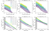 |
Fig. 10. Similar to Figure 9, but for radial profiles of ΣSFR. |
| In the text | |
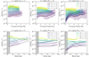 |
Fig. 11. Similar to Figure 9, but for radial profiles of sSFR. |
| In the text | |
|
Fig. A.1. Comparison between the best-fit parameters derived from SED-fitting tests using mock SEDs and the corresponding input (ground truth) values. Data points are color-coded by redshift. The light gray error bars represent the uncertainties from the SED fitting process. The left panel shows results for stellar mass, while the right panel displays results for SFR. Insets in each panel present histograms of the logarithmic differences between the recovered and input values, with black dashed lines indicating the median offsets. |
| In the text | |
|
Fig. B.1. Similar to Figure A.1, but comparing the best-fit parameters derived from SED fitting using different filter configurations against those obtained with the full 10-filter set from the JADES-GDS field. Panels (a) and (b) show results with the F410M band included, while panels (c) and (d) show results with the F090W band excluded. |
| In the text | |
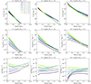 |
Fig. C.1. Similar to Figure 9 – 11, but for radial profiles derived from the deconvolved images. |
| In the text | |
Current usage metrics show cumulative count of Article Views (full-text article views including HTML views, PDF and ePub downloads, according to the available data) and Abstracts Views on Vision4Press platform.
Data correspond to usage on the plateform after 2015. The current usage metrics is available 48-96 hours after online publication and is updated daily on week days.
Initial download of the metrics may take a while.