| Issue |
A&A
Volume 708, April 2026
|
|
|---|---|---|
| Article Number | A347 | |
| Number of page(s) | 14 | |
| Section | Astrophysical processes | |
| DOI | https://doi.org/10.1051/0004-6361/202558687 | |
| Published online | 24 April 2026 | |
Unveiling the biconical geometry of the outflow in the ultraluminous X-ray source NGC 5204 X-1
1
Università degli Studi di Palermo, Dipartimento di Fisica e Chimica, Via Archirafi 36, I-90123 Palermo, Italy
2
INAF – IASF Palermo, Via U. La Malfa 153, I-90146 Palermo, Italy
3
Center for Astrophysics | Harvard & Smithsonian, 60 Garden Street, Cambridge, MA 02138, USA
4
Centre for Astrophysics Research, University of Hertfordshire, College Lane, Hatfield AL10 9AB, UK
5
School of Physics & Astronomy, University of Southampton, Southampton, Southampton SO17 1BJ, UK
6
Institute of Astronomy, University of Cambridge, Madingley Road, Cambridge CB3 0HA, UK
7
INAF – Osservatorio Astronomico di Brera, Via Brera 28, I-20121 Milano, Italy
★ Corresponding author: This email address is being protected from spambots. You need JavaScript enabled to view it.
Received:
19
December
2025
Accepted:
1
March
2026
Abstract
Context. Ultraluminous X-ray sources (ULXs) are non-nuclear X-ray binary systems that exceed the Eddington luminosity for a 10 M⊙ black hole. The majority of these sources are thought to be stellar-mass compact objects accreting at super-Eddington rates, exhibiting powerful relativistic winds. These winds have been identified through the detection of absorption lines with a blueshift as high as 0.3c and emission lines typically found at their laboratory wavelengths.
Aims. In this work, we analysed the XMM-Newton data of the ULX NGC 5204 X-1, which has been observed to exhibit emission lines with a blueshift of about 0.3c. The aim of this study is to examine the geometry and physical properties of the accretion disc and the relativistic outflows. In addition, we aim to explore the factors that influence the ULX spectral transitions.
Methods. We undertook an observing campaign with XMM-Newton to explore the source behaviour at different luminosities. In this first paper of the series, we performed high-resolution X-ray spectroscopy, including archival data, with the Reflection Grating Spectrometer (RGS) instrument, which allowed us to resolve both emission and absorption lines. The outflows features were characterised using physical models of plasma in collisional ionisation and photoionisation equilibrium.
Results. We identify collisionally ionised blueshifted and redshifted components at about 0.3c. These findings have a high statistical significance and suggest a biconical structure for the outflow. Additionally, the analysis of the O VII line triplet observed in the spectrum enables us to infer physical properties of the low-velocity line-emitting plasma; for example, electron density (ne ∼ 1010 cm−3) and temperature (Te ≥ 1.5 × 10⁵ K). A hybrid plasma whose ionisation balance is affected by both collisions and radiation is favoured.
Key words: accretion / accretion disks / X-rays: binaries / X-rays: individuals: NGC 5204 X-1
© The Authors 2026
 Open Access article, published by EDP Sciences, under the terms of the Creative Commons Attribution License (https://creativecommons.org/licenses/by/4.0), which permits unrestricted use, distribution, and reproduction in any medium, provided the original work is properly cited.
This article is published in open access under the Subscribe to Open model. This email address is being protected from spambots. You need JavaScript enabled to view it. to support open access publication.
1. Introduction
Ultraluminous X-ray sources (ULXs) are bright, mainly extragalactic, non-nuclear, point-like sources, emitting in the X-ray band with luminosities above 1039 erg/s, which corresponds to the Eddington limit for a 10 M⊙ black hole (BH), assuming a steady and spherical emission (for recent reviews, see King et al. 2023; Pinto & Walton 2023). The X-ray emission stems from the accretion of matter onto a compact object; however, the nature of ULXs has been highly debated, with two main possible scenarios. They can be powered by intermediate-mass black holes (IMBHs, 102 − 4 M⊙; Colbert & Mushotzky 1999), accreting at sub-Eddington rates, or by compact objects with smaller masses, such as neutron stars (NSs) and stellar-mass BHs, accreting at super-Eddington rates. This latter scenario is supported by the discovery of coherent pulsations in numerous sources (the first being M82 X-2, Bachetti et al. 2014), unambiguously confirming the accreting compact object to be a NS, and in turn revealing highly super-Eddington luminosities. Additionally, ULX spectra differ from those of the sub-Eddington Galactic BH X-ray binaries (XRBs): the former are characterised by a soft excess, usually modelled by a low-temperature blackbody component, plus a second thermal component with a curvature above 2 keV, which might originate from a supercritical accretion disc (Gladstone et al. 2009; Bachetti et al. 2013). Additionally, evidence has emerged of a third, harder continuum component, revealed by high-statistics NuSTAR data (Walton et al. 2018). Its origin is thought to be related to photon scattering, either in an optically thin corona or within the accretion column onto a magnetised NS (Brightman et al. 2016; Walton et al. 2018).
The theory of super-Eddington accretion predicts an accretion disc around the compact object that is geometrically and optically thick inside the spherisation radius, and within this radius an optically thick outflow, with a clumpy nature, is launched from the top of the disc by the radiation pressure (e.g. Ohsuga et al. 2005; Poutanen et al. 2007; Takeuchi et al. 2013). Due to the resulting funnel shape of the accretion disc and wind combination, the spectral hardness of the source below 10 keV – typically defined for XMM-Newton data as the ratio between the flux in the 2 − 10 keV and in the 0.3 − 2 keV energy bands – depends on the viewing angle (e.g. Middleton et al. 2015a): at low inclinations from the rotational axis, the spectrum will appear hard (hard-ultraluminous regime or HUL), as we are able to see the innermost and hotter regions of the accretion disc; at higher angles, the hard X-ray emission is obscured by the disc and outflow, resulting in a softer spectrum (soft-ultraluminous regime or SUL, e.g. Sutton et al. 2013).
Several spectral features are observed in the soft energy band, below 2 keV, which have been identified thanks to the high-resolution grating spectrometers on board XMM-Newton and Chandra (e.g. Pinto et al. 2016, 2017; van den Eijnden et al. 2019). Evidence of corresponding features has also been found in CCD data, in most cases with high-count spectra (see e.g. Stobbart et al. 2006; Middleton et al. 2015b) and in a few cases even in the Fe K band (6 − 9 keV, e.g. Walton et al. 2016; Brightman et al. 2022). Their detection is important, as they reveal information on the geometry of the accretion disc and on the presence of outflows driven by the radiation pressure, which supports the scenario of super-Eddington accretion. Mildly relativistic outflows have been detected in many sources (see the first catalogue of spectral lines in a sample of ULXs by Kosec et al. 2021).
2. NGC 5204 X-1
NGC 5204 X-1 is a bright and persistent ULX located at a distance of 4.5 Mpc (Bottinelli et al. 1984), with an observed (average) X-ray luminosity LX ∼ 4.5 × 1039 erg/s (Mukherjee et al. 2015) in the 0.3 − 10 keV energy range. The source mostly switches between intermediate-HUL, bright-SUL, and faint-supersoft (SSUL) X-ray regimes. Furthermore, it shows a putative quasi-periodic flux modulation over a timescale of about 200 days (Gúrpide et al. 2021b), likely due to a variation in the mass accretion rate or the system geometry. NGC 5204 X-1 shows evidence of an ultrafast outflow (UFO) with a velocity of about −0.3c, revealed by the detection of blueshifted emission lines, making it the fastest outflow ever recorded in a ULX. Specifically, it is the only ULX in which a UFO has been detected in emission; in other ULXs, such as NGC 1313 X-1 (Pinto et al. 2020) and the pulsating NGC 300 ULX-1 (Kosec et al. 2018b), UFOs have instead been detected in absorption. This highly blueshifted emitter was modelled assuming the plasma in collisional ionisation equilibrium (CIE) by Kosec et al. (2018a) with a cumulative significance of 3σ. They also find similarities with the source SS433, the only known persistent super-Eddington accretor in our Galaxy, in which relativistic blue- and redshifted emission lines from collisionally ionised jets have been detected (Marshall et al. 2002).
The primary goals of this work are (i) to investigate the spectral transitions observed in ULXs, which might be driven by the wind, the accretion rate, or the precession of the inner accretion flow and (ii) to constrain the structure of the outflow in analogy with the Galactic source SS433. To this aim, we used XMM-Newton data, combining archival data with two newly acquired long-exposure observations. The paper is organised as follows: in Section 3, we describe the available observations and the data reduction procedure; Section 4 presents the spectral continuum modelling and the different methods used to investigate the outflows; in Sections 5 and 6, we discuss and summarise our results.
3. Observations and data reduction
We used data from all available XMM-Newton observations of NGC 5204 X-1 between 2003 and 2023 (see Table 1), including the last 240 ks campaign (ObsIDs 0921360101 and 0921360201; PI: Pinto). The analysis is based on data from the European Photon Imaging Camera (EPIC) and the Reflection Grating Spectrometer (RGS) on board XMM-Newton. The EPIC cameras are useful to provide an accurate description of the spectral continuum, while RGS is used to detect narrow spectral features in the soft X-ray band. The latter campaign was split into two epochs separated by 6 months during 2023, in order to investigate the source in two different flux regimes. Through a Swift X-ray Telescope (XRT; Gehrels et al. 2004) monitoring, we triggered two observations. The first was obtained when the source was in the unobscured bright-SUL regime (ObsID 0921360201), specifically when the source XRT count rate was above 0.07 counts/s and the hardness (calculated as the ratio between the counts in 1.5 − 10 keV and 0.3 − 10 keV bands) was below 0.4. The second observation was triggered when the source was in the intermediate-HUL regime (ObsID 0921360101), when the count rate was between 0.05 − 0.07 counts/s and the hardness above 0.4. These flux regimes are representative of previously observed states of the source, as XMM-Newton has observed NGC 5204 X-1 in both the bright-SUL regime (EPIC-pn count rates > 0.7) and the intermediate-HUL regime (EPIC-pn count rates ∼0.5; see Table 1).
Table of the XMM-Newton observations of NGC 5204 X-1.
In order to visualise the spectral variability of the source, we extracted the XRT light curve of NGC 5204 X-1 in the 0.3 − 10 keV energy band, using the website tool1 (Evans et al. 2009). The XRT monitoring was performed from April 2013 to February 2025. As the XMM-Newton spectra from all observations show flux variability below approximately 3 keV (see also Gúrpide et al. 2021a), we computed the spectral hardness of the XRT data as the ratio between the flux in the 3 − 10 keV and in the 0.3 − 3 keV energy bands. Figure 1 shows the XRT light curve and hardness ratio, with the dashed lines marking the start times of the two most recent deep XMM-Newton observations, as well as the histogram of the count rates derived from the light curve.
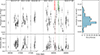 |
Fig. 1. Left: Swift/XRT light curve (top) and hardness ratio curve (bottom) of NGC 5204 X-1 from April 2013 to February 2025. The hardness ratio is defined as the ratio between the XRT counts in 3 − 10 keV range and those in 0.3 − 3 keV. The dashed red and green lines indicate the start times of the two latest XMM-Newton observations. Right: Corresponding count rate histogram. |
The observational data files (ODF) were downloaded from the XMM-Newton Science Archive (XSA)2 and we performed the standard data reduction procedure using the Science Analysis System (SAS) version 21.0.03 with recent calibration files (April 2024). The cleaned event files of the EPIC-pn and MOS 1,2 cameras were created through the epproc and emproc tasks, respectively. Periods of high background rate (e.g. due to solar flares) were excluded using the evselect task by considering the light curves above 10 keV, with thresholds of 0.5 counts/s for pn and 0.35 counts/s for MOS 1,2. In addition, we filtered the data to account for bad pixels and bad columns. Events with PATTERN< = 4 (single and double) were accepted for pn data, while for MOS 1, 2 data, events with PATTERN< = 12 (up to quadruple) were considered.
To extract spectra, we chose a circular region for the source of 20 arcsecond radius centred at the source position (Chandra co-ordinates: RA = 13h 29m 39s, Dec = +58° 25′ 06″). For the background, a circular region of 50 arcsecond radius was selected away from the source on the same chip, in order to avoid the contamination from the copper ring and the chip gaps. To produce response matrices and effective area files, we used the rmfgen and arfgen tasks. We also produced stacked spectra for each EPIC camera using epicspeccombine to deepen our search for features in the full time-averaged spectra obtained by combining all observations, and in the archival data (hereafter archive-only), to validate the result of Kosec et al. (2018a) and corroborate our new method.
The event files of RGS 1,2 were created using the rgsproc task, which also produces spectra and response matrices. Periods of high background rate were filtered out by examining the background light curve from RGS 1,2 CCD number 9 and rejecting time bins with a count rate exceeding 0.2 counts/s. Subsequently, we extracted the first-order spectra by considering 90% of the source point spread function, and the background spectra by selecting photons beyond 98% of the point spread function. The individual RGS 1 and 2 spectra from observations 0921360101 and 0921360201 contain about 2200 net source counts each. As the individual first-order RGS 1 and 2 spectra of each observation were superimposable in the band of interest (0.45 − 1.77 keV), we stacked them using rgscombine to decrease the number of spectra to be analysed and speed up the computational time, which is necessary for Monte Carlo simulations aimed at estimating the significance of line detection (see Sect. 4.4).
As was previously done for EPIC cameras, we also stacked the RGS spectra for the archive-only data obtaining a spectrum fully compatible with that of Kosec et al. (2018a) and a very deep time-averaged spectrum corresponding to a total exposure of about 420 ks and roughly 11 000 net source counts. We also extracted the second-order RGS 1 and 2 spectra, but since they are highly affected by the instrumental background, we did not use them in the analysis.
4. Spectral analysis
In this section, we present the spectral analysis of NGC 5204 X-1. We first focused on modelling the spectral continuum. Next, we performed a Gaussian line scan to search for and identify any spectral features. Finally, we tested different physical plasma models to study the nature of the spectral features and the structure of the outflows responsible for them. The spectral analysis was performed using SPEX version 3.07.03 (Kaastra et al. 1996, 2022). The spectra were grouped according to the optimal binning criterion as defined in Kaastra & Bleeker (2016) using the obin command in SPEX, and were fitted by minimising the Cash statistics (C-stat; Cash 1979). The errors in the model parameters correspond to 1σ confidence level. We adopted solar abundances from Lodders et al. (2009), which are default in SPEX. The spectral ranges used for our spectral analysis are: 0.3 − 0.5 keV and 1.77 − 10 keV for EPIC, and 0.45 − 1.77 keV (i.e. 7 − 27 Å) for RGS because for lower energies the background dominates the source spectrum. We ignored the EPIC data in the 0.5 − 1.77 keV range to employ the high spectral resolution of RGS and reduce the degeneracy between emission and absorption line models, while still maintaining a good handle on the continuum through the EPIC data (e.g. Pinto et al. 2021). When including EPIC data in the 0.5 − 1.77 keV range, the continuum parameters vary at the 10 − 20% level, consistent with continuum uncertainties. We notice that in this work we do not perform a dedicated broadband, time-resolved study, in particular, of the evolution of the continuum properties which will be the focus of a companion paper (Barra et al., in prep.).
4.1. Continuum modelling
We simultaneously fitted the EPIC-pn, MOS 1,2, and RGS full time-averaged spectra. To account for cross-instrument calibration uncertainties, which we found to be between 2% and 10%, we included a free multiplicative constant in the model, fixing it to unity for EPIC-pn. The spectral continuum is modelled as hot*(bb+comt), comprising two emission components. The bb component represents the blackbody emission from the outer parts of the accretion disc or the wind, while the comt component describes the Comptonisation of soft photons in a hot plasma. This process might originate from the scattering of photons emitted within the geometrically thick disc (see e.g. Middleton et al. 2015a). Additionally, we coupled the temperature of the bb component to the temperature of the seed photons of the comt component. The absorption by the foreground interstellar and circumstellar media was accounted for using the hot component, and we fixed the temperature at 10−6 keV, to describe a neutral gas. We also tested other continuum models such as hot*(dbb+comt), where dbb describes the emission of a multi-temperature disc blackbody, but the fit remained approximately unchanged. The best-fit hydrogen column density, NH, is  cm−2, about twice the Galactic value estimated by Dickey & Lockman (1990), and implies additional absorption in the NGC 5204 galaxy. The time-averaged spectra, along with the best-fit continuum model and residuals, are shown in Fig. 2. It is possible to observe some residuals around 0.6 keV and 1 keV, which hint at the presence of spectral lines.
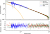 |
Fig. 2. EPIC-pn (black), MOS 1 (red), MOS 2 (green), and RGS (blue) spectra and the best-fit continuum model (red curve), from the stacking of all XMM-Newton observations. The continuum emission components are represented by dashed lines in orange (bb) and green (comt). The EPIC data are ignored in the 0.5 − 1.77 keV energy range to employ the full high spectral resolution of RGS and avoid model degeneracy. The EPIC data are grouped according to the optimal binning and, for a better visualisation, the RGS data are grouped by a factor of 9. The bottom panel shows the residuals of the best-fit model. |
A spectral fitting for the characterisation of the continuum is also performed for the combined archive-only data and for the two most recent observations, to reproduce the results already obtained by Kosec et al. (2018a) and to study the variability of the spectra between observations in two different flux regimes. In this and all subsequent analyses, the value of NH was fixed to that derived from the fit of the time-averaged data, as the amount of plasma in the interstellar medium is not expected to vary significantly across observations. The best-fit results for the different datasets are shown in Table 2.
Results of the best-fit continuum modelling.
4.2. Gaussian line scan
In order to search for spectral lines due to the presence of outflows, we first performed a scan of the spectra with a moving Gaussian line. We added a Gaussian line to the best-fit continuum model using the gaus component in SPEX with a specific centroid energy and line width. The model was fitted for the normalisation of the line allowing for both positive and negative values, corresponding to emission and absorption lines, respectively, along with the continuum. The C-stat was saved and compared to the value obtained by the fit of the continuum-only model, computing the ΔC-stat improvement. We then varied the centroid energy of the line over a logarithmic grid ranging from 0.5 to 8 keV, searching for spectral lines also outside the RGS energy range – where the EPIC source spectra lie well above the background. The number of grid points ranged from 500 to 4000, as we varied the velocity dispersion, σv, from 2500 to 100 km/s. The single-trial significance of each line was calculated as the square root of the ΔC-stat improvement times the sign of the normalisation of the line to distinguish between absorption and emission features. Nevertheless, this method does not take into account the look-elsewhere effect, such as spurious features associated with Poisson noise, resulting in an overestimate of the significance of individual lines (Protassov et al. 2002). The real significance of the spectral features can be estimated by running Monte Carlo simulations (see Section 4.4). The results of the line scan are shown in Figure 3.
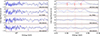 |
Fig. 3. Gaussian line scan performed on the four analysed datasets. We show the results for velocity widths of 2500 km/s (solid grey line) and 100 km/s (dotted blue line). The 3σ threshold (red line) is shown. In the right panel, a zoom in the 0.5 − 0.6 keV energy range is shown to better visualise the O VII line triplet, with the red lines showing the positions of the rest-frame energies. |
We first performed the line search in the combined archive-only data. There are strong emission features with a ΔC-stat ∼12 at 1.2 keV (∼10 Å) and at about 0.57 keV (∼22 Å), analogously to what is found in Kosec et al. (2018a). Then, we performed the line search on the full time-averaged spectra and on the individual observations. At about 2.2 keV, for the time-averaged spectra and for the observation 0921360201, we see an absorption feature, due to an absorption edge characteristic of the instrument, likely corresponding to the Au-M edge. For the time-averaged spectra, we find strong emission features at about 0.8 keV (∼15 Å) with a ΔC-stat ∼14 and at about 0.57 keV (∼22 Å) with a ΔC-stat ∼12. There is evidence of an absorption feature at 0.6 keV (∼20 Å), also found in the observation 0921360101 (ΔC-stat ∼17). In the observation 0921360201, there is evidence of an absorption feature at about 0.7 keV (ΔC-stat ∼14). Specifically, the emission lines found in common between the archive-only and time-averaged data at about ∼22 Å correspond to the O VII triplet, with the resonance line (r) at 21.6 Å, intercombination line (i) at 21.8 Å, and forbidden line (f) at 22.1 Å (see Figure 3). The resonance line seems to be blueshifted, hinting at an outflow moving towards us. We modelled the O VII triplet in the time-averaged data with simple Gaussian profiles to obtain some information about the physical state of the plasma by calculating the G-R line ratios, as illustrated in Section 5.1. There is no significant evidence of the O VII triplet or other strong emission lines in the two most recent observations.
4.3. Physical model scans
In order to identify the nature of the spectral features, we employed physical models of line emission or absorption, performing spectral scans in a multidimensional parameter space for a plasma in CIE and photoionisation equilibrium (PIE). This approach allows us to simultaneously fit multiple lines reducing the risk of getting stuck in local minima and allowing for the identification of multiple phases of the plasma. We searched through the parameter space of the line-of-sight velocity, vLOS, and the key plasma property (the temperature, kT, for CIE or the ionisation parameter, ξ, for PIE). This method essentially builds on the previous works of Kosec et al. (2018b) and Pinto et al. (2020).
4.3.1. Collisionally ionised plasma in emission
In the case of a line-emitting CIE plasma, we adopted the cie model in SPEX, which calculates the emitting spectrum for a plasma in CIE. Additionally, to account for possible blueshifted and/or redshifted emission lines, we added the reds component that multiplies the cie model, with FLAG = 1 to apply a Doppler shift rather than a cosmological redshift. We constructed a grid of plasma temperatures, kT, line-of-sight velocities, vLOS, and velocity dispersions, σv. We adopted a logarithmic grid of temperatures spanning the range 0.1 − 6 keV, sampled at 20 points, and a linear grid of line-of-sight velocities from −0.4c (blueshifted outflow) to +0.4c (redshifted outflow). The velocity dispersion was decreased from 2500 to 100 km/s, with steps from 1000 to 500 km/s for the line-of-sight velocity. The normalisation of the cie component corresponding to the emission measure, nHneV – with ne and nH denoting the electron and hydrogen densities, respectively, and V the volume of the line-emitting plasma – was left free to vary. For each combination of (kT, vLOS, σv), we recorded the ΔC-stat improvement with respect to the continuum-only model. In Fig. 4, we show the results of the scan for the four different datasets. The CIE solutions are found mainly at kT ≲ 1.5 keV, which means that the results are driven primarily by the RGS data.
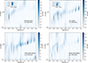 |
Fig. 4. CIE model scan performed on the four analysed datasets, adopting a velocity dispersion of 250 km/s. The colours show indication of the ΔC-stat improvement compared to the continuum-only model. The black contours refer to significance levels from 2.5 to 3.5σ with steps of 0.5σ estimated with Monte Carlo simulations (see Section 4.4). |
Our analysis of the combined archive-only data finds a fit improvement with respect to the continuum model, with a ΔC-stat = 24 for a velocity dispersion of 250 km/s, a cie temperature of approximately 0.45 keV, and a line-of-sight velocity of −0.3c (see Table 3). Kosec et al. (2018a) find a solution that corresponds to a secondary peak in our maps at −0.33c. Additionally, we also find an independent solution with a ΔC-stat = 16 that describes a lower-temperature plasma (kT∼0.1 keV) close to rest-frame. This component is primarily responsible for the O VII line emission. For other values of the velocity dispersion, we do not obtain larger fit improvements.
Best-fit parameters of the cie models applied on the continuum model for the four analysed datasets.
From the analysis of the time-averaged spectra, we find two line-emitting components: one with a temperature of about 0.4 keV and outflow velocity of approximately −0.30c (ΔC-stat = 24, see Table 3), another component with a temperature of 1.65 keV and an outflow velocity of about 0.35c (ΔC-stat = 30). Another solution is found at a temperature of approximately 0.2 keV that describes an approximately rest-frame plasma (ΔC-stat = 18). Additional solutions appear at velocities of about −0.2c with temperatures comparable to those of the components discussed above – potentially reproducing similar spectral features – but with lower ΔC-stat values. The technical evaluation of secondary solutions is performed in Appendix A. For observations 0921360101 and 0921360201, the fit improvement is lower (ΔC-stat = 15 − 17). For each dataset, we then fitted the EPIC and RGS spectra adding to the continuum the cie models with higher ΔC-stat values, in order to better describe the spectra and identify the contribution of each cie to the observed emission lines (see Section 4.5).
4.3.2. Photoionised plasma
A plasma in PIE is described by the ionisation parameter, ξ = Lion/nHR2, where Lion is the luminosity of the ionising source, nH is the hydrogen number density, and R is the distance of the plasma from the source. The ionisation balance depends on the relative elements abundance; in this work, we adopted solar abundances as for the interstellar medium absorber. We computed the ionisation balance using the pion code (Mehdipour et al. 2016; Miller et al. 2015), which performs an instantaneous calculation of the balance, adopting the best-fit continuum model (see Table 2) as the spectral energy distribution (SED). Another way of computing the ionisation balance consists of the use of the xabsinput tool in SPEX, which produces tables of the temperature and ionic column density as functions of the ionisation parameter, ξ. These outputs are used by the xabs model to compute the spectrum of a photoionised plasma in absorption. We obtain similar results with both methods.
The ionisation balance depends on the relationship between the ionisation parameter and the temperature, which is illustrated in Figure 5. An alternative way of illustrating the ionisation balance is through the stability curve, also known as the S curve, which shows the temperature as a function of the ratio between the radiation pressure (L/4πR2c) and the thermal pressure (nHkT), which is given by Ξ = 19222 ξ/T. Along this curve, heating equals cooling, which means that the gas is in thermal balance (Krolik et al. 1981). The photoionised plasma is thermally stable for Ξ values corresponding to positive slopes of the S curve, while negative slopes indicate thermal instability to temperature perturbations. The presence of unstable branches may produce a multiphase plasma. We would not typically expect to find (T,Ξ) solutions occupying unstable branches unless short-lived events occur.
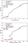 |
Fig. 5. Ionisation balance (top) and stability curve (bottom) for the time-averaged spectra, archive-only data, and new individual observations, using as the SED the best-fit continuum model for each case. Thick blue and red segments show the ranges of the best-fit solutions from the pion and xabs models. |
In the case of the emitting plasma in PIE, we adopted the pion component, which was included additively in our spectral model, on top of the continuum, and a reds component was applied to account for Doppler shifts. Additionally, we adopted for pion a full solid angle of Ω = 4π, representing the emission from a thin shell, and a covering fraction, fcov, of zero, to produce only emission lines. We performed a spectral scan using the pion model creating a grid of (vLOS, ξ, σv). Specifically, we varied log ξ from 0 to 6 with 0.1 steps, and scanned vLOS from −0.4c to +0.4c to reproduce both blueshifted and redshifted emission lines. We tested different velocity dispersions (σv= 100, 250, 500, 1000, 2500 km/s). The column density, NH, of the pion component was left free to vary. The results of the scans for the four datasets are shown in Fig. B.1.
Specifically, from the analysis of the time-averaged spectra, we obtain a fit improvement of ΔC-stat = 24 for a blueshift of about 3900 km/s and an ionisation parameter of log ξ ∼ 0.2 (corresponding to a T ∼1.5 × 10⁴ K), assuming a velocity dispersion of σv = 250 km/s. A smaller improvement (ΔC-stat = 17) but with similar values of vLOS and log ξ is obtained from the scan of the archive-only data. Additionally, the scan of the time-averaged spectra reveals another improvement (ΔC-stat = 20) for vLOS ∼ −0.2c and log ξ ∼ 2.7 (corresponding to a T ∼6 × 10⁵ K), under the same assumption of σv = 250 km/s. Similarly, the archive-only data shows a fit improvement of ΔC-stat = 21 for a vLOS ∼ −0.05c and log ξ ∼ 0.1. The scan of individual observations shows similar but less significant results, with no remarkable improvements in observation 0921360201.
In the case of the absorbing plasma in PIE, we computed the ionisation balance through the xabsinput tool in SPEX. We then performed a spectral scan using the faster xabs model exploring the ξ − vLOS parameter space. The value of log ξ was varied from 0 to 6 with 0.1 steps, and vLOS from −0.4c to 0, to reproduce only blueshifted absorption lines due to outflows. We tested different velocity dispersions (σv = 100, 250, 500, 1000, 2500 km/s). For each combination of (log ξ, vLOS, σv), we fitted the column density, NH, of the xabs component. In Fig. B.2, we show the results of the scans for the different datasets.
For ObsID 0921360101, higher values of ΔC−stat are found; specifically, we obtain a fit improvement of ΔC-stat = 23 for a vLOS ∼ −0.05c and log ξ ∼ 1, adopting σv = 2500 km/s. The same is observed for the archive-only and time-averaged data, but with a much lower ΔC-stat (< 13). For ObsID 0921360201, we obtain a fit improvement of ΔC-stat = 17 for a vLOS ∼ −0.09c and log ξ ∼ 4.2, adopting σv = 1000 km/s.
4.4. Significance estimates through Monte Carlo simulations
The significance of the detection of a line-emitting or line-absorbing plasma through the use of physical model grids is obtained by performing identical multi-parameter searches for a large number of spectra simulated with SPEX, which only contain Poisson noise (and no outflow features), and are based on the best-fit continuum model. This enables us to account for the look-elsewhere effect. We used the method outlined by Pinto et al. (2020). In the case of NGC 5204 X-1, we simulated 5,400 EPIC and RGS spectra, adopting as a template the best-fit continuum model of the EPIC+RGS observation with ObsID 0921360101, and with the same exposure times of the real data. Each simulated spectrum was scanned with the cie model, using the same parameter space explored for the real data (Section 4.3.1). The histogram of the ΔC-stat values was produced to estimate the significance for the detection in the real data. This is shown in Figure 6. We adopted a velocity dispersion of σv = 1000 km/s, which is midway between the best-fit results of the individual components (see Table 3). The parameter space for this velocity dispersion is slightly smaller than that for narrower values (e.g. 250 km/s, for which a velocity step of 500 km/s was used instead of 700 km/s). However, this difference is not significant, as it remains well within the RGS spectral resolution. Indeed, a set of a thousand simulations performed with the narrower step yields a negligible change in the significance (∼0.1σ), which is within the uncertainty of the histogram slope (see Figure 6).
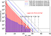 |
Fig. 6. Histogram of ΔC-stat values of a CIE model scan of the time-averaged data adopting a velocity dispersion of 250 km/s (blue bars), and of CIE model scans of 5400 Monte Carlo simulated data (red bars). Forecasts for more simulations are made assuming a constant slope of the histogram, in order to visualise different confidence levels. |
Since the histogram slope (∼ − 0.252) is approximately constant after a few thousand simulations, it is possible to forecast the results for a larger number of simulations re-scaling the normalisation of the best-fit power law (see Pinto et al. 2021; Gu et al. 2022). The false-alarm probability is estimated computing the fraction of simulations with the same or higher ΔC-stat than the value obtained for the real data. According to the simulations, ΔC-stat > 22 (29) would correspond to a confidence level above 3σ (4σ). The high significance of the observed spectral features allows us to make a comparison between the data and complex models, avoiding the risk of over-interpreting the data. We repeated the same procedure for the time-averaged data for a thousand simulations, and the histogram of the ΔC-stat values has a comparable slope.
4.5. Final fits with physical models
In order to investigate the nature of the plasma responsible for the observed emission and absorption lines, we performed spectral fits for the archive-only, full time-averaged, and the two most recent individual spectra, considering the results obtained by the physical model scans. Analogously to the analysis performed in Kosec et al. (2018a), we analysed the combined archive-only data by adding a blueshifted cie model on top of the continuum. The improvement of the fit yields a ΔC-stat = 26 for four degrees of freedom (nHneV, kT, σv, vLOS), adopting a volume density of 1010cm−3, estimated from the analysis of the O VII triplet (see Section 5.1). In particular, we assume that the volume density of the relativistic outflow is identical to that of the slow-moving plasma, as the available emission lines do not allow us to constrain or distinguish the densities of the two plasma components. The cie component exhibits a blueshift of ( − 0.2960 ± 0.0006)c and a temperature of  keV. We obtain a 1σ upper limit on the velocity broadening of 500 km/s. The emission features of the cie component are reproduced by Fe XVII and O VIII. Additionally, a further fit improvement (ΔC-stat = 15 respect with the previous model) is achieved with the addition of a rest-frame cie component, along with the blueshifted one. The plasma temperature of the rest-frame component is 0.12 ± 0.02 keV and the velocity dispersion is
  km/s. This second cie component reproduces the O VII emission, with a dominant resonance line as expected for a hybrid plasma where collisions are not negligible. The centroid of the resonance line seems to be blueshifted, while the intercombination and forbidden lines appear to be at rest.
For the time-averaged spectra, based on the results of the physical model scans, we added two cie components to the continuum model. A blueshift was applied to the first and a redshift to the second, and the velocity dispersion was linked between the two components. A total improvement of ΔC-stat = 57 compared to the continuum-only model is achieved (ΔC-stat = 25 and 32 for the individual blueshifted and redshifted cie components, respectively), confirming that the two solutions are independent and account for distinct spectral features. The first cie component exhibits a blueshift of  and a temperature of
  keV, consistent with the results from the archive-only data, while the second cie component shows a redshift of
  and a temperature of
  keV, with an 1σ upper limit on the velocity broadening of 200 km/s. The blueshifted cie model fits several emission lines, reproduced by Ne X, Fe XVII, and O VIII. Specifically, the dominant lines are the resonance (λ = 15 Å) and forbidden (λ = 17.1 Å) lines of Fe XVII, observed at ∼10 Å and ∼11.3 Å, respectively. The redshifted component fits other emission features, reproduced by Ne X, Fe XXIII, Fe XXIV, and O VIII. None of these fast components is able to reproduce the O VII line triplet, which is close to the laboratory wavelengths and was already observed in the archive-only data. Consequently, we tested the addition of a rest-frame cie component (ΔC-stat = 18) and a weakly blueshifted pion component (ΔC-stat = 22). The pion component exhibits a blueshift of
  km/s and a value of
  . We also fitted the volume density, obtaining a value of
  cm−3, consistent with the results from the analysis of the O VII triplet (see Section 5.1). This model reproduces the O VII emission, where the forbidden line is stronger than the other lines, as expected from a photoionised plasma. Figures 7 and B.3 show the best-fit models with the rest-frame cie and pion components, respectively. Similar analyses were performed for the two recent individual observations, with all best-fit results reported in Table 3 and Figure 8.
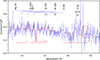 |
Fig. 7. RGS spectrum in the 7 − 27 Å range, obtained by stacking all XMM-Newton observations. The red curve shows the model with three cie components (blueshifted, redshifted, and rest-frame), on top of the continuum. The rest-frame wavelengths of the most relevant lines are labelled. The dotted (dashed) lines show the velocity shift for the blueshifted (redshifted) lines. The data are grouped by a factor of 10. |
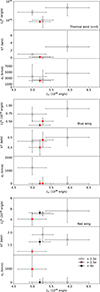 |
Fig. 8. X-ray (0.3 − 10 keV) luminosity, temperature, and velocity dispersion of the cie plasma components as functions of the continuum X-ray luminosity. Filled (empty) red dots show solutions with significance above (below) 2.5σ, and filled black dots are those above 4σ. |
Furthermore, as is suggested by the scan of PIE plasma in absorption for observation 0921360101, the addition of a xabs component improves the fit, obtaining log ξ = 1.00 ± 0.12, vLOS = ( − 0.051 ± 0.004)c, a ΔC-stat of about 23 for a velocity dispersion of  km/s. Using this model, the absorption feature we observed at 0.6 keV would be attributed to O VII.
5. Discussion
5.1. Physical properties of the line-emitting plasma
As first diagnostics of the plasma properties, we constrain the electronic density and temperature through the calculation of the R and G ratios for the He-like triplets, which are defined as follows (Porquet & Dubau 2000): R(ne) = f/i and G(Te) = (f + i)/r, where r, i, and f are the fluxes of the resonance, intercombination, and forbidden lines, respectively. We computed the R and G ratios for the O VII triplet, for which we found evidence in the Gaussian line scan (see Figure 3), by modelling the emission lines as simple Gaussian lines in the time-averaged spectra. As shown in Figure 3, a single set of three Gaussian lines does not provide a satisfactory fit, due to clear evidence of a blueshifted O VII resonance line. We therefore added two sets of three O VII lines to the best-fit continuum model: one at rest-frame energies, and a second set with a common blueshift applied, with all line energies fixed to their laboratory values. Additionally, their FWHMs were coupled. We fitted the line normalisations along with the continuum (see Figure 9). The best-fit yields a ΔC-stat = 26 compared to the continuum-only model. For the rest-frame O VII triplet, we obtain R = 0.4 ± 0.3 and a lower limit of G > 8, the latter resulting from the upper-limit on the normalisation of the resonance line. For the blueshifted emission lines, we find R ∼ 1.56, with only upper limits on the normalisations of the intercombination and forbidden lines, and an upper limit of G < 0.44. The blueshifted set of O VII lines have a common line-of-sight velocity of about 1500 ± 300 km/s.
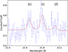 |
Fig. 9. Zoom on the O VII emission triplet (r: resonance, i: intercombination, f: forbidden; see Section 5.1) as fitted with two sets of three Gaussian lines (red) in the RGS time-averaged spectrum (blue). |
We computed the R and G ratios for the O VII triplet as functions of the electronic density, ne, and the electronic temperature, Te, respectively, using the SPEX pion code. The best-fit continuum model of the time-averaged spectra was used as the SED; the photoionisation balance was obtained with the ascdump command, along with the fluxes of the O VII lines. The computation was realised by varying log ξ between 0 and 4.0 with 0.2 steps, and ne from 108 to 1014 cm−3 with a logarithmic step of 10. We also adopted a velocity dispersion of 250 km/s, as it provides the best-fit improvement. The G and R ratios curves are shown in Fig. 10. Using the values of R and G obtained by the fitting of the rest-frame O VII emission lines, we obtain a number density around 3 × 1011 cm−3, with an upper limit of 1012 cm−3, and Te ≤ 1.5 × 10⁴ K, indicative of a PIE plasma. Based on the values of R and G from the blueshifted emission lines, we infer a number density around 4 × 1010 cm−3 and a temperature Te ≥ 1.5 × 10⁵ K, suggesting both a heating process and a CIE plasma. The values found for ne are consistent with those found for the ULX NGC 1313 X-1 (Pinto et al. 2020).
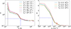 |
Fig. 10. G (left) and R (right) ratios curves for the O VII triplet. Blue arrows show upper and lower limits, corresponding to lower and upper limits on the temperature, respectively. The dashed black lines indicates the results obtained for the rest-frame O VII triplet, while the dashed blue lines for the blueshifted emission lines. In the right panel, the red point indicates the value of R obtained from the rest-frame O VII lines. |
5.2. Outflow structure and constraints on the ULX nature
The spectral scan of the time-averaged spectra with a CIE plasma model revealed evidence of two plasma components moving in the opposite directions along the line of sight, both with velocities of about 0.3c. Consequently, the two most recent deep observations helped us to investigate the structure of the outflow, revealing its biconical geometry. The archive-only data analysed in Kosec et al. (2018a) only allowed the detection of the collisionally ionised plasma blueshifted to about 0.3c. However, the individual observations do not provide sufficient statistics to identify significative variations in the outflow properties. As is shown in Figure 8, the outflow parameters are consistent across the different datasets, indicating the presence and stability of the outflow, as also supported by the higher significance obtained from the full time-averaged data.
Specifically, for the component outflowing at approximately −0.3c, we obtain a ΔC-stat = 25, resulting in a significance > 3σ, while for the component moving at about 0.3c, the ΔC-stat is 32, corresponding to > 4σ. The significances were estimated through Monte Carlo simulations. The luminosity of the first component is 4 × 1037 erg/s, while that of the second component is an order of magnitude higher (5 × 1038 erg/s). This is attributed to the blueshifted plasma being found to be cooler than the redshifted counterpart, possibly due to interactions with regions of the interstellar medium having different physical properties. Nevertheless, both the luminosities and the corresponding temperatures are consistent within a few sigma (see Figure 4).
Our results are similar to those reported for the Galactic source SS433, as previously noted in Kosec et al. (2018a), where the emission originates from oppositely directed plasma jets in CIE. The jets are accelerated to 0.27c and, accounting for projection effects, the blue jet is blueshifted by 0.08c and the red jet is redshifted by 0.16c (Marshall et al. 2002). Some lines are in common to our time-averaged spectra and the spectra of SS433, such as the Ne X Lyα, which is observed at 11.9 Å for the blue jet of SS433 and at 8 Å for NGC 5204 X-1. Additionally, our source shows the Mg XII emission line in the redshifted component of the outflow, which is also present in the blue jet of SS433. Although we find some similarities, we have to consider their different viewing angle, given that SS433 is observed edge-on, while NGC 5204 X-1 is seen at a lower inclination.
Assuming that the observed outflows in NGC 5204 X-1 correspond to perfectly opposed jets, using Equations (2) and (3) from Marshall et al. (2013), a jet velocity of β ∼ 0.3 yields an angle between the jets and the line of sight of ≲50°. Consequently, the line of sight does not intersect the densest regions of the fast outflow, reducing strong absorption while allowing emission from the sides of the outflow. In this context, the collisionally ionised nature of the fast components may originate from shock heating in regions that do not directly intercept the brightest continuum source.
Additionally, a precession of the outflows similar to that observed in SS433 may be present, which would produce secular or quasi-periodic variations in the Doppler shifts and in the relative strength of the two components. However, the signal-to-noise ratio of the individual observations is insufficient to robustly track the Doppler shifts as a function of time, as exposures longer than 100 ks would be required. The available data therefore do not allow us to place meaningful constraints on possible velocity variations. The two latest observations show weak detections of moving plasma components with different dominant contributions at about −0.2c and 0.2c, indicating a possible variation in the relative strengths of the blue- and redshifted components. In addition, by scanning the time-averaged spectrum using the cie model, we identify a dominant solution at about −0.3c together with secondary solutions at about −0.2c, whose differences could be tentatively interpreted in terms of precession. Future deeper observations will be useful to investigate possible quasi-periodic Doppler shift variations, particularly in light of the quasi-periodic flux modulation reported by Gúrpide et al. (2021b).
Our findings do not allow us to constrain the nature of the compact object. The analogy with the source SS433 may suggest a BH accretor. Alternatively, the two observed CIE plasma components can be explained in a scenario involving a NS accretor with a moderately strong magnetic field. In this context, the accreting material is channelled along the magnetic field lines onto the NS surface. The combined effect of strong gravitational forces and intense radiation pressure leads to the formation of shocks close to the surface of the NS (see e.g. Inoue et al. 2024), resulting in collisional ionisation of the plasma. The extreme flux of the super-Eddington NS surface would then result in radiation pressure onto the plasma, and therefore a (bi)conical outflow similar to a jet (see also Abarca et al. 2018; Kayanikhoo et al. 2025). Radiative magnetohydrodynamic simulations show that, when the thermal pressure within the accretion column exceeds the magnetic pressure in the case of super-Eddington accretion, the material can either be accreted or escape; in the latter case, if channelled along open magnetic field lines, it may be accelerated to relativistic velocities (Abolmasov & Lipunova 2023). In this case, the outflows might be partly collimated along the magnetic axes of the NS, as the ejected material has to escape from the magnetosphere without colliding with the magnetospheric flow moving towards the compact object. Alternatively, radiation-driven mass losses are possible from the magnetospheric flow since the radiation pressure perpendicular to the magnetic field lines can exceed the local magnetic field pressure at high accretion rates and luminosities, and local disruption of the accretion flow is expected (Flexer & Mushtukov 2024). In the case of a NS accretor in the propeller regime, both a jet (v ∼ 0.4 − 0.5c) and a conical wind (v ∼ 0.03 − 0.1c) powered by the NS magnetic field can be present simultaneously (Romanova et al. 2009). The outflow detected in NGC 5204 X-1 has a line-of-sight velocity of about 0.3c, placing it midway between a jet and a conical wind. Additionally, mildly relativistic speeds of the jets may be evidence of systems hosting NSs, as found in Russell et al. (2024), because higher speeds are typically measured for BH systems (β > 0.6; e.g. Saikia et al. 2019).
We also tested photoionised plasma models in both emission and absorption. In the archive-only data, we do not find detections with a confidence level of at least 3σ. Including the latest observations and analysing the time-averaged spectra, we find evidence of a slow-moving plasma with a line-of-sight velocity of about 4200 km/s and low temperature (T ∼ 1.5 × 10⁴ K) at 3σ, consistent with the results from the analysis of the rest-frame O VII (see Section 5.1). Its low temperature and velocity are compatible with a thermal wind that is expected to originate in the outer parts of the accretion disc (Middleton et al. 2022).
Using the definition of the ionisation parameter and assuming a photoionised line-emitting plasma, we can obtain a constraint onto the distance from the ionising source, corresponding to the inner portion of the accretion disc,  . Assuming a volume density of nH = 3 × 1011cm−3, estimated from the analysis of the O VII triplet, and an ionisation parameter of ξ ∼ 1.58 erg/s cm, corresponding to the approximately rest-frame solution obtained from the scan of the time-averaged spectra with the pion model, we estimate a distance of R ∼ 7 AU. If we adopt a volume density of nH = 1012cm−3 for the same value of ξ, we obtain a distance of R ∼ 3 AU. Assuming a volume density of nH = 3 × 1011cm−3 and an ionisation parameter of ξ ∼ 500 erg/s cm, corresponding to the plasma outflow at about −0.2c resulting from the scan of the time-averaged spectra, we estimate a distance of R ∼ 0.4 AU. This is consistent with the result obtained for the ULX NGC 1313 X-1 (Pinto et al. 2020), and suggests that the plasma must be located in the very vicinity of the ULX.
Applying a photoionised absorption model, no detections above 3σ are found for the archive-only, time-averaged data, or observation 0921360201, while in observation 0921360101 we detect a plasma outflow at ∼ − 0.05c with low temperature (T ∼1.9 × 10⁴K) at about 3σ. This component is consistent with that one found in the broadened-disc state of the ULX NGC 1313 X-1 (Pinto et al. 2020).
6. Conclusions
In this work, we analysed XMM-Newton data from new and past observations of the ULX NGC 5204 X-1, with the aim of studying the geometry of the accretion disc and the outflows. From the spectral analysis of spectral stacks and the use of physical model grids of line-emitting and line-absorbing plasma, we detect at high significance a collisionally ionised plasma blueshifted to 0.3c (> 3σ) and another component outflowing in the opposite direction, as it is redshifted to 0.3c (> 4σ). These detections reveal a biconical structure for the outflow in NGC 5204 X-1, in analogy with the Galactic super-Eddington accretor SS433. Furthermore, at lower significance, we detect a photoionised plasma in emission moving at about 4000 km/s towards the observer, likely evidence of a thermal wind. The cone of CIE outflowing plasma might suggest super-Eddington accretion (and shocks) onto a BH or a magnetised NS powering this ULX.
Data availability
All data and software used in this work are publicly available from the XMM-Newton Science Archive (https://www.cosmos.esa.int/web/xmm-newton/xsa) and NASA’s HEASARC archive (https://heasarc.gsfc.nasa.gov/). Our codes are publicly available and can be found on GitHub (https://github.com/ciropinto1982).
Acknowledgments
We acknowledge funding from PRIN MUR 2022 SEAWIND 2022Y2T94C, supported by European Union – Next Generation EU, Mission 4 Component 1 CUP C53D23001330006, INAF Large Grant 2023 BLOSSOM O.F. 1.05.23.01.13 and INAF Large Grant 2024 “Timing the Ultra Luminous X-ray Pulsars (TULiP)”. This work has been partially supported by the ASI-INAF programme I/004/11/6. DJW acknowledges support from the STFC grant code ST/Y001060/1. The authors thank Alexander Mushtukov for useful discussion on outflows from the NS and the magnetosphere.
References
- Abarca, D., Kluźniak, W., & Sądowski, A. 2018, MNRAS, 479, 3936 [CrossRef] [Google Scholar]
- Abolmasov, P., & Lipunova, G. 2023, MNRAS, 524, 4148 [Google Scholar]
- Bachetti, M., Rana, V., Walton, D. J., et al. 2013, ApJ, 778, 163 [Google Scholar]
- Bachetti, M., Harrison, F. A., Walton, D. J., et al. 2014, Nature, 514, 202 [NASA ADS] [CrossRef] [Google Scholar]
- Bottinelli, L., Gouguenheim, L., Paturel, G., & de Vaucouleurs, G. 1984, A&AS, 56, 381 [NASA ADS] [Google Scholar]
- Brightman, M., Harrison, F., Walton, D. J., et al. 2016, ApJ, 816, 60 [Google Scholar]
- Brightman, M., Kosec, P., Fürst, F., et al. 2022, ApJ, 929, 138 [Google Scholar]
- Cash, W. 1979, ApJ, 228, 939 [Google Scholar]
- Colbert, E. J. M., & Mushotzky, R. F. 1999, ApJ, 519, 89 [NASA ADS] [CrossRef] [Google Scholar]
- Dickey, J. M., & Lockman, F. J. 1990, ARA&A, 28, 215 [Google Scholar]
- Evans, P. A., Beardmore, A. P., Page, K. L., et al. 2009, MNRAS, 397, 1177 [Google Scholar]
- Flexer, C., & Mushtukov, A. A. 2024, MNRAS, 529, 1571 [Google Scholar]
- Gehrels, N., Chincarini, G., Giommi, P., et al. 2004, ApJ, 611, 1005 [Google Scholar]
- Gladstone, J. C., Roberts, T. P., & Done, C. 2009, MNRAS, 397, 1836 [NASA ADS] [CrossRef] [Google Scholar]
- Gu, L., Mao, J., Kaastra, J. S., et al. 2022, A&A, 665, A93 [NASA ADS] [CrossRef] [EDP Sciences] [Google Scholar]
- Gúrpide, A., Godet, O., Koliopanos, F., Webb, N., & Olive, J.-F. 2021a, A&A, 649, A104 [Google Scholar]
- Gúrpide, A., Godet, O., Vasilopoulos, G., Webb, N. A., & Olive, J. F. 2021b, A&A, 654, A10 [NASA ADS] [CrossRef] [EDP Sciences] [Google Scholar]
- Inoue, A., Ohsuga, K., Takahashi, H. R., Asahina, Y., & Middleton, M. J. 2024, ApJ, 977, 10 [NASA ADS] [CrossRef] [Google Scholar]
- Kaastra, J. S., & Bleeker, J. A. M. 2016, A&A, 587, A151 [NASA ADS] [CrossRef] [EDP Sciences] [Google Scholar]
- Kaastra, J. S., Mewe, R., & Nieuwenhuijzen, H. 1996, in UV and X-ray Spectroscopy of Astrophysical and Laboratory Plasmas, eds. K. Yamashita, & T. Watanabe, 411 [Google Scholar]
- Kaastra, J. S., Raassen, A. J. J., de Plaa, J., & Gu, L. 2022, https://doi.org/10.5281/zenodo.7037609 [Google Scholar]
- Kayanikhoo, F., Kluźniak, W., & Čemeljić, M. 2025, ApJ, 982, 95 [Google Scholar]
- King, A., Lasota, J.-P., & Middleton, M. 2023, New Astron. Rev., 96, 101672 [CrossRef] [Google Scholar]
- Kosec, P., Pinto, C., Fabian, A. C., & Walton, D. J. 2018a, MNRAS, 473, 5680 [NASA ADS] [CrossRef] [Google Scholar]
- Kosec, P., Pinto, C., Walton, D. J., et al. 2018b, MNRAS, 479, 3978 [NASA ADS] [Google Scholar]
- Kosec, P., Pinto, C., Reynolds, C. S., et al. 2021, MNRAS, 508, 3569 [NASA ADS] [CrossRef] [Google Scholar]
- Krolik, J. H., McKee, C. F., & Tarter, C. B. 1981, ApJ, 249, 422 [NASA ADS] [CrossRef] [Google Scholar]
- Lodders, K., Palme, H., & Gail, H. P. 2009, Landolt Börnstein, 4B, 712 [Google Scholar]
- Marshall, H. L., Canizares, C. R., & Schulz, N. S. 2002, ApJ, 564, 941 [NASA ADS] [CrossRef] [Google Scholar]
- Marshall, H. L., Canizares, C. R., Hillwig, T., et al. 2013, ApJ, 775, 75 [NASA ADS] [CrossRef] [Google Scholar]
- Mehdipour, M., Kaastra, J. S., & Kallman, T. 2016, A&A, 596, A65 [NASA ADS] [CrossRef] [EDP Sciences] [Google Scholar]
- Middleton, M. J., Heil, L., Pintore, F., Walton, D. J., & Roberts, T. P. 2015a, MNRAS, 447, 3243 [Google Scholar]
- Middleton, M. J., Walton, D. J., Fabian, A., et al. 2015b, MNRAS, 454, 3134 [Google Scholar]
- Middleton, M. J., Higginbottom, N., Knigge, C., Khan, N., & Wiktorowicz, G. 2022, MNRAS, 509, 1119 [Google Scholar]
- Miller, J. M., Kaastra, J. S., Miller, M. C., et al. 2015, Nature, 526, 542 [NASA ADS] [CrossRef] [Google Scholar]
- Mukherjee, E. S., Walton, D. J., Bachetti, M., et al. 2015, ApJ, 808, 64 [Google Scholar]
- Ohsuga, K., Mori, M., Nakamoto, T., & Mineshige, S. 2005, ApJ, 628, 368 [NASA ADS] [CrossRef] [Google Scholar]
- Pinto, C., & Walton, D. J. 2023, in Ultra-Luminous X-Ray Sources: Extreme Accretion and Feedback, eds. C. Bambi, & J. Jiang (Singapore: Springer Nature Singapore), 345 [Google Scholar]
- Pinto, C., Middleton, M. J., & Fabian, A. C. 2016, Nature, 533, 64 [Google Scholar]
- Pinto, C., Alston, W., Soria, R., et al. 2017, MNRAS, 468, 2865 [Google Scholar]
- Pinto, C., Walton, D. J., Kara, E., et al. 2020, MNRAS, 492, 4646 [Google Scholar]
- Pinto, C., Soria, R., Walton, D. J., et al. 2021, MNRAS, 505, 5058 [NASA ADS] [CrossRef] [Google Scholar]
- Porquet, D., & Dubau, J. 2000, A&AS, 143, 495 [NASA ADS] [CrossRef] [EDP Sciences] [Google Scholar]
- Poutanen, J., Lipunova, G., Fabrika, S., Butkevich, A. G., & Abolmasov, P. 2007, MNRAS, 377, 1187 [NASA ADS] [CrossRef] [Google Scholar]
- Protassov, R., van Dyk, D. A., Connors, A., Kashyap, V. L., & Siemiginowska, A. 2002, ApJ, 571, 545 [NASA ADS] [CrossRef] [Google Scholar]
- Romanova, M. M., Ustyugova, G. V., Koldoba, A. V., & Lovelace, R. V. E. 2009, MNRAS, 399, 1802 [Google Scholar]
- Russell, T. D., Degenaar, N., van den Eijnden, J., et al. 2024, Nature, 627, 763 [Google Scholar]
- Saikia, P., Russell, D. M., Bramich, D. M., et al. 2019, ApJ, 887, 21 [NASA ADS] [CrossRef] [Google Scholar]
- Stobbart, A.-M., Roberts, T. P., & Wilms, J. 2006, MNRAS, 368, 397 [Google Scholar]
- Sutton, A. D., Roberts, T. P., & Middleton, M. J. 2013, MNRAS, 435, 1758 [NASA ADS] [CrossRef] [Google Scholar]
- Takeuchi, S., Ohsuga, K., & Mineshige, S. 2013, PASJ, 65, 88 [Google Scholar]
- van den Eijnden, J., Degenaar, N., Schulz, N. S., et al. 2019, MNRAS, 487, 4355 [Google Scholar]
- Walton, D. J., Middleton, M. J., Pinto, C., et al. 2016, ApJ, 826, L26 [Google Scholar]
- Walton, D. J., Fürst, F., Heida, M., et al. 2018, ApJ, 856, 128 [NASA ADS] [CrossRef] [Google Scholar]
Appendix A: Evaluation of secondary peaks
In Fig. A.1, we show the fit improvements obtained by scanning the time-averaged spectra with the cie model, after including the contribution of the primary solutions (reported in Table 3 and shown in Fig. 8) into the modelling together with the best-fit continuum. The solutions at velocities of about −0.2c and the rest-frame ones, already observed in the previous scans, remain present, indicating that they are independent and account for different spectral features. The rest-frame component is commonly detected in ULXs with at least 3000 RGS counts (Kosec et al. 2021; Pinto & Walton 2023).
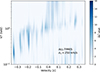 |
Fig. A.1. CIE model scan performed on the time-averaged data, adopting a velocity dispersion of 250 km/s, to address the significance of secondary solutions. |
We also performed simulations for the evaluation of possible secondary peaks in the kT−vLOS maps. Assuming as template the best-fit continuum model plus three cie components (blueshifted, redshifted, and rest-frame) for the time-averaged spectrum (see Table 3), we simulated a new set of RGS and EPIC spectra using the same response files. Then we performed an identical cie scan for these simulated spectra with a velocity dispersion of 250 km/s. Other than the predicted three solutions (±0.3c and rest-frame plasma), we find additional spurious solutions with lower significance (ΔC ≲ 15 or < 2.5σ) at different velocities (0.1 − 0.2c). This means that, although they are describing different features, secondary solutions with low significance (e.g. with < 2.5σ) might partially refer to spurious solutions and we should only consider as robust the results obtained with significance above 2.5σ (ideally > 3σ, see Section 4.4).
Appendix B: Grids of models for photoionised plasmas
In Figs. B.1 and B.2, we show the multidimensional grids for a photoionised plasma in emission and absorption, respectively, obtained for the four analysed datasets (archive-only, time-averaged, and observations 0921360101 and 0921360201) as described in Section 4.3.2. In Figure B.3, we show the contribution of the most significant pion component in the full time-averaged spectrum.
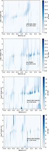 |
Fig. B.1. PIE emission model scan for the four analysed datasets, adopting a velocity dispersion of 250 km/s. The colours show indication of the ΔC-stat improvement compared to the continuum-only model. The black contours refer to significance levels from 2.5 to 3.5σ with steps of 0.5σ estimated with Monte Carlo simulations (see Section 4.4). |
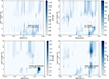 |
Fig. B.2. PIE absorption model scan for the four analysed datasets, using the velocity dispersion that provides the best fit improvement in terms of ΔC-stat. The colours show indication of the ΔC−stat improvement compared to the continuum-only model. The black contours refer to significance levels from 2.5 to 3.5σ with steps of 0.5σ estimated with Monte Carlo simulations (see Section 4.4). |
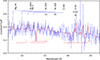 |
Fig. B.3. RGS spectrum in the 7 − 27 Å range, obtained by stacking all XMM-Newton observations. The red curve shows the hybrid ionisation model with two fast, hotter, cie components and a slow, cooler, pion component, on top of the continuum. The rest-frame wavelengths of the most relevant lines are labelled. The dotted (dashed) lines show the velocity shift for the blueshifted (redshifted) lines. The O VII triplet is reproduced by the low-velocity pion component. The data are grouped by a factor of 10. |
All Tables
Best-fit parameters of the cie models applied on the continuum model for the four analysed datasets.
All Figures
|
Fig. 1. Left: Swift/XRT light curve (top) and hardness ratio curve (bottom) of NGC 5204 X-1 from April 2013 to February 2025. The hardness ratio is defined as the ratio between the XRT counts in 3 − 10 keV range and those in 0.3 − 3 keV. The dashed red and green lines indicate the start times of the two latest XMM-Newton observations. Right: Corresponding count rate histogram. |
| In the text | |
|
Fig. 2. EPIC-pn (black), MOS 1 (red), MOS 2 (green), and RGS (blue) spectra and the best-fit continuum model (red curve), from the stacking of all XMM-Newton observations. The continuum emission components are represented by dashed lines in orange (bb) and green (comt). The EPIC data are ignored in the 0.5 − 1.77 keV energy range to employ the full high spectral resolution of RGS and avoid model degeneracy. The EPIC data are grouped according to the optimal binning and, for a better visualisation, the RGS data are grouped by a factor of 9. The bottom panel shows the residuals of the best-fit model. |
| In the text | |
|
Fig. 3. Gaussian line scan performed on the four analysed datasets. We show the results for velocity widths of 2500 km/s (solid grey line) and 100 km/s (dotted blue line). The 3σ threshold (red line) is shown. In the right panel, a zoom in the 0.5 − 0.6 keV energy range is shown to better visualise the O VII line triplet, with the red lines showing the positions of the rest-frame energies. |
| In the text | |
|
Fig. 4. CIE model scan performed on the four analysed datasets, adopting a velocity dispersion of 250 km/s. The colours show indication of the ΔC-stat improvement compared to the continuum-only model. The black contours refer to significance levels from 2.5 to 3.5σ with steps of 0.5σ estimated with Monte Carlo simulations (see Section 4.4). |
| In the text | |
|
Fig. 5. Ionisation balance (top) and stability curve (bottom) for the time-averaged spectra, archive-only data, and new individual observations, using as the SED the best-fit continuum model for each case. Thick blue and red segments show the ranges of the best-fit solutions from the pion and xabs models. |
| In the text | |
|
Fig. 6. Histogram of ΔC-stat values of a CIE model scan of the time-averaged data adopting a velocity dispersion of 250 km/s (blue bars), and of CIE model scans of 5400 Monte Carlo simulated data (red bars). Forecasts for more simulations are made assuming a constant slope of the histogram, in order to visualise different confidence levels. |
| In the text | |
|
Fig. 7. RGS spectrum in the 7 − 27 Å range, obtained by stacking all XMM-Newton observations. The red curve shows the model with three cie components (blueshifted, redshifted, and rest-frame), on top of the continuum. The rest-frame wavelengths of the most relevant lines are labelled. The dotted (dashed) lines show the velocity shift for the blueshifted (redshifted) lines. The data are grouped by a factor of 10. |
| In the text | |
|
Fig. 8. X-ray (0.3 − 10 keV) luminosity, temperature, and velocity dispersion of the cie plasma components as functions of the continuum X-ray luminosity. Filled (empty) red dots show solutions with significance above (below) 2.5σ, and filled black dots are those above 4σ. |
| In the text | |
|
Fig. 9. Zoom on the O VII emission triplet (r: resonance, i: intercombination, f: forbidden; see Section 5.1) as fitted with two sets of three Gaussian lines (red) in the RGS time-averaged spectrum (blue). |
| In the text | |
|
Fig. 10. G (left) and R (right) ratios curves for the O VII triplet. Blue arrows show upper and lower limits, corresponding to lower and upper limits on the temperature, respectively. The dashed black lines indicates the results obtained for the rest-frame O VII triplet, while the dashed blue lines for the blueshifted emission lines. In the right panel, the red point indicates the value of R obtained from the rest-frame O VII lines. |
| In the text | |
|
Fig. A.1. CIE model scan performed on the time-averaged data, adopting a velocity dispersion of 250 km/s, to address the significance of secondary solutions. |
| In the text | |
|
Fig. B.1. PIE emission model scan for the four analysed datasets, adopting a velocity dispersion of 250 km/s. The colours show indication of the ΔC-stat improvement compared to the continuum-only model. The black contours refer to significance levels from 2.5 to 3.5σ with steps of 0.5σ estimated with Monte Carlo simulations (see Section 4.4). |
| In the text | |
|
Fig. B.2. PIE absorption model scan for the four analysed datasets, using the velocity dispersion that provides the best fit improvement in terms of ΔC-stat. The colours show indication of the ΔC−stat improvement compared to the continuum-only model. The black contours refer to significance levels from 2.5 to 3.5σ with steps of 0.5σ estimated with Monte Carlo simulations (see Section 4.4). |
| In the text | |
|
Fig. B.3. RGS spectrum in the 7 − 27 Å range, obtained by stacking all XMM-Newton observations. The red curve shows the hybrid ionisation model with two fast, hotter, cie components and a slow, cooler, pion component, on top of the continuum. The rest-frame wavelengths of the most relevant lines are labelled. The dotted (dashed) lines show the velocity shift for the blueshifted (redshifted) lines. The O VII triplet is reproduced by the low-velocity pion component. The data are grouped by a factor of 10. |
| In the text | |
Current usage metrics show cumulative count of Article Views (full-text article views including HTML views, PDF and ePub downloads, according to the available data) and Abstracts Views on Vision4Press platform.
Data correspond to usage on the plateform after 2015. The current usage metrics is available 48-96 hours after online publication and is updated daily on week days.
Initial download of the metrics may take a while.