| Issue |
A&A
Volume 708, April 2026
|
|
|---|---|---|
| Article Number | A332 | |
| Number of page(s) | 11 | |
| Section | Astrophysical processes | |
| DOI | https://doi.org/10.1051/0004-6361/202558315 | |
| Published online | 21 April 2026 | |
A high-resolution X-ray view of the ultra-fast outflow in MAXI J1810−222
1
INAF – IASF Palermo, Via U. La Malfa 153, I-90146 Palermo, Italy
2
Department of Physics, Ehime University, 2-5, Bunkyocho, Matsuyama, Ehime 790-8577, Japan
3
Univ. Grenoble Alpes, CNRS, IPAG, 38000 Grenoble, France
4
Department of Physics and Astronomy, James Madison University, Harrisonburg, VA, USA
5
Institute of Space Sciences (ICE), CSIC, Campus UAB, Barcelona E-08193, Spain
6
Institut d’Estudis Espacials de Catalunya (IEEC), 08860 Castelldefels (Barcelona), Spain
7
Instituto de Astrofísica de Canarias, E-38205 La Laguna, Tenerife, Spain
8
Departamento de Astrofísica, Universidad de La Laguna, E-38206 La Laguna, Tenerife, Spain
★ Corresponding author: This email address is being protected from spambots. You need JavaScript enabled to view it.
Received:
28
November
2025
Accepted:
16
March
2026
Abstract
Context. The Galactic black hole candidate MAXI J1810−222 was recently reported to exhibit a notable absorption spectral feature at around 1 keV in low-resolution X-ray spectra from detectors resembling charge-coupled devices. The feature is typically correlated with the spectral state of the source being stronger in the soft states, as often occurs in the typical Fe K winds of X-ray binaries (XRBs). However, the results have hinted at rather extreme wind velocities of up to ∼0.1 c.
Aims. We requested and obtained an observation with XMM-Newton to take advantage of the ten-fold higher spectral resolution (R = λ/Δλ ∼ 200 − 400) provided by the RGS detector to resolve the lines and break the degeneracy between different models and interpretations.
Methods. We applied state-of-the-art models of plasma in photoionisation equilibrium and multi-phase interstellar medium (ISM). We performed further comparisons with a re-analysis of NICER and NuSTAR data.
Results. The XMM-Newton/RGS spectrum is consistent with the presence of a mildly relativistic wind, confirming the earlier indications obtained with NICER; however, it places tighter constraints on the outflow properties, with the lines being intrinsically broad. The data would then favour magnetically driven winds, although thermal effects might still contribute to mass loading. NuSTAR and XMM-Newton (EPIC) show a further hotter component, indicating a stratified or multi-phase outflow. Fe K spectra taken with calorimetric detectors (e.g. Resolve on XRISM) will enable a high-resolution view of the complex extreme outflow in this source and shed new light on outflow processes in XRBs.
Key words: accretion / accretion disks / X-rays: binaries / X-rays: individuals: MAXI J1810-222
© The Authors 2026
 Open Access article, published by EDP Sciences, under the terms of the Creative Commons Attribution License (https://creativecommons.org/licenses/by/4.0), which permits unrestricted use, distribution, and reproduction in any medium, provided the original work is properly cited.
This article is published in open access under the Subscribe to Open model. This email address is being protected from spambots. You need JavaScript enabled to view it. to support open access publication.
1. Introduction
Black hole (BH) X-ray transients (BHTs) are binary systems composed of a BH accreting matter from a companion star. These objects spend most of their lifetimes in quiescence, where the X-ray luminosity is lower than ∼1032 erg s−1. However, when efficient accretion turns on, an outburst occurs, increasing the observed X-ray luminosity to 1036 − 39 erg s−1. The outburst phase typically last from a few weeks up to several months (see e.g. Tetarenko et al. 2016), although long outbursts lasting several years or even decades have been reported both in BH systems. Examples include GRS 1915+105 (see e.g. Motta et al. 2021; Deegan et al. 2009), GRO J1655−40 (Sobczak et al. 1999), SWIFT J1753.5−0127 (Zhang et al. 2019), as well as in low-mass X-ray binaries (LMXBs) with neutron stars, such as XMMU J174716.1−281048 (Del Santo et al. 2007) and 4U1608−52 (Šimon 2020).
During a typical outburst, the X-ray spectra of BHTs usually show different states, such as the disc-dominated soft state and the Comptonisation-dominated hard state, as well as intermediate states with spectral parameters in between these two canonical states (see e.g. Done et al. 2007 and references therein). It is generally accepted that the soft and hard X-ray spectral components describe two different emitting regions, with the accretion disc dominating in the soft X-ray range and the hot accretion flow (i.e. the corona) in the hard X-ray band (these components have comparable fluxes at around a few keV). However, these two regions are sufficiently close to interact with each other, giving rise to the reflection component due to the hot photons emitted by the corona being reprocessed by the accretion disc (see e.g. García et al. 2020 and references therein).
Equatorial outflows in the form of disc winds are typically observed in disc-dominated states of sources viewed at high inclinations. This may depend on the radial density profile of the wind (the closer the line of sight is to the disc plane, the higher the optical depth, as discussed in Ponti et al. 2012; Parra et al. 2024). X-ray winds are mainly probed through resonant transitions of highly ionised elements that are blue-shifted by Doppler motions with a velocity of a few hundred km/s. This indicates a lower limit on the wind escape radius of the order of 104–105Rg. Here, the thermal motion of ions, due to the irradiation of X-ray photons from the inner disc, is sufficient to unbind them from the gravitational well of the compact object (thermally driven winds; see e.g. Tomaru et al. 2019 and references therein).
During hard states, winds with similar kinematical properties are detected in the optical and near-infrared bands (see e.g. Muñoz-Darias et al. 2019), suggesting that they are persistent and, at least in the most extreme cases, play a role in regulating the accretion flow (see e.g. Muñoz-Darias et al. 2016). However, they are only detectable in the X-ray band under favourable circumstances with respect to the outflow geometry or ionisation balance, suggesting possible stratification or a multi-phase nature (see e.g. Muñoz-Darias & Ponti 2022).
In some BH systems, particularly those with higher wind speeds being claimed, magnetically driven winds have been suggested as a better description due to their small launching radius (Miller et al. 2006; Chakravorty et al. 2016; Fukumura et al. 2017; Datta et al. 2024). The presence of a relativistic outflow in a sub-Eddington (Ṁ < 1 ṀEdd) accreting stellar-mass black hole is considered strong evidence for a magnetically driven process because thermal gradients cannot drive winds faster than a few thousand km/s (see e.g. Done et al. 2018).
Some X-ray binaries have shown evidence of powerful, relativistic, or ultra-fast outflows (UFOs) blowing up to 0.1 − 0.2 c; however, this is commonly observed at luminosities exceeding the Eddington limit, as it occurs in photospheric bursts of accreting neutron stars (see e.g. Pinto et al. 2014; Barra et al. 2025) and ultraluminous X-ray sources (ULXs; see e.g. Pinto & Walton 2023 and references therein). Still, these cases are characterised by extremely soft X-ray spectra that do not fit within the typical spectral state framework of BHT systems and are likely to enable different launching wind mechanisms. Finally, it is worth noticing that UFOs are seen in a significant fraction of active galactic nuclei (AGNs), even at sub-Eddington rates (∼30%; see e.g. Gianolli et al. 2024 and references therein). They often exhibit a cooler component in the soft X-ray band below 2 keV and show correlations between their properties and the underlying X-ray emitting continuum (see e.g. Xu et al. 2024).
MAXI J1810−222 (hereafter J1810) is an X-ray transient discovered in 2018 by MAXI/GSC close to the galactic plane (Negoro et al. 2018). X-ray and radio spectral timing properties provided by follow-up observations with Swift/XRT, Swift/BAT, and ATCA suggested that the source is most likely a new BHT (see also Appendix B for lack of pulsations), possibly located at a large distance (≳8 kpc; see Russell et al. 2022, hereafter R22).
Unlike most BHTs, J1810 was discovered in a soft state and does not seem to follow the canonical hardness-intensity diagram (HID); instead, it goes back and forth from the hard state to the soft state several times (through intermediate states), making this source very peculiar. Surprisingly, since its discovery seven years ago, J1810 has remained active (e.g. Marino et al. 2023b), which makes it a member of the group of quasi-persistent X-ray binaries. In a previous work (Del Santo et al. 2023, hereafter DS23), we exploited the NICER observations of J1810 performed in 2020 and found statistically significant spectral features around 1 keV in almost all spectra. We confirmed that it was not instrumental by finding it also in a stacked spectrum with Swift/XRT and showing that it strongly depends on the spectral state of the source (DS23). The application of models of plasma in photoionisation equilibrium (PIE) allowed us to show that the plasma was outflowing with velocities up to ∼0.1 c, with the speed peaking during the soft states.
Due to the limited spectral resolution of CCD-like spectra, we requested (and received) a 60 ks observation with XMM-Newton. We used it to resolve and identify the spectral features through the reflection grating spectrometer (RGS).
2. Observations and data reduction
In Table 1, we briefly report the main observations used in this work along with the net exposure times. We do not explore the Neil Gehrels Swift Observatory (hereafter, Swift) in detail, as the full archival dataset was employed.
Observations of J1810.
2.1. Swift data
The outburst of MAXI J1810-222 has been regularly monitored by Swift-XRT, according to the telescope visibility. The observations shown in Fig. 1 correspond to the full XRT dataset (target IDs 00011105 and 00016178), obtained between February 2019 and July 2025. All observations were processed using the online Swift-XRT data products generator1, developed by the UK Swift Science Data Centre. This generator relies on the latest software package and calibration files. The light curve was extracted in the 0.5–10 keV energy range, while the hardness ratio was computed using the count rate in the 0.5–2 keV and 2–10 keV bands.
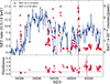 |
Fig. 1. Top panel: Swift/XRT (red diamonds) and Swift/BAT (blue circles) light curves. Bottom panel: XRT hardness defined as the ratio of the counts in the 2–10 keV and 0.5–2 keV energy bands. The dashed line indicates the XMM-Newton observing time. |
We used the Swift-XRT monitoring to trigger the XMM-Newton observation, setting the trigger condition to an observed XRT count rate above ∼4 ct/s and a hardness ratio (2–10 keV/0.5–2 keV) lower than 0.4 (corresponding to high-intermediate and high-soft states). The XMM-Newton observation took place within a week from the trigger time. During the XMM-Newton observation, the XRT 0.5–10 keV count rate was approximately 17 ct/s, which corresponded to either the H1 or H2 (‘high 1/2’) spectra reported in DS23, where fast outflows were observed. During these two high states (soft or soft-intermediate), the temperature of the electron plasma was found to be around 20 keV when using hard X-ray data (see R22).
Data from the Swift-BAT survey were retrieved from the HEASARC public archive and processed using the BAT-IMAGER software (Segreto et al. 2010). This software is specifically designed for the analysis of data from coded-mask telescopes, generating all-sky maps by modelling and subtracting the background. Afterward, light curves and spectra can be extracted for any detected source. For the case of MAXI J1810-222, we derived light curves in the energy range of 15–50 keV, with a time binning of 15 days (Fig. 1). During the XMM-Newton observation, the BAT count rate was very low (i.e. below 1 × 10⁻⁴ ct/s/pixel) consistent with the source being in a soft state.
2.2. XMM-Newton
XMM-Newton observed MAXI J1810−222 on 16 September 2023 for a total exposure time of roughly 61 ks (ObsID 0921250101; P.I.: M. Del Santo). All EPIC instruments were run in TIMING mode with a thick filter. However, we discarded data from MOS1 due to an observation failure. We processed raw data using the Science Analysis System (SAS) version 21.0.02 with most recent calibration files (as of April 2024) and HEASOFT v. 6.34. EPPROC and EMPROC tasks have been used according to standard procedures regarding the patterns (FLAG==0 and PATTERN ≤ 4 (12) for pn and MOS, respectively) and we checked for high particle background periods, which we spotted at the end of the observation. Following the standard threads for EPIC timing mode analysis3, we selected source events from the central 29–47 (278–338) RAWX columns and background events from 3–5 (260–270) columns for pn (MOS2). For diagnostic checks, we also extracted an alternative MOS2 background spectrum from the outer CCDs that collected data in IMAGING mode. We used the SAS tool EPATPLOT to verify that the spectra are not affected by pile-up. We extracted the light curves in two energy bands (0.5–2 and 2–10 keV) and calculated a hardness ratio. No significant flux or spectral variability was observed. Therefore, we extracted an averaged spectrum for the whole observation. The response and ancillary files were extracted with the RMFGEN and ARFGEN tasks.
A preliminary analysis of the pn and MOS2 spectra with simple models (disc blackbody and a power law) revealed instrumental artefacts, possibly due to incorrect background subtraction or incorrect gain or effective area calibration (see Appendix A). After consulting with the XMM-Newton calibration team (Fuerst, priv. comm.), we decided to turn off the default Rate-Dependent PHA (RDPHA) correction (withrdpha = ‘N’) and apply instead the Rate-Dependent CTI (RDCTI) correction, using EPFAST (runepfast = ‘Y’). However, the two methods did not produce any significant difference in the pn spectra; therefore, we kept the standard processed data (i.e. with RDPHA).
In Appendix B, we also describe our search for periodic signals in the high-quality XMM-Newton EPIC-pn data to confirm the non-detection of coherent pulsations in this source. This finding is in agreement with previous results (see e.g. R22 and DS23).
The RGS data reduction was performed with the RGSPROC task, which also extracts spectra and response and area files. We extracted the first-order RGS spectra in a cross-dispersion region of 0.8′ width, centred on the source coordinates and the background spectra by selecting photons beyond the 98% of the source point-spread function. We filtered out periods contaminated by high-background by selecting background-quiescent intervals in the light curves of the RGS 1,2 CCD 9 (i.e. ≳1.7 keV) with a standard count rate below 0.2 cts s−1. The RGS had a net exposure time of 57 ks. Given the consistency between the spectra of the RGS 1 and 2 detectors, we produced a combined RGS spectrum through the RGSCOMBINE task.
2.3. NICER data
The Neutron Star Interior Composition Explorer (NICER; Gendreau et al. 2016) observed the source on two separate days (Obsids 6200560101/0102) on 2023-09-15 and 2023-09-16. We performed the data reduction using NICERDAS software4 version 11, along with NICER CALDB xti20240206.
For each observation, the vast majority of the exposure occurred during orbit ‘day’ periods, which must be analysed independently and include significantly higher background contributions. A proper estimation of that background is only possible with the scorpeon background model and this model requires knowledge of the geomagnetic data during the observations, which we obtained using the NICERDAS task nigeodown.
We first reprocessed the observations using the NICERDAS task nicerl2, separating the orbit ‘day’ and ‘night’ periods and the different orbits, as high differences in calibration and background level require independent analysis. We then filtered for non X-ray flares using a combination of topological and variance based peak detection algorithms. Most notably, instead of the standard static overshoot rate (corresponding to all counts above 20 keV, where the instrument itself has no effective area) threshold of 30 cts/s/FPM, we adopted a dynamical S/N base criterion and only excluded GTI periods with an overshoot rate that is at least five times higher than the 2 − 8 keV count rate (computed on timescales of 1 s). In a second step, we computed the spectral products of each gti period, in the 0.3–10 keV range using nicerl3-spect. To ensure that no significant flare remained in the filtered GTIs (and to assess for any intrinsic variability of the source during the observations), we computed (and visually inspected) the light-curve products obtained using nicerl3-lc, with a 1s binning. The ‘day’ data yield an exposure time of 3.4 ks.
In this work, we avoided performing a new reduction of the archival NICER and NuSTAR data (which are compared with the new NICER and XMM-Newton data in Table 1), but simply retrieved them from previous works (R22 and DS23) to obtain a consistent check of all results.
3. Spectral modelling
For spectral analysis, we used the SPEX fitting package 3.08.01 (Kaastra et al. 1996), which has a full suite of models of line-emitting or absorbing plasmas. The spectra were grouped according to optimal binning (Kaastra & Bleeker 2016) directly in SPEX and fit by minimising the C−statistics (Cash 1979; Kaastra 2017). This binning avoids oversampling the spectra by no more than a factor of 3 with respect to the spectral resolution and requires at least one count per noted bin to satisfy the requirements for the use of the Cash statistics. All uncertainties are reported at the 68% level, which is also the default in SPEX.
3.1. Baseline model
Following DS23, we first focussed on obtaining a reasonable description of the broadband spectral continuum. At first, we modelled the XMM-Newton and NICER (day) spectrum taken between 0.5 keV and 10 keV. The spectral model was fitted simultaneously to the EPIC MOS2/pn, RGS, and NICER spectra with a free multiplicative constant that accounts for the calibration uncertainties. The obvious and well-known mismatch between the EPIC CCD spectra in the timing mode (see also Read et al. 2014), as well as the instrumental artefacts mentioned in Sect. 2.2, forced us to ignore their data below 2.6 keV (RGS and NICER spectral shapes were instead compatible; see Fig. B.1). However, it is important to notice that both the EPIC MOS 2 and pn data still confirm the presence of a strong, broad absorption feature at 1 keV (see Appendix A).
Analogously to the approach in DS23, we adopted a continuum model consisting of a disc-blackbody component (dbb) to account for the soft X-ray emission (peaking below 2 keV) and a Comptonised component (comt) describing the hard X-ray tail. We modelled the photo-electric absorption from the circumstellar and interstellar medium (CSM and ISM) with the hot component, setting the temperature to 10−6 keV to describe a cold neutral gas. All abundances are reported in units of the recently recommended solar abundances of Lodders & Palme (2009), which are default in SPEX. In the SPEX formalism the model reads as follows: hot×(dbb + comt).
The Galactic coordinates of the source (l = 8.77, b = −1.98) and a likely distance of 8 kpc, or larger, imply that our line of sight crosses the inner regions of the Milky Way, where the abundances in the ISM are characterised by a significant gradient (Pinto et al. 2013). We therefore untied the metallicity of the hot component by coupling all elemental abundances to neon (for which we did not expect any depletion from the gas to the dust phase) and keeping the latter as a free parameter in the fit. The seed photon temperature of the comt was coupled to the dbb temperature, while its electron temperature was fixed to 20 keV following the Swift/BAT results for this intermediate-soft state (DS23). Finally, we added an absorbing Gaussian line at 2.2 keV to account for an edge-like feature, most likely due to systematics in the NICER effective area calibration (see e.g. Marino et al. 2023a).
This simple continuum fit is shown in Fig. 2. The disc dbb temperature is around 0.9 keV, while the optical depth of the comt is about 0.4. Assuming a distance of 8 kpc, we measured an intrinsic 0.5–10 keV total luminosity of (9.1 ± 0.3)×1036 erg s−1 (for an observed or absorbed flux of (3.9 ± 0.1)×10−10 erg s−1 cm−2) of which ≳90% is provided by the disc component. The (neutral) ISM has column density, NH, ISM = (7.3 ± 0.1)×1021 cm−2, with a rather high metallicity of about twice the solar value. These results are consistent with DS23. The NICER spectrum shows a strong, broad absorption feature around 1 keV, which is confirmed by the shape of the RGS residuals. The fit statistics for this model are rather poor (C-stat of 1763 for 668 degrees of freedom, hereafter d.o.f.) because we did not yet account for the ionised and dusty phases of the ISM and any XRB winds.
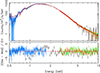 |
Fig. 2. XMM/RGS (blue data) + EPIC (pn/green and MOS2/orange data) + NICER (black data) spectra and best-fit continuum model. EPIC data were ignored below 2.6 keV due to calibration issues. |
3.2. Full ISM model
To employ the high spectral resolution of the RGS, which is needed to accurately model the various interstellar phases and any leftovers due to the XRB winds, we ignored the NICER data in the RGS operating band (i.e. below 1.77 keV). This is a common procedure for different types of source (see e.g. Pinto et al. 2021 and references therein). The NICER spectrum yields a number of counts that is about 0.8 times that obtained with the RGS spectrum and, importantly, at a much lower spectral resolution. Otherwise, we would see degeneracies between the different models, with poor constraints on the line broadening.
A preliminary fit to the spectra with such a low-energy cut for NICER (keeping all abundances coupled to neon, which is free to vary) provided a continuum model with parameters consistent with the previous fit with a C-stat of 1454 for 648 d.o.f.. Since the RGS spectrum resolves the individual interstellar K/L absorption edges, we left the abundances of oxygen, neon, magnesium, silicon, and iron of the hot component free to vary (with all other elements still coupled to neon). The residuals for this model are shown in Fig. 3 (bottom panel, dubbed ‘neutral gas model’). The fit statistics are still poor (C-stat of 1379 for 645 d.o.f.; i.e. ΔC-stat = 75, along with the O, Mg, and Fe abundances left free to vary) for the same reasons as those noted above.
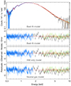 |
Fig. 3. Top two panels: XMM/RGS + EPIC + NICER spectra and best fit model. The NICER (EPIC) data were ignored between 0.5–1.8(2.6) keV to fully employ the high resolving power of RGS and decrease degeneracy between models of line emission and absorption as well as calibration issues. Bottom two panels: Residuals computed for the models without pion and without pion, ISM ions and dust. |
Through visual inspection of the narrow spectral residuals, we identified the 1s − 2p transition energies of O II–IV, O VII–VIII, Ne II–III, and Ne IX–X that are commonly observed in the ISM absorption spectra of X-ray background sources (see e.g. Gatuzz & Churazov 2018 and references therein). We found additional fine structures near the K-edges of oxygen (0.54 keV), neon (0.87 keV), and magnesium (1.31 keV), as well as the L-edge of iron (0.71 keV). The latter could be due to other weaker ionic lines (Ne V–VII), dust (e.g. silicates; Psaradaki et al. 2024; Rogantini et al. 2020) and the photoionised wind previously claimed in this source or in other X-ray binaries (e.g. Pinto et al. 2014).
Following Pinto et al. (2013), we multiplied the continuum model for the slab model in SPEX, which provides a complete set of ionic species for all elements with atomic number from 1 to 30. For both the hot and slab components, we adopted a reliable velocity dispersion of 100 km s−1 (ISM lines are too narrow to be resolved with these data anyway). The column densities were left free in the fit for the slab for the ionic species mentioned above. This enabled the ISM to account for any possible narrow rest-frame spectral feature present in the spectrum because the ionic column densities are not model-dependent. The additional slab component significantly improves the spectral fit (ΔC-stat = 97 for the inclusion of the 11 ionic species).
Finally, we added the contribution from solids, particularly for the modelling of the O, Fe, and Mg edges, using the amol component, which contains a full suite of interstellar equivalents for terrestrial compounds that have been measured in the lab. We used a reliable composition of metallic iron and magnesium silicates (pyroxene, MgSiO3), which so far has provided excellent descriptions of the K- and L-edges in the soft X-ray band (Pinto et al. 2013; Rogantini et al. 2020; Psaradaki et al. 2024). The column densities of these species were free parameters. This provided a major improvement of the edges and overall fit (ΔC-stat/d.o.f. = 37/2).
The spectral residuals for the full ISM model are shown in Fig. 3 (dubbed ‘ISM-only model’). Most narrow features have been taken into account, but there is still a broad feature around 1 keV. The fit statistics (while improved) are still rather poor (C-stat/d.o.f. = 124/632).
3.3. Photoionised plasma
Lastly, we included in the spectral model the photoionised plasma component. This was done using the pion model in SPEX; pion calculates the transmission and emission of a slab of photoionised plasma, where all ionic column densities are linked through a photoionisation model. The relevant parameter is the ionisation parameter ξ = L/nHr2, with L as the source luminosity, nH the hydrogen density, and r the distance from the ionising source. At the moment, this is the only publicly available code that self-consistently computes the balance instantaneously during the spectral fitting. The ionising field or spectral energy distribution (SED) is, therefore the continuum model at each iteration. The final model can be described as follows:

The pion model can be used to produce spectra of PIE plasma both in emission and absorption. We adopted a pure-absorption model by setting a solid angle of Ω/4π = 0 and a covering fraction of fcov = 1. As additional free parameters, we chose the column density, NH, the ionisation parameter, ξ, the line-of-sight velocity, vLOS, and the velocity dispersion or line width, vσ. Given the limited statistics, we assumed solar chemical abundances. This is generally a good approximation of low-count spectra, although might have an impact on the detection of the winds given that their abundances may differ from the solar pattern (see e.g. Barra et al. 2024; Keshet et al. 2024; Kosec et al. 2025).
Since we expected Doppler shifts and wanted to avoid getting stuck within a local minimum, we first performed a scan through model grids of photoionised plasmas for the new NICER+XMM-Newton data, as previously done for the archival NICER data in DS23. We adopted a logarithmic grid of ionisation parameters (log ξ [erg/s cm] between 1 and 6 with 0.2 steps) and vLOS ranging between −0.3 c and +0.1 c. We tested three values of velocity dispersion (vσ = 1000, 10 000 and 20 000 km/s). In Fig. 4, we show the pion scan obtained adopting a velocity dispersion of 20 000 km/s, which provided the largest improvement corresponding to a remarkable Δ C = 72 (for four additional d.o.f.) with respect to the full ISM model. Such a value would correspond to a detection level well above 5σ, even if we take into account the look-elsewhere effect (see e.g. Pinto & Walton 2023 and references therein). Given such a large statistical improvement, we refrained from running specific simulations as it would be redundant. The best-fitting solution was found for log ξ = 2.0 for vLOS = −0.06 c. In addition, weaker structures could also be seen at log ξ ≳ 4, with vLOS below ∼ − 0.1 c, indicating the potential presence of a multi-phase plasma.
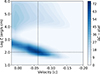 |
Fig. 4. Parameter-space scan throughout model grids of a photoionised plasma in absorption applied onto the XMM-Newton+NICER spectra, adopting a velocity dispersion of 20 000 km/s. The dotted black lines identify the best-fit grid model. Structures are also present at high ξ. |
A direct fit of the data with the pion component in addition to the full ISM model (dubbed the complete or best-fit model) yielded a mildly-relativistic Doppler blueshift of vLOS = −0.061 ± 0.005 c and a consistent broadening of vσ = 0.065 ± 0.005 c. The other two free parameters gave NH = (3.0 ± 0.5)×1021 cm−2 and log ξ = 1.88 ± 0.05 erg s−1 cm. The spectra, best-fit model, and residuals can be found in Fig. 3 (top two panels). Some further very broad continuum-like residuals are still present, most likely due to NICER-XMM-Newton/EPIC cross-calibration issues between 3–5 keV. The results obtained here are in line with those obtained for the intermediate-soft states of this source in DS23. The availability of the high-resolution RGS spectrum enabled us to account for a more complete ISM model (contributing to many rest-frame narrow lines), which resulted in a smaller column density of the pion model with respect to DS23.
3.4. The archival NICER spectra
In DS23, it was shown that the outflow properties were connected to the source spectral state, although the results were obtained by adopting the simple baseline model such as the one used in Sect. 3.1 due to the limited NICER spectral resolution. A meaningful comparison between the results obtained with the archival NICER data and the more recent NICER and, especially, XMM-Newton observations, requires the adoption of an identical spectral model. For this reason, we performed a new fit of the NICER data presented in DS23, which consisted of five flux- and hardness-resolved spectra. The adopted model is consistent with the best-fit model obtained for the new simultaneous NICER and XMM-Newton spectra described in Sect. 3.3. To avoid any degeneracies, we fixed all the parameters of the full ISM model (which are not expected to vary) and the velocity dispersion of the photoionised absorber to the RGS fit results. In addition to the continuum parameter, the only additional free parameters were the column density, the ionisation parameter, and the line-of-sight velocity of the photoionised absorber. In Fig. 5, we compare the results obtained for the NICER archival data (black, filled circles) with those obtained with simultaneous fits of the new data (red, open circles). A final quick test was performed by considering only the new NICER spectrum for comparison with the archival data (see blue star in Fig. 5). The panels refer to the main parameters of the photoionised absorber; the X-axis shows the X-ray luminosity, sorted from softest to hardest spectral states, as described in DS23. H1 and H2 are two high states with different hardness, while LS-LI-LH refer to low states with soft, intermediate and hard spectra. The results are discussed in Sect. 4.
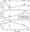 |
Fig. 5. Best-fit parameters of the outflowing plasma component (pion) for the five NICER stacked spectra sorted according to the intrinsic (unabsorbed) X-ray 0.3–10 keV luminosity (re-fit of the flux-resolved spectra with the RGS ISM model) as compared with the new RGS (open red circles) and NICER-only (blue star) results. The X-axis is inverted following the HID evolution from high-soft to low-hard states. |
3.5. The archival NuSTAR spectrum
Unfortunately, there is only one observation taken with this telescope to date and it corresponds to a high-soft state. This soft state spectrum was studied by R22 who focussed their study on the spectral continuum. We noticed some residuals around 8 keV, which pushed us to further investigate the same spectra to understand whether that feature could be related to the presence of any outflows. The NuSTAR FPM A/B spectra are shown in Fig. 6 (upper panel). At first, we fit data from 3 to 20 keV, where the source is above the background and (as above) grouping the spectra with optimal binning in SPEX. The adopted continuum model was the baseline model (disc-blackbody + Comptonisation) introduced in Sect. 3.1. The residuals to the baseline model are shown in the fourth panel (from top to bottom). Absorption features can be seen between 7.5 and 8.5 keV. The multi-phase ISM produces narrow lines predominantly below 3 keV, which allows us to adopt a simple model with only neutral gas for the fit of the NuSTAR spectrum.
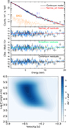 |
Fig. 6. Top panel: NuSTAR spectrum (the only one available) for the soft-intermediate state with alternative models. Bottom panel: Model scan for photoionised plasma in absorption applied onto the NuSTAR spectrum for a velocity dispersion of 20 000 km/s. |
Motivated by the results obtained with the archival NICER data and the RGS confirmation of the detection, we performed a series of model grids for the NuSTAR spectra. We used the pion code in SPEX, which instantaneously computes the photoionisation balance, using the current continuum model as radiation field. As in Sect. 3.3, we adopted a logarithmic grid of ionisation parameters (log ξ [erg/s cm] between 2 and 6 with 0.2 steps) and vLOS ranging between −0.3 c and zero. We tested three values of velocity dispersion (vσ = 1000, 10 000 and 20 000 km/s). In Fig. 6 (bottom panel), we show the pion scan obtained adopting a velocity dispersion of 20 000 km/s in agreement with the XMM-Newton/RGS results. A broad core with vσ= 20 000 km/s provides the largest improvement with Δ C = 23, which corresponds to about 3.0σ, if we take into account the look-elsewhere effect (see e.g. Pinto & Walton 2023 and references therein). The best fit was achieved for vσ = 0.05 ± 0.02 c, vLOS = −0.11 ± 0.02 c, and log ξ = 5.0 ± 0.5 and NH = (1.0 ± 0.5)×1024 cm−2.
In Fig. 6 (second and third panels from top to bottom), we also show the NuSTAR FPM A/B spectral residuals computed for two alternative models using a single plasma phase with large velocity dispersion (as obtained from the pion scan) and a two-phase absorber consisting of two pion components with lower broadening (≲1000 km/s), along with all parameters coupled with the exception of the line-of-sight velocities (vLOS 1, 2 = −0.1 c and −0.15 c, log ξ = 3.6 for a total NH ∼ 2.5 × 1022 cm−2). The use of two narrow-line pion components provides a comparable improvement (Δ C = 26) with respect to the baseline continuum model, most likely due to the limited spectral resolution.
4. Discussion
The discussion is structured as follows. At first, we compare the ISM properties with those in the literature to corroborate our results and obtain some further indication of the source location within the Galaxy. Then we compare the results obtained with different instruments at different epochs. Finally, we provide some more properties of the outflowing plasma and an attempt to understand its nature.
4.1. The ISM along the line of sight
From the hot component describing the cold, neutral, interstellar gas, we can compute the column densities of individual atomic species (for the adopted solar abundances). These can be compared (and summed) with those of ions and solids as measured with the slab and amol components, respectively. By summing up the contributions from each component, we obtained the following abundances in solar units: O/H = Ne/H = 1.5 ± 0.1, Mg/H = 1.6 ± 0.2, Si/H = 1.2 ± 0.3, and Fe/H = 1.2 ± 0.1. Super-solar values are expected for a line of sight that crosses the Galactic inner regions due to the metallicity gradient, but our estimates exceed by about 20% those found in sources at distances below 8 kpc from the Sun (Pinto et al. 2013; Zeegers et al. 2019). This would confirm a larger distance for J1810 that was previously suggested by R22, using the Galactic mass density model of low-mass XRBs (Grimm et al. 2002) as implemented in Atri et al. (2019), and by DS23 (about 20–30 kpc), based on the estimation of the accretion rate of 0.1 ṀEdd.
Comparing the column densities of each element or ion as obtained from the various components, we estimated that the oxygen is roughly distributed as follows: 10 − 15% in solids, 75 − 80% in the neutral phase, 10 − 15% in the low-ionisation (O II–IV) phase, and 5 − 10% in the high-ionisation (O VII–VIII) phase. The ratios between the gaseous phases are consistent for oxygen and neon (the latter is not depleted into solids). For heavier elements, we find a larger depletion with solids contributing to approximately 40 − 50% of neutral iron and, at least, 80% and 90% of magnesium and silicon, respectively. Our results on ionic fractions and dust depletion are fully consistent with recent results on several samples of Galactic XRBs (see e.g. Pinto et al. 2013; Zeegers et al. 2019; Rogantini et al. 2020; Psaradaki et al. 2024). This also implies that we do not find evidence of further narrow absorption lines from slow-moving plasma in the circumstellar medium around J1810.
4.2. Comparison between different epochs
J1810 was discovered as a soft X-ray transient in 2018. Since then, it has been randomly moving from soft (disc-dominated) to hard (corona-dominated) states by passing through intermediate states, where both the disc and the corona contributed significantly to the observed bolometric flux (see Fig. 1 in R22 and Fig. 2 in DS23).
DS23 discovered evidence for a strong 1 keV absorption feature that was more prominent in the soft states. Using with a photoionisation model to interpret this feature, indicating fast outflows and achieving 0.1 c in the soft states. Our simultaneous observations successfully triggered with XMM-Newton and NICER caught J1810 in a high-soft state with a typical disc temperature of about 1 keV and less than 10% of the 0.3 − 10 keV flux provided by the Comptonisation, where we would have expected a strong 1 keV line. This was indeed confirmed in all instruments, including XMM-Newton EPIC (despite some calibration issues for the latter; see Figs. 2 and B.1). A deep exploration of the (ξ, vLOS) parameter space was performed with photoionisation models and confirmed previous results obtained with archival data, but it also places a strong constraint on the line broadening or velocity dispersion and LOS velocities (of about 6% of the speed of light for both). This was not within the reach of the archival data, as only X-ray gratings are currently able to resolve spectral features in the soft X-ray band (0.3 − 2 keV; see Fig. 4). This was also corroborated by the application of a comprehensive and up-to-date ISM absorption model (see Fig. 3). We emphasise that if the 1 keV line was composed of several absorption features, on the one hand, they would be distinguished with the RGS; on the other hand, they would have been easily fitted through the slab model.
For a comparison with different epochs, we performed a new modelling of the archival NICER flux and hardness resolved spectra that were first published in DS23. The results obtained for the new NICER + XMM-Newton data generally agree with those shown by the same high-to-intermediate-soft spectral state with the exception of the outflow velocity, which was lower by a factor of 2–3 in the new data (see Fig. 5). This indicates some evolution of the outflow (the H2 archival spectrum was obtained by averaging NICER spectra with similar flux and hardness levels). This was confirmed by the broad agreement between the results obtained with the individual fits of the new NICER and RGS spectra.
Motivated by such a strong detection, we reanalysed the NuSTAR spectrum presented in R22 and noticed a possible absorption feature near 8 keV (see Fig. 6 top panel), which could even have been spotted although not mentioned in that paper. The application of the same photoionisation model and the exploration of the parameter space (ξ, vLOS) enabled the detection at about 3.0σ of an outflowing plasma with a slightly larger speed (0.1 c; see Fig. 6, bottom panel). This would correspond to a canonical UFO as those seen in AGNs at different Eddington ratios whose nature is still highly debated (see e.g. Tombesi et al. 2010; Gianolli et al. 2024). However, the spectral resolution of NuSTAR is not high enough to distinguish between a single broad-core line and multiple narrow lines. The presence of absorption in the Fe K band is confirmed by the EPIC data whose photoionisation grids show a secondary hotter solution with log ξ ∼ 4.5 in Fig. 4. The (ξ, vLOS) map would favour a slow-moving plasma, perhaps even consistent with being at rest, but given the relevance of the background above 7 keV in the timing-mode EPIC spectra (see Fig. 3), we refrained from further speculation; however, the comparison between the NuSTAR (2018) and the XMM-Newton (2023) data would indeed suggest an evolution over time. For instance, the NuSTAR observation is characterised by a slightly lower flux (about 50% less in the 3–10 keV shared with XMM-Newton and NICER) and softer SED (the Comptonisation contributes less than 10% to the 3–10 keV flux (i.e. three time less than during the XMM-Newton observation); along with the better data quality around 8 keV, this might have had an impact on the line detectability. Finally, the unavailability of high-resolution data covering the whole X-ray band from 0.3 to 10 keV does not allow us to distinguish between a continuous absorption measure distribution (or a stratified plasma) and a more discrete multi-phase outflow. A simultaneous XMM-Newton RGS + XRISM Resolve observation would be needed to cover such a scope.
4.3. The nature of the outflow
Following previous calculations for the flux- and hardness-resolved spectra performed in DS23, we computed some properties of the outflow from the best-fit solution describing soft X-ray absorption lines (vLOS = −0.061 c, NH = 3.0 × 1021 cm−2 and log ξ = 1.88 erg s−1 cm). From the ionisation parameter definition, we can compute a maximum distance for the photoionised plasma: rmax ∼ Lion/(ξ NH) ∼ 107 RG, where for the gravitational radius, RG, we adopted a typical value of MBH = 10 M⊙. A lower limit on the distance can be obtained from the escape radius, rmin ∼ 2GMBH/v2 = 500 RG. These radii may be used to estimate a range of plasma densities: n H, min ∼ NH/rmax = 5 × 107 cm−3 and  cm−3 (for an adopted volume filling factor of b = 0.1). Such a range of densities, while broad, is comparable with those found with direct (He-like triplets) or indirect (variability) arguments in outflows observed in ULXs (e.g. Pinto & Walton 2023), AGNs (e.g. Xu et al. 2024), and Galactic XRBs (e.g. Psaradaki et al. 2018; Kosec et al. 2024). This estimate is conservatively based on thermal driving, an MHD wind could result in an even smaller radius and larger density.
The outflow rate can be expressed as Ṁ = 4 π R2 ρ v Ω C, where Ω and C are the solid angle and the volume filling factor (or clumpiness), respectively, and R is the plasma distance from the source. The kinetic power of the winds is  , where we used ξ = Lion/nHR2. The largest uncertainties concern the solid angle and the clumpiness. In agreement with former results in DS23, the outflow rate appears mildly super-Eddington (Ṁ ∼ 2 ṀEdd, assuming C = 0.1, otherwise Eddington-limited for C ≲ 0.05). In DS23, it was reported that the outflow could remove most of the material, possibly explaining the transition to low states, where both the accretion and outflow rates are significantly smaller (0.1–0.2 ṀEdd). Moreover, such a value would still require an accretion rate of 0.1 ṀEdd, which would correspond to an intrinsic luminosity of 1038 erg/s for a BH, indicating that the source is even more distant at ≳20 kpc (as also suggested in DS23 and R22). For the kinetic power, we obtained L ∼ 0.06 LEdd, which (when taken together with the large outflow rate) could indicate that the mass load is high, thereby slowing down the flow.
The application of the full ISM model (in substitution of a simple neutral gas) confirmed the trend for the parameters of the photoionised plasma as previously obtained in DS23. In particular, while the velocity decreases, the ionisation parameter increases towards the hard state, which is associated to X-ray (0.3 − 10 keV) and bolometric (10−3 − 10 3 keV) luminosities lower by factors of about 5 and 2, respectively, with respect to the hard state. Although this might appear counter-intuitive for ξ, we notice that the strong hardening of the SED may result into a substantial increase in the heating and, therefore, of ξ.
The decrease in the velocity might be investigated in the context of magnetically driven winds. For example, a local heat deposition in the upper layers of the disc gives rise to an enhanced mass loss rate (see e.g. Casse & Ferreira 2000). This extra thermal effect leads to an increase in the load put on the field lines and, thus, a decrease in the wind velocity (which would explain the trend towards the harder states). Alternatively, as the ionising flux increases, the innermost streamlines get ionised first, allowing us to probe more distant outflowing regions; however, a substantial decrease in the column density should be foreseen.
The mildly relativistic velocities as measured for the Doppler shift and broadening in the soft and intermediate states is already a strong indication for magnetic driv. This is due to the fact that in an Eddington-limited regime, the thermal mechanism would be very inefficient in driving outflows significantly above 1000 km/s, as shown by global hydrodynamic simulations (see e.g. Done et al. 2018). The anti-correlation between vLOS and ξ is also not expected in thermal winds, whereas it could be reconciled with MHD scenario of certain density profile (see below for more details as well as the work of Fukumura et al. 2017). In the latter case, for instance, the extra heating on the disc surface (observed during the hard state) would enhance mass loading onto magnetised winds, making it heavier and, thus, slower. Magnetic winds also predict rather broad opening angles with cooler components coming from outer regions, which would then produce visible absorption lines in the case of spectral hardening (see previous comment on probing more distant outflowing regions and also Fig. 5). We notice that such an anti-correlation between vLOS and ξ can also be observed in UFOs detected in AGNs (see e.g. Xu et al. 2021; Gianolli et al. 2024). The description of lower velocities in terms of outer launching regions has also been invoked to explain the appearance of slower outflow components in ULXs (see e.g. Pinto et al. 2020).
The velocity dispersion, as estimated with a single photoionised component, for the cool absorber is rather extreme, even for a magnetic field. This is indeed difficult to achieve as velocity shear unless the flow is very extended (i.e. no clumpiness at odds with recent XRISM results on different sources involving less than a few 1000 km/s). It is plausible that the current value of 20 000 km/s could be masquerading a broad feature behind a sub-structure of multiple, narrow features, similarly to PDS 456 and PG 1211+143 (Xrism Collaboration 2025; Mizumoto et al. 2026). This would falsely imply that the outflow is stratified and extended. XRISM/Resolve resolution at 8 keV (Fe K 0.1 c outflows) exceeds E/dE 1600, which is an improvement over the high-count RGSs at first order at 1 keV by a factor of 8. It is likely that the 1 keV broad feature is a merge of multiple lines with a lower broadening around 1000–2000 km/s, which we cannot fully resolve. Equally good fits can be achieved with a series of narrow PION components (at different LOS velocities; see 2D maps in Fig. 4) just as it occurs for the Fe K region observed with CCDs.
For the column density, NH, to be weakly sensitive with distance, the outflow would need to have a narrow cone and the source to be seen at sufficiently low inclinations. This is expected by the non-detection of slow-moving Fe K thermal winds in the NuSTAR spectrum, the lack of QPOs, and the strong radio RMS versus X-ray RMS (a factor of 10:2, likely due to variable Doppler boosting seen at a low inclination; see R22). More specifically, assuming a continuous density distribution that scales as n ∼ r−p (and ignoring a clumpy nature for simplicity) would result in NH ∼ r(1 − p). Therefore, a shallow density profile around p ∼ 1 would produce NH values that are only weakly sensitive to radius values, allowing for a nearly constant column; this would broadly agree with Fig. 5. Such p values correspond to a large disc ejection efficiency (see e.g. Chakravorty et al. 2016; Datta et al. 2024), which is expected from weakly magnetised discs. Therefore, our results would be consistent with the fact that the outer regions would be weakly magnetised, while the innermost ones would be magnetically saturated, namely in the jet-emitting disc (JED) state. This fits appropriately within the JED-SAD framework (Ferreira et al. 2006; Petrucci et al. 2010; Marcel et al. 2022), where it is assumed that the accretion disc sets in a hybrid magnetic configuration.
4.4. Prospects
As pointed out in Sect. 4.2, we currently lack high-spectral-resolution coverage of the whole 0.3 − 10 keV energy band where most ionic absorption lines from X-ray outflows are expected, which prevents us from obtaining a complete view of the outflow properties. To showcase the capabilities of the XRISM observatory (with closed Resolve gate-valve), we performed a set of simulations for exposure times ranging from 10 to 100 ks. We adopted either the single broad core or the two narrow pion components that provide comparable descriptions of the Fe K blueshifted feature observed in the NuSTAR spectrum (see Sect. 3.5). In Fig. 7 (left panel), we show a XRISM/Resolve simulation (at 5 eV resolution) with the two narrow-line model. The pion absorption lines were removed from the model to highlight the expected residuals, particularly in the intermediate band (2–5 keV). This resembles those produced by the strong outflow observed in GRO J1655–40, which was also interpreted as a magnetic wind (see e.g. Miller et al. 2006).
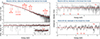 |
Fig. 7. Left panel: XRISM Resolve simulation (40 ks) of J1810 with a photoionised absorption model (two narrow components). Resolve gate-valve closed is adopted. Top-right panel: Resolve simulation with a broad-line model. Bottom-right panel: XRISM Xtend simulation with the broad line model simulation. In both panels, the pion component has been removed to show that the strongest lines are still detected. |
In Fig. 7, in the top-right (bottom-right) panel, we show the residuals to the Resolve (Xtend) spectrum simulated with the broad line model where pion has been removed. For our simulations, we adopted a conservative low-soft state with f2 − 10 keV = 1 × 10⁻¹⁰ erg s−1 cm−2, which represents the lower-flux end of the soft-intermediate states (see also Figs. 1 and 5). In the brighter soft-intermediate states (as for the XMM-Newton data studied in this work), we would expect an even higher flux (up to a factor 3) in the Fe K region. According to our photoionisation calculation, the Fe XXV–XXVI absorption lines (along with some of the sulphur, calcium, and argon lines at lower energies) will remain comparably strong in the intermediate state; meanwhile, in the hard state, the X-ray heating is high enough to fully ionise most ions.
According to our simulations, in a Resolve observation of 40 ks, the pion component produces a spectral improvement ΔC = 60 for the pessimistic case (broad core), corresponding to a confidence level of > 5.0σ (Pinto et al. 2021), which is even higher at a lower velocity dispersion. We expect an accuracy of better than 20% for the pion column density and ionisation parameter, but one that is much smaller for the velocities. This is sufficient to distinguish between the two solutions and measure the outflow kinetic rate. In the pessimistic case, the precision on the S/Fe (Si/Fe or Ar/Fe) abundance ratio will be ∼30% (∼60%). The Xtend data will further corroborate the detection and, importantly, constrain the shape of the broadband spectrum, which is crucial for photoionisation balance calculation.
5. Conclusions
In this work, we performed a high-spectra-resolution study of the notable outflow observed in MAXI J1810-222. The XMM-Newton/RGS spectrum confirmed (with a higher accuracy) the presence of a mildly relativistic wind that was previously suggested by NICER. This would typically favour magnetically-driven winds, although thermal effects may still contribute to mass loading. Measurements of Doppler shifts and velocity dispersion indicate that the lines are intrinsically broad. NuSTAR and XMM-Newton/EPIC spectra also show a further hotter component that produces additional absorption in the Fe K band (7.5 − 8.5 keV) suggesting a stratified or a multi-phase outflow. XRISM observations of J8110 will complement the XMM-Newton/RGS data thanks to an unprecedented view of the Fe K band that will enable the first comprehensive, high-resolution study of the complex extreme outflow in this source and shed new light on outflow mechanisms in XRBs.
Data availability
All data and software used in this work are publicly available from the ESA and NASA Science Archives (https://www.cosmos.esa.int/web/xmm-newton/xsa), (https://heasarc.gsfc.nasa.gov/). Our codes are publicly available on GitHub (https://github.com/ciropinto1982).
Acknowledgments
CP, MDS, AD and FP acknowledge funding from European Union – Next Generation EU, Mission 4 Component 1 CUP C53D23001330006 (PRIN MUR 2022 SEAWIND project No. 2022Y2T94C) and INAF Large Grant 2023 BLOSSOM O.F. 1.05.23.01.13. MDS and AD acknowledge ASI-INAF program I/004/11/6 (Swift). POP, JF acknowledge financial support from the french spatial agency CNES, and from the Action Thématique “Phénomènes Extrêmes et Multimessagers” from the Astronomy & Astrophysics french National Program of CNRS. MP acknowledges support from the JSPS PF for Research in Japan, grant number P24712, and JSPS Grants-in-Aid for Scientific Research-KAKENHI, grant number J24KF0244. T.M.-D. acknowledges support by the Spanish Agencia estatal de investigación via PID2021-124879NB-I00 and PID2024-161863NB-I00. AM is supported by ERC Consolidator Grant “MAGNESIA” No. 817661 and the National Spanish grant PID2023-153099NA-I00.
References
- Atri, P., Miller-Jones, J. C. A., Bahramian, A., et al. 2019, MNRAS, 489, 3116 [NASA ADS] [CrossRef] [Google Scholar]
- Barra, F., Pinto, C., Middleton, M., et al. 2024, A&A, 682, A94 [NASA ADS] [CrossRef] [EDP Sciences] [Google Scholar]
- Barra, F., Barret, D., Pinto, C., et al. 2025, A&A, 694, A266 [NASA ADS] [CrossRef] [EDP Sciences] [Google Scholar]
- Cash, W. 1979, ApJ, 228, 939 [Google Scholar]
- Casse, F., & Ferreira, J. 2000, A&A, 361, 1178 [NASA ADS] [Google Scholar]
- Chakravorty, S., Petrucci, P.-O., Ferreira, J., et al. 2016, A&A, 589, A119 [NASA ADS] [CrossRef] [EDP Sciences] [Google Scholar]
- Datta, S. R., Chakravorty, S., Ferreira, J., et al. 2024, A&A, 687, A2 [NASA ADS] [CrossRef] [EDP Sciences] [Google Scholar]
- Deegan, P., Combet, C., & Wynn, G. A. 2009, MNRAS, 400, 1337 [Google Scholar]
- Del Santo, M., Sidoli, L., Mereghetti, S., et al. 2007, A&A, 468, L17 [NASA ADS] [CrossRef] [EDP Sciences] [Google Scholar]
- Del Santo, M., Pinto, C., Marino, A., et al. 2023, MNRAS, 523, L15 [NASA ADS] [CrossRef] [Google Scholar]
- Done, C., Gierliński, M., & Kubota, A. 2007, A&ARv, 15, 1 [Google Scholar]
- Done, C., Tomaru, R., & Takahashi, T. 2018, MNRAS, 473, 838 [NASA ADS] [CrossRef] [Google Scholar]
- Ferreira, J., Petrucci, P.-O., Henri, G., Saugé, L., & Pelletier, G. 2006, A&A, 447, 813 [NASA ADS] [CrossRef] [EDP Sciences] [Google Scholar]
- Fukumura, K., Kazanas, D., Shrader, C., et al. 2017, Nat. Astron., 1, 0062 [NASA ADS] [CrossRef] [Google Scholar]
- García, J. A., Sokolova-Lapa, E., Dauser, T., et al. 2020, ApJ, 897, 67 [Google Scholar]
- Gatuzz, E., & Churazov, E. 2018, MNRAS, 474, 696 [NASA ADS] [CrossRef] [Google Scholar]
- Gendreau, K. C., Arzoumanian, Z., Adkins, P. W., et al. 2016, SPIE Conf. Ser., 9905, 99051H [NASA ADS] [Google Scholar]
- Gianolli, V. E., Bianchi, S., Petrucci, P.-O., et al. 2024, A&A, 687, A235 [NASA ADS] [CrossRef] [EDP Sciences] [Google Scholar]
- Grimm, H.-J., Gilfanov, M., & Sunyaev, R. 2002, A&A, 391, 923 [NASA ADS] [CrossRef] [EDP Sciences] [Google Scholar]
- Kaastra, J. S. 2017, A&A, 605, A51 [NASA ADS] [CrossRef] [EDP Sciences] [Google Scholar]
- Kaastra, J. S., & Bleeker, J. A. M. 2016, A&A, 587, A151 [NASA ADS] [CrossRef] [EDP Sciences] [Google Scholar]
- Kaastra, J. S., Mewe, R., & Nieuwenhuijzen, H. 1996, in UV and X-ray Spec. of Astr. and Lab. Plasmas, eds. K. Yamashita, & T. Watanabe, 411 [Google Scholar]
- Keshet, N., Behar, E., & Kallman, T. R. 2024, ApJ, 966, 211 [Google Scholar]
- Kosec, P., Rogantini, D., Kara, E., et al. 2024, ApJ, 972, 32 [NASA ADS] [CrossRef] [Google Scholar]
- Kosec, P., Brenneman, L., Kara, E., et al. 2025, ApJ, submitted [arXiv:2510.07615] [Google Scholar]
- Lodders, K., & Palme, H. 2009, Meteorit. Planet. Sci. Suppl., 72, 5154 [Google Scholar]
- Marcel, G., Ferreira, J., Petrucci, P.-O., et al. 2022, A&A, 659, A194 [NASA ADS] [CrossRef] [EDP Sciences] [Google Scholar]
- Marino, A., Russell, T. D., Del Santo, M., et al. 2023a, MNRAS, 525, 2366 [NASA ADS] [CrossRef] [Google Scholar]
- Marino, A., Russell, T. D., Savard, K., Carotenuto, F., & Del Santo, M. 2023b, ATel, 16154, 1 [Google Scholar]
- Miller, J. M., Raymond, J., Fabian, A., et al. 2006, Nature, 441, 953 [NASA ADS] [CrossRef] [Google Scholar]
- Mizumoto, M., Reeves, J. N., Braito, V., et al. 2026, ApJ, 997, 219 [Google Scholar]
- Motta, S. E., Kajava, J. J. E., Giustini, M., et al. 2021, MNRAS, 503, 152 [Google Scholar]
- Muñoz-Darias, T., & Ponti, G. 2022, A&A, 664, A104 [NASA ADS] [CrossRef] [EDP Sciences] [Google Scholar]
- Muñoz-Darias, T., Casares, J., Mata Sánchez, D., et al. 2016, Nature, 534, 75 [Google Scholar]
- Muñoz-Darias, T., Jiménez-Ibarra, F., Panizo-Espinar, G., et al. 2019, ApJ, 879, L4 [CrossRef] [Google Scholar]
- Negoro, H., Nakajima, M., Sakamaki, A., et al. 2018, ATel, 12254, 1 [NASA ADS] [Google Scholar]
- Parra, M., Petrucci, P.-O., Bianchi, S., et al. 2024, A&A, 681, A49 [NASA ADS] [CrossRef] [EDP Sciences] [Google Scholar]
- Petrucci, P. O., Ferreira, J., Henri, G., Malzac, J., & Foellmi, C. 2010, A&A, 522, A38 [NASA ADS] [CrossRef] [EDP Sciences] [Google Scholar]
- Pinto, C., & Walton, D. J. 2023, in Ultra-Luminous X-Ray Sources: Extreme Accretion and Feedback, eds. C. Bambi, & J. Jiang (Singapore: Springer Nature), 345 [Google Scholar]
- Pinto, C., Kaastra, J. S., Costantini, E., & de Vries, C. 2013, A&A, 551, A25 [NASA ADS] [CrossRef] [EDP Sciences] [Google Scholar]
- Pinto, C., Costantini, E., Fabian, A. C., Kaastra, J. S., & in’t Zand, J. J. M. 2014, A&A, 563, A115 [NASA ADS] [CrossRef] [EDP Sciences] [Google Scholar]
- Pinto, C., Walton, D. J., Kara, E., et al. 2020, MNRAS, 492, 4646 [Google Scholar]
- Pinto, C., Soria, R., Walton, D. J., et al. 2021, MNRAS, 505, 5058 [NASA ADS] [CrossRef] [Google Scholar]
- Ponti, G., Fender, R. P., Begelman, M. C., et al. 2012, MNRAS, 422, L11 [NASA ADS] [CrossRef] [Google Scholar]
- Psaradaki, I., Costantini, E., Mehdipour, M., & Díaz Trigo, M. 2018, A&A, 620, A129 [NASA ADS] [CrossRef] [EDP Sciences] [Google Scholar]
- Psaradaki, I., Corrales, L., Werk, J., et al. 2024, AJ, 167, 217 [NASA ADS] [CrossRef] [Google Scholar]
- Read, A. M., Guainazzi, M., & Sembay, S. 2014, A&A, 564, A75 [NASA ADS] [CrossRef] [EDP Sciences] [Google Scholar]
- Rodríguez Castillo, G. A., Israel, G. L., Belfiore, A., et al. 2020, ApJ, 895, 60 [Google Scholar]
- Rogantini, D., Costantini, E., Zeegers, S. T., et al. 2020, A&A, 641, A149 [NASA ADS] [CrossRef] [EDP Sciences] [Google Scholar]
- Russell, T. D., Del Santo, M., Marino, A., et al. 2022, MNRAS, 513, 6196 [Google Scholar]
- Segreto, A., Cusumano, G., Ferrigno, C., et al. 2010, A&A, 510, A47 [NASA ADS] [CrossRef] [EDP Sciences] [Google Scholar]
- Šimon, V. 2020, PASJ, 72, 100 [Google Scholar]
- Sobczak, G. J., McClintock, J. E., Remillard, R. A., Bailyn, C. D., & Orosz, J. A. 1999, ApJ, 520, 776 [NASA ADS] [CrossRef] [Google Scholar]
- Tetarenko, B. E., Sivakoff, G. R., Heinke, C. O., & Gladstone, J. C. 2016, ApJS, 222, 15 [Google Scholar]
- Tomaru, R., Done, C., Ohsuga, K., Nomura, M., & Takahashi, T. 2019, MNRAS, 490, 3098 [NASA ADS] [CrossRef] [Google Scholar]
- Tombesi, F., Cappi, M., Reeves, J. N., et al. 2010, A&A, 521, A57 [NASA ADS] [CrossRef] [EDP Sciences] [Google Scholar]
- Xrism Collaboration (Audard, M., et al.) 2025, Nature, 641, 1132 [Google Scholar]
- Xu, Y., Pinto, C., Bianchi, S., et al. 2021, MNRAS, 508, 6049 [NASA ADS] [CrossRef] [Google Scholar]
- Xu, Y., Pinto, C., Rogantini, D., et al. 2024, A&A, 687, A179 [NASA ADS] [CrossRef] [EDP Sciences] [Google Scholar]
- Zeegers, S. T., Costantini, E., Rogantini, D., et al. 2019, A&A, 627, A16 [NASA ADS] [CrossRef] [EDP Sciences] [Google Scholar]
- Zhang, G.-B., Bernardini, F., Russell, D. M., et al. 2019, ApJ, 876, 5 [Google Scholar]
Appendix A: XMM-Newton EPIC calibration issues
In Fig. B.1, we show a simultaneous fit of the XMM-Newton EPIC MOS 2+RGS and NICER spectra. In this preliminary fit we used a simple continuum model consisting of disc-blackbody and Comptonisation, both absorbed by the ISM neutral gas (see Sect. 3.1). No Gaussian lines were included because we wanted to show all instrumental effects. The models are identical for the four spectra with exception of the multiplicative constant, which was fixed to one for NICER and is free for the other spectra.
The NICER spectrum shows the usual edge near 2.2 keV due to mirror calibration. The EPIC MOS 2 and pn spectra show inconsistencies between 1.5 and 2.5 keV due to instrumental lines and calibration issues. The NICER and RGS spectra are consistent. Nonetheless, all instruments highlight absorption around 1 keV. Interestingly, the parameters of the spectral model are consistent within the uncertainties with the baseline model where EPIC data was ignored below 2.6 keV with the exception for the total X-ray luminosity, L0.5−10 keV = (8.6 ± 0.1) × 1036 erg s−1, and the ISM column density, NH, ISM = (5.9 ± 0.1)×1021 cm−2, both slightly smaller.
Appendix B: Search for pulsations
We searched the XMM-Newton EPIC-pn data for periodic signals following the procedure described in Rodríguez Castillo et al. (2020), using the Pulsation Accelerated Search for Timing Analysis (PASTA) software. We corrected the times of arrival (ToAs) of the source events over a grid of ∼10,000 trial values, applying a factor of  . The range explored was 7 × 10⁻⁶ < |Ṗ/P;(s−1)| < 1 × 10⁻¹¹, where Ṗ is the first derivative of the pulsation period (see Rodríguez Castillo et al. 2020 for further details). No significant coherent signals were detected. We derived a 3σ upper limit of < 0.9% on the pulsed fraction (PF), where PF is defined as the semi-amplitude of a sinusoidal modulation divided by the average count rate.
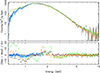 |
Fig. B.1. XMM/RGS (blue data) + EPIC (pn/green and MOS2/orange data) + NICER (black data) spectra and residuals to a simple continuum model. Note EPIC MOS 2 and pn inconsistencies below 2.6 keV. |
All Tables
All Figures
|
Fig. 1. Top panel: Swift/XRT (red diamonds) and Swift/BAT (blue circles) light curves. Bottom panel: XRT hardness defined as the ratio of the counts in the 2–10 keV and 0.5–2 keV energy bands. The dashed line indicates the XMM-Newton observing time. |
| In the text | |
|
Fig. 2. XMM/RGS (blue data) + EPIC (pn/green and MOS2/orange data) + NICER (black data) spectra and best-fit continuum model. EPIC data were ignored below 2.6 keV due to calibration issues. |
| In the text | |
|
Fig. 3. Top two panels: XMM/RGS + EPIC + NICER spectra and best fit model. The NICER (EPIC) data were ignored between 0.5–1.8(2.6) keV to fully employ the high resolving power of RGS and decrease degeneracy between models of line emission and absorption as well as calibration issues. Bottom two panels: Residuals computed for the models without pion and without pion, ISM ions and dust. |
| In the text | |
|
Fig. 4. Parameter-space scan throughout model grids of a photoionised plasma in absorption applied onto the XMM-Newton+NICER spectra, adopting a velocity dispersion of 20 000 km/s. The dotted black lines identify the best-fit grid model. Structures are also present at high ξ. |
| In the text | |
|
Fig. 5. Best-fit parameters of the outflowing plasma component (pion) for the five NICER stacked spectra sorted according to the intrinsic (unabsorbed) X-ray 0.3–10 keV luminosity (re-fit of the flux-resolved spectra with the RGS ISM model) as compared with the new RGS (open red circles) and NICER-only (blue star) results. The X-axis is inverted following the HID evolution from high-soft to low-hard states. |
| In the text | |
|
Fig. 6. Top panel: NuSTAR spectrum (the only one available) for the soft-intermediate state with alternative models. Bottom panel: Model scan for photoionised plasma in absorption applied onto the NuSTAR spectrum for a velocity dispersion of 20 000 km/s. |
| In the text | |
|
Fig. 7. Left panel: XRISM Resolve simulation (40 ks) of J1810 with a photoionised absorption model (two narrow components). Resolve gate-valve closed is adopted. Top-right panel: Resolve simulation with a broad-line model. Bottom-right panel: XRISM Xtend simulation with the broad line model simulation. In both panels, the pion component has been removed to show that the strongest lines are still detected. |
| In the text | |
|
Fig. B.1. XMM/RGS (blue data) + EPIC (pn/green and MOS2/orange data) + NICER (black data) spectra and residuals to a simple continuum model. Note EPIC MOS 2 and pn inconsistencies below 2.6 keV. |
| In the text | |
Current usage metrics show cumulative count of Article Views (full-text article views including HTML views, PDF and ePub downloads, according to the available data) and Abstracts Views on Vision4Press platform.
Data correspond to usage on the plateform after 2015. The current usage metrics is available 48-96 hours after online publication and is updated daily on week days.
Initial download of the metrics may take a while.