| Issue |
A&A
Volume 694, February 2025
|
|
|---|---|---|
| Article Number | A266 | |
| Number of page(s) | 17 | |
| Section | Astrophysical processes | |
| DOI | https://doi.org/10.1051/0004-6361/202452878 | |
| Published online | 19 February 2025 | |
Line detections in photospheric radius expansion bursts from 4U 1820-303
Confirmation of previous detections and their temporal evolution
1
Università degli Studi di Palermo, Dipartimento di Fisica e Chimica, Via Archirafi 36, I-90123 Palermo, Italy
2
Center for Astrophysics | Harvard & Smithsonian, 60 Garden Street, Cambridge, MA 02138, USA
3
INAF/IASF Palermo, Via Ugo La Malfa 153, I-90146 Palermo, Italy
4
Institut de Recherche en Astrophysique et Planétologie, 9 avenue du Colonel Roche, Toulouse 31028, France
5
Department of Physics, University of Texas at Arlington, Arlington, TX 76019, USA
6
Department of Physics and Trottier Space Institute, McGill University, 3600 rue University, Montreal, QC H3A 2T8, Canada
⋆ Corresponding authors; This email address is being protected from spambots. You need JavaScript enabled to view it.
; This email address is being protected from spambots. You need JavaScript enabled to view it.
Received:
4
November
2024
Accepted:
19
December
2024
Abstract
Context. The Neutron star Interior Composition ExploreR (NICER) is the instrument of choice for the spectral analysis of type I X-ray bursts, as it provides high throughput at the X-ray CCD resolution down to 0.3 keV.
Aims. Triggered by the detection of absorption and emission lines in the first four photospheric radius expansion (PRE) bursts detected by NICER, we wish to test the dependence of the absorption line energies on the inferred blackbody radius because it was reported that the absorption line energies were positively correlated with the inferred blackbody radius. This was tentatively explained by a combination of a weaker gravitational redshift and higher blueshifts in a burst with a larger blackbody radius.
Methods. We thus reanalysed these four bursts and analysed another eight bursts from 4U 1820-303, for which we report evidence for PRE. We first followed the spectral evolution of the burst on the shortest possible timescales (tenth of a second). We adopted two parallel continuum descriptions to characterise the photospheric expansion and line evolution. Using the accretion-enhanced model, in which the burst emission is modelled as the sum of a blackbody and a component describing the persistent emission recorded prior to the burst and multiplied by a constant (fa), we inferred maximum equivalent blackbody radii up to ∼900 km. The peak bolometric (0.1–20 keV) luminosity reached between 4 and 7 × 1038 erg s−1 (and even higher when absorption from a putative photoionised absorber is accounted for) in our sample of bursts. This exceeds the Eddington luminosity of a helium accretor. In individual bursts, we detected absorption lines and assessed their significance through extensive Monte Carlo simulations. To characterise the spectral lines, we used dedicated plasma codes available within SPEX with a phenomenological continuum. A deep search throughout the temperature–velocity parameter space was run to explore Doppler shifts and minimise the chance of becoming stuck in local minima.
Results. We detected several significant (> 99.9 % significance) absorption lines, including the 2.97 keV line that was previously reported. We do not confirm the correlation between the line energies and the inferred blackbody radius, but for some bursts with larger radii, up to four lines are reported, and the line strength is higher. From the modelling of the feature lines, a photoionised or collisionally ionised slightly redshifted (almost rest-frame) gas in emission is suggested in most cases. In particular for the burst presenting the greatest PRE, a combination of photoionisation plasma in emission and absorption is preferred, however.
Key words: accretion / accretion disks / stars: neutron / X-rays: binaries / X-rays: bursts / X-rays: individuals: 4U 820-303
© The Authors 2025
 Open Access article, published by EDP Sciences, under the terms of the Creative Commons Attribution License (https://creativecommons.org/licenses/by/4.0), which permits unrestricted use, distribution, and reproduction in any medium, provided the original work is properly cited.
This article is published in open access under the Subscribe to Open model. This email address is being protected from spambots. You need JavaScript enabled to view it. to support open access publication.
1. Introduction
4U 1820-303 is a well-studied type I X-ray burster (Grindlay et al. 1976; Vacca et al. 1986; van Paradijs & Lewin 1987; Haberl et al. 1987; Kuulkers et al. 2002; Strohmayer & Brown 2002; Cumming 2003; Ballantyne & Strohmayer 2004; Güver et al. 2010; Boutloukos et al. 2010; Kuśmierek et al. 2011; in’t Zand et al. 2012; Özel et al. 2016; Suleimanov et al. 2017; Keek et al. 2018; Strohmayer et al. 2019; Galloway et al. 2021). The X-ray binary is located in the globular cluster NGC 6624 at a distance of 8.0 kpc, according to the latest measurements that combine Gaia Early Data Release 3, Hubble Space Telescope, and older data (Baumgardt & Vasiliev 2021). 4U 1820-303 has an orbital period of only 11.4 min, implying that it is a low-mass helium white dwarf companion for the neutron star (Stella et al. 1987). Thus, matter that is accreted onto the neutron star is predominantly helium (e.g. Cumming 2003).
X-ray bursts are very energetic events and are caused by the unstable thermonuclear burning of accreted fuel on the surface of neutron stars (Galloway et al. 2021, for a recent review). 4U 1820-303 shows a wide variety of bursts, from superbursts (Strohmayer & Brown 2002; Ballantyne & Strohmayer 2004) to strong photospheric radius expansion (PRE) bursts (e.g. Keek et al. 2018; Galloway et al. 2017; Suleimanov et al. 2017) and regular bursts (Galloway et al. 2020, and reference therein). From the burst properties, constraints on the mass and radius of the neutron star can be derived (Güver et al. 2010; Kuśmierek et al. 2011; Özel et al. 2016; Suleimanov et al. 2017). Overall, these measurements indicate a rather small radius for the neutron star of about 10 − 12 km, while its mass appears to be on the high side (1.6 M⊙) (Özel et al. 2016). Interestingly, Ballantyne & Strohmayer (2004) followed a 3-hour-long superburst with the Rossi X-ray Timing Explorer (RXTE; Jahoda et al. 1996) and detected a reflection component, whose parameters suggested that the inner disc was pushed away during the event before it recovered its initial state about 1000 seconds later. Using the same RXTE data, in’t Zand & Weinberg (2010) reported evidence for a variable ∼10 keV edge, which they interpreted as the spectral signature of heavy-element ashes expected to be present in thermonuclear X-ray bursts with photospheric superexpansion (Weinberg et al. 2006).
The launch of the Neutron star Interior Composition ExploreR (NICER; Gendreau et al. 2012) offers the unique opportunity to study X-ray bursts, which are very bright events, with a spectral resolution comparable to X-ray CCDs (∼100 eV) and to simultaneously avoid issues such as pile-up. As important, NICER enables us to explore the energy bandpass below 2.5–3 keV, in which the RXTE was not sensitive, and in which the bulk of the blackbody flux is emitted in the PRE phase. In this energy range, the impact of the burst on the accretion disc can also be probed (e.g. Speicher et al. 2022). Finally, the improved spectral resolution of NICER offers unprecedented sensitivity for detecting narrow emission and absorption features (see Degenaar et al. 2018; Galloway et al. 2021, for recent reviews). All this clearly makes NICER the instrument of choice for deep spectral investigations of type I X-ray bursts.
4U 1820-303 is a prototype X-ray burster, and it is therefore not surprising that NICER observed it soon after it was launched and quite intensively afterwards. The first burst observed with NICER showed evidence for PRE (Keek et al. 2018) (see below). This and the subsequent four bursts, three of which showed PRE, were searched for X-ray spectral features by Strohmayer et al. (2019). Combining pairs of bursts showing PRE, Strohmayer et al. (2019) reported a prominent ∼1 keV emission line and two absorption lines at 1.7 and 3 keV, respectively. Strohmayer et al. (2019) interpreted the lines in the context of burst-driven wind models (Yu & Weinberg 2018) and found that the line energies in the co-added spectrum of the first burst pair (which reached larger photospheric radii) appeared to be blueshifted by a factor of 1.046 ± 0.006 compared to the line energies of the second pair of bursts. This was interpreted in a scenario in which pair 1 bursts with the larger radii had weaker gravitational redshifts, but were thought to generate faster outflows and experienced higher blueshifts.
In this paper, we extend the analysis of Keek et al. (2018) and Strohmayer et al. (2019) to a larger sample of 12 bursts present in the NICER archival data of 4U 1820-303, with the goal of searching for more PRE bursts to further investigate the presence of spectral features. We first analyse the data with the so-called enhanced-accretion model (hereafter referred to as fa model) following Worpel et al. (2013), over the shortest possible timescales (a few tenths of a second). We then focus on the spectral analysis of the time interval of the burst, during which the inferred blackbody radius was larger than 100 km, as derived from the fa model. We repeat the analysis with the fa model with the code XSPEC (Arnaud 1996) using its Python wrapper PyXSPEC (Sect. 2). Then the residuals are searched for absorption edges that may be best detected during the PRE phase of the burst. Finally, we characterise the spectral lines with models of optically thin plasmas with advanced models available in SPEX (Sect. 3). In all spectral fits, we adopt Cash statistics (C-STAT; Cash 1979) and optimal spectra binning (Kaastra & Bleeker 2016).
2. Extraction of the spectra, and modelling the burst continuum
We retrieved all the archival data of 4U 1820-303 from HEASARC up to December 2021 and processed them with standard filtering criteria with the nicerl2 script provided as part of the HEASOFTV6.31.1 software suite, as recommended from the NICER data analysis web page (NICER software version : NICER_2022-12-16_V010a). Similarly, the latest calibration files of the instrument were used throughout (the reference from the CALDB database is xti20221001). A systematic error of 1.5% was added, as suggested by the NICER data analysis web page.
The cleaned light curves from each ObsID were produced with nicerl3 between the 0.3 and 7 keV band, with a time resolution of 120 ms, and were searched for X-ray bursts using a standard scanning technique (searching deviations above a local mean). Over the archival data set, seven more bursts were detected (see Table 1) in addition to those reported by Keek et al. (2018), Strohmayer et al. (2019).
Results of the best-fit continuum modelling of the persistent emission with the TBabs*(diskbb+powerlaw) model in XSPEC.
2.1. Persistent emission before the burst
We first extracted a spectrum of the persistent emission through nicerl3 with a 200-second exposure over an interval ending 10 seconds before the onset of the burst (in two cases, the segment was shortened to ∼60 seconds as the burst occurred at the start of the observations). The spectra were grouped with the recommended optimal binning (ftgrouppha,Kaastra & Bleeker 2016)1. The overall spectral shape of the persistent emission combines a soft and a harder component. The persistent emission spectrum was modelled in XSPEC as the sum of an absorbed disc blackbody and a power law. Alternative models for the hard component, such as a Comptonised component (nthcomp or comptt), provided equally good fits, although the seed photon temperature or the electron temperature cannot be constrained (see Sect. 3 for more details).
We recorded the quality of the fit as the deviation of the C-STAT from the expected value following Kaastra (2017). In order to avoid the fitting to be trapped in local minima, we initialised the fits with 20 random values drawn uniformly within plausible ranges. The best-fit results of the persistent emission recorded prior to the burst are listed in Table 1. To compute the flux and associated errors, we generated a set of 40 parameters from the best-fit values and the covariance matrix. We then set the absorption column to zero within each set of parameters and calculated the flux between 0.1 and 20 keV. The parameters of the persistent emission clearly remain close to each other throughout the burst data set. The 0.1–20 keV unabsorbed luminosity varied between ∼2.0 and ∼6.0 × 1037 erg s−1 (assuming a distance of 8 kpc). These are typical luminosities for the hard spectral state of the source (Bloser et al. 2000) when type I X-ray bursts occur.
2.2. Modelling the burst profile on short timescales with the fa model
We generated a set of spectra over the burst profiles with a varying exposure time to ensure that each spectrum had about 1000 burst counts in addition to the average persistent emission recorded prior to the burst (1000 burst counts are sufficient to constrain the fa model, but still enable us to probe short timescales). The integration timescales of the spectra ranged from tenths of a second at the peak to one second in the tail of the bursts. Following Worpel et al. (2013), the burst emission was modelled as the sum of the persistent emission spectrum multiplied by the so-called fa factor and a blackbody spectrum (fa greater than one suggests that the persistent emission increases during a burst, which is likely caused by the effects of Poynting-Robertson drag on the disc material). In XSPEC terminology, the model was then TBabs×(bbodyrad+fa×(diskbb+powerlaw)).
Because the count rate reached during the burst was extremely high, the background is negligible. The column density and the other parameters of the persistent emission were frozen to the values derived from the pre-burst emission, and only fa and the blackbody parameters were allowed to vary. The blackbody flux was converted into an equivalent radius assuming a source distance of 8 kpc (Baumgardt & Vasiliev 2021). Although the bulk of the burst photons was detected below a few keV for the greatest part of the burst, the blackbody temperature close to touchdown reached a few keV and could therefore only be constrained by including data up to 10 keV. The fit was performed by again considering a constant binning of three channels for the spectra, but we verified that an alternative binning scheme yielded fully consistent results. To avoid trapping of the fit in a local minimum, the first burst spectrum fit was initialised with a sample of 50 input values within plausible ranges. The fit of the subsequent burst spectra always started from the fitted parameters of the previous burst spectrum, but was still shacked around, with 20 input values drawn randomly from plausible ranges.
Ten of the 12 detected bursts showed cleared signs of PRE (see Fig. 1 for one representative event of our sample). Our analysis was similar to the one performed by Keek et al. (2018) on the first burst of the sample. We also tested a different model for the persistent emission composed of an absorbed blackbody (bbody) and a Comptonisation (comptt) component, which was used later on in SPEX; our results are fully consistent with each another. In both analyses, the maximum radius reaches a plateau around 200 km, while the blackbody temperature drops to ∼0.45 keV. Our values of fa are also fully consistent and reach up to ∼8 for this burst. From the peak of the PRE phase to touchdown, we recorded a total bolometric (0.1–20 keV) flux of ∼8 ± 0.1 × 10⁻⁸ erg s−1 cm−2, which is slightly higher than the 7.5 ± 0.1 × 10⁻⁸ erg s−1 cm−2 measured by Keek et al. (2018). For the event presented in Fig. 1, the total 0.1–20 keV bolometric X-ray luminosity reached about 7 × 1038 erg s−1 before it dropped at the peak of the PRE and later returned to its plateau value. During this period, the fa parameter also quickly dropped. All this occurred within ∼0.5 seconds. At a distance of 8 kpc, the source reached a super-Eddington luminosity for a helium accretor (a neutron star with a pure helium photosphere has an isotropic Eddington luminosity of  erg s−1; e.g. Strohmayer & Brown 2002, which translates into 3.1×1038 erg s−1 for an 1.6 M⊙ neutron star with a radius of 12 km).
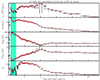 |
Fig. 1. Best-fit parameters of the burst recorded in ObsID 2050300110. From top to bottom: 0.1–20 keV bolometric X-ray luminosity in units of 1038 erg s−1 assuming a 8 kpc distance, the 0.3–10 keV count rate (counts/s), the inferred blackbody radius (km), the blackbody temperature (keV), and the fa parameter. The green area defines the time period during which the inferred blackbody radius was larger than 100 km. All errors are given at the 90% confidence level. |
2.3. Spectral analysis of the burst peak (0.7 second from the peak)
Following Strohmayer et al. (2019), we extracted spectra corresponding to a time interval of 0.7 seconds from the burst peak onwards. We did this by summing the individual ∼1000 count spectra in this time interval. We first fit the spectra with the fa model, and the fit was not acceptable from a statistical point of view for any of the spectra. We modelled the burst emission as the sum of a thermally Comptonised continuum nthcomp model (Zdziarski et al. 1996; Życki et al. 1999), which accounts for the persistent emission, and a blackbody. We set the electron temperature to 10 keV and the seed photon temperature to 0.1 keV. The fit was not acceptable from a statistical point of view either. When we left the column density as a free parameter, the fit improved, but the best-fit value of NH is significantly lower than the value derived from fitting the pre-burst emission inferred from the fa model (∼0.17 versus ∼0.21 ×1022 cm−2). This is problematic and likely due to the fact that the fit tries to compensate for the presence of the unmodelled ∼0.5 keV excess feature identified by Strohmayer et al. (2019). The best-fit parameters of the burst peak spectra fit by the fa model together with the inferred equivalent blackbody radii are listed in Table 2 (freezing the column density to 0.21 × 1022 cm−2). The range of blackbody radii probed by our sample extends significantly over the first five bursts reported by Keek et al. (2018), Strohmayer et al. (2019) and reaches out 900 km.
Results of the continuum modelling for all bursts with the fa model in XSPEC.
Strohmayer et al. (2019) noted that in addition to the 1 keV lines, excess residuals were also present at 0.5–0.6 keV and between 2.0 and 2.4 keV. These excesses were attributed to known unmodelled residuals in the NICER response function at the time their analysis was performed (although we note that no such residuals are present in the persistent emission spectra with the same number of counts). Unmodelled emission lines may artificially create dips in the spectra that in turn may be incorrectly interpreted as absorption lines. The properties of the emission features beyond the 1 keV line therefore need to be investigated first because other emission lines from different species may be present. In order to do this, we scanned the spectrum with a sliding Gaussian over a fixed energy grid and stepped over the normalisation and the width of the Gaussian (in fixed ranges). We performed the scanning iteratively until the improvement in the overall C-STAT did not exceed a critical threshold (set to 8 to begin with). When an excess was detected in this way, a Gaussian function was added to the best-fit model, freeing its energy and its normalisation, but retaining the width from the scan. This improved the C-STAT by a better adjustement of the energy and normalisation of the Gaussian. We assessed the critical threshold of the C-STAT corresponding to a significance higher than 99% through simulations. In addition to the 1 keV line, several other highly significant emission features are detected at ∼2.0 keV and ∼2.5 − 2.6 keV.
The unfolded spectra and associated residuals of the fit for two representative bursts are shown in Fig. 2. The lines reported by Strohmayer et al. (2019) at 1 keV in emission and 3 keV in absorption are clearly visible in the residuals (to improve the statistics, Strohmayer et al. 2019 grouped burst in pairs, but also noted that the lines may be present in individual bursts). The absorption line at 3 keV is also detected in a later observation, when the equivalent blackbody radius was 120 km.
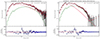 |
Fig. 2. Unfolded spectra of the first burst recorded in ObsID 1050300109 and the burst recorded in ObsID 2050300110. The best-fit model is the sum of an absorbed nthcomp (in red) and blackbody (in dark green) components, with the column density set to 0.21 × 1022 cm−2. The ∼1 keV line and the ∼1.7 and ∼3 keV reported by Strohmayer et al. (2019) are also present in our analysis. |
2.4. Scanning for edges and lines in individual burst peak spectra
There is strong evidence that the 1 keV line reported by Strohmayer et al. (2019) is also present in the subsequent bursts. Before we studied the absorption features, we first added a Gaussian centred around 1 keV with a fixed width (σ = 0.05 keV) to the nthcomp model, and fit the data. The line is statistically significant in several observations, which improves the fit by up to a ΔC-STAT of 25 (and even more for burst 8).
Starting from the best fit, we then scanned the spectra for the presence of additional features in the form of absorption edges or lines. For this purpose, we slid an edge function using the steppar command and allowed depth of the edge (MaxTau parameter) to vary between 0 and 2, sampled with 100 steps. We repeated this for a Gaussian function and allowed the normalisation to vary between −1 and 1 in 100 steps, and we assumed a fixed width (σ = 0.05 keV, consistent with the value reported by Strohmayer et al. 2019). At each energy, we recorded the improvement of the fit through the difference between the C-STAT without any feature and the C-STAT with the emission/absorption feature: the larger the difference, the more significant the feature. We used the centre of the energy bins of each spectrum as the energy grid for the scanning. The results from the Gaussian line scan are shown in Fig. 3. Most spectral scans confirm the 1 keV feature among other features, including some around 2–3 keV. Interestingly, the significance of the 1 keV line is lowest for burst 2 and highest in burst 8, which shows the lowest and highest photospheric expansion by far, respectively.
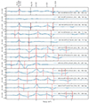 |
Fig. 3. Gaussian line scans for intervals of 0.7 second durations. The best-fit results for the radii expressed in km for a source distance of 8 kpc are obtained with the spectra optimally binned. The best-fit C-STAT and the number of degrees of freedom are given in parenthesis. The lines reported in Strohmayer et al. (2019) are shown as vertical black dash-dotted lines for four of the first five bursts. The position of the local extrema found in the scan are shown with the vertical red lines. |
We do not expect significantly different results for narrower lines widths because the spectral resolution is limited. The line modelling strongly depends on the assumption of emission or absorption, that is, most individual features can be modelled with either emission or absorption lines. We therefore prefer to describe more features simultaneously with plasma models. A more detailed attempt with models of optically thin plasmas is shown in Sect. 3.
2.5. Significance of the detected absorption features
If the detected edge features are not instrumental, their significance remains to be assessed. For this purpose, we followed Hurkett et al. (2008). A covariance matrix evaluated at the best-fit point was used to construct the multivariate Gaussian distribution, from which 1000 parameter values were randomly drawn (using simpars command in XSPEC). For each set of model parameter values, an artificial spectrum was simulated with the appropriate response and ancillary files and exposure time. The counts in each channel were drawn from a Poisson distribution and were binned in the same manner as the observed data. Each simulated spectrum was then fitted and scanned for the presence of a spectral feature in the same way as for the real data. We took bursts 1 and 8 as test cases. None of the simulated spectra showed an improvement of ΔC-STAT larger than 10 in the edge scan, while the maximum value observed in the data reached 13 and 33. This means that the probability that the edge is a spurious feature caused by photon statistics is < 0.1%; and this means that the edge features are detected at > 99.9% confidence. For observation 8, the distribution resulting from the 1000 simulations was scaled to meet the observed ΔC-STAT, and we determined that it would take about 108 − 109 simulations, which is technically unfeasible. However, given the very high ΔC-STAT value for some features (e.g. ∼30 for the 1 keV feature in burst 8), the probability that many of these features are not caused by the noise and look-elsewhere effects still remains very high (≫3σ) when the p value for the number of independent spectral channels is multiplied.
3. Spectral analysis with models of optically thin plasmas
The SPEX fitting package (v3.07.03, Kaastra et al. 1996, 2023) has advanced optically- thin plasma models that may provide further insights into the nature of the lines. As default in SPEX, we assumed that all uncertainties were at the 68% level and grouped the spectra with the recommended optimal binning (Kaastra & Bleeker 2016). For the purpose of studying the behaviour of emission and absorption lines from the bursts, we initially proceeded to describe the continuum model of the spectra. All the models took the absorption from the circumstellar and interstellar medium into account by using the hot model (with a gas temperature of 10−6 keV, which yields a neutral gas phase in SPEX and is equivalent to TBabs in XSPEC). We adopted the most recent solar abundances (Lodders & Palme 2009, default in SPEX) due to the limited spectral resolution and the confusion between the Fe L, Ne K, and Mg K lines with the exception of the oxygen, which was fixed at 1.2 of the solar value, as recommended by the results from high-resolution X-ray spectroscopy (Costantini et al. 2012).
3.1. Testing different spectral models for Obs. 2050300110
First of all, we tested several double-component continuum models for a reasonable description of the spectra before we accounted for the narrow features. In order to do this, we focused on the spectrum of burst 8 (Obs. ID 2050300110), which presents better statistics than the others. In order to avoid degeneracies due to the model, the total column density was set to the value of 1.63 × 1021 cm−2 that was estimated with high-resolution X-ray grating spectrometers (Costantini et al. 2012). The models we tested are combinations of blackbody (bb), multi-temperature disc blackbody (dbb) and inverse Comptonisation of soft photons in a hot plasma (comt) model. The analysis of burst 8 shown that the spectrum is reasonably described with a blackbody bb+comt model (see SPEX manual) with a C-STAT / d.o.f. ∼ 159/57. The temperature of the blackbody is 0.161 keV, to which the temperature of the seed photons of the comt component is coupled.
The optical depth of the comt model was not constrained to the limit of 100 that we imposed, perhaps because the photosphere is optically thick after the expansion and the data are photon-starved above a few keV. The results are shown in Table 3. The best-fit model confirms strong residuals around 1 keV, 2 keV, and 2.6 keV in emission and 3 and 3.4 keV in absorption, and the shape agrees with the XSPEC modelling. These features are analysed in Sect. 4.
Results of the continuum modelling for all bursts with a bb+comt model in SPEX.
3.2. Continuum modelling for the 12 bursts
We proceeded to fit the 12 burst spectra in order to describe the emission and absorption features. The temperature of the blackbody ranged between 0.13 and 0.18 keV (and same range was obtained for the temperature of the comt seed photons). A constraint on the optical depth is difficult to achieve, but in some cases, it was found to be around 13–18 (e.g. in burst 2, where there is no photospheric expansion). The reason probably is that the portion of the photosphere that we observed is optically thick. The best-fit bb+comt model represents the data well, with the exception of the residuals at 1 keV, 2 keV, and 2.6 keV and the absorption features between 3 and 4 keV. This fully agrees with the results obtained through the nthcomp + bbody in XSPEC. We describe these features through plasma models that adopt either collisional-ionisation or photoionisation equilibrium in Sect. 3.3. We show the results of the continuum modelling for all the burst spectra in Table 3. The X-ray and bolometric luminosities are slightly lower than those measured with the power-law models because the latter require stronger curvature in the soft X-ray band, a higher column density and, thereby, higher luminosities. The remarkably higher C-STAT in the spectra with a strong photospheric expansion (and their absence in the persistent spectra) indicates that the features likely have an astrophysical origin and are related to this phenomenology in this way.
3.3. Grids of photo- / collisionally ionised gas
The significance of detecting the plasma component can be enhanced by simultaneously considering multiple spectral lines. To achieve this, we conducted an extensive search across a multi-dimensional parameter space for plasma in photoionisation equilibrium (PIE) and collisional ionisation equilibrium (CIE). One major advantage of this method is that it helps us to avoid the fitting process of becoming trapped in local minima, a common issue when fitting individual lines separately or starting from arbitrary initial parameters. Moreover, this approach facilitates the identification of multiple components or phases within the plasma, which is crucial for an accurate determination of its properties. While this technique can be computationally intensive, we have implemented several strategies to enhance its efficiency, such as varying the plasma model parameters in incremental steps and leveraging pre-calculated model grids to reduce the computational overhead.
3.3.1. Collisionally ionised emitting gas model
As previous done by Kosec et al. (2018) and Pinto et al. (2020b), we performed a multi-dimensional scan with an emission model of a plasma in collisional ionisation equilibrium (cie model in SPEX). CIE plasmas are often observed in stellar coronae and outflows of XRBs (see e.g. Marshall et al. 2002; Pinto et al. 2014; van den Eijnden et al. 2018). We adopted a logarithmic grid of temperatures between 0.1 and 4 keV for a total of 50 bins and line-of-sight velocities, vLOS, between −0.3c and +0.3c (from blueshifted to redshifted plasma, respectively, with a step of 5000 km/s, which is smaller than the spectral resolution in the soft X-ray band). The vLOS was provided by the model red with FLAG = 1, that is, the Doppler rather than the cosmological redshift, which multiplies the cie component. The turbulence of the plasma, vRMS, was fixed to 1000 km/s because Strohmayer et al. (2019) reported it to be around 5000 km/s or lower, and we also wished to avoid intrinsic merging of lines from different ions before convolving with the instrument response. We adopted solar abundances for the cie to avoid an unnecessary model degeneracy and to significantly speed up the computing time. The emission measure defined as EM = nenHV was the only free parameter of the cie model during the spectral fits. We applied this automated routine to scan the cie model grids of the spectra of the 0.7 s bursts. The best-fit results showed a significant improvement, particularly for burst 8, compared to the continuum-only model (ΔC-STATcie = 58). The fit suggests a slight blueshift (vLOS ∼ −0.05c) and a plasma temperature of approximately 1 keV (see Fig. A.1).
3.3.2. Photoionisation plasma in an emission/absorption model
Emission and absorption lines can be generated by winds resulting from photospheric expansion during bursts. These features are modelled using detailed photoionisation calculations, similar to those applied to describe photospheric absorption lines in novae during their supersoft phase (e.g. Pinto et al. 2012; Ness et al. 2022), as well as winds proposed to explain the 1 keV features observed in certain Galactic X-ray binaries (XRBs) and ultraluminous X-ray sources (ULXs) (Del Santo et al. 2023; Barra et al. 2024). These models require an accurate understanding of the radiation field, specifically, of the spectral energy distribution (SED), which spans from optical to hard X-ray wavelengths.
SED and photoionisation balance. As previously done by Pinto et al. (2020a,b), we constructed time-averaged spectra of the bursts from 4U 1820-303 using data from NICER (see Fig. 5). The SED strongly peaks in the X-ray band, which is covered by NICER and restrains any systematic uncertainties in the ionisation balance computation because we know only little about the other energy bands. Therefore, for the X-ray band, that is, 0.3–10 keV, we used the best-fit continuum model bb+comt, as reported in Table 3. A very important parameter of the photoionisation equilibrium is the ionisation parameter ξ = Lion/(nHR2) (see Tarter et al. 1969), where Lion is the ionising luminosity (estimated in the 13.6 eV–13.6 keV range), nH is the hydrogen volume density, and R is the distance from the ionising source. The ionisation balance was calculated with the SPEXpion model, which calculates the transmission and/or the emission of a thin slab of photoionised gas self-consistently. We also computed the stability (or S) curve, which is the relation between the temperature (or the ionisation parameter) and the ratio of the radiation and the thermal pressure, which can be expressed as Ξ = F/(nHckT) = 19 222ξ/T (Krolik et al. 1981). The stability curves are shown in Fig. 7 for the 12 bursts. The branches of the S curves with a negative gradient are characterised by thermally unstable gas, and therefore, the plasma is not expected to be found in their correspondence.
Photoionised plasma in emission. We first describe the emission lines by adding the pion model to the continuum model. In a similar way as for the CIE grids, we created a logarithmic grid with an ionisation parameter log ξ [erg s−1 cm] between 0 and 5 with 0.2 steps and the vLOS from the −0.3c (blueshift) to 0.3c (redshift) with a step of 5000 km/s, and only the pion column density nH was left free to vary. Therefore, we set the pion covering fraction fcov to zero, such that the pion model exclusively produced the emission line, and Ω, the solid angle, equaled 4π (1 in SPEX units). This allowed us to save substantial computational time. For burst 8 (see Fig. B.1), this model produces a similar improvement to that obtained with the cie component (ΔC-STATpion = 55), corresponding to a plasma-redshifted solution with log ξ ∼ 3 and vLOS ∼ 0.02c. However, the solutions obtained with the two different emission models are compatible with a rest-frame solution within a few sigma.
Photoionised plasma in absorption. To conclude, we also conducted a multi-dimensional grid scan using the absorption model. While the pion model is versatile, capable of modelling both emission and absorption, it recalculates the ionisation balance at each iteration, which makes it computationally demanding. For the absorbing gas, we opted for the more efficient xabs model, which is specifically optimised for absorption. This model leverages a pre-calculated ionisation balance from pion, which significantly reduces the computational load. The xabs model shares several parameters with pion, except for the opening angle of the line emission, which is set to zero since no emission is present in this model. We adopted a covering fraction equal to unity in order to avoid degeneracy and to reduce the computing time even further. We calculated the grid of photoionised xabs models in the same way as the pion models, but assuming line-of-sight velocities, vLOS, ranging between −0.3c and zero (i.e. only outflowing gas in absorption or a wind). The best-fit result corresponds to ΔC-STAT ∼ 48 achieved for burst 8 (reported in Fig. C.1) with a log ξ ∼ 2.5 and a velocity vLOS between –0.2c and –0.3c, thereby indicating a blueshifted plasma.
4. Discussion
We focus on the detailed analysis of the bursts in the low-mass X-ray binary 4U 1820-303. Initially, we examine the bursts observed between 2017 and 2021, with particular attention to the occurrence of PRE. Subsequently, we characterize the photospheric expansion and the evolution of spectral lines by employing two parallel continuum descriptions using XSPEC and SPEX, which provided consistent results. Finally, we conduct a thorough analysis of the spectral lines through multi-dimensional scan grids using advanced plasma codes in SPEX, and compare these results with the radii of the PRE bursts.
4.1. Broadband spectral properties
The source 4U 1820-303 exhibits bursts with varying levels of PRE. We conducted an in-depth X-ray spectral analysis of the 0.7-second spectra following the burst peak, focusing on the period when the PRE is at its maximum. Specifically, we performed a dual analysis using two software tools, XSPEC and SPEX. The first tool was employed for spectral feature detection and general spectral modelling, while SPEX was used mostly to model the spectral features with advanced optically thin plasma models. In the various models we tested that took a fixed column density of the cold interstellar gas at 1.63 × 1021 cm−2 (Costantini et al. 2012) into account, our results show that the spectra are described reasonably well with a double-component model composed of a blackbody (bb in SPEX) and a Comptonisation component (comt in SPEX). These take into account the burst and the persistent emission from the source. The temperature of the blackbody is 0.1–0.2 keV and was coupled with the seed photons of the comt component. The optical depth seems unconstrained and ranges between 13 for burst 2 without photosperic expansion and 100, probably because the region of the photosphere that we studied is optically thick and has an electronic temperature between 0.38 and 1.27. The notable C-STAT/d.o.f. is primarily due to emission residuals at 1 keV (Ne X, Fe XXI, and Fe XXII), 2 keV (Si XIV), 2.6 keV (S XVI), and between 3 and 4 keV (Ar XVII) in absorption. This is analysed in the following section. These results agree with those obtained with XSPEC and with the Gaussian line scan reported in Fig. 3. These residuals, which are absent in the persistent spectra or very weak PRE bursts (e.g. burst 2), suggest an astrophysical origin related to the burst phenomena that are discussed in the following section.
4.2. Burst properties
The results of this analysis are consistent with those reported by Yu et al. (2024) for the spectral properties of the bursts, including the blackbody radii. Therefore, we do not discuss these results in further detail here; however, they are included in our description of the component evolution that produces the feature lines (see Sect. 4.3). In order to determine the significance of the detection of the plasma component and its properties, we proceeded with a multi-dimensional scan of model grids of plasmas in photoionised and collisional ionised equilibrium. These are described by pion or xabs models for the photoionised plasma in emission or absorption and cie model, respectively. The plasma components are included in the model once we have obtained a description of the spectral continuum. The results for all burst models are shown in Table D.1 and they are plotted in Fig. D.1. The scan grids for each model and burst, with the corresponding results discussed below, are provided in the appendix.
CIE spectral modelling. The temperature of the plasma component ranges from 1.2 to 1.7 keV, except for bursts 10 and 11, which have a characteristic temperature of approximately 4.4 keV (kTCIE). However, the improvement in their fit to the continuum modelling is equal to or lower than that of the other bursts. The velocity of the emitting plasma is almost the same as the rest-frame velocity within the uncertainties in all the cases. The total X-ray luminosity (0.3–10 keV) associated with the source ranges between (2 − 5)×1038 erg/s, which is slightly higher than the Eddington limit that was forecast for a neutron star of 1.6 M⊙ with a radius of 12 km (∼3.1 × 1038 erg/s, by taking into account that the companion star is a helium white dwarf).
PION spectral modelling. For the pion model, we obtained from modelling the bursts that the plasma moves at low velocities with a temperature of about 1 keV, which is compatible with the complex of Ne X, Fe XXI, and Fe XXII. A deviation from the average values for the column density, the velocity along the LOS, and the ionisation parameter is present for burst 2, which lacks PRE, although these values are compatible within the uncertainties with the results of other modelled bursts. The luminosites of the source lies in the range (2–5)×1038 erg/s, like in the previous case.
XABS spectral modelling. With the xabs model, the improvement in the fit of the burst spectra is approximately ΔC-STAT ∼ 20 compared to the continuum model, with the exception of bursts 6 and 8, where the improvements are ΔC-STAT ∼ 42 and 48, respectively. In these cases, the radius of the blackbody is large (∼122 km and ∼238 km, respectively). For burst 6, a plasma with log ξ ∼ 3 approaching the observer at ∼0.2–0.3c is suggested, which agrees with the results obtained from the other bursts. The luminosites of the source during the bursts is about (2 − 6)×1038 erg/s, although for bursts 1, 3, and 10, a value of 1039 − 40 erg/s is reached due to a high value of the hydrogen column density in the spectral modelling that is most likely affected by systematics because the features are weak.
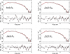 |
Fig. 4. Best-fit spectral modelling of the spectrum of burst 8 with different models. In the upper left panel, the adopted models are bb + comt, (bb + comt)* xabs, bb + comt + cie, and bb + comt + pion. The best-fit results are reported in Tables 3 and D.1. |
Based on the spectral modelling of the emission lines with the cie/pion models, we predict a rest-frame plasma solution, within the uncertainties. When the absorption lines were modelled with the xabs component, the results instead suggest a blueshifted plasma that moves along the LOS, with velocities ranging between ∼(0.2 and 0.35)c. The highest ΔC-STAT variation is obtained for bursts 6 and 8 (which present the highest PRE with respect to the other bursts). For the latter, which presents more statistics, we also tested a pion + xabs component applied to the continuum model. This resulted in a fit with a better quality (C-STAT/d.o.f. ∼ 83/52) than for other all models (ΔC-STAT ≥ 20) and suggests both emitting/absorbing gas with parameters that are compatible with those obtained in Table D.1 (emitting gas: nH,PION ∼ 0.05 ± 0.01 [1024/cm2], vPION ∼ 5706 ± 850 [km/s], log  [erg/s cm]; absorbing gas: nH,XABS = 0.14 ± 0.002[1024/cm2], vXABS ∼ − 99500 ± 700 [km/s], log ξXABS = 2.60 ± 0.01 [erg/s cm]). The best-fit parameters for the plasma are located within the stability region, as shown in Fig. 7 (right panel), except for bursts 1 and 3, whose plasma solutions lie in the instability region (which is characterised by a negative slope). The results obtained with the absorption model, in particular for the velocity of the wind, differs from the results obtained by Yu & Weinberg (2018) and Guichandut et al. (2021). They suggest a wind velocity that is always < 0.1c instead of the 0.2–0.35c that was estimated from our analysis. This may be attributed to the key limitation that the latter analyses are strictly within the context of light-element models, meaning a fully ionised electron-scattering continuum. If a significant amount of metals is present, line-driving could become important and might substantially accelerate the gas to higher velocities such as suggested by our analysis. A challenge in achieving more precise line identifications, beyond the need for higher spectral resolution, is the potential presence of redshifts (in emission, although close to rest-frame in this analysis) and blueshifts (in absorption). These shifts may vary in their contributions for different bursts, as suggested by the results shown in Fig. 6.
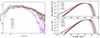 |
Fig. 5. NICER bursts spectral evolution and their SED during time. Left panel: NICER spectra of the 12 bursts (0.7 s exposure time). Right panel: SED of the 12 bursts from the optical to the hard X-rays energy band (0.0001–100 keV). |
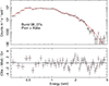 |
Fig. 6. Spectral modelling of the spectrum of burst 8 with the hot * (pion + xabs * (bb + comt)) model. The fit results are reported in the main text. |
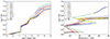 |
Fig. 7. Ionisation balance (left) and thermal stability curves (right) computed for each burst. The regions with thermal instabilities are identified by the segments with negative slopes (right panel). The thicker segments show the ranges of the best-fitting solutions. |
Constraints on the line broadening. We performed two different tests to constrain the line broadening, for which we used the features at 1 keV (in emission) and 3 keV (in absorption) as probes. In the first test, we performed two simulations of the burst 8 spectrum with the same exposure times and based on the best-fit model (continuum + cie; see Fig. 4). The simulations assumed broadening velocities of 1000 km/s and 10 000 km/s, respectively. From the fits of these simulated spectra, we derived an upper limit for the broadening velocity of 5000 km/s in the 1000 km/s simulation case (as found in the original burst 8 dataset), consistent with the spectral resolution. Similar statistical uncertainties were obtained for the 10 000 km/s simulation. These results are compatible within 1–2σ. Additionally, we analysed the absorption feature located at 3 keV (where the resolving power is two to three times higher than the power at 1 keV and the spectrum is less crowded by lines) by fitting it with a Gaussian component in bursts where the line is stronger (e.g. bursts 4, 8, and 11). The derived broadening velocities span the range 3000–40 000 km/s due to their large uncertainties, which are caused by the lower statistics and the still limited resolution at 3 keV. Although strong constraints cannot be placed, the features appear to be intrinsically broadened.
4.3. Lines versus photospheric radius expansion
The burst modelling with the continuum model and the photo-collisional ionisation models shows that the emission/absorption lines are more prominent in burst with a larger PRE (i.e. burst 8, for the residuals at 1 keV). For burst 2, the residuals are instead flat, and this burst lacks a PRE (see the ΔC-STAT improvement in the appendix). Moreover, the intensity of the residuals at 2.2 keV in emission (Si XIV) appears to be correlated with those in absorption at 3 keV (Ar XVII). These results agree with those obtained by Weinberg et al. (2006) and Strohmayer et al. (2019) for the first five burst sorted by ID on Table 2. Simulations indicate that bursts that ignite deep within the neutron star envelope have access to more fuel, which leads to several significant outcomes (Yu & Weinberg 2018). Firstly, the metal synthesis is enhanced and the convection is more intense, which results in a facilitated transport of the nuclear ashes (mainly heavy elements) closer to the photosphere and unveils their distinct spectral signature (in’t Zand & Weinberg 2010 and references therein). During these powerful burst, the luminosity at the base is increased and drives stronger winds, which results in larger photospheric radii. In a following paper, we will examine the correlation between the rapid detection of metals and the intensity of the burst, with a specific focus on the initial rise phase of the burst (following the work done by Yu & Weinberg 2018; Guichandut et al. 2021).
4.4. Bursts versus wind properties in XRBs and ULXs
A useful comparison can be made with the results obtained from photoionisation modelling applied in two different systems, such as MAXI J1810−222 (Del Santo et al. 2023) and Holmberg II X-1 (Barra et al. 2024). In the first case, the strong feature around 1 keV was interpreted as a blend of blueshifted Fe L, Ne X, or O VIII absorption lines. This fact was confirmed by the ion column densities obtained by the xabs component for log ξ ∼ 2. The plasma state solution varies with the spectral state of the source. For the high-flux state, Del Santo et al. (2023) found a highly significant solution of outflowing hot plasma at > 0.1c, which disagrees with the classical Galactic X-ray binary (XRB) thermal winds (with velocities of about 1000 km/s) and invokes strong radiation pressure, such as for winds found in ultraluminous X-ray sources (ULXs; Pinto et al. 2016), although a minimum distance of 100 kpc (outside the Galaxy) is required to identify a source as a ULX. During the soft and intermediate state, the velocity of the plasma is still high for a thermal wind. In the end, for the hard state, the outflow is weaker because the column density is low, and the wind velocity is comparable with wind velocities in XRBs. This variability in the properties of the winds with spectral state might be due to a thermal instability in the plasma or to a different configuration of magnetic field and launching radius. A similar approach was used to model the features in Holmberg II X-1 (Barra et al. 2024). The features in emission at 0.5 keV (N VII) and 0.9 keV (Ne IX) and those in absorption between 0.6 and 0.8 keV and above 1 keV were modelled with photoionisation models (pion and xabs for the emission and absorption lines, respectively). The results of this analysis suggest a multi-phase plasma: The strong N VII emission line (log ξ ∼ 1, v ∼ 0.006c) appears to be distinct from the two hotter absorption and emitting components (log ξ ∼ 3, v ∼ −0.2c). A similar velocity for the absorption lines is required to explain the absorption features in Swift J0243.6+6124 (van den Eijnden et al. 2019). However, an alternative scenario suggests that these features might be linked to iron and magnesium lines, albeit with several caveats. Paczynski & Proszynski (1986) proposed a relativistic model of the wind driven by X-ray bursts and concluded that all the super-Eddington energy flux gently blows out matter, and that the photospheric radius of the outflowing envelope always exceeds 100 km. Yu & Weinberg (2018) supported this with a hydrodynamic simulation of spherically symmetric super-Eddington winds. They demonstrated that the photosphere extends beyond 100 km within the first few seconds, regardless of the burst duration and ignition depth, as shown in Fig. 1.
5. Conclusion
We conducted a comprehensive X-ray spectral analysis of bursts from the low-mass X-ray binary 4U 1820-303 between 2017 and 2021. A model consisting of a blackbody and Comptonisation provided a reasonably good fit for the broadband 0.3–10 keV spectrum, although several features in emission and absorption were evident in the residuals. Specifically, emission lines were detected at 1 keV, 2 keV, and 2.4 keV, while absorption lines appeared at 3 keV and 3.4 keV. These features were interpreted using grids of photo-collisionally ionised gas, suggesting a redshifted (near rest-frame) emitting gas in most cases. Notably, the strength of these lines, in particular, the 1 keV feature, increased with the blackbody radius, indicating that they are linked to astrophysical processes associated with burst phenomena. However, the need for higher spectral resolution leaves open the possibility that both rest-frame emission and blueshifted absorption (with velocities around 20–30% the speed of light) might contribute. Future observations will be crucial to identify these lines more precisely and to define the elements that are involved in these energetic processes with high-resolution (resolving power ≳ 1000) detectors, such as those on board XMM-Newton, Chandra, and XRISM.
Data availability
All the data and software used in this work are publicly available from NASA’s HEASARC archive (https://heasarc.gsfc.nasa.gov/). Our spectral codes and automated scanning routines are publicly available and can be found on the GitHub (https://github.com/ciropinto1982).
Acknowledgments
This work is based on observations obtained with NICER, a NASA science mission funded by the USA. CP acknowledges support for PRIN MUR 2022 SEAWIND 2022Y2T94C funded by European Union – NextGenerationEU and INAF LG 2023 BLOSSOM. T.D.S. acknowledges support from PRIN-INAF 2019 with the project “Probing the geometry of accretion: from theory to observations” (PI: Belloni).
References
- Arnaud, K. A. 1996, in Astronomical Data Analysis Software and Systems V, eds. G. H. Jacoby, & J. Barnes, ASP Conf. Ser., 101, 17 [NASA ADS] [Google Scholar]
- Ballantyne, D. R., & Strohmayer, T. E. 2004, ApJ, 602, L105 [NASA ADS] [CrossRef] [Google Scholar]
- Barra, F., Pinto, C., Middleton, M., et al. 2024, A&A, 682, A94 [NASA ADS] [CrossRef] [EDP Sciences] [Google Scholar]
- Baumgardt, H., & Vasiliev, E. 2021, MNRAS, 505, 5957 [NASA ADS] [CrossRef] [Google Scholar]
- Bloser, P. F., Grindlay, J. E., Kaaret, P., et al. 2000, ApJ, 542, 1000 [NASA ADS] [CrossRef] [Google Scholar]
- Boutloukos, S., Miller, M. C., & Lamb, F. K. 2010, ApJ, 720, L15 [NASA ADS] [CrossRef] [Google Scholar]
- Cash, W. 1979, ApJ, 228, 939 [Google Scholar]
- Costantini, E., Pinto, C., Kaastra, J. S., et al. 2012, A&A, 539, A32 [NASA ADS] [CrossRef] [EDP Sciences] [Google Scholar]
- Cumming, A. 2003, ApJ, 595, 1077 [NASA ADS] [CrossRef] [Google Scholar]
- Degenaar, N., Ballantyne, D. R., Belloni, T., et al. 2018, Space Sci. Rev., 214, 15 [Google Scholar]
- Del Santo, M., Pinto, C., Marino, A., et al. 2023, MNRAS, 523, L15 [NASA ADS] [CrossRef] [Google Scholar]
- Galloway, D. K., & Keek, L. 2021, in Astrophysics and Space Science Library, eds. T. M. Belloni, M. Méndez, & C. Zhang, 461, 209 [NASA ADS] [CrossRef] [Google Scholar]
- Galloway, D. K., Goodwin, A. J., & Keek, L. 2017, PASA, 34 [CrossRef] [Google Scholar]
- Galloway, D. K., in’t Zand, J., Chenevez, J., et al. 2020, ApJS, 249, 32 [NASA ADS] [CrossRef] [Google Scholar]
- Gendreau, K. C., & Okajima, T. 2012, in Space Telescopes and Instrumentation 2012: Ultraviolet to Gamma Ray, eds. T. Takahashi, S. S. Murray, & J. W. A. den Herder, SPIE Conf. Ser., 8443, 844313 [CrossRef] [Google Scholar]
- Grindlay, J., Gursky, H., Schnopper, H., et al. 1976, ApJ, 205, L127 [NASA ADS] [CrossRef] [Google Scholar]
- Guichandut, S., Cumming, A., Falanga, M., Li, Z., & Zamfir, M. 2021, ApJ, 914, 49 [NASA ADS] [CrossRef] [Google Scholar]
- Güver, T., Wroblewski, P., Camarota, L., & Özel, F. 2010, ApJ, 719, 1807 [Google Scholar]
- Haberl, F., Stella, L., White, N. E., Priedhorsky, W. C., & Gottwald, M. 1987, ApJ, 314, 266 [NASA ADS] [CrossRef] [Google Scholar]
- Hurkett, C. P., Vaughan, S., Osborne, J. P., et al. 2008, ApJ, 679, 587 [NASA ADS] [CrossRef] [Google Scholar]
- in’t Zand, J. J. M., & Weinberg, N. N. 2010, A&A, 520, A81 [CrossRef] [EDP Sciences] [Google Scholar]
- in’t Zand, J. J. M., Homan, J., Keek, L., & Palmer, D. M. 2012, A&A, 547, A47 [CrossRef] [EDP Sciences] [Google Scholar]
- Jahoda, K., Swank, J. H., Giles, A. B., et al. 1996, in EUV, X-Ray, and Gamma-Ray Instrumentation for Astronomy VII, eds. O. H. Siegmund, & M. A. Gummin, SPIE Conf. Ser., 2808, 59 [NASA ADS] [CrossRef] [Google Scholar]
- Kaastra, J. S. 2017, A&A, 605, A51 [NASA ADS] [CrossRef] [EDP Sciences] [Google Scholar]
- Kaastra, J. S., & Bleeker, J. A. M. 2016, A&A, 587, A151 [NASA ADS] [CrossRef] [EDP Sciences] [Google Scholar]
- Kaastra, J. S., Mewe, R., & Nieuwenhuijzen, H. 1996, in UV and X-ray Spectroscopy of Astrophysical and Laboratory Plasmas, eds. K. Yamashita& T. Watanabe, 411 [Google Scholar]
- Kaastra, J. S., Raassen, A. J. J., de Plaa, J., & Gu, L. 2023, https://doi.org/10.5281/zenodo.7037609 [Google Scholar]
- Keek, L., Arzoumanian, Z., Chakrabarty, D., et al. 2018, ApJ, 856, L37 [NASA ADS] [CrossRef] [Google Scholar]
- Kosec, P., Pinto, C., Walton, D. J., et al. 2018, MNRAS, 479, 3978 [NASA ADS] [Google Scholar]
- Krolik, J. H., McKee, C. F., & Tarter, C. B. 1981, ApJ, 249, 422 [NASA ADS] [CrossRef] [Google Scholar]
- Kuśmierek, K., Madej, J., & Kuulkers, E. 2011, MNRAS, 415, 3344 [CrossRef] [Google Scholar]
- Kuulkers, E., in’t Zand, J. J. M., van Kerkwijk, M. H., et al. 2002, A&A, 382, 503 [NASA ADS] [CrossRef] [EDP Sciences] [Google Scholar]
- Lodders, K., & Palme, H. 2009, Meteoritics and Planetary Science Supplement, 72, 5154 [NASA ADS] [Google Scholar]
- Marshall, H. L., Canizares, C. R., & Schulz, N. S. 2002, ApJ, 564, 941 [NASA ADS] [CrossRef] [Google Scholar]
- Ness, J. U., Beardmore, A. P., Bezak, P., et al. 2022, A&A, 658, A169 [NASA ADS] [CrossRef] [EDP Sciences] [Google Scholar]
- Özel, F., Psaltis, D., Güver, T., et al. 2016, ApJ, 820, 28 [Google Scholar]
- Paczynski, B., & Proszynski, M. 1986, ApJ, 302, 519 [NASA ADS] [CrossRef] [Google Scholar]
- Pinto, C., Ness, J. U., Verbunt, F., et al. 2012, A&A, 543, A134 [NASA ADS] [CrossRef] [EDP Sciences] [Google Scholar]
- Pinto, C., Costantini, E., Fabian, A. C., Kaastra, J. S., & in’t Zand, J. J. M. 2014, A&A, 563, A115 [NASA ADS] [CrossRef] [EDP Sciences] [Google Scholar]
- Pinto, C., Middleton, M. J., & Fabian, A. C. 2016, Nature, 533, 64 [Google Scholar]
- Pinto, C., Mehdipour, M., Walton, D. J., et al. 2020a, MNRAS, 491, 5702 [Google Scholar]
- Pinto, C., Walton, D. J., Kara, E., et al. 2020b, MNRAS, 492, 4646 [Google Scholar]
- Speicher, J., Ballantyne, D. R., & Fragile, P. C. 2022, MNRAS, 509, 1736 [Google Scholar]
- Stella, L., Priedhorsky, W., & White, N. E. 1987, ApJ, 312, L17 [NASA ADS] [CrossRef] [Google Scholar]
- Strohmayer, T. E., & Brown, E. F. 2002, ApJ, 566, 1045 [NASA ADS] [CrossRef] [Google Scholar]
- Strohmayer, T. E., Altamirano, D., Arzoumanian, Z., et al. 2019, ApJ, 878, L27 [NASA ADS] [CrossRef] [Google Scholar]
- Suleimanov, V. F., Kajava, J. J. E., Molkov, S. V., et al. 2017, MNRAS, 472, 3905 [NASA ADS] [CrossRef] [Google Scholar]
- Tarter, C. B., Tucker, W. H., & Salpeter, E. E. 1969, ApJ, 156, 943 [Google Scholar]
- Vacca, W. D., Lewin, W. H. G., & van Paradijs, J. 1986, MNRAS, 220, 339 [NASA ADS] [CrossRef] [Google Scholar]
- van Paradijs, J., & Lewin, W. H. G. 1987, A&A, 172, L20 [NASA ADS] [Google Scholar]
- van den Eijnden, J., Degenaar, N., Pinto, C., et al. 2018, MNRAS, 475, 2027 [Google Scholar]
- van den Eijnden, J., Degenaar, N., Schulz, N. S., et al. 2019, MNRAS, 487, 4355 [Google Scholar]
- Weinberg, N. N., Bildsten, L., & Schatz, H. 2006, ApJ, 639, 1018 [NASA ADS] [CrossRef] [Google Scholar]
- Worpel, H., Galloway, D. K., & Price, D. J. 2013, ApJ, 772, 94 [NASA ADS] [CrossRef] [Google Scholar]
- Yu, H., & Weinberg, N. N. 2018, ApJ, 863, 53 [CrossRef] [Google Scholar]
- Yu, W., Li, Z., Lu, Y., et al. 2024, A&A, 683, A93 [NASA ADS] [CrossRef] [EDP Sciences] [Google Scholar]
- Zdziarski, A. A., Johnson, W. N., & Magdziarz, P. 1996, MNRAS, 283, 193 [NASA ADS] [CrossRef] [Google Scholar]
- Życki, P. T., Done, C., & Smith, D. A. 1999, MNRAS, 309, 561 [Google Scholar]
Appendix A: CIE grids
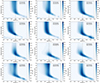 |
Fig. A.1. Multidimensional scan grids with the emission models of collisionally-ionised plasma (cie) for the 12 bursts. |
Appendix B: PION grids
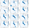 |
Fig. B.1. Multidimensional scan grids with the emission models of photoionised plasma (pion) for the 12 bursts. |
Appendix C: XABS grids
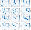 |
Fig. C.1. Multidimensional scan grids with the absorption photo-ionised plasma models (xabs) for the 12 bursts. |
Appendix D: Multi-dimensional scan grids results
Results of the PION - CIE - XABS modelling added to the continuum model for the 12 bursts.
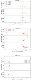 |
Fig. D.1. Results of the grids for the cie (top panel), pion (middle panel) and xabs (bottom panel) modelling. Top panel: LCIE, kTCIE and vLOS vs the total X-ray luminosity. Middle and bottom panel: nH, log ξ and vLOS vs the total X-ray luminosity. The luminosities are estimated in the 0.3-10 keV band. |
All Tables
Results of the best-fit continuum modelling of the persistent emission with the TBabs*(diskbb+powerlaw) model in XSPEC.
Results of the PION - CIE - XABS modelling added to the continuum model for the 12 bursts.
All Figures
|
Fig. 1. Best-fit parameters of the burst recorded in ObsID 2050300110. From top to bottom: 0.1–20 keV bolometric X-ray luminosity in units of 1038 erg s−1 assuming a 8 kpc distance, the 0.3–10 keV count rate (counts/s), the inferred blackbody radius (km), the blackbody temperature (keV), and the fa parameter. The green area defines the time period during which the inferred blackbody radius was larger than 100 km. All errors are given at the 90% confidence level. |
| In the text | |
|
Fig. 2. Unfolded spectra of the first burst recorded in ObsID 1050300109 and the burst recorded in ObsID 2050300110. The best-fit model is the sum of an absorbed nthcomp (in red) and blackbody (in dark green) components, with the column density set to 0.21 × 1022 cm−2. The ∼1 keV line and the ∼1.7 and ∼3 keV reported by Strohmayer et al. (2019) are also present in our analysis. |
| In the text | |
|
Fig. 3. Gaussian line scans for intervals of 0.7 second durations. The best-fit results for the radii expressed in km for a source distance of 8 kpc are obtained with the spectra optimally binned. The best-fit C-STAT and the number of degrees of freedom are given in parenthesis. The lines reported in Strohmayer et al. (2019) are shown as vertical black dash-dotted lines for four of the first five bursts. The position of the local extrema found in the scan are shown with the vertical red lines. |
| In the text | |
|
Fig. 4. Best-fit spectral modelling of the spectrum of burst 8 with different models. In the upper left panel, the adopted models are bb + comt, (bb + comt)* xabs, bb + comt + cie, and bb + comt + pion. The best-fit results are reported in Tables 3 and D.1. |
| In the text | |
|
Fig. 5. NICER bursts spectral evolution and their SED during time. Left panel: NICER spectra of the 12 bursts (0.7 s exposure time). Right panel: SED of the 12 bursts from the optical to the hard X-rays energy band (0.0001–100 keV). |
| In the text | |
|
Fig. 6. Spectral modelling of the spectrum of burst 8 with the hot * (pion + xabs * (bb + comt)) model. The fit results are reported in the main text. |
| In the text | |
|
Fig. 7. Ionisation balance (left) and thermal stability curves (right) computed for each burst. The regions with thermal instabilities are identified by the segments with negative slopes (right panel). The thicker segments show the ranges of the best-fitting solutions. |
| In the text | |
|
Fig. A.1. Multidimensional scan grids with the emission models of collisionally-ionised plasma (cie) for the 12 bursts. |
| In the text | |
|
Fig. B.1. Multidimensional scan grids with the emission models of photoionised plasma (pion) for the 12 bursts. |
| In the text | |
|
Fig. C.1. Multidimensional scan grids with the absorption photo-ionised plasma models (xabs) for the 12 bursts. |
| In the text | |
|
Fig. D.1. Results of the grids for the cie (top panel), pion (middle panel) and xabs (bottom panel) modelling. Top panel: LCIE, kTCIE and vLOS vs the total X-ray luminosity. Middle and bottom panel: nH, log ξ and vLOS vs the total X-ray luminosity. The luminosities are estimated in the 0.3-10 keV band. |
| In the text | |
Current usage metrics show cumulative count of Article Views (full-text article views including HTML views, PDF and ePub downloads, according to the available data) and Abstracts Views on Vision4Press platform.
Data correspond to usage on the plateform after 2015. The current usage metrics is available 48-96 hours after online publication and is updated daily on week days.
Initial download of the metrics may take a while.