| Issue |
A&A
Volume 708, April 2026
|
|
|---|---|---|
| Article Number | L15 | |
| Number of page(s) | 7 | |
| Section | Letters to the Editor | |
| DOI | https://doi.org/10.1051/0004-6361/202558387 | |
| Published online | 17 April 2026 | |
Letter to the Editor
Angular momentum transport through the baroclinic instability in intermediate-mass stars
1
University of Geneva, Department of Astronomy, 51 Ch. Pegasi, CH-1290 Versoix, Switzerland
2
Yunnan Observatories, Chinese Academy of Sciences, Kunming 650216, China
3
Astronomical Institute, Graduate School of Science, Tohoku University, Sendai 980-8578, Japan
★ Corresponding author: This email address is being protected from spambots. You need JavaScript enabled to view it.
; This email address is being protected from spambots. You need JavaScript enabled to view it.
Received:
3
December
2025
Accepted:
5
March
2026
Abstract
Context. Models of rotating stars in which the transport of angular momentum (AM) is only driven by the shear instability and the meridional circulation tend to overestimate the internal degree of radial differential rotation, when compared to asteroseismic observations. This indicates that additional physical recipes are needed to accurately describe AM transport in radiative stellar layers.
Aims. We investigated the transport of AM in intermediate-mass stars through the baroclinic (BC) instability.
Methods. We implemented in the GENeva Evolution Code (GENEC) a formalism to account for the transport of AM through the BC instability. Numerical simulations were then performed for different initial rotation velocities assuming solid-body rotation on the zero-age main sequence, and both with and without this process in addition to the transport by the shear instability and meridional currents.
Results. We find that the inclusion of an additional AM transport process driven by the BC instability is able to counterbalance the creation of radial differential rotation during the evolution on the main sequence. The effects of the BC instability on the rotation profile appear to be stronger for models with a higher initial rotation velocity. The near-core rotation rates and surface rotation velocities predicted by models with the BC instability accurately reproduce the trend in the observed data available for main-sequence γ Doradus stars. AM transport by the BC instability is, however, not efficient enough in later evolutionary stages to reproduce the low core rotation rates observed in the central layers of red giant stars.
Conclusions. The BC instability appears to be an interesting candidate for the unknown process that transports AM in the interior of main-sequence intermediate-mass stars, in particular for γ Doradus stars. However, it is found to be insufficient to correctly account for the internal rotation of red giants.
Key words: methods: numerical / stars: evolution / stars: interiors / stars: rotation
© The Authors 2026
 Open Access article, published by EDP Sciences, under the terms of the Creative Commons Attribution License (https://creativecommons.org/licenses/by/4.0), which permits unrestricted use, distribution, and reproduction in any medium, provided the original work is properly cited.
This article is published in open access under the Subscribe to Open model. This email address is being protected from spambots. You need JavaScript enabled to view it. to support open access publication.
1. Introduction
Thanks to the rapid development of asteroseismic techniques, the internal rotation of intermediate-mass stars can now be determined. In particular, the mean rotation rates of radiative layers that are located at the border of the convective core have been determined for a large number of γ Doradus pulsators (Van Reeth et al. 2016; Ouazzani et al. 2017, 2019; Li et al. 2020; Saio et al. 2021; Aerts et al. 2025). Purely hydrodynamic rotating stellar models that only account for angular momentum (AM) transport through meridional currents and the shear instability have been unable to correctly reproduce these observations; this points towards an unknown additional efficient transport process at work in the radiative interiors of these stars (Ouazzani et al. 2019; Mombarg 2023; Moyano et al. 2023, 2024). In addition to the main-sequence (MS) phase, asteroseismic observations have also enabled the determination of the internal rotation for stars with similar masses as γ Doradus pulsators during the more evolved subgiant and red giant phases Beck et al. (2012), Deheuvels et al. (2012), Mosser et al. (2012), Deheuvels et al. (2014, 2015), Di Mauro et al. (2016), Deheuvels et al. (2017), Triana et al. (2017), Gehan et al. (2018), Tayar et al. (2019), Deheuvels et al. (2020), Li et al. (2024), Dhanpal et al. (2025). Comparisons with core rotation rates predicted by rotating models that solely include AM transport by the shear instability and meridional currents have also shown that these processes lead to an insufficient coupling in stellar radiative zones to account for these observational constraints (e.g. Eggenberger et al. 2012; Ceillier et al. 2013; Marques et al. 2013). This clearly indicates the existence of an efficient AM transport mechanism in addition to meridional circulation and the shear instability for both MS and post-MS stars.
A first possibility to account for this additional AM transport process is related to magnetic instabilities. In particular, the magnetic Tayler instability (Tayler 1973) could play an important role in the internal transport of AM (Spruit 2002). This magnetic transport mechanism, which is referred to as the Tayler-Spruit dynamo, has been found to correctly account for the solar rotation profile (Eggenberger et al. 2005, 2019a, 2022a) but provides an insufficient coupling in the radiative interior of evolved stars to explain the low core rotation rates observed in red giants (Cantiello et al. 2014; den Hartogh et al. 2019). Revised prescriptions for this AM transport by the magnetic Tayler instability have been proposed; they are in better global agreement with observational constraints (Fuller et al. 2019; Eggenberger et al. 2022b; Moyano et al. 2023) but still face difficulties in correctly reproducing the variation in the core rotation rates observed as a function of the evolutionary stage or the mass of the stars (Eggenberger et al. 2019b; den Hartogh et al. 2020; Moyano et al. 2024). The transport of AM in stellar radiative regions can also occur through internal gravity waves. In particular, the AM transport through gravity waves generated by penetrative convection constitutes a promising explanation for the internal rotation of subgiant stars (Pinçon et al. 2017). AM transport by internal gravity waves is, however, found to be insufficient to correctly reproduce the rotation rates observed in the cores of red giant stars (Fuller et al. 2014; Pinçon et al. 2017). Another candidate is the transport of AM by mixed oscillation modes: such a transport mechanism could play an important role in the internal rotation of evolved red giants but is found to be inefficient during the subgiant and the early red giant phases (Belkacem et al. 2015; Bordadágua et al. 2025).
This shows that there is currently no single AM transport mechanism that is able to correctly account for the internal rotation of stars of different masses and at various evolutionary stages. In this context, it is interesting to investigate the potential role of other AM transport processes, and in particular transport by other hydrodynamic instabilities. The present study focuses on the transport of AM through the baroclinic (BC) instability for MS γ Doradus pulsators and more evolved post-MS stars.
2. Modelling of angular momentum transport
Under the assumption of a strong horizontal turbulence, the rotation profile Ω(r, θ, φ) is assumed to only depend on the radius (r), i.e.  . The AM transport in a radiative zone is described as in Zahn (1992):
 (1)
(1)
where ρ stands for the local density, Mr is the mass coordinate at radius r, U(r) is the radial dependence of the vertical component of the meridional currents, and D is the AM transport diffusion coefficient. In standard rotating models computed with the GENeva stellar Evolution Code (GENEC; Eggenberger et al. 2008), the diffusion of AM is performed solely through the secular shear instability such that D = Dshear, with Dshear the diffusion coefficient associated with the transport by this instability, which is taken as in Maeder (1997). The diffusion coefficient for the horizontal turbulence was set as in Zahn (1992). Fujimoto (1987) derived two criteria for stability against non-axisymmetric perturbations, and Fujimoto (1988, 1993) then proposed a prescription for a one-dimensional diffusion coefficient for AM transport driven by the BC instability that reads as
 (2)
(2)
where  is the Richardson number, with N the Brunt-Vaïsälä frequency, and
  is the critical Richardson number for the BC instability. Above this critical Richardson number, the Coriolis effects lead to a decrease in the AM transport efficiency as expressed by the second condition of Eq. (2). The factor αBC in Eq. (2) corresponds to a calibration parameter that accounts for uncertainties in the saturation of the instability. While this prescription for transport by the BC instability has mainly been used in the context of accreting stars by Fujimoto (1988, 1993), its derivation is more general and is valid provided that the key assumption of high Richardson numbers (ℛi ≫ 1) is satisfied. The radiative zones of intermediate-mass stars (both on the MS and the subgiant/early red giant phases) are characterized by Richardson numbers ℛi ≫ 1, so the approach of Fujimoto for the BC instability is well adapted (see Fig. A.2). Note that we did not account for the coefficient for the transport by the Kelvin-Helmholtz (also named dynamical shear) instability (Eq. (26) of Fujimoto 1993), since these high Richardson numbers imply that this instability cannot be triggered. Consequently, only the secular shear instability (and not the dynamical one) was considered in the present study. Radiative zones of intermediate-mass stars were also in the regime of ℛi > ℛiBC (see Fig. A.2), so the vertical length scale on which the BC instability operates is strongly reduced compared to HP, becoming HP(ℛiBC/ℛi)1/2 (Eq. 20 of Fujimoto 1988). The second expression of Eq. (2) was then used for the AM transport.
In the present study, we implemented the diffusion coefficient, Eq. (2), associated with the AM transport by the BC instability in GENEC. For rotating models that account for the effects of the BC instability in addition to meridional currents and the (secular) shear instability, Eq. (1) was solved with a diffusion coefficient for AM transport given by D = Dshear + DBC. This enabled us to compare simulations in which the transport of AM is carried in the classical rotating scheme (i.e. with only the effects of the shear instability and the meridional circulation) to simulations in which AM is transported through the BC instability in addition to the transport by meridional currents and the shear instability.
3. Results
We simulated the evolution of 1.5 M⊙ stars at solar metallicity with initial rotation velocities on the zero-age main sequence (ZAMS) of Vini = 0.2 and 0.4 units of Vcrit (corresponding to equatorial velocities of about 74 and 147 km s−1, respectively). These values are representative of the surface rotation velocities observed for γ Doradus stars and cover most of the observations used in this Letter (see Fig. 2 and Gebruers et al. 2021). The models start at the ZAMS and assume solid-body rotation. This assumption seems justified since, quickly after the ZAMS, the star converges towards the same rotational configuration, independently of its evolutionary history during the pre-MS (see Fig. 13 and Appendix A.1 of Moyano et al. 2023). At first, we computed models in which only the effects of the shear instability and the meridional circulation are considered. We denote these simulations with the term ‘without BC’ in the rest of this Letter. Figure 1 shows the MS evolution of the ratio of core-to-surface rotation rates (Ωc/Ωs) as a function of the central hydrogen mass fraction (Xc) for these models (dashed lines in Fig. 1). Both models show an increasing core-to-surface ratio during their evolution on the MS. However, this increase is more rapid and pronounced at the beginning of the MS for higher initial rotation rates, while the opposite behaviour is observed during the second part of the MS evolution, with higher ratios of core-to-surface rotation rates for models computed with lower initial rotation velocities. The creation of this radial differential rotation is mainly due to the advection of AM by meridional currents at the beginning of the MS and then to changes in the stellar structure during the evolution on the MS: central layers contract, while surface layers expand. The velocity of the meridional circulation increases with the rotation rate of the star, which explains the strongest impact of meridional currents in faster rotating stars, and hence the higher degree of radial differential rotation observed at the beginning of the MS evolution for the Vini = 0.4 Vcrit model without BC in Fig. 1.
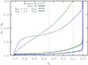 |
Fig. 1. Evolution of the core-to-surface rotation rates as a function of the central hydrogen mass fraction for a 1.5 M⊙ star at solar metallicity. Dashed (solid) lines show the models without (with) the BC instability. The colours differentiate models starting with an initial rotation velocity on the ZAMS of Vini = 0.2 ⋅ Vcrit (green) and Vini = 0.4 ⋅ Vcrit (blue). The vertical lines indicate the evolutionary stages where the rotation profiles are shown in Fig. A.5. |
3.1. Impact of the baroclinic instability on the internal rotation
Simulations were then performed by accounting for the BC instability (‘with BC’) as given by Eq. (2). Following Fujimoto (1993), the numerical factor αBC was first set to a default value of 1.0 for these models, and the impact of using a significantly lower value of 0.001 was studied in a second time (see Appendix B). Figure 1 shows the evolution of the core-to-surface ratio for the ‘with BC’ simulations, where αBC is set to 1.0. In these simulations there is a stronger coupling between the core and the surface; this indicates an efficient AM transport thanks to the BC instability, which is able to counteract the creation of differential rotation. The coupling between the core and surface rotation velocities is stronger for the simulations with a higher initial rotation velocity (Vini = 0.4 ⋅ Vcrit), which is explained by the dependence on the rotation velocity (Ω) in Eq. (2). At the end of the MS, the core-to-surface ratio increases significantly due to the contraction of the core, the expansion of the envelope, and the increase in the Brunt-Vaïsälä frequency that leads to a less efficient transport through the BC instability. The BC instability appears to still dominate in the external part of the radiative envelope, as illustrated in Fig. A.5, where the rotation profiles tend to be flat (see Appendix A). The bottom panel of Fig. A.5 also illustrates the impact of the Brunt-Vaïsälä frequency on AM transport, with rotation profiles that become steeper close to the convective core as evolution proceeds.
3.2. Comparison with observables
We computed from the outcomes of our simulations the buoyancy radii and the near-core rotation rate, which is expressed as
 (3)
(3)
where rin and rout are the inner and outer limits of the g-mode cavity, respectively. We compared our simulations with observable data of surface rotation velocities and internal rotation rates available in the literature for γ Doradus stars, in the continuity of the work done by Moyano et al. (2023) for their study of magnetic models. Most of the projected surface rotation velocities were taken from Gebruers et al. (2021), and details are given in Moyano et al. (2023). Near-core rotation rates are from Li et al. (2020). The cross-matching between these two datasets is the same as that performed by Moyano et al. (2023). Figure 2 presents the projected surface rotation velocity as a function of the near-core rotation rate for these γ Doradus stars, to which we add our simulations. The surface velocities of the models have been multiplied by π/4 to account for the unknown distribution of the inclination angle, i (see e.g. Gray 1988 and our Appendix C for more details). Coloured lines correspond to evolutionary times when the buoyancy radius is within the range P0 = 4092 ± 575 s in order to highlight the evolutionary phases representative of the observational sample of Li et al. (2020). In addition to the two initial rotation velocities, we also computed simulations with an initial rotation velocity (Vini) of 0.3 ⋅ Vcrit, which corresponds to an initial rotation velocity of about 111 km s−1. Each pair of simulations with the same initial rotation velocity starts at the same location in the figure; however, simulations without BC are immediately in disagreement with the general tendency of the data points, illustrating the excess amount of differential rotation that is obtained when only the shear instability and the meridional circulation are considered in the models (see Figs. 2 and C.1). As one can observe, simulations in which the AM transport through BC instability has been added are in better agreement with the observational constraints. The projected surface rotation velocity is indeed observed to decrease with the near-core rotation rate, showing the coupling between the core and the outer layers of the stars. Like for the results obtained for rotating models with transport by magnetic instabilities (Moyano et al. 2023), we conclude that models that account for AM transport through the BC instability are able to reproduce the internal rotation observed for γ Doradus stars.
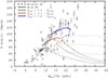 |
Fig. 2. Projected surface rotation velocity, Vsin(i), as a function of the near-core rotation velocity, Ωnc. The lines represent our simulations. The line types and colours have the same meanings as in Fig. 1, with the addition of a simulation where the initial rotation velocity is Vini = 0.3 ⋅ Vcrit (red). Colours are used only for the evolutionary stages in which the buoyancy radius remains within the range P0 = 4092 ± 575 s, which is consistent with the plotted observational data from Li et al. (2020). The surface velocities of our models have been multiplied by π/4 in order to take the unknown distribution of the inclination into consideration. |
At the end of the MS, the contraction of the core and expansion of the envelope can be observed with the lines evolving rapidly to the right, indicating that the BC instability does not seem to be strong enough to counteract the creation of differential rotation via this structural change, due to the large increase in the Brunt-Vaïsälä frequency. To illustrate this, we show in Fig. 3 the evolution of the near-core to surface rotation velocity ratios, as a function of the mixed mode density (𝒩), along with the observational data provided by Li et al. (2024). This illustrates an overestimation of the differential rotation in evolved stages both when rotation is treated without BC and when the BC instability is taken into consideration for the transport of AM. While providing an interesting physical explanation for the internal rotation of MS stars, AM transport through the BC instability is thus found to be insufficient to reproduce the low degree of radial differential rotation observed in the more evolved red giant stars.
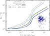 |
Fig. 3. Evolution of the ratio between the near-core and surface rotation velocities, as a function of the mixed mode density (𝒩). The observational data points are measurements of red giant stars from Li et al. (2024). The simulations are also shown; the line colours and styles have the same meanings as in Fig. 1. |
4. Conclusion
The quest for new physical processes able to explain the efficient coupling observed between stellar core and envelope rotation rates is still ongoing. In this Letter we have presented simulations made with GENEC in which an additional AM transport process based on the BC instability is implemented. Assuming solid-body rotation on the ZAMS, our simulations show that this instability is able to counteract the creation of radial differential rotation during the MS. The comparison of our simulations with the observations of near-core and projected surface velocities of γ Doradus stars available in the literature shows that AM transport by the BC instability enables the model to correctly account for the internal rotation of intermediate-mass stars on the MS. However, the BC instability is not able to explain the evolution of the internal rotation during the more advanced stages of the evolution, as shown by our comparison with the observations available for red giants.
Acknowledgments
MM, PE and CR acknowledge support from the FNS grant no 219745 (Asteroseismology of transport processes for the evolution of stars and planets). LS acknowledges support from the FNS grant no 212143 (Unique insight into binary stars and their close environment).
References
- Aerts, C., Van Reeth, T., Mombarg, J. S. G., & Hey, D. 2025, A&A, 695, A214 [NASA ADS] [CrossRef] [EDP Sciences] [Google Scholar]
- Beck, P. G., Montalban, J., Kallinger, T., et al. 2012, Nature, 481, 55 [Google Scholar]
- Belkacem, K., Marques, J. P., Goupil, M. J., et al. 2015, A&A, 579, A31 [NASA ADS] [CrossRef] [EDP Sciences] [Google Scholar]
- Bordadágua, B., Ahlborn, F., Coppée, Q., et al. 2025, A&A, 699, A310 [NASA ADS] [CrossRef] [EDP Sciences] [Google Scholar]
- Cantiello, M., Mankovich, C., Bildsten, L., Christensen-Dalsgaard, J., & Paxton, B. 2014, ApJ, 788, 93 [Google Scholar]
- Ceillier, T., Eggenberger, P., García, R. A., & Mathis, S. 2013, A&A, 555, A54 [NASA ADS] [CrossRef] [EDP Sciences] [Google Scholar]
- Deheuvels, S., García, R. A., Chaplin, W. J., et al. 2012, ApJ, 756, 19 [Google Scholar]
- Deheuvels, S., Doğan, G., Goupil, M. J., et al. 2014, A&A, 564, A27 [NASA ADS] [CrossRef] [EDP Sciences] [Google Scholar]
- Deheuvels, S., Ballot, J., Beck, P. G., et al. 2015, A&A, 580, A96 [NASA ADS] [CrossRef] [EDP Sciences] [Google Scholar]
- Deheuvels, S., Ouazzani, R. M., & Basu, S. 2017, A&A, 605, A75 [NASA ADS] [CrossRef] [EDP Sciences] [Google Scholar]
- Deheuvels, S., Ballot, J., Eggenberger, P., et al. 2020, A&A, 641, A117 [EDP Sciences] [Google Scholar]
- den Hartogh, J. W., Eggenberger, P., & Hirschi, R. 2019, A&A, 622, A187 [NASA ADS] [CrossRef] [EDP Sciences] [Google Scholar]
- den Hartogh, J. W., Eggenberger, P., & Deheuvels, S. 2020, A&A, 634, L16 [NASA ADS] [CrossRef] [EDP Sciences] [Google Scholar]
- Dhanpal, S., Benomar, O., Hanasoge, S., & Fuller, J. 2025, ApJ, 988, 224 [Google Scholar]
- Di Mauro, M. P., Ventura, R., Cardini, D., et al. 2016, ApJ, 817, 65 [NASA ADS] [CrossRef] [Google Scholar]
- Eggenberger, P., Maeder, A., & Meynet, G. 2005, A&A, 440, L9 [NASA ADS] [CrossRef] [EDP Sciences] [Google Scholar]
- Eggenberger, P., Meynet, G., Maeder, A., et al. 2008, Ap&SS, 316, 43 [Google Scholar]
- Eggenberger, P., Montalbán, J., & Miglio, A. 2012, A&A, 544, L4 [NASA ADS] [CrossRef] [EDP Sciences] [Google Scholar]
- Eggenberger, P., Buldgen, G., & Salmon, S. J. A. J. 2019a, A&A, 626, L1 [NASA ADS] [CrossRef] [EDP Sciences] [Google Scholar]
- Eggenberger, P., den Hartogh, J. W., Buldgen, G., et al. 2019b, A&A, 631, L6 [NASA ADS] [CrossRef] [EDP Sciences] [Google Scholar]
- Eggenberger, P., Buldgen, G., Salmon, S. J. A. J., et al. 2022a, Nat. Astron., 6, 788 [NASA ADS] [CrossRef] [Google Scholar]
- Eggenberger, P., Moyano, F. D., & den Hartogh, J. W. 2022b, A&A, 664, L16 [NASA ADS] [CrossRef] [EDP Sciences] [Google Scholar]
- Fujimoto, M. Y. 1987, A&A, 176, 53 [NASA ADS] [Google Scholar]
- Fujimoto, M. Y. 1988, A&A, 198, 163 [NASA ADS] [Google Scholar]
- Fujimoto, M. Y. 1993, ApJ, 419, 768 [Google Scholar]
- Fuller, J., Lecoanet, D., Cantiello, M., & Brown, B. 2014, ApJ, 796, 17 [Google Scholar]
- Fuller, J., Piro, A. L., & Jermyn, A. S. 2019, MNRAS, 485, 3661 [NASA ADS] [Google Scholar]
- Gebruers, S., Straumit, I., Tkachenko, A., et al. 2021, A&A, 650, A151 [NASA ADS] [CrossRef] [EDP Sciences] [Google Scholar]
- Gehan, C., Mosser, B., Michel, E., Samadi, R., & Kallinger, T. 2018, A&A, 616, A24 [NASA ADS] [CrossRef] [EDP Sciences] [Google Scholar]
- Gray, D. F. 1988, Lectures on Spectral-line Analysis: F, G, and K Stars (Arva: Ontario Gray) [Google Scholar]
- Li, G., Van Reeth, T., Bedding, T. R., et al. 2020, MNRAS, 491, 3586 [Google Scholar]
- Li, G., Deheuvels, S., & Ballot, J. 2024, A&A, 688, A184 [NASA ADS] [CrossRef] [EDP Sciences] [Google Scholar]
- Maeder, A. 1997, A&A, 321, 134 [NASA ADS] [Google Scholar]
- Marques, J. P., Goupil, M. J., Lebreton, Y., et al. 2013, A&A, 549, A74 [NASA ADS] [CrossRef] [EDP Sciences] [Google Scholar]
- Mombarg, J. S. G. 2023, A&A, 677, A63 [NASA ADS] [CrossRef] [EDP Sciences] [Google Scholar]
- Mosser, B., Goupil, M. J., Belkacem, K., et al. 2012, A&A, 548, A10 [NASA ADS] [CrossRef] [EDP Sciences] [Google Scholar]
- Moyano, F. D., Eggenberger, P., Salmon, S. J. A. J., Mombarg, J. S. G., & Ekström, S. 2023, A&A, 677, A6 [NASA ADS] [CrossRef] [EDP Sciences] [Google Scholar]
- Moyano, F. D., Eggenberger, P., & Salmon, S. J. A. J. 2024, A&A, 681, L16 [NASA ADS] [CrossRef] [EDP Sciences] [Google Scholar]
- Ouazzani, R.-M., Salmon, S. J. A. J., Antoci, V., et al. 2017, MNRAS, 465, 2294 [Google Scholar]
- Ouazzani, R. M., Marques, J. P., Goupil, M. J., et al. 2019, A&A, 626, A121 [NASA ADS] [CrossRef] [EDP Sciences] [Google Scholar]
- Pinçon, C., Belkacem, K., Goupil, M. J., & Marques, J. P. 2017, A&A, 605, A31 [NASA ADS] [CrossRef] [EDP Sciences] [Google Scholar]
- Saio, H., Takata, M., Lee, U., Li, G., & Van Reeth, T. 2021, MNRAS, 502, 5856 [Google Scholar]
- Spruit, H. C. 2002, A&A, 381, 923 [CrossRef] [EDP Sciences] [Google Scholar]
- Tayar, J., Beck, P. G., Pinsonneault, M. H., García, R. A., & Mathur, S. 2019, ApJ, 887, 203 [NASA ADS] [CrossRef] [Google Scholar]
- Tayler, R. J. 1973, MNRAS, 161, 365 [CrossRef] [Google Scholar]
- Triana, S. A., Corsaro, E., De Ridder, J., et al. 2017, A&A, 602, A62 [NASA ADS] [CrossRef] [EDP Sciences] [Google Scholar]
- Van Reeth, T., Tkachenko, A., & Aerts, C. 2016, A&A, 593, A120 [NASA ADS] [CrossRef] [EDP Sciences] [Google Scholar]
- Van Reeth, T., Mombarg, J. S. G., Mathis, S., et al. 2018, A&A, 618, A24 [NASA ADS] [EDP Sciences] [Google Scholar]
- Zahn, J. P. 1992, A&A, 265, 115 [NASA ADS] [Google Scholar]
Appendix A: Impact of the baroclinic instability on the internal AM transport
To discuss the relative importance of AM transport through meridional currents and the shear instability, we define an approximate characteristic diffusion coefficient DMC = |r ⋅ U| for the meridional circulation (even if the advective nature of this transport is fully accounted for in the simulations); this allows us to easily compare the efficiency of these two transport mechanisms. We first illustrate in Fig. A.1 the case of models without BC. Figure A.1 shows these two diffusion coefficients for the shear instability and the meridional circulation in the middle of the MS (Xc ∼ 0.35). This illustrates that AM transport is mostly dominated by meridional circulation in models without BC, with only a contribution from the shear instability in the outer layers.
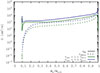 |
Fig. A.1. Diffusion coefficients for the shear Dshear (dashed lines) and for the meridional circulation DMC (solid lines) for simulations without BC. |
We then compare the efficiency of the different AM transport processes for models accounting for the BC instability. We first present in Fig. A.2 the Richardson numbers ℛi and ℛiBC for a model with BC, and an initial rotation velocity of Vini = 0.2 ⋅ Vcrit for different evolutionary stages on the MS, as well as one red giant profile. Figure A.2 shows that the hypothesis of ℛi ≫ 1 used for the derivation of the AM transport associated to the BC instability is well verified at every location in the radiative interior of these intermediate mass stars, from the MS to the red giant phase. Moreover, the Richardson number ℛi is found to be always larger than the critical Richardson number for the BC instability ℛiBC, which indicates that the BC instability stays in the second regime in Eq. (2).
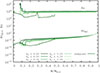 |
Fig. A.2. Richardson numbers profiles ℛi and ℛiBC as a function of the normalized mass for a model with BC, and an initial rotation velocity of Vini = 0.2 ⋅ Vcrit. These profiles are shown in the radiative zone only for different evolutionary stages on the MS expressed as a function of the central hydrogen mass fraction, Xc. The red giant model is characterized by a surface gravity of log(g) = 3.5. |
Figures A.3 and A.4 present the diffusion coefficient related to the BC instability DBC in addition to Dshear and DMC for models with BC in the middle of the MS (Xc ∼ 0.35). The BC instability tends to dominate in nearly all the internal layers of the star, while at the centre AM transport is dominated by the meridional currents. Comparing Fig. A.3 and A.4 with Fig. A.1, it is interesting to note that the strength of the secular shear instability is smaller than in the simulations without BC. This is explained by the fact that BC instability tends to decrease the gradient of rotation. The secular shear instability is thus reduced as it evolves proportionally to dΩ/dr. Moreover, the meridional circulation appears to be stronger in simulations taking into consideration the BC instability. Finally, we note that the diffusion coefficient for the BC instability is higher for the simulation with an initial rotation velocity of Vini = 0.4 ⋅ Vcrit. The efficiency of this additional transport process leads to flatter rotation profiles for models with BC, as shown in Fig. A.5 for two different evolutionary stages.
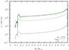 |
Fig. A.3. Diffusion coefficients for the BC instability (DBC; solid line), the shear instability (Dshear; dashed line), and the meridional circulation (DMC; dotted lines) for a model with BC and an initial rotation velocity of Vini = 0.2 ⋅ Vcrit in the middle of the MS (Xc ∼ 0.35). |
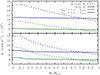 |
Fig. A.5. Angular rotation velocity profiles as a function of the normalized mass at the middle of the MS (Xc ∼ 0.35, top panel) and near the end of the MS (Xc ∼ 0.1, bottom panel). The colour codes and line styles have the same meaning as in Fig. 1. |
Appendix B: Effects of the modelling of the baroclinic instability
We discuss here the impact of the exact modelling of the AM transport through the BC instability on the conclusions obtained in the present study. Following Fujimoto (1993), we compute new models with a much lower value of the parameter αBC of 0.001 instead of 1; this corresponds to a significant decrease in the transport efficiency through the BC instability compared to the models shown previously. The evolution of the ratio of core to surface rotation rates is shown in Fig. B.1 for these models. As expected, the decrease in αBC leads to an increase in the radial differential rotation. However, despite the significant change in αBC, the BC instability still impacts the internal rotation of the models by reducing the degree of radial differential rotation compared to the one predicted by models without BC.
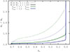 |
Fig. B.1. Same as Fig. 1 but for models computed for two different values of the BC parameter αBC. Solid and dotted lines correspond to models with αBC of 1 and 0.001, respectively. |
We finally compare the predictions of these rotating models computed with αBC = 0.001 to the observational constraints on the core and surface rotation rates available for γ-Doradus stars. This comparison is shown in Fig. B.2 together with the results previously obtained by adopting αBC = 1. Baroclinic models with αBC = 0.001 (dotted lines in Fig. B.2) are then found to exhibit a very similar evolution compared to models with αBC = 1 (solid lines in Fig. B.2). Despite the significant decrease in αBC, one sees that these baroclinic models are still able to correctly account for these observations, which cannot be correctly reproduced by models without BC (see dashed lines in Fig. 2). We thus find that our global conclusions about the impact of the BC instability on the rotational properties of γ-Doradus stars do not depend on the exact value adopted for the parameter αBC entering into the modelling of this instability.
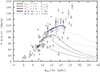 |
Fig. B.2. Same as Fig. 2 but for models computed for two different values of the BC parameter αBC. Solid and dotted lines correspond to models with αBC of 1 and 0.001, respectively. |
Appendix C: Impact of the inclination angle
In Fig. 2 the surface rotation velocities of our models have been multiplied by π/4 in order to account for the unknown inclination angle i. This factor is obtained from the mean value of sin(i) by assuming an isotropic distribution of i with a probability given by P(i)di = 2π sin(i) di, and thus ⟨sin(i)⟩ = ∫P(i)sin(i)di/∫P(i)di = π/4 (see Gray 1988). This choice of an isotropic distribution assumes that no specific value for the inclination i should be preferred. However, one could also argue that high inclination angles should be preferred, for instance due to observed oscillation amplitudes that tend to be larger for higher inclination angles (see e.g. Van Reeth et al. 2018). In this case, the correction factor will be between π/4 and the extreme case of sin(π/2) = 1. We thus present in Fig. C.1 the same figure as Fig. 2 but considering a factor of 1 instead of π/4. By doing so, the lines are slightly shifted upwards, and now correspond to the upper limit on the projected surface rotation velocity. Indeed, the theoretical predictions now assume that the stars are only seen with an inclination angle of i = π/2, i.e. Vsin(i) corresponds exactly to the surface equatorial rotation velocity. Figure C.1 shows that the vast majority of the observed Vsin(i) cannot be reproduced by models without BC, since they are located above the maximal values predicted by these models (dashed lines in Fig. C.1); these results are in good agreement with previous studies of Ouazzani et al. (2019) and Moyano et al. (2023). In contrary, for models with BC (solid lines in Fig. C.1), the vast majority of the observed Vsin(i) are located below the maximal values predicted by these models. This shows that models with BC have no difficulties to reproduce those points, recalling that lower values of theoretical Vsin(i) can be obtained by assuming an inclination angle i lower than π/2.
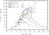 |
Fig. C.1. Same as Fig. 2 but without the multiplying factor π/4 for the surface velocities of the models, which was previously used to account for the unknown inclination angle. In this case, the lines correspond to an upper limit on the projected surface rotation velocity. |
All Figures
|
Fig. 1. Evolution of the core-to-surface rotation rates as a function of the central hydrogen mass fraction for a 1.5 M⊙ star at solar metallicity. Dashed (solid) lines show the models without (with) the BC instability. The colours differentiate models starting with an initial rotation velocity on the ZAMS of Vini = 0.2 ⋅ Vcrit (green) and Vini = 0.4 ⋅ Vcrit (blue). The vertical lines indicate the evolutionary stages where the rotation profiles are shown in Fig. A.5. |
| In the text | |
|
Fig. 2. Projected surface rotation velocity, Vsin(i), as a function of the near-core rotation velocity, Ωnc. The lines represent our simulations. The line types and colours have the same meanings as in Fig. 1, with the addition of a simulation where the initial rotation velocity is Vini = 0.3 ⋅ Vcrit (red). Colours are used only for the evolutionary stages in which the buoyancy radius remains within the range P0 = 4092 ± 575 s, which is consistent with the plotted observational data from Li et al. (2020). The surface velocities of our models have been multiplied by π/4 in order to take the unknown distribution of the inclination into consideration. |
| In the text | |
|
Fig. 3. Evolution of the ratio between the near-core and surface rotation velocities, as a function of the mixed mode density (𝒩). The observational data points are measurements of red giant stars from Li et al. (2024). The simulations are also shown; the line colours and styles have the same meanings as in Fig. 1. |
| In the text | |
|
Fig. A.1. Diffusion coefficients for the shear Dshear (dashed lines) and for the meridional circulation DMC (solid lines) for simulations without BC. |
| In the text | |
|
Fig. A.2. Richardson numbers profiles ℛi and ℛiBC as a function of the normalized mass for a model with BC, and an initial rotation velocity of Vini = 0.2 ⋅ Vcrit. These profiles are shown in the radiative zone only for different evolutionary stages on the MS expressed as a function of the central hydrogen mass fraction, Xc. The red giant model is characterized by a surface gravity of log(g) = 3.5. |
| In the text | |
|
Fig. A.3. Diffusion coefficients for the BC instability (DBC; solid line), the shear instability (Dshear; dashed line), and the meridional circulation (DMC; dotted lines) for a model with BC and an initial rotation velocity of Vini = 0.2 ⋅ Vcrit in the middle of the MS (Xc ∼ 0.35). |
| In the text | |
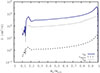 |
Fig. A.4. Same as Fig. A.4 but for a model with an initial rotation velocity of Vini = 0.4 ⋅ Vcrit. |
| In the text | |
|
Fig. A.5. Angular rotation velocity profiles as a function of the normalized mass at the middle of the MS (Xc ∼ 0.35, top panel) and near the end of the MS (Xc ∼ 0.1, bottom panel). The colour codes and line styles have the same meaning as in Fig. 1. |
| In the text | |
|
Fig. B.1. Same as Fig. 1 but for models computed for two different values of the BC parameter αBC. Solid and dotted lines correspond to models with αBC of 1 and 0.001, respectively. |
| In the text | |
|
Fig. B.2. Same as Fig. 2 but for models computed for two different values of the BC parameter αBC. Solid and dotted lines correspond to models with αBC of 1 and 0.001, respectively. |
| In the text | |
|
Fig. C.1. Same as Fig. 2 but without the multiplying factor π/4 for the surface velocities of the models, which was previously used to account for the unknown inclination angle. In this case, the lines correspond to an upper limit on the projected surface rotation velocity. |
| In the text | |
Current usage metrics show cumulative count of Article Views (full-text article views including HTML views, PDF and ePub downloads, according to the available data) and Abstracts Views on Vision4Press platform.
Data correspond to usage on the plateform after 2015. The current usage metrics is available 48-96 hours after online publication and is updated daily on week days.
Initial download of the metrics may take a while.