| Issue |
A&A
Volume 684, April 2024
|
|
|---|---|---|
| Article Number | A169 | |
| Number of page(s) | 22 | |
| Section | Stellar structure and evolution | |
| DOI | https://doi.org/10.1051/0004-6361/202346979 | |
| Published online | 19 April 2024 | |
Impact of different approaches to computing rotating stellar models
I. The case of solar metallicity
1
Département d’Astronomie, Université de Genève, Chemin Pegasi 51, 1290 Versoix, Switzerland
e-mail: This email address is being protected from spambots. You need JavaScript enabled to view it.
2
Institut d’Astronomie et d’Astrophysique, Université Libre de Bruxelles, Campus de la Plaine, CP226 Bruxelles, Belgium
Received:
23
May
2023
Accepted:
20
December
2023
Abstract
Context. The physics of stellar rotation plays a crucial role in the evolution of stars, in their final fates, and for the properties of compact remnants.
Aims. Diverse approaches have been adopted to incorporate the effects of rotation in stellar evolution models. This study seeks to explore the consequences that these various prescriptions for rotation have for the essential outputs of massive star models.
Methods. We computed a grid of 15 and 60 M⊙ stellar evolution models with the Geneva Stellar Evolution Code that accounted for both hydrodynamical and magnetic instabilities induced by rotation.
Results. In the 15 and 60 M⊙ models, the choice of the vertical and horizontal diffusion coefficients for the nonmagnetic models strongly impacts the evolution of the chemical structure, but has a weak impact on the angular momentum transport and the rotational velocity of the core. In the 15 M⊙ models, the choice of the diffusion coefficient impacts the convective core size during the core H-burning phase, regardless of whether the model begins core He-burning as a blue or red supergiant and regardless of the core mass at the end of He-burning. In the 60 M⊙ models, the evolution is dominated by mass loss and is less strongly affected by the choice of the diffusion coefficient. In the magnetic models, magnetic instability dominates the angular momentum transport, and these models are found to be less strongly mixed than their rotating nonmagnetic counterparts.
Conclusions. Stellar models with the same initial mass, chemical composition, and rotation may exhibit diverse characteristics depending on the physics applied. By conducting thorough comparisons with observational features, we can ascertain which method(s) produce the most accurate results in different cases.
Key words: stars: evolution / stars: massive / stars: rotation
© The Authors 2024
 Open Access article, published by EDP Sciences, under the terms of the Creative Commons Attribution License (https://creativecommons.org/licenses/by/4.0), which permits unrestricted use, distribution, and reproduction in any medium, provided the original work is properly cited.
This article is published in open access under the Subscribe to Open model. This email address is being protected from spambots. You need JavaScript enabled to view it. to support open access publication.
1. Introduction
The impact of rotation on the evolution of stars has been the subject of extensive research (e.g. Maeder & Meynet 2012, and references therein). The mechanical equilibrium of stars is altered by rotation, resulting in deformations (Kippenhahn & Thomas 1970; Meynet & Maeder 1997) and triggering instabilities that transport chemical elements and angular momentum (see Endal & Sofia 1981; Zahn 1992; Maeder & Zahn 1998; Spruit 2002, for the equations of transport corresponding to various instabilities as they can be implemented in 1D stellar evolution models). Rotation influences mass loss due to line-driven stellar winds (Maeder 1999, 2002; Heger et al. 2000; Müller & Vink 2014; Bogovalov et al. 2021), and it can lead to mechanical mass loss when the surface velocities reach the critical value at which centrifugal acceleration balances gravity (see, e.g., Krtička et al. 2011; Georgy et al. 2013a).
The inclusion of rotation in a star can result in a very different track in the Hertzsprung-Russell (HR) diagram. On the modeling side, this phenomenon is well illustrated by the case of chemically homogeneous evolution, which is triggered by efficient rotational mixing (Maeder 1987; Mandel & de Mink 2016; de Mink & Mandel 2016; Song et al. 2016). The mass limits between different evolutionary scenarios are different depending on the initial rotation or initial angular momentum content at the zero-age main-sequence (ZAMS). For instance, the lower mass limits for single stars evolving into the Wolf-Rayet phase (Meynet & Maeder 2005) or undergoing a pair instability supernova depend on rotation (Chatzopoulos & Wheeler 2012; Marchant & Moriya 2020). Nucleosynthesis in massive stars can be significantly influenced by their rotation, especially for certain isotopes. Notable examples include 26Al at solar metallicity (Palacios et al. 2005; Brinkman et al. 2021, 2023; Martinet et al. 2022), 14N at very low metallicity (Meynet & Maeder 2002), and the s-process (Pignatari et al. 2008; Frischknecht et al. 2016; Choplin et al. 2018; Limongi & Chieffi 2018; Banerjee et al. 2019). The pre-supernova stage is greatly affected by rotation, where it influences the core collapse and the properties of the stellar remnant (Hirschi et al. 2004, 2005a; Limongi & Chieffi 2018; Fields 2022). Rotation also appears to be a key ingredient when exploring many topical astrophysical questions, such as the nature of the progenitors of the long gamma-ray bursts (Hirschi et al. 2005b; Yoon et al. 2006), the origin of primary nitrogen in the early Universe (Chiappini et al. 2006), and the spin and mass limits of stellar black holes and neutron stars (Heger et al. 2005; Fuller & Ma 2019; Griffiths et al. 2022; Fuller & Lu 2022).
In the past decades, many stellar evolution models for single and binary stars that accounted for the effects of rotation have been published (see e.g. Brott et al. 2011; Ekström et al. 2012; Choi et al. 2016; Limongi & Chieffi 2018; Renzo & Götberg 2021; Nguyen et al. 2022; Pauli et al. 2022; Renzo et al. 2023). These models are based on different approaches to incorporating the effects of rotation, and in particular, on the transport of the angular momentum and of the chemical species in the interior. As a result, models with a given initial mass, rotation, and composition may produce significantly different outputs. The differences arise from the nature of the physical processes included and from the way a given physical process is numerically implemented in the stellar evolution code.
Rotating models for massive stars can be roughly classified into two main families: nonmagnetic and magnetic rotating models. In this context, the term magnetic does not refer to the existence of a surface magnetic field here (Meynet et al. 2011; Keszthelyi et al. 2020). Instead, it refers to the action of a dynamo based on the magnetic Tayler instability (Spruit 2002), hereafter called the Tayler–Spruit dynamo theory, or of another magnetic instability operating in the interior of a star. Examples of grids of nonmagnetically rotating models are those of Ekström et al. (2012), Choi et al. (2016), Limongi & Chieffi (2018), and Nguyen et al. (2022). Examples of magnetic models can be found in Heger et al. (2005) and Brott et al. (2011).
A first discussion of the impact of different prescriptions in the Geneva Stellar Evolution Code (GENEC) for rotation was presented in Meynet et al. (2013). In this work, we present a more extensive and detailed analysis. We study the outputs for nonmagnetic and magnetic massive star models with masses of 15 and 60 M⊙ at solar metallicity obtained using different implementations for the various diffusion coefficients entering the theory (see Sect. 3). More precisely, we study the implications of these different choices on the following model outputs:
-
The evolutionary tracks and lifetimes during the MS phase and the core helium-burning phase.
-
The changes in the surface composition and velocity.
-
The timescale for the crossing of the HR gap and the impact on the lifetimes of blue and red supergiants.
-
The evolution of the internal angular velocity.
-
The properties of the stellar cores at the end of the core He-burning phase.
We also discuss the impact of the different prescriptions on the boron depletion at the surface of massive rotating stars at the very beginning of the core hydrogen-burning phase. The depletion of boron is an indication of shallow mixing that is probably associated with mixing processes within the star and probably does not result from mass transfer in a close binary system (see the discussion in Fliegner et al. 1996). As a result, this feature seems to probe the physics of the mixing in a rather clean way (Proffitt et al. 1999, 2016; Proffitt & Quigley 2001; Venn et al. 2002; Mendel et al. 2006; Frischknecht et al. 2010). We discuss the effects of different prescriptions on the case of a 60 M⊙ model at solar metallicity whose evolution is strongly impacted by mass loss through stellar winds. Finally, we also compare this with magnetic models, which point was not addressed in Meynet et al. (2013). In an accompanying paper, we will study the impacts of these different implementations at very low metallicity (Nandal et al., in prep.).
We begin the paper with a brief discussion of the transport equations in rotating models in Sect. 2 and the implementation of these equations in the stellar models in Sect. 3. In Sects. 4 and 5, we discuss the results for the 15 and 60 M⊙ and models that account for hydrodynamical instabilities induced by rotation. The magnetic models for both the 15 and 60 M⊙ models are presented in Sect. 6. In Sect. 7, we present our conclusions.
2. The transport equations
All the models considered in this work are assumed to have nearly uniform rotation along an isobar (shellular rotating models). The homogenization of the horizontal angular velocity in a star is achieved by a strong isobaric or horizontal turbulence, which also causes other physical quantities such as temperature and density to become uniform at a given level within the star (see the discussion in Zahn 1992). We assume this to be true because the restoring force (gravity) prevents strong turbulence in the vertical direction.
The transport of chemical species in the context of the shellular theory of rotation is governed by a purely diffusive equation (Chaboyer & Zahn 1992) that is written as
 (1)
(1)
where Xi is the abundance in mass fraction of isotope i, and Dchem is the appropriate diffusion coefficient for the transport of the chemical elements. Equation (1) only describes the change in the abundance of an isotope at a given position due to the rotational diffusion. In the stellar models, two other processes, convection and nuclear reactions, are accounted for. The other symbols ρ, r, Mr are the density, the radius, and the Lagrangian mass coordinate.
In a differentially rotating star, the evolution of the angular velocity Ω has to be followed at each level r, so that a full description of Ω(r, t) is available. In the case of shellular rotation (Zahn 1992), the equation describing the transport of angular momentum in Lagrangian form is
 (2)
(2)
U2 is the radial component of the velocity of the meridional circulation along the vertical direction, that is, U(r, θ) = U2(r)P2(cos θ), where P2 is the Legendre polynomial of second order, and Dang is the appropriate diffusion coefficient for the transport of the angular momentum.
As explained in more detailed below, we discuss the outputs of numerical experiments by comparing models that have the same set of assumptions and differ in the algorithmic and numerical treatment of one particular aspect (rotation).
3. Diffusive/viscosity coefficients
In this section, we discuss the expressions for the diffusive coefficients entering Eqs. (1) and (2). In the equation for the transport of the chemical species for nonmagnetic models, Dchem is equal to the sum of two terms: Dshear and Deff. Dshear corresponds to the transport of chemicals and angular momentum by the shear instability, while Deff describes the transport of the chemical elements due to the combined action of meridional currents and horizontal turbulence (Chaboyer & Zahn 1992). In the equation for the transport of the angular momentum, Dang is equal to Dshear for the nonmagnetic models.
In magnetic models, Dchem is equal to the sum of three terms: Dshear, Deff, and the direct transport of chemicals by the Tayler–Spruit dynamo ηTS. In the equation for the transport of angular momentum, Dang is the sum of two terms: Dshear, and the viscosity associated with angular momentum by the Tayler–Spruit dynamo νTS. In magnetic models, the transport of angular momentum by the meridional currents is much smaller that the transport due to the magnetic coupling, and therefore, only the transport by magnetic coupling is considered. The transport of chemical species is dominated by Deff, and therefore, ηTS is neglected.
3.1. The vertical shear diffusion, Dshear
The vertical shear diffusion coefficient Dshear accounts for the transport of chemical species and angular momentum in the radial direction, which is caused by turbulence triggered by differential rotation in the vertical direction. For this coefficient, two different expressions are used in the literature, Maeder (1997) and Talon & Zahn (1997). Taken in the limit where the radiative diffusive coefficient K is extremely large and the shear instability has a negligible impact on the energy transport, the expression of Dshear from Maeder (1997) is
![Mathematical equation: $$ \begin{aligned} D_{\rm shear} = f_{\rm en} \frac{H_{\rm P}}{g\delta }\frac{K}{\left[\frac{\varphi }{\delta }\nabla _\mu + \left(\nabla _{\rm ad} - \nabla _{\rm rad}\right)\right]} \left(\frac{9\pi }{32}\ \Omega \ \frac{\mathrm{d} \ln \Omega }{\mathrm{d} \ln r}\right)^2, \end{aligned} $$](/articles/aa/full_html/2024/04/aa46979-23/aa46979-23-eq3.gif) (3)
(3)
where fen indicates the fraction of the available energy that can be used for the mixing. In our models, we used fen = 1, HP, the pressure scale height, g, the gravity, 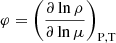 ,
,  is the radiative diffusion coefficient, and
 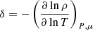 ,
,  ,
,  ,
,  . The expression of Dshear from Talon & Zahn (1997) is
![Mathematical equation: $$ \begin{aligned} D_{\rm shear} = f_{\rm en} \frac{H_{\rm P}}{g\delta }\frac{\left(K+D_{\rm h}\right)}{\left[\frac{\varphi }{\delta }\nabla _\mu \left(1+\frac{K}{D_{\rm h}}\right) + \left(\nabla _{\rm ad} - \nabla _{\rm rad} \right)\right]} \left(\frac{9\pi }{32}\ \Omega \ \frac{\mathrm{d} \ln \Omega }{\mathrm{d} \ln r} \right)^2, \end{aligned} $$](/articles/aa/full_html/2024/04/aa46979-23/aa46979-23-eq10.gif) (4)
(4)
where Dh is the horizontal turbulence diffusion coefficient.
3.2. The horizontal turbulence, Dh
The strong horizontal turbulence is triggered by shear along an isobar. Differential rotation on an isobar can result from the action of meridional currents. Various expressions have been proposed by different authors. We recall them below. They contain parameters whose values were taken as proposed in the original publications. We refer to these publications for the justifications of these choices.
Three different expressions for Dh are used in the literature. Zahn (1992) expressed it as
 (5)
(5)
where 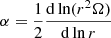 , and V(r) is the horizontal component of the meridional circulation velocity. The original formula by Zahn (1992) is multiplied by
  , but ch is then taken equal to 1. Maeder (2003) expressed the equation as
 (6)
(6)
with α as in Eq. (5), and A = 0.002. Mathis et al. (2004) expressed Dh as
 (7)
(7)
with α as in Eq. (5) and β = 1.5 × 10⁻⁶. In all the above expressions, Ω is the latitude-averaged value of the angular velocity along an isobar. The variations in the angular velocity with respect to the latitude on a given isobar are expected to very small as a result of the action of the strong horizontal turbulence.
3.3. The effective diffusion, Deff
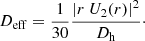
All prescriptions used the same effective mixing coefficient, Deff, for the chemical species given by Chaboyer & Zahn (1992) and Zahn (1992),
 (8)
(8)
As briefly recalled in Appendix A, the factor 1/30 results from an integration and is not a parameter whose value can be chosen.
Although the expression of U shows a dependence on Dh, this dependence remains small as long as Dh is much smaller than K. This is the case in all of our models. As indicated by Eq. (8), Dh is inversely proportional to Deff. The horizontal turbulence limits any vertical movement, similar to how a strong horizontal wind would bend the trajectory of smoke from a chimney.
3.4. The magnetic diffusivity, ηTS
The magnetic models used in this paper are based on the Tayler–Spruit calibrated dynamo described in Eggenberger et al. (2022a). This approach builds upon the theory of the Tayler–Spruit dynamo (Spruit 2002), and was calibrated in order to fit the internal distributions of angular velocity in subgiants and red giant stars as deduced from asteroseismic analysis.
The transport of chemical elements by magnetic instability is described by a magnetic diffusion coefficient, ηTS. The magnetic diffusion coefficient is in absence of any instability the ohmic diffusion coefficient as given in Spitzer (1956). When the condition for magnetic instability is realized, the values of ηTS and of the Alfvén frequency can be obtained from two conditions that are valid at the limit at which the instability is triggered (see the discussion in Eggenberger et al. 2022a).
This magnetic diffusion is not very strong compared to the transport of chemical species by Deff. It is is neglected in our models. However, this quantity needs to be computed because it is used in the expression for the magnetic viscosity (see below).
3.5. The magnetic viscosity, νTS
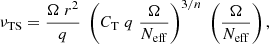
The transport of the angular momentum is described by the magnetic viscosity parameter νTS. The viscosity is then obtained using the general formula given by Eq. (8) of Eggenberger et al. (2022a),
 (9)
(9)
with n = 1, CT = 216 and 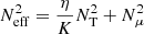 ,
, 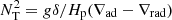 , and
, and  . The value of CT was chosen so that the models can reproduce the core rotation rates of red giants determined based on asteroseismology by Gehan et al. (2018). In the original version of the Tayler–Spruit dynamo CT = 1 (Spruit 2002). The version with CT = 216 has been called the calibrated Tayler–Spruit dynamo by Eggenberger et al. (2022a). Tayler–Spruit dynamo provides an evolution of the core rotation similar to that given by the Fuller et al. (2019) approach. This magnetic angular momentum transport is only accounted for when the shear parameter
  exceeds a minimum value qmin given by Eq. (12) of Eggenberger et al. (2022a),
 (10)
(10)
3.6. Parameters of the stellar models
The additional parameters of the stellar models were chosen as described in Ekström et al. (2012). In particular, the models were computed with a moderate step overshoot (αov = 0.1), used the same mass-loss rates, and did not account for surface magnetic fields. The convective zones rotated as solid bodies and were chemically homogeneous. More details of the models can be found in Appendix B.
We chose to focus on two initial masses that are representative of the evolution of massive stars. The first was a 15 M⊙ model that illustrates the case of single stars evolving into a red supergiant stage after the main sequence and exploding as a type IIP supernova at the end of their evolution. The second was the case of a single 60 M⊙ model evolving into a luminous blue variable phase after the main sequence and evolving into a Wolf-Rayet phase. This is representative of the upper mass range of single massive stars whose evolution at solar metallicity is mainly affected by mass loss. All the models were computed using the fully advective-diffusive approach (according to Eq. (2)) during the MS phase and using a purely diffusive approach during the core helium-burning phase.
We did not impose values to uncertain parameters involved in the expressions for the diffusion coefficients to enforce the model to reproduce a given observational features, as is commonly done when grids of rotating models are computed. Instead, we considered the same physical assumption for all the models to set the parameter fen in Dshear and otherwise, chose different values for the parameters A or β in the different expressions for Dh suggested by the original publications. To set fen, we assumed for all the models that the whole excess energy available in the differential rotation (shear energy) can be used to drive the transport, and the critical Richardson number was taken equal to one-fourth (for a detailed discussion of the physics of fen and Richardson, we refer to Appendices A and B, respectively). These two assumptions do not vary when we use different prescriptions because all of them are based on similar physics. In this way, we compared the impacts of different physical approaches without any fine-tuning to reproduce an observed feature. The outputs of the models are comparable, however, because they are based on common physical assumptions at a more fundamental level.
Table 1 lists all the models we discuss here. The first column lists the model label. The prescription we used is given in Col. 2: Ma97, TZ97 means that the expression for the shear diffusion is given by Maeder (1997) and Talon & Zahn (1997). Za92, Ma03, and MZ04 indicates that the expression of the horizontal diffusion coefficient is given by Zahn (1992), Maeder (2003), and Mathis et al. (2004). The time-averaged equatorial velocity during the MS phase is listed in Col. 3, the MS lifetime is listed in Col. 4, and the surface helium abundance in mass fraction at the end of the MS phase is listed in Col. 5. Column 6 presents the N/H ratio obtained at the surface at the end of the MS phase. This is normalized to the initial N/H value. The actual mass of the star at the end of the core H-burning phase is indicated in Col. 7. The core He-burning lifetime and the times of the core He-burning phase spent in the red (log Teff < 3.68), blue (log Teff > 3.87), and yellow part (3.68 < log Teff < 3.87) of the HR diagram are listed in Cols. 8–11 respectively. The ratio of the time spent in the blue to that spent in the red is shown in Col. 12. The mass fraction of helium at the surface is given in Col. 13 and the actual mass at the end of the core He-burning lifetime in Col. 14. The masses of the helium and carbon-oxygen cores () and the mass of the remnants are given in Cols. 15–17 and were obtained using the formulation from Maeder (1992). The masses of the helium and CO cores were obtained finding the first shell scanning the star from the surface to the interior, where the mass fraction of helium and the sum of the mass fraction of carbon and oxygen, respectively, is higher than 0.75). Model C* was computed using the same prescription as for model C, but it additionally includes the effects of magnetic fields as described in Sect. 3.4.
Some properties of the models.
Some differences between models of the same initial mass that were computed with different prescriptions for the rotational mixing are small in the sense that some change in the numerics (time or space resolution) can produce similar changes. They are also small in the sense that they cannot be distinguished in observations. This mainly concerns differences due to the different prescriptions of the HR track during the MS phase. While this needs to be recalled for our results, we would like to stress, however, that the techniques governing the choice of the time and space resolution (briefly described in Appendix B) were kept exactly the same for all the computations. This allowed thus to give a correct idea of the relative changes brought by the different prescriptions.
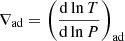
4. The results of nonmagnetic 15 M⊙ models
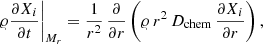
4.1. The diffusion coefficients
Figure 1 illustrates the variation in the diffusion coefficients with radius when the central mass fraction of hydrogen is 0.35. The qualitative features that are similar in all six models are listed below.
 |
Fig. 1. Internal profiles of K, the thermal diffusivity, Dconv, the convective diffusion coefficient, Dshear, the shear diffusion coefficient, Dh, the horizontal turbulence coefficient, and Deff, the effective diffusivity in 15 M⊙ models at solar metallicity. Each panel is labeled with a letter corresponding to the first column of Table 1. The profile is taken when the central mass fraction of hydrogen Xc = 0.35. |
– In the convective core, the diffusion coefficient is large enough to homogenize the chemical composition. Here, it is about 1012 cm2 s−1. The reason is the physics of convection and not the rotation.
– The thermal diffusion coefficient K increases outward and is well above the diffusion coefficients describing the rotational instabilities. Thus, the thermal diffusion timescale is much shorter than the timescales of the rotational instabilities, indicating that the rotational instabilities do not significantly contribute to the transport of energy.
– Dh serves as the primary rotational diffusion coefficient in most of the radiative region, and it is strong enough to achieve shellular rotation.
Rotational mixing can facilitate the transfer of an element from the core to the surface. During the MS phase, an element that is transported from the core to the surface passes through four zones. The first zone is the convective core, where the transport of the chemical species is very efficient. The second zone is located immediately above the core, and it is characterized by a gradient in the mean molecular weight. The chemical gradient arises because the nuclear timescale is shorter than the mixing timescale in the whole radiative envelope. The gradient is steeper in the layers directly surrounding the core, and it becomes smoother when progressing outward (see the middle panel of Fig. 2) because during the MS phase, the convective core decreases in mass. The outer portion of this zone is therefore representative of the initial impact of the nuclear reactions in the core. In regions with a steep μ-gradient, the vertical shear diffusion coefficient is strongly reduced by the μ-gradients, and the main diffusion coefficient for transporting the chemical species is Deff. The Deff is smaller when the value of Dh is higher. Thus, the choice of Dh has a significant impact on the way in which diffusion of the chemical species occurs in the second region. In the third zone,  is significantly larger than the difference ∇ad − ∇rad, the ratio Dshear(M97)/Dshear(TZ97) ∼ K/Dh. Since Dh is lower than K, we have Dshear(M97) > Dshear(TZ97). The mixing in this region therefore depends on the vertical shear diffusion coefficient. Finally, zone 4 covers all the outer layers above zone 3. Here, the mixing of the elements is also governed by Dshear, but the value of Dshear is the same, regardless of whether Maeder (1987) or Talon & Zahn (1997) is used. In zones without μ-gradients, Dshear(M97)/Dshear(TZ97) ∼ K/(K + Dh)∼1 because Dh is smaller than K.
 |
Fig. 2. Evolution of various physical parameters of the 15 M⊙ models. Left panel: evolutionary tracks during the MS phase in the Hertzsprung-Russell diagram of the 15 M⊙ at Z = 0.014 and with Vini/Vcrit = 0.4. The letters A to G correspond to the models described in Table 1. Center panel: variation in the mass fraction of hydrogen as a function of the Lagrangian mass coordinate when the central mass fraction of hydrogen is 0.35 (Xc = 0.35). Right panel: evolution of the angular velocity vs. the internal mass coordinate at Xc = 0.35 through hydrogen burning. |
4.1.1. The vertical shear diffusion coefficient Dshear
In the first two upper panels of Fig. 1, we compare the impact of transitioning from the expression of Maeder (1997) to that of Talon & Zahn (1997) for Dshear while keeping the same expression of Zahn (1992) for Dh. Even when the same expression for Dh is used, the profile of Dh inside the two models is not equivalent (see models A and B) because changing Dshear modifies the chemical structure of the model and hence its structure at a given evolutionary stage. The same is true for Deff. We note that when Dshear of Maeder (1997) is used, the zone in which Deff dominates is significantly smaller. This is due to the impact of the stronger value given by the expression from Maeder (1997). Moreover, the use of Dshear by Maeder (2003) reduces the build up of μ-gradients compared to Talon & Zahn (1997) because there are only weak μ-gradients at the beginning of the evolution.
In the outer regions of the radiative zone, both expression gives similar values, as expected. On the whole, models using the Dshear of Maeder (1997) will show a stronger mixing at the end of the MS phase than the model using the expression by Talon & Zahn (1997). The impact on the tracks in the Hertzsprung-Russel (HR) diagram are discussed in Sect. 4.2.
4.1.2. The horizontal shear diffusion coefficient Dh
The middle panels of Fig. 1 show the diffusion coefficients in models in the middle of the MS phase using the expression of Dh given by Maeder (2003). In these models, Deff is decreased because the value of Dh is lower. The model using Dshear from Maeder (1997) is more mixed than the model using the Dshear from Talon & Zahn (1997). This is a similar qualitative behavior as observed when the Dh of Zahn (1992) is used.
The lower panels of Fig. 1 display the outcomes for diffusion coefficients with Dh Mathis et al. (2004), which yields greater magnitudes than in the previously discussed models. Consequently, the values of Deff are considerably decreased as Dh approaches K. As a result, the difference between the outcomes obtained using the two distinct expressions of Dshear is smaller.
The total diffusion coefficient for the chemical species is the sum of Deff and Dshear. Deff plays a crucial role in determining the events at the edge of the convective core, and adjustments in the mixing efficiency in this area can influence the size of the convective core. We discuss this point and the impact on the surface abundances in more detail below. It is worth noting that even if Deff were to be zero, surface enrichment would still occur. This is because during the MS phase, the convective core mass recedes over time, creating a region with a μ-gradient in which Dshear dominates the mixing process, as explained earlier.
4.2. Tracks and lifetimes
In the left panel of Fig. 2, the evolutionary tracks for rotating 15 M⊙ models with different prescriptions for rotation are compared. The nonrotating track is also plotted (dash-dotted cyan line labeled G). As is well known from previous works (see e.g. Faulkner et al. 1968; Kippenhahn et al. 1970; Endal & Sofia 1976; Meynet & Maeder 1997), the ZAMS position is shifted to lower values of the effective temperature and luminosity as a result of the hydrostatic effect of rotation (in the ZAMS, the star is still chemically homogeneous, and mixing effects are therefore not yet present). The hydrostatic effect on the ZAMS, as expected, does not depend on the prescriptions used for the diffusion coefficients.
4.2.1. Impact of changing Dshear
Comparing models A and B in the left panel of Fig. 2, we can see the changes caused by switching the expression of Dshear from Maeder (1997) to that of Talon & Zahn (1997). Model A is bluer and more luminous than model B because A is more strongly mixed than model B because the value of Dshear in zone 3 in A is higher.
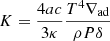
The middle panel of Fig. 2 indicates that there is more mixing in model A than in model B, as shown by the lower hydrogen mass fraction below the surface. Furthermore, the nitrogen surface enrichment in model A is significantly more pronounced than in model B, as shown in the right panel of Fig. 3. This can be attributed to the increased chemical element transport in model A, which causes a greater inward diffusion of hydrogen in the radiative zone. Therefore, for comparable Deff values, more hydrogen tends to accumulate in the layers surrounding the convective core in model A than in model B, leading to a steeper gradient in the former. This demonstrates that a model with more significant mixing in one specific region may imply steeper gradients in others.
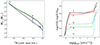 |
Fig. 3. Central and surface properties of 15 M⊙ models. Left panel: mass of the convective core in solar mass as a function of the central mass fraction of hydrogen Xc in different 15 M⊙ models. Right panel: evolution of the surface abundance ratio N/H (normalized to its initial value and in logarithmic scale) as a function of log gsurf for the same models as presented in the left panel. In both panels, the letters have the same meaning as in Fig. 2. |
The position of the MS band in the HR diagram is influenced not only by the chosen overshooting parameter, but also by the rotation physics employed. Different rotation models can shift this limit, highlighting the need to consider the rotational mixing physics when analyzing the main-sequence band. Although the convective core masses in models A and B display a comparable evolution, as illustrated in the left panel of Fig. 3, their TAMS positions are not identical (see the left panel of Fig. 2). Therefore, when calibrating models for the overshooting parameter using the TAMS position in the HR diagram, it is essential to keep in mind the potential influence of the rotation physics on this position (see the discussion in Martinet et al. 2022).
4.2.2. Impact of changing Dh
We now compare models C and D, which have the same Dshear. These models exhibit a generally higher Dh value than models A and B, but have a lower Deff value. This produces smaller convective cores, as shown in the left panel of Fig. 3. The models are less strongly mixed chemically, and this makes the tracks less luminous than those of models A and B. The difference between tracks C and D are otherwise qualitatively similar to those between models A and B. Model C, despite having a significant lower value of Deff just above the core, still shows a strong surface enrichment (see the right panel of Fig. 3). The reason is that the convective core recedes in mass, as explained above. In Fig. E.1, the tracks in the HR diagram for models E and F are compared to those of models A, B, C and D. Model E follows a very similar path as model C. Model F presents similar characteristic with model D, but it is slightly less luminous and has a bluer turnoff point.
4.2.3. Impact on the main-sequence lifetime
The MS lifetimes for the 15 M⊙ stellar models are indicated in the fourth column of Table 1. For all the models, the duration of the core hydrogen-burning phase is increased by rotation by 1−22% compared to the nonrotating model. The rotating models using the value of Dh by Maeder (2003) and the Dshear by Talon & Zahn (1997, models D and F) have the smallest increase in MS lifetime (between 1 and 6%).
4.3. Internal and surface rotations, surface abundances
In the nonmagnetic models, the main process for transporting angular momentum is meridional circulation. In all our models, we used the same equation to compute the meridional currents. Only the expression of Dh enters the equation giving U2, which appears as a multiplying factor (1 + Dh/K). However, since Dh is in general at least an order of magnitude below K in our models, the change in Dh only has a limited effect. Hence, this effect is unlikely to have a significant impact on the transport of angular momentum. The right panel of Fig. 2 shows that the internal rotation of the different models in the middle of the MS phase is quite similar. Models computed with a higher value of Dh have slightly faster rotating cores.
The time-averaged surface rotational velocity during the MS phase is indicated in the third column of Table 1. The median value is 188 km s−1. Variations of ±8% are obtained depending on the expressions used, and thus, the impact on the surface rotation rates remains modest. A change in the diffusion coefficient alters the chemical structure and thus impacts the stellar radius and mass loss by stellar winds, which in turn impacts the surface rotational velocity. However, the masses at the end of the MS phase of the different 15 M⊙ models exhibit minimum variation, with differences of approximately ±0.4%, as shown in Col. 4 of Table 1. Uncertainties in the mass-loss rates produces larger differences (Renzo et al. 2017). This explains why the differences of surface velocities remain very modest.
In contrast to the rotation rates, the surface enrichment is very sensitive to the choice of the diffusion coefficients (right panel of Fig. 3). The choice of Dshear has a greater impact on the surface enrichment compared to Deff, which governs exchanges between the convective core and the base of the radiative envelope. Models using the expression for Dshear by Maeder (1997) exhibit much stronger enrichment at the end of the MS phase than those using the expression by Talon & Zahn (1997), regardless of the chosen Dh.
4.4. He-burning lifetimes and blue-red supergiant ratios
The core He-burning lifetimes are indicated in Col. 8 of Table 1. They range from 8 to 15% of the MS lifetime. Higher values of Dh are associated with a longer core He-burning phase and larger fractions of τHe/τH.
The evolution of the effective temperature as a function of the mass fraction of helium at the center of the star for the 15 M⊙ models are shown in the left panel of Fig. 4. Only model C, and to a lesser extent, the nonrotating model G show a behavior different from that of the other models. These two models spend a significant fraction of the core He-burning phase with an effective temperature above 6000 K (log Teff > 3.8). Models that directly evolve to the red supergiant stage do so on a Kelvin-Helmholtz timescale, while those that stay longer in the blue region follow a nuclear-burning timescale. This affects the blue to red supergiant ratio and case B mass transfer in close binary evolution (see Kippenhahn & Weigert 1994; van den Heuvel 1968, for the definition of a case B mass transfer).
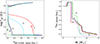 |
Fig. 4. Change is physical parameters of M⊙ models with respect to changing helium fractions. Left panel: evolution of the effective temperature as a function of the central helium abundance for different 15 M⊙ models. Right panel: helium profile vs. the mass in different 15 M⊙ models when the central helium mass fraction is 0.90. In both panels, the letters have the same meaning as in Fig. 2. |
When the mass fraction of helium at the center is 0.9, the two models exhibit the lowest helium abundance above the H-burning shell. In models with a higher helium abundance above the He-core, a red position during the core He-burning phase is favored. This is in line with what was found in Maeder & Meynet (2001) and Walmswell et al. (2015) and also in the numerical experiments by Farrell et al. (2022). It is interesting to note that the degree of mixing in the star as a whole is very different in models C and G. Despite this, they both favor a long duration in a blue supergiant phase during the first crossing of the HR gap. This indicates that the time spent in different effective temperature ranges when the star crosses the HR gap depends on changes in the distribution of the chemical elements inside the star in and near the H-burning shell. This is in line with previous works, such as those by Schootemeijer et al. (2019) and Klencki et al. (2022).
4.5. Difference in the structure at the end of the core He-burning phase
The masses of the helium and carbon-oxygen cores at the end of the core He-burning phase are shown in Cols. 14 and 15 respectively, of Table 1. The maximum relative difference in the helium core between rotating models,  , is equal to 28%. This is more than twice as large as the difference between a nonrotating model with a step overshoot of 0.25 Hp and without overshooting (see e.g. Maeder & Meynet 1987). Models with higher values of Dh show smaller helium cores at this stage. The maximum relative differences in the CO core and remnant masses between rotating models are ≈40 and 17%, respectively. These relative changes were computed the same way as for the variations in the He cores. To estimate the remnant mass, we used the relation between the CO core mass and the remnant mass from Maeder (1992). Overall, it is evident that the core sizes are significantly affected by choice of the prescription for rotation. The impact is greater than that of a moderate core overshoot in nonrotating models. These findings highlight that we need to understand the underlying physics better.
Figure 5 displays the variations in the angular velocity in different models during various evolutionary stages. The differences are minor at the end of the core H-burning phase because the equations for computing the transport of angular momentum by the meridional currents are identical and are only weakly influenced by the choice of Dh. However, changes in the chemical structure affect the tracks in the HR diagram, ultimately impacting the evolution of internal rotation. The left panel of Fig. 4 shows that the different models begin their core He-burning phase while the star is in the blue or red part of the HR diagram. Because the stars are much more compact in the blue than in the red part, large differences in angular velocity are observed among the models at the beginning of the core-He burning phase. Additionally, we would like to recall that the angular momentum transport and wind mass-loss rates for massive stars are quite uncertain and degenerate with each other for many of the aspects discussed here. The actual masses at the end of the core He-burning phase vary by nearly 30%. Regardless of the model considered, a huge ratio of the angular velocity of the core and that of the surface is observed at the end of the core He-burning phase, approximately 7−8 orders of magnitude. This indicates that fast-rotating cores are a common feature in all models that only account for the hydrodynamical instabilities induced by rotation, that is, that do not account for any magnetic instabilities.
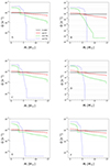 |
Fig. 5. Angular velocity profiles as a function of mass for different 15 M⊙ models at various evolutionary stages. The letters have the same meaning as in Fig. 1. |
5. The results for the 60 M⊙ models
5.1. The diffusion coefficients
In the middle of the core H-burning phase, the largest diffusion coefficient in all 60 M⊙ models is Deff (Fig. 6). This is in contrast to the 15 M⊙ models, in which Dshear was the dominating diffusion coefficient throughout the star, except just above the convective core. In the 60 M⊙ models, a very flat rotation profile develops over a very large portion of the total mass of the star due the intrinsically large convective cores and the fact that mass loss removes the radiative differentially rotating layers (see the right panel of Fig. 7). Solid-body rotation produces a large thermal imbalance because of the large deformation in the outer layers that have a rotation near the one of the core, resulting in high values of the meridional current velocities. To some extent, these models exhibit a behavior similar to that of magnetic models (Sect. 6) for the transport of the chemical species. In the magnetic model, the flat profile results from the dynamo action.
 |
Fig. 6. Variation as a function of the radius of K, the thermal diffusivity, Dconv, the convective diffusion coefficient, Dshear, the shear diffusion coefficient, Dh, the horizontal turbulence coefficient, and Deff, the effective diffusivity in different 60 M⊙ models at solar metallicity. The letters correspond to models computed with the prescription given in the second column of Table 1. The profiles are taken when the central mass fraction of hydrogen Xc = 0.35. |
 |
Fig. 7. Evolution of physical parameters of 60 M⊙ models. Left panel: evolutionary tracks in the Hertzsprung-Russell diagram. Center panel: abundance of hydrogen ranging from the center to the outer envelope of the models at Xc = 0.35 vs. the Lagrangian mass coordinate and (right panel) the variation in angular velocity as a function of the Lagrangian mass coordinate in 60 M⊙ at Z = 0.014 and with Vini/Vcrit = 0.4. The letters A to G correspond to the models as described in Table 1. |
5.2. Tracks and lifetimes
The tracks for the 60 M⊙ model and the distribution of hydrogen inside the model when the central mass fraction of hydrogen is 0.35 are shown in the left and middle panels of Fig. 7. The profiles of hydrogen shown in the middle panel correspond to positions in the HR diagram at log L/L⊙ = 5.87. Model B has the highest surface hydrogen abundance and the lowest effective temperature at this luminosity, while model C has the smallest H surface abundance and the highest effective temperature. This is expected because the closer a star approaches a chemically homogeneous structure, the bluer its position in the HR diagram. The differences are small; they are smaller than 2% and 5.5% in log L/L⊙ and in log Teff, respectively.
The differences become more important toward the end of the MS phase. The convective core masses at a given mass fraction of hydrogen at the center are higher in models C and D than in models A and B when the mass fraction of hydrogen at the center becomes lower than 0.3. These larger cores allows these two models to reach higher luminosities at the end of the MS phase (see Fig. 7). The larger convective cores are due to larger Deff in models C and D. Interestingly, in these models, the values of Dh are lower when the expression by Maeder (2003) is used instead of that of Zahn (1992). The reason is that the strong mass loss removes large amounts of angular momentum and thus decreases Ω. At the end of the MS phase, these models have lost more than 20 M⊙. The fact that Ω appears explicitly in the expressions of Dh by Maeder (2003) and Mathis et al. (2004) implies that this quantity decreases as the evolution proceeds in the 60 M⊙. This allows Deff to increase. This explains why in models C and D the convective core masses at the end of the MS phase are higher than in models A and B.
5.3. Surface velocities and abundances
The surface velocities follow a similar evolution during the MS phase, regardless of the choice of prescription (see Models A to D in the third column of Table 1). This is not the same for the surface abundances. Models C and D shows higher surface helium mass fractions than models A and B by about 20%. Since all the models end with nearly the same total mass at the end of the MS phase, this difference is mainly a result of more efficient internal mixing inside models C and D due to larger Deff.
5.4. Post-MS evolution
The nonrotating 60 M⊙ model evolves into a Wolf-Rayet star following the pathway described in the Conti scenario (Conti 1979). In the case of the rotating model, the transition into the WR phase occurs earlier. This is due to the more efficient attainment of the necessary surface abundance changes for a WR star classification, facilitated by the mixing effects of rotation. It is important to note that these results are influenced by the underlying mass-loss physics (refer to Fullerton et al. 2005; Gormaz-Matamala et al. 2023).
The upper left panel of Fig. 8 shows that the minimum luminosity reached during the WR phase for the nonmagnetic models is between 5.65 and 5.8, corresponding to variations of < 50% depending on the prescription used.
 |
Fig. 8. Evolutionary tracks in the Hertzsprung-Russell diagram (left panel), variation in the convective core mass vs. the central mass fraction of hydrogen (center panel), and the surface abundances of hydrogen, helium, carbon, nitrogen, and oxygen against the mass for models C and C*, as described in Table 1. |
Models with an initial rotation of 0.4 V/Vcrit have a shorter core He-burning lifetime by about 8 to 13% compared to nonrotating models. The difference in lifetime between the different prescription models (5%) is similar to the smallest difference between the rotating and the nonrotating models (8%). The core masses at the end of the core He-burning phase are indicated in Table 1. The more massive He-cores are those in models C and D (with the stronger mixing). They differ from models A and B by 4 M⊙ (∼20%) at most. They also have a larger CO core and higher remnant masses (assuming the star entirely collapses into a black hole). The differences are 2−3 M⊙ for the CO cores and slightly more than 1 M⊙ for the remnant mass (also a difference of 20%). While these differences are significant, these models will likely produce black holes, regardless of the choice of rotational prescription (see Fig. 3 in Ertl et al. 2020). In the context of this hotly debated topic, recent advancements in 3D neutrino-radiation hydrodynamics simulations have been significant, with multiple groups reporting that black hole (BH) formation is accompanied by successful explosions and notable mass changes. Key contributions in this area include Ott et al. (2018), Kuroda et al. (2018), Chan et al. (2020), and Burrows et al. (2023). For instance, Burrows et al. (2023) observed the formation of a 3 M⊙ BH from a 40 M⊙ progenitor. While these studies did not provide a definitive answer, they are essential for understanding the uncertainties related to rotational mixing in the context of explosion and collapse mechanisms. These uncertainties currently exceed 20%, underscoring the need for comprehensive analysis in this field.
Figure 9 shows the angular velocity inside the four models A, B, C, and D at different stages in their evolution. The behaviors in all four models are very similar, illustrating the fact that the changes in the diffusion coefficients have only an indirect impact on the internal angular velocity. In the 60 M⊙ models, much of the evolution is driven by the stellar winds. The surface velocities during the Wolf-Rayet phase are low (about 20−30 km s−1) as a result of the large mass loss. Interestingly, these models would produce BHs with a very low spin of a* ∼ 0.003. The spin parameter is equal to cJ/(GM2), where c is the velocity of light, J is the total angular momentum, G is the gravitational constant, and M is the actual mass of the star at the end of the evolution. We considered values for the end of the core He-burning phase. Some mass and angular momentum can still be lost during the advanced phases, and thus, the value quoted for a* can be slightly different for a model in the presupernova stage.
 |
Fig. 9. Variation in the angular velocity profiles as a function of mass for 60 M⊙ for models A to D and C* from left to right (see Table 1). |
6. Magnetic models
6.1. The 15 M⊙ model
The diffusion coefficients for the 15 M⊙ when the calibrated TS dynamo is used (model C*) are shown in the left panel of Fig. 10. The expressions for Dshear and Dh in the magnetic model are identical to those in the nonmagnetic model C. Therefore, we compare model C* with model C in this section. In model C*, the transport of angular momentum is dominated by the magnetic viscosity, and the transport of chemical elements is governed by the Deff coefficient, The shear diffusion coefficient has a very weak impact due to its small magnitude. Consequently, changing the expression of Dshear has no effect on chemical element transport in these models.
 |
Fig. 10. Mixing coefficients and their impact in 15 M⊙ models. Left panel: internal profiles of K, the thermal diffusivity, Dconv, the convective diffusion coefficient, Dshear, the shear diffusion coefficient, Dh, the horizontal turbulence coefficient, and Deff, the effective diffusivity in the 15 M⊙ C* model with internal magnetic fields at solar metallicity. The quantities are plotted when the central mass fraction of hydrogen Xc = 0.35. Middle panel: variation in the H-mass fraction vs. the Lagrangian mass coordinate. Right panel: variation in the angular velocity vs. mass in 15 M⊙ for the C* and C models at the end of H burning. |
The middle panel of Fig. 10 illustrates the hydrogen profile in the middle of the core H-burning phase. When compared to the nonmagnetic model (model C in red), the gradients above the core in the magnetic model are steeper and interspersed with nearly flat zones. This structure results from the receding convective core, which leaves a region of chemical gradients around it in which some mixing can occur through the action of Deff. In these regions just above the core, the mixing is not as efficient as in the region above, where the meridional currents are stronger. This therefore is an intermediate zone in which the mixing timescale is longer than the mixing timescale in the convective core and than in the radiative envelope. This tends to produce some staircase configurations. We would like to emphasize that the choice of the expression for Dh plays a key role. We present the case here for the expression by Maeder (2003). The expression of Zahn (1992) would produce a much stronger chemical mixing. These aspects will be discussed in forthcoming papers.
The left panel of the same figure shows that Deff is much larger in model C* than Dshear in model C (Fig. 1). As a result, hydrogen tends to move inward in the magnetic model, and it accumulates above the convective core due to the decrease in Deff just above the core, leading to steeper gradients. The high viscosity value results in a flat rotation profile during the middle of the MS phase, as shown in the right panel of Fig. 10.
During the MS phase, the magnetic model of the 15 M⊙ star has a wider range of effective temperatures than its nonmagnetic counterpart owing to a lower degree of mixing (left panel of Fig. 11). This weaker mixing is apparent in the evolution of the surface abundances, as shown in the middle panel of Fig. 11. The evolution of the effective temperature as a function of the mass fraction of helium in the center is shown in the right panel of Fig. 11. The magnetic model rapidly becomes a red supergiant just after the MS phase, while the nonmagnetic model burns a large part of its helium at high effective temperatures. As discussed earlier, small changes in the abundances profiles around the H-burning shell cause this difference (Walmswell et al. 2015; Klencki et al. 2022; Farrell et al. 2022). This sensitivity on small changes in the He distribution may question the robustness of this result to changes in the space and time discretization. It would go well beyond the present work to discuss this point in detail, and this possibility must therefore be kept in mind.
 |
Fig. 11. Models C and C* with a mass 15 M⊙ with Vini/Vcrit = 0.4. Left panel: evolutionary tracks in the Hertzsprung-Russell diagram during the MS phase. Middle panel: change in the nitrogen to hydrogen ratio normalized to the initial value vs. the surface gravity. Right panel: variation in the effective temperature as a function of the central helium mass fraction. |
In Fig. 12 we show the variation in the boron abundance at the surface of models A, B, C, D, and C*. As briefly mentioned in Sect. 1, boron does not need to be dredged down very deeply inside the star to be affected by nuclear reactions. It is is destroyed via proton capture at temperatures of about 6 × 10⁶ K (Proffitt et al. 1999), making it a good indicator of mixing in the outer layers of stars, where Dshear dominates in nonmagnetic models and Deff dominates in magnetic ones. Despite some differences, models A, B, C, and D exhibit similar qualitative evolution, largely because the depletion of boron primarily occurs in zone 4, where the two Dshear expressions yield comparable values. Nonetheless, the depletion of boron in magnetic models is weaker than in nonmagnetic models (at a fixed initial mass, rotation, and metallicity), which could be used to distinguish between the two types of models. Further research is necessary to investigate this possibility, but it is clear that magnetic models exhibit distinct behaviors in the boron versus log g, boron versus nitrogen surface abundances, and boron versus surface rotation planes.
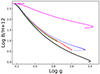 |
Fig. 12. Evolution of the B/H ratio (in number) at the surface of models A (continuous black curve), B (dashed green curve), C (dashed red curve), D (dotted blue curve), and C* (continuous magenta curve) models as a function of the surface gravity. |
In Fig. 13 we compare the angular velocity distribution of a nonmagnetic model (left panel) and a magnetic model (right panel). At the end of the core He-burning phase, the magnetic model displays a core angular velocity that is lower by three orders of magnitude than that in the nonmagnetic model. This difference suggests that the angular momentum of the remnant would decrease by three orders of magnitude, resulting in a proportional increase in its spin period. This holds assuming the angular momentum of the part of the star that becomes the neutron star remains constant post-He-burning.
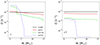 |
Fig. 13. Variation in the angular velocity as a function of the Lagrangian mass coordinate in 15 M⊙ at different evolutionary stages. The left panel shows the nonmagnetic model C. The right panel shows the magnetic model C*. |
6.2. The 60 M⊙ model
The left panel of Fig. 14 illustrates the diffusion coefficients in the magnetic 60 M⊙ model, revealing that the same trends as observed in the corresponding 15 M⊙ model also qualitatively hold in the 60 M⊙ model. Throughout the radiative zone, angular momentum transport is dominated by magnetic viscosity, while chemical species transport is dominated by Deff. Only in a small region near the surface does Dshear exceed Deff due to the differential rotation in the outermost layers (as depicted in the right panel of Fig. 14).
The profile of the hydrogen abundance in the middle of the core H-burning phase is shown in the middle panel of Fig. 14. The magnetic model retains an H-rich outer envelope, and a steep gradient connects it to the convective core. This behavior mirrors that of the magnetic 15 M⊙ model (as depicted in the middle panel of Fig. 10). The right panel of Fig. 14 shows the angular velocity variation with respect to the Lagrangian mass coordinate in the middle of the core H-burning phase. The core of the magnetic model rotates more slowly (by roughly 15% compared to the corresponding nonmagnetic model) and displays less differential rotation in the outermost layers.
The impact of magnetic instabilities on the 60 M⊙ evolutionary track is evident in the left panel of Fig. 8. Model C, which undergoes strong internal mixing, evolves almost vertically and remains in the blue, while the magnetic model evolves towards the red. As depicted in the middle panel of Fig. 8, the convective core is significantly larger in the nonmagnetic model compared to the magnetic model for most of the core H-burning phase. The right panel of Fig. 8 presents the surface abundance evolution as the actual mass of the 60 M⊙ star decreases. The hydrogen mass fraction at the surface becomes lower than 0.4 when the actual mass of the star is about 35 M⊙ in the magnetic model and about 50 M⊙ in the nonmagnetic model. Figure 15 compares the angular velocity variations at different evolutionary stages between the 60 M⊙ nonmagnetic (left panel) and magnetic (right panel) models. The strong coupling imposed by the magnetic field significantly slows down the core rotation in the magnetic model compared to the nonmagnetic model, reducing it by two orders of magnitude at the end of the core He-burning phase.
7. Discussion and conclusions
We have examined the impact of changing the expressions for the diffusion coefficients for rotation in our stellar models while keeping all other physical inputs unchanged. Our findings demonstrate that the specific choice of the expressions for Dshear and Dh in nonmagnetic models can yield markedly distinct outcomes for a given initial mass, rotational velocity, and composition. Furthermore, there are significant variations between the magnetic and nonmagnetic models. We enumerate our key findings below.
-
Altering the diffusion coefficients in nonmagnetic models does not have a significant effect on angular momentum transport, but rather impacts the stellar evolution by altering its chemical structure.
-
Regardless of the chosen diffusive coefficients or initial mass, nonmagnetic models tend to produce very rapidly rotating cores at the end of the core He-burning phase, consistent with the results of Georgy et al. (2009).
-
In magnetic models, the magnetic instability dominates angular momentum transport and is largely unaffected by the choice of Dshear and Deff. The models exhibit flat rotation profiles during the main-sequence phase for 15 and 60 M⊙ stars. Magnetic models result in significantly slower rotating cores at the end of the core He-burning phase, consistent with previous findings by Heger et al. (2005) and Fuller & Ma (2019), although their magnetic transport of angular momentum is implemented differently.
-
The choice of diffusion coefficients has a significant impact on the mixing of chemical elements and the evolutionary tracks in the HR diagram. In nonmagnetic models, changing the expression for Dshear affects the evolution of the 15 M⊙ model, but not the 60 M⊙ model. The expression for Dshear from Maeder (1997) instead of Talon & Zahn (1997) produces more luminous and bluer evolutionary tracks for the 15 M⊙ model, as well as stronger surface enrichment at the end of the MS phase.
-
Increasing Dh in the nonmagnetic 15 M⊙ model reduces the transport just above the convective core, where Deff dominates. The expression for Dh from Maeder (2003) instead of Zahn (1992) produces smaller convective cores, lower luminosity tracks, and less strongly mixed models at the end of the MS phase.
-
Reducing Deff generally leads to a decrease in mixing, but this decrease may not be significant when high values of Dshear are present in the radiative envelope above the region directly surrounding the core with strong chemical gradients during the core H-burning phase. This is due to the mild chemical gradients resulting from the retreating convective core during the early phase of the core-H-burning phase.
-
The results of the current computations are consistent with previous studies by Maeder & Meynet (2001), Walmswell et al. (2015), Klencki et al. (2022), and Farrell et al. (2022), who found that the beginning of the core He-burning phase occurs as a red supergiant when the region near the H-burning shell is enriched in helium. The timescale for the star to cross the HR gap after the MS phase plays an important role in determining the blue to red supergiant ratio and has implications for close binary evolution, particularly for case B mass transfer.
-
The differences in MS lifetimes among the rotating models computed with different diffusion coefficients are as significant as the differences between rotating and nonrotating models computed with and without a moderate core overshoot.
-
The masses of the cores at the end of He-burning also present significant differences depending on the prescriptions used. These differences may amount to twice the differences when compared against nonrotating models with and without a moderate overshoot.
-
The 60 M⊙ model is strongly affected by mass losses through stellar winds. Changing the diffusive coefficients only has a weak impact.
-
The primary process that causes the mixing of chemical elements in nonmagnetic 60 M⊙ models is Deff. Convection and mass loss cause the star to quickly transform into a body that rotates almost as solid body, leading to increased transport of chemical elements through meridional currents and consequently through Deff.
-
In models using expressions of Dh that show an explicit dependence on Ω and undergo significant mass loss, the value of Deff increases with time, leading to the development of larger convective cores at the end of the MS phase. This is because Ω decreases with time due to mass loss in these models, and as a result, Dh decreases and Deff increases.
-
Chemical mixing in magnetic models is controlled by Deff, which is affected by the choice of Dh but not by Dshear when the rotation profile is very flat. For this study, only magnetic models using the Dh from Maeder (2003) were presented. The degree of mixing in both the 15 and 60 M⊙ magnetic models is lower than that of the corresponding nonmagnetic models using the same Dh.
These changes affect the reproduction of the observed width of the MS band by a step overshoot. For instance, a lower value of step overshoot is required for Dshear from Talon & Zahn (1997) when compared to Maeder (1997). However, the calibration of convective boundary mixing must be made in conjunction with the calibration based on the chemical surface enrichment during the MS phase because the size of the convective cores also affects these changes. Model A employs the same physics as the more recent grids of stellar models by the Geneva group (Ekström et al. 2012; Georgy et al. 2013b; Groh et al. 2019; Murphy et al. 2021; Eggenberger et al. 2021; Yusof et al. 2022). The surface abundances shown by model A during the MS phase provide a reasonable match to the observed surface enrichment of stars with an average rotation velocity (as discussed in Ekström et al. 2012). The right panel of Fig. 3 indicates that models C and E would require minimal adjustments for Dshear from Maeder (1997, see middle panel of Fig. E.2). However, models B, D, and F, which use Dshear from Talon & Zahn (1997), would require either higher initial rotations or an increase in their diffusion coefficients by selecting a value for fen greater than 1.0 to achieve a similar enrichment as model A.
Although determining the optimal physics from surface observations alone remains a challenge, asteroseismic analyses of massive and low-mass stars provide valuable insights into angular momentum transport (e.g., Beck et al. 2012; Mosser et al. 2012; Deheuvels et al. 2012, 2020; Gehan et al. 2018; Salmon et al. 2022a; Pedersen 2022), while helioseismology is useful for understanding the internal rotation of the Sun (Couvidat et al. 2003). Currently, magnetic models seem to be more effective in reproducing the internal rotation of the Sun (Eggenberger et al. 2019a, 2022b), as well as that of low-mass subgiants, red giants, and clump stars (Eggenberger et al. 2019b; Moyano et al. 2022). For massive stars, fewer constraints of this nature are available, although asteroseismic data on slowly rotating β-Cephei stars have produced varied results (Salmon et al. 2022a,b). Some stars show internal angular velocity gradients that cannot be explained by existing magnetic models, while others exhibit a flat rotation profile internally. The spin of compact remnant favors very efficient angular momentum transport (Heger et al. 2004; den Hartogh et al. 2019). When both solid-body and differential rotation are observed in nature, the key challenge lies in elucidating the physical mechanisms that give rise to these two distinct rotational behaviors.
Acknowledgments
The authors would like to thank the referee for the insightful comments and contributions towards enriching this paper. We would also like to thank Yves Sibony for sharing his results on the impacts of changing the time resolution. D.N., G.M., S.E., F.D.M., P.E., C.G., and E.F. have received funding from the European Research Council (ERC) under the European Union’s Horizon 2020 research and innovation programme (grant agreement No. 833925, project STAREX). This work was supported by the Fonds de la Recherche Scientifique-FNRS under Grant No. IISN 4.4502.19.
References
- Banerjee, P., Heger, A., & Qian, Y.-Z. 2019, ApJ, 887, 187 [Google Scholar]
- Beck, P. G., Montalban, J., Kallinger, T., et al. 2012, Nature, 481, 55 [Google Scholar]
- Bogovalov, S. V., Petrov, M. A., & Timofeev, V. A. 2021, MNRAS, 502, 2409 [NASA ADS] [CrossRef] [Google Scholar]
- Brinkman, H. E., den Hartogh, J. W., Doherty, C. L., Pignatari, M., & Lugaro, M. 2021, ApJ, 923, 47 [NASA ADS] [CrossRef] [Google Scholar]
- Brinkman, H. E., Doherty, C., Pignatari, M., Pols, O., & Lugaro, M. 2023, ApJ, 951, 110 [CrossRef] [Google Scholar]
- Brott, I., de Mink, S. E., Cantiello, M., et al. 2011, A&A, 530, A115 [NASA ADS] [CrossRef] [EDP Sciences] [Google Scholar]
- Burrows, A., Vartanyan, D., & Wang, T. 2023, ApJ, 957, 68 [NASA ADS] [CrossRef] [Google Scholar]
- Chaboyer, B., & Zahn, J. P. 1992, A&A, 253, 173 [NASA ADS] [Google Scholar]
- Chan, C., Müller, B., & Heger, A. 2020, MNRAS, 495, 3751 [NASA ADS] [CrossRef] [Google Scholar]
- Chandrasekhar, S. 1933, MNRAS, 93, 390 [NASA ADS] [CrossRef] [Google Scholar]
- Chandrasekhar, S. 1961, Hydrodynamic and Hydromagnetic Stability (Oxford: Clarendon Press) [Google Scholar]
- Chatzopoulos, E., & Wheeler, J. C. 2012, ApJ, 748, 42 [NASA ADS] [CrossRef] [Google Scholar]
- Chiappini, C., Hirschi, R., Meynet, G., et al. 2006, A&A, 449, L27 [NASA ADS] [CrossRef] [EDP Sciences] [Google Scholar]
- Chieffi, A., & Limongi, M. 2013, ApJ, 764, 21 [Google Scholar]
- Choi, J., Dotter, A., Conroy, C., et al. 2016, ApJ, 823, 102 [Google Scholar]
- Choplin, A., Hirschi, R., Meynet, G., et al. 2018, A&A, 618, A133 [NASA ADS] [CrossRef] [EDP Sciences] [Google Scholar]
- Conti, P. S. 1979, in Mass Loss and Evolution of O-Type Stars, eds. P. S. Conti, & C. W. H. De Loore, 83, 431 [NASA ADS] [CrossRef] [Google Scholar]
- Couvidat, S., García, R. A., Turck-Chièze, S., et al. 2003, ApJ, 597, L77 [Google Scholar]
- de Jager, C., Nieuwenhuijzen, H., & van der Hucht, K. A. 1988, A&AS, 72, 259 [NASA ADS] [Google Scholar]
- de Mink, S. E., & Mandel, I. 2016, MNRAS, 460, 3545 [NASA ADS] [CrossRef] [Google Scholar]
- Deheuvels, S., García, R. A., Chaplin, W. J., et al. 2012, ApJ, 756, 19 [Google Scholar]
- Deheuvels, S., Ballot, J., Eggenberger, P., et al. 2020, A&A, 641, A117 [EDP Sciences] [Google Scholar]
- den Hartogh, J. W., Eggenberger, P., & Hirschi, R. 2019, A&A, 622, A187 [NASA ADS] [CrossRef] [EDP Sciences] [Google Scholar]
- Denissenkov, P. A., Ivanova, N. S., & Weiss, A. 1999, A&A, 341, 181 [NASA ADS] [Google Scholar]
- Eggenberger, P., Buldgen, G., & Salmon, S. J. A. J. 2019a, A&A, 626, L1 [NASA ADS] [CrossRef] [EDP Sciences] [Google Scholar]
- Eggenberger, P., den Hartogh, J. W., Buldgen, G., et al. 2019b, A&A, 631, L6 [NASA ADS] [CrossRef] [EDP Sciences] [Google Scholar]
- Eggenberger, P., Ekström, S., Georgy, C., et al. 2021, A&A, 652, A137 [NASA ADS] [CrossRef] [EDP Sciences] [Google Scholar]
- Eggenberger, P., Moyano, F. D., & den Hartogh, J. W. 2022a, A&A, 664, L16 [NASA ADS] [CrossRef] [EDP Sciences] [Google Scholar]
- Eggenberger, P., Buldgen, G., Salmon, S. J. A. J., et al. 2022b, Nat. Astron., 6, 788 [NASA ADS] [CrossRef] [Google Scholar]
- Ekström, S., Georgy, C., Eggenberger, P., et al. 2012, A&A, 537, A146 [Google Scholar]
- Endal, A. S., & Sofia, S. 1976, ApJ, 210, 184 [NASA ADS] [CrossRef] [Google Scholar]
- Endal, A. S., & Sofia, S. 1981, ApJ, 243, 625 [NASA ADS] [CrossRef] [Google Scholar]
- Ertl, T., Woosley, S. E., Sukhbold, T., & Janka, H. T. 2020, ApJ, 890, 51 [CrossRef] [Google Scholar]
- Espinosa Lara, F., & Rieutord, M. 2011, A&A, 533, A43 [NASA ADS] [CrossRef] [EDP Sciences] [Google Scholar]
- Farrell, E., Groh, J. H., Meynet, G., & Eldridge, J. J. 2022, MNRAS, 512, 4116 [NASA ADS] [CrossRef] [Google Scholar]
- Faulkner, J., Roxburgh, I. W., & Strittmatter, P. A. 1968, ApJ, 151, 203 [NASA ADS] [CrossRef] [Google Scholar]
- Fields, C. E. 2022, ApJ, 924, L15 [NASA ADS] [CrossRef] [Google Scholar]
- Fliegner, J., Langer, N., & Venn, K. A. 1996, A&A, 308, L13 [NASA ADS] [Google Scholar]
- Frischknecht, U., Hirschi, R., Meynet, G., et al. 2010, A&A, 522, A39 [NASA ADS] [CrossRef] [EDP Sciences] [Google Scholar]
- Frischknecht, U., Hirschi, R., Pignatari, M., et al. 2016, MNRAS, 456, 1803 [Google Scholar]
- Fuller, J., & Lu, W. 2022, MNRAS, 511, 3951 [NASA ADS] [CrossRef] [Google Scholar]
- Fuller, J., & Ma, L. 2019, ApJ, 881, L1 [Google Scholar]
- Fuller, J., Piro, A. L., & Jermyn, A. S. 2019, MNRAS, 485, 3661 [NASA ADS] [Google Scholar]
- Fullerton, A., Massa, D. L., & Prinja, R. K. 2005, J. R. Astron. Soc. Can., 99, 137 [NASA ADS] [Google Scholar]
- Gehan, C., Mosser, B., Michel, E., Samadi, R., & Kallinger, T. 2018, A&A, 616, A24 [NASA ADS] [CrossRef] [EDP Sciences] [Google Scholar]
- Georgy, C., Meynet, G., Walder, R., Folini, D., & Maeder, A. 2009, A&A, 502, 611 [NASA ADS] [CrossRef] [EDP Sciences] [Google Scholar]
- Georgy, C., Ekström, S., Eggenberger, P., et al. 2013a, A&A, 558, A103 [NASA ADS] [CrossRef] [EDP Sciences] [Google Scholar]
- Georgy, C., Walder, R., Folini, D., et al. 2013b, A&A, 559, A69 [NASA ADS] [CrossRef] [EDP Sciences] [Google Scholar]
- Gormaz-Matamala, A. C., Cuadra, J., Meynet, G., & Curé, M. 2023, A&A, 673, A109 [NASA ADS] [CrossRef] [EDP Sciences] [Google Scholar]
- Gräfener, G., & Hamann, W. R. 2008, A&A, 482, 945 [Google Scholar]
- Granada, A., & Haemmerlé, L. 2014, A&A, 570, A18 [NASA ADS] [CrossRef] [EDP Sciences] [Google Scholar]
- Griffiths, A., Eggenberger, P., Meynet, G., Moyano, F., & Aloy, M.-Á. 2022, A&A, 665, A147 [NASA ADS] [CrossRef] [EDP Sciences] [Google Scholar]
- Groh, J. H., Ekström, S., Georgy, C., et al. 2019, A&A, 627, A24 [NASA ADS] [CrossRef] [EDP Sciences] [Google Scholar]
- Heger, A., Langer, N., & Woosley, S. E. 2000, ApJ, 528, 368 [NASA ADS] [CrossRef] [Google Scholar]
- Heger, A., Woosley, S. E., Langer, N., & Spruit, H. C. 2004, in Stellar Rotation, eds. A. Maeder, & P. Eenens, 215, 591 [NASA ADS] [Google Scholar]
- Heger, A., Woosley, S. E., & Spruit, H. C. 2005, ApJ, 626, 350 [Google Scholar]
- Hirschi, R., Meynet, G., & Maeder, A. 2004, A&A, 425, 649 [NASA ADS] [CrossRef] [EDP Sciences] [Google Scholar]
- Hirschi, R., Meynet, G., & Maeder, A. 2005a, A&A, 433, 1013 [NASA ADS] [CrossRef] [EDP Sciences] [Google Scholar]
- Hirschi, R., Meynet, G., & Maeder, A. 2005b, A&A, 443, 581 [NASA ADS] [CrossRef] [EDP Sciences] [Google Scholar]
- Keszthelyi, Z., Meynet, G., Shultz, M. E., et al. 2020, MNRAS, 493, 518 [NASA ADS] [CrossRef] [Google Scholar]
- Kippenhahn, R., & Thomas, H. C. 1970, in IAU Colloq. 4: Stellar Rotation, ed. A. Slettebak, 20 [CrossRef] [Google Scholar]
- Kippenhahn, R., & Weigert, A. 1994, Stellar Structure and Evolution (Berlin, Heidelberg: Springer-Verlag) [Google Scholar]
- Kippenhahn, R., Meyer-Hofmeister, E., & Thomas, H. C. 1970, A&A, 5, 155 [Google Scholar]
- Klencki, J., Istrate, A., Nelemans, G., & Pols, O. 2022, A&A, 662, A56 [NASA ADS] [CrossRef] [EDP Sciences] [Google Scholar]
- Kong, D., Zhang, K., & Schubert, G. 2015, MNRAS, 448, 456 [NASA ADS] [CrossRef] [Google Scholar]
- Krtička, J., Owocki, S. P., & Meynet, G. 2011, A&A, 527, A84 [NASA ADS] [CrossRef] [EDP Sciences] [Google Scholar]
- Kuroda, T., Kotake, K., Takiwaki, T., & Thielemann, F.-K. 2018, MNRAS, 477, L80 [NASA ADS] [CrossRef] [Google Scholar]
- Limongi, M., & Chieffi, A. 2018, ApJS, 237, 13 [NASA ADS] [CrossRef] [Google Scholar]
- Maeder, A. 1987, A&A, 178, 159 [NASA ADS] [Google Scholar]
- Maeder, A. 1992, A&A, 264, 105 [NASA ADS] [Google Scholar]
- Maeder, A. 1997, A&A, 321, 134 [NASA ADS] [Google Scholar]
- Maeder, A. 1999, A&A, 347, 185 [NASA ADS] [Google Scholar]
- Maeder, A. 2002, A&A, 392, 575 [NASA ADS] [CrossRef] [EDP Sciences] [Google Scholar]
- Maeder, A. 2003, A&A, 399, 263 [NASA ADS] [CrossRef] [EDP Sciences] [Google Scholar]
- Maeder, A., & Meynet, G. 1987, A&A, 182, 243 [NASA ADS] [Google Scholar]
- Maeder, A., & Meynet, G. 2001, A&A, 373, 555 [NASA ADS] [CrossRef] [EDP Sciences] [Google Scholar]
- Maeder, A., & Meynet, G. 2005, A&A, 440, 1041 [NASA ADS] [CrossRef] [EDP Sciences] [Google Scholar]
- Maeder, A., & Meynet, G. 2012, Rev. Mod. Phys., 84, 25 [Google Scholar]
- Maeder, A., & Zahn, J.-P. 1998, A&A, 334, 1000 [NASA ADS] [Google Scholar]
- Mandel, I., & de Mink, S. E. 2016, MNRAS, 458, 2634 [NASA ADS] [CrossRef] [Google Scholar]
- Marchant, P., & Moriya, T. J. 2020, A&A, 640, L18 [EDP Sciences] [Google Scholar]
- Martinet, S., Meynet, G., Nandal, D., et al. 2022, A&A, 664, A181 [NASA ADS] [CrossRef] [EDP Sciences] [Google Scholar]
- Mathis, S., Palacios, A., & Zahn, J. P. 2004, A&A, 425, 243 [NASA ADS] [CrossRef] [EDP Sciences] [Google Scholar]
- Mendel, J. T., Venn, K. A., Proffitt, C. R., Brooks, A. M., & Lambert, D. L. 2006, ApJ, 640, 1039 [NASA ADS] [CrossRef] [Google Scholar]
- Meynet, G., & Maeder, A. 1997, A&A, 321, 465 [NASA ADS] [Google Scholar]
- Meynet, G., & Maeder, A. 2000, A&A, 361, 101 [NASA ADS] [Google Scholar]
- Meynet, G., & Maeder, A. 2002, A&A, 381, L25 [NASA ADS] [CrossRef] [EDP Sciences] [Google Scholar]
- Meynet, G., & Maeder, A. 2005, A&A, 429, 581 [CrossRef] [EDP Sciences] [Google Scholar]
- Meynet, G., Eggenberger, P., & Maeder, A. 2011, A&A, 525, L11 [CrossRef] [EDP Sciences] [Google Scholar]
- Meynet, G., Ekstrom, S., Maeder, A., et al. 2013, in Lecture Notes in Physics, eds. M. Goupil, K. Belkacem, C. Neiner, F. Lignières, & J. J. Green (Berlin: Springer-Verlag), 865, 3 [NASA ADS] [CrossRef] [Google Scholar]
- Mosser, B., Goupil, M. J., Belkacem, K., et al. 2012, A&A, 548, A10 [NASA ADS] [CrossRef] [EDP Sciences] [Google Scholar]
- Moyano, F. D., Eggenberger, P., Meynet, G., et al. 2022, A&A, 663, A180 [NASA ADS] [CrossRef] [EDP Sciences] [Google Scholar]
- Müller, P. E., & Vink, J. S. 2014, A&A, 564, A57 [CrossRef] [EDP Sciences] [Google Scholar]
- Murphy, L. J., Groh, J. H., Ekström, S., et al. 2021, MNRAS, 501, 2745 [NASA ADS] [CrossRef] [Google Scholar]
- Nguyen, C. T., Costa, G., Girardi, L., et al. 2022, A&A, 665, A126 [NASA ADS] [CrossRef] [EDP Sciences] [Google Scholar]
- Nugis, T., & Lamers, H. J. G. L. M. 2000, A&A, 360, 227 [NASA ADS] [Google Scholar]
- Ott, C. D., Roberts, L. F., da Silva Schneider, A., et al. 2018, ApJ, 855, L3 [NASA ADS] [CrossRef] [Google Scholar]
- Palacios, A., Talon, S., Charbonnel, C., & Forestini, M. 2003, A&A, 399, 603 [CrossRef] [EDP Sciences] [Google Scholar]
- Palacios, A., Meynet, G., Vuissoz, C., et al. 2005, A&A, 429, 613 [NASA ADS] [CrossRef] [EDP Sciences] [Google Scholar]
- Pauli, D., Langer, N., Aguilera-Dena, D. R., Wang, C., & Marchant, P. 2022, A&A, 667, A58 [NASA ADS] [CrossRef] [EDP Sciences] [Google Scholar]
- Pedersen, M. G. 2022, ApJ, 940, 49 [NASA ADS] [CrossRef] [Google Scholar]
- Pignatari, M., Gallino, R., Meynet, G., et al. 2008, ApJ, 687, L95 [Google Scholar]
- Pitts, E., & Tayler, R. J. 1985, MNRAS, 216, 139 [NASA ADS] [CrossRef] [Google Scholar]
- Prat, V., Guilet, J., Viallet, M., & Müller, E. 2016, A&A, 592, A59 [NASA ADS] [CrossRef] [EDP Sciences] [Google Scholar]
- Proffitt, C. R., & Quigley, M. F. 2001, ApJ, 548, 429 [NASA ADS] [CrossRef] [Google Scholar]
- Proffitt, C. R., Jönsson, P., Litzén, U., Pickering, J. C., & Wahlgren, G. M. 1999, ApJ, 516, 342 [NASA ADS] [CrossRef] [Google Scholar]
- Proffitt, C. R., Lennon, D. J., Langer, N., & Brott, I. 2016, ApJ, 824, 3 [NASA ADS] [CrossRef] [Google Scholar]
- Renzo, M., & Götberg, Y. 2021, ApJ, 923, 277 [NASA ADS] [CrossRef] [Google Scholar]
- Renzo, M., Ott, C. D., Shore, S. N., & de Mink, S. E. 2017, A&A, 603, A118 [NASA ADS] [CrossRef] [EDP Sciences] [Google Scholar]
- Renzo, M., Zapartas, E., Justham, S., et al. 2023, ApJ, 942, L32 [NASA ADS] [CrossRef] [Google Scholar]
- Salmon, S. J. A. J., Moyano, F. D., Eggenberger, P., Haemmerlé, L., & Buldgen, G. 2022a, A&A, 664, L1 [NASA ADS] [CrossRef] [EDP Sciences] [Google Scholar]
- Salmon, S. J. A. J., Eggenberger, P., Montalbán, J., et al. 2022b, A&A, 659, A142 [NASA ADS] [CrossRef] [EDP Sciences] [Google Scholar]
- Schootemeijer, A., Langer, N., Grin, N. J., & Wang, C. 2019, A&A, 625, A132 [NASA ADS] [CrossRef] [EDP Sciences] [Google Scholar]
- Shu, F. H. 1992, The Physics of Astrophysics. Volume II: Gas Dynamics (Mill Valley: University Science Books) [Google Scholar]
- Song, H. F., Meynet, G., Maeder, A., Ekström, S., & Eggenberger, P. 2016, A&A, 585, A120 [NASA ADS] [CrossRef] [EDP Sciences] [Google Scholar]
- Spitzer, L. 1956, Physics of Fully Ionized Gases (New York: Interscience) [Google Scholar]
- Spruit, H. C. 1999, A&A, 349, 189 [NASA ADS] [Google Scholar]
- Spruit, H. C. 2002, A&A, 381, 923 [CrossRef] [EDP Sciences] [Google Scholar]
- Sylvester, R. J., Skinner, C. J., & Barlow, M. J. 1998, MNRAS, 301, 1083 [Google Scholar]
- Talon, S., & Zahn, J. P. 1997, A&A, 317, 749 [NASA ADS] [Google Scholar]
- Talon, S., Zahn, J. P., Maeder, A., & Meynet, G. 1997, A&A, 322, 209 [NASA ADS] [Google Scholar]
- Tayler, R. J. 1973, MNRAS, 161, 365 [CrossRef] [Google Scholar]
- van den Heuvel, E. P. J. 1968, Utrechtse Sterrekundige Overdrukken, 102, 16 [Google Scholar]
- van Loon, J. T., Groenewegen, M. A. T., de Koter, A., et al. 1999, A&A, 351, 559 [NASA ADS] [Google Scholar]
- Venn, K. A., Brooks, A. M., Lambert, D. L., et al. 2002, ApJ, 565, 571 [NASA ADS] [CrossRef] [Google Scholar]
- Vink, J. S., de Koter, A., & Lamers, H. J. G. L. M. 2001, A&A, 369, 574 [NASA ADS] [CrossRef] [EDP Sciences] [Google Scholar]
- von Zeipel, H. 1924, MNRAS, 84, 665 [NASA ADS] [CrossRef] [Google Scholar]
- Walmswell, J. J., Tout, C. A., & Eldridge, J. J. 2015, MNRAS, 447, 2951 [NASA ADS] [CrossRef] [Google Scholar]
- Yoon, S. C., Langer, N., & Norman, C. 2006, A&A, 460, 199 [NASA ADS] [CrossRef] [EDP Sciences] [Google Scholar]
- Yusof, N., Hirschi, R., Eggenberger, P., et al. 2022, MNRAS, 511, 2814 [NASA ADS] [CrossRef] [Google Scholar]
- Zahn, J.-P. 1992, A&A, 265, 115 [NASA ADS] [Google Scholar]
Appendix A: A brief discussion of the physics of rotation
For the sake of completeness, we recall here a few points about the physics of rotation included in our models. In models without magnetic fields, the angular momentum is mainly transported by meridional currents, while the chemical species are transported by shear instabilities and meridional currents.
The transport of angular momentum by the meridional currents is computed by resolving an advecto-diffusive equation (see Eq. 2) during the MS phase. After the MS phase, a diffusive approach is applied because the structure becomes too complex with an intermediate convective zone to allow us to resolve the advecto-diffusive equation. This shortcoming can be overcome, however, because the timescales during the post-MS phases are reduced and one of the dominant effects governing the change in the angular velocity inside the star in the hydrodyanmical model is the local conservation of the angular momentum. In some models, the transport of angular momentum by the meridional currents is computed by resolving a diffusive equation (see e.g. Heger et al. 2000; Chieffi & Limongi 2013; Choi et al. 2016; Nguyen et al. 2022), and in others, the advecto-diffusive equation was resolved (Talon et al. 1997; Meynet & Maeder 2000; Palacios et al. 2003; Chieffi & Limongi 2013). We note that Chieffi & Limongi (2013) implemented both the advecto-diffusive and the diffusive equation for the transport of angular momentum, but most of the results presented in this paper were obtained with the diffusive approach. We recall a few points here. First, the transport by meridional currents is an advective process, and in principle, it should therefore be accounted for by resolving such an equation. A diffusive equation predicts a much flatter distribution of the angular velocity during the MS phase, as is shown in Fig. 1 in Griffiths et al. (2022).
Our models explicitly account for an expression for the strong horizontal shear diffusion Dh (Zahn 1992; Maeder 2003; Mathis et al. 2004). Some authors (see e.g. Heger et al. 2000; Choi et al. 2016; Nguyen et al. 2022) did not explicitly account for an explicit expression for Dh, although they implicitly accounted for it assuming that a process causes the shellular rotation state that is assumed by any 1D stellar evolution model with rotation. Interestingly, Dh is involved in the expression of Dshear of Talon & Zahn (1997) as a factor that reduces the inhibiting effect of the chemical stratification. It thus replaces the use of a constant value parameter (often called fμ) that multiplies the μ gradients, that is, those that replace ∇μ by fμ∇μ, with fμ having a value of about one percent in the criterion that gives the lower limit of the shear, enabling the instability to be activated (Heger et al. 2000). The value of this parameter is chosen for compatibility of models with an averaged surface rotation with the observations to reproduce some surface nitrogen enrichment at the end of the MS phase Chieffi & Limongi (see e.g. Sect. 3 in 2013). Another effect of considering an explicit expression for Dh is that it naturally allows us to account for the different efficiencies of the meridional currents in transporting angular momentum and the chemical species. This comes from the expression of Deff (see Eq. 8). In this expression, the factor 1/30 is not a free parameter. It simply comes from the computation of  , where P2(cos θ) = 0.5(3cos3θ − 1) (Chaboyer & Zahn 1992). For the transport by shear, the efficiency appears to be the same for the angular momentum and the chemical species, according to the simulation by Prat et al. (2016).
In our approach, the free parameters are on the one hand, the fraction of the energy used to drive the transport and the numerical parameters in front of the expressions of the strong horizontal diffusion. For the first, we chose to consider here that the whole energy is used to trigger the mixing. This parameter can be interpreted in two ways: as the fraction of the excess energy in the shear that can be used for the transport for a given critical Richardson number, or as a value for the critical Richardson number given a fraction of the energy in the shear that can be used for the transport Maeder (see Eq. 2.2 in 1997, for the expression of the Richardson criterion). The Richardson number is a dimensionless number defined as the ratio of the buoyancy term to the flow shear term. The critical value is the minimum value for the medium to become turbulent. The value of 0.25 is explained, for instance, in Shu (1992). Regardless of the choice made here, there is no reason to change the assumption depending on the expressions used, provided they are based on the same general physical assumptions, which is the case here. We adopted the numerical parameters in front of expression Dh as suggested by the authors that proposed this expressions because these authors chose these numerical factor based on physical arguments. Thus, we are left with a completely determined system that allows us to compute models that can be compared because they are based on similar physical assumption.
For the magnetic models, the main mechanism for the transport of the angular momentum is the magnetic viscosity, as described by Spruit (1999, 2002), and Heger et al. (2005). In these models, we did not account for the angular momentum transport by the meridional currents. Meridional currents have little effect on the redistribution of the angular momentum. These currents would transport angular momentum from the outer regions of the star into the inner regions most of the time, and accounting for them requires the use of very small time steps when applied to fast-rotating massive stars (Maeder & Meynet 2005). We chose to not account for this transport in our models. In these models, the mixing of the chemical elements is mainly driven by Deff, and thus, by the concomitant effect of meridional circulation and the strong horizontal shear turbulence. The Tayler–Spruit calibrated magnetic models have the value CT and (as for the nonmagnetic models), the numerical parameters in front of the expressions of the strong horizontal diffusion as free parameters. Here, we present models with the expression and the numerical values given in Maeder (2003).
Finally, we add that all the models begin their evolution with a flat profile of Ω at the ZAMS. The initial distribution of the angular velocity in nonmagnetic models very rapidly converges toward an equilibrium profile, so that the inward transport by merdional currents is balanced by the outward transport by shear (see the discussion in Denissenkov et al. 1999; Meynet & Maeder 2000). Granada & Haemmerlé (2014) also discussed that starting on the ZAMS with a differential rotation profile or from a solid-body rotation profile gives a similar evolution as long as the total angular momentum of the model is the same. For magnetic models, the coupling due to the magnetic instability is so strong (especially at the beginning, when there no inhibiting μ–gradients) that starting from profiles different from a solid-body profile would not change the flat rotation profile that the star eventually shows.
Appendix B: Physical ingredients of the stellar models
We adopted the same physical ingredients as in Ekström et al. (2012). We recall some of main properties here. The models were computed with a step overshooting. The radius of the convective core is given by RSchw + 0.1 Hp, where RSchw is the radius of the convective core given by the Schwarzschild criterion for convection, and Hp is the pressure scale height estimated at that position. We accounted for this step overshooting during the core H- and He-burning phases. We did not account for any overshooting for intermediate convective zones or at the bottom of the outer convective zone.
The mass-loss rate scheme is described in detail in Sect. 2.6 of Ekström et al. (2012). During the MS phase, the prescription by Vink et al. (2001) was used. In the domain not covered by this prescription, we used the fit proposed by de Jager et al. (1988). This last prescription implicitly accounts for an increase in the mass flux when the model enters the observed luminosity and effective temperature domain corresponding to luminous blue variables. For red supergiants with log Teff < 3.7, a linear fit between the data by Sylvester et al. (1998) and those of van Loon et al. (1999) was used. During the Wolf-Rayet phase, the prescription by Nugis & Lamers (2000) was adopted. In the small domain where the prescription by Gräfener & Hamann (2008) is valid, it was preferred to that of Nugis & Lamers (2000). The correcting factor due to rotation was accounted for as proposed by Meynet & Maeder (2000).
No thermohaline mixing or semiconvection was considered. Chemical elements are homogeneously mixed in convective zones. In rotating models, some mixing also occurs in radiative regions induced by rotation.
The time steps were controlled by the nuclear energy generation inside the star and were additionally limited by the change in the main physical quantities such as the central fuel abundance, Teff, ρc, critical rotation, and transport of Ω. The space resolution was chosen so that the gradients with respect to the Lagrangian mass coordinate in all the main structure quantities such as the pressure, temperature, luminosity, and radius were below some predefined values.
Appendix C: Resolution tests
This appendix presents our findings from the resolution tests conducted using HR diagrams. We studied four 15 M⊙ models without rotation, as shown in Figure C.1. These models are crucial for understanding numerical convergence in computational stellar physics. There are two groups of models based on their time-step sizes. The first group, with the largest time steps, is shown with solid lines. The evolution of this group was traced until the onset of core helium-burning. The second group, with time steps 10 to 100 times smaller, is shown with dashed lines. For this group, we only traced the evolution up to just past the main sequence due to long computational times and early divergence. The analysis of these models shows that changing the time-step size alters the blue turnoff effective temperature and luminosity by about 0.02 dex. Therefore, any differences smaller than this between models computed with different physics is likely not relevant because it can be due to the difference in discretization rather than caused by a difference in the physics. These changes highlight the limitations of our computations.
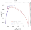 |
Fig. C.1. HR diagram for four (Ledoux and Schwarzschild, long and short timescales) 15 M⊙ models without rotation, showing a comparison of the effect of the time resolution on evolution. |
Appendix D: Smoothing of dΩ/dr
Meridional circulation in GENEC implies the fourth-order derivative of Ω, and this was obtained by performing a polynomial fit on a sliding window. The polynomial itself was of second order, and we used the NAG subroutine e02acf to calculate it. The size of the window was determined by the number of shells max (5, number of shells/120). This fitting of the run of Ω was only used to compute the derivative of Ω with respect to r, but it does not replace the actual value of Ω obtained from the resolution of the transport equations.
Appendix E: Figures for prescriptions E and F
We discuss here the models computed with Dh of Mathis et al. (2004) and compare them with the models computed with Dh of Maeder (2003).
Figure E.1 is the analog of Fig. 2 for models C, D, E and F. Models C and E (using Dshear of Maeder 1997), but different Dh expression (C is the expression by Maeder 2003, and E is the expression of Mathis et al. 2004) have very similar evolutionary tracks (see the left panel). Model C shows a slightly smoother gradient of hydrogen than model E.
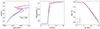 |
Fig. E.1. Variation of physical parameters in the 15 M⊙ models. Left panel: Evolutionary tracks during the MS phase in the Hertzsprung-Russell diagram for models C, D, E, and F (see Table 1) as a function of the Lagrangian mass for the 15 M⊙ at Z = 0.014 and with Vini/Vcrit = 0.4. Middle panel: Abundance of hydrogen in mass fraction ranging from the center to the outer envelope of the models when the central mass fraction of hydrogen is Xc = 0.35. Right panel: Variations in the angular velocity vs. the mass coordinate for the same models as are shown in the middle panel. |
Models F and D use Dshear of Talon & Zahn (1997) with the two different Dh. They present steeper chemical gradients above the convective core than models C and E, which use Dshear by Maeder (1997). This illustrates the fact that the choice Dshear impacts the degree of the chemical mixing.
The angular velocity profiles of all these four models are nearly indistinguishable, illustrating the fact that the choice of Dshear and Dh has little impact on the angular momentum transport in the star. For the initial rotation considered here, the changes in the chemical mixing do not change the evolution so much as to indirectly impact the profile of Ω.
The evolution of the convective core masses are compared in the right panel of Fig. E.2. They do not show any striking differences. On the other hand, the surface enrichments are significantly different between these models (see the middle panel of Fig. E.2). Globally, the models using Dshear of Maeder (1997) (C and E) are more strongly mixed than those using Dshear of Talon & Zahn (1997) (D and F).
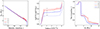 |
Fig. E.2. Additional physical parameters during the evolution of various 15 M⊙ models. Left panel: Evolution of the convective core mass during the MS phase as a function of central mass of hydrogen. Center panel: Abundance ratio of nitrogen and hydrogen at the surface normalized to their initial values vs. the surface gravity. Right panel: Profile of the helium mass fraction against the mass coordinate when the central helium fraction Yc is 0.90. The letters C to F correspond to the models with different prescriptions as described in Table 1. |
The abundances of helium as a function of the Lagrangian mass coordinate when the mass fraction of helium at the center is 0.9 are shown in the right panel of Fig. E.2. The profiles of models E and F are very similar to the profile in model C. We therefore expect that these models will spend a fraction of their core He-burning phase in a blue region of the HR diagram, which is indeed the case (see Fig. E.3). This supports the view that any helium enrichment in the H-burning shell tends to produce an evolution toward the red supergiant stage along a Kelvin-Helmholtz timescale.
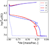 |
Fig. E.3. Evolution of the effective temperature as a function of the mass fraction of helium at the center during the core He-burning phase for models C, D, E, and F. |
Appendix F: Hydrostatic effects
Rotation imposes through the centrifugal force a hydrostatic structure different from the one of non-rotating models (Chandrasekhar 1933; Kong et al. 2015). Indeed the spherical symmetry is broken and the star will get an oblate shape due to rotation. At the surface, the surface deformation thus implies change of the brightness and colors with the latitude (von Zeipel 1924; Espinosa Lara & Rieutord 2011). To plot the tracks in the HR diagrams, we use the bolometric luminosity and a surface averaged effective temperature for respectively L and Teff. The surface averaged effective temperature is obtained by the relation  , where L is the luminosity of the star, R, the radius of a sphere that would have the same surface, S, as the deformed star. Note that the actual observed luminosity depends on inclination since a fast rotating star is brighter seen pole on than when seen equator on. However the rotations considered here are too small for this effect being important.
The deformation of the star also imposes that the mechanical equilibrium is different from the one of a non-rotating star. To account for these hydrostatic effects, we follow the method proposed by Kippenhahn & Thomas (1970). The justification for using this method that is exact only in case of a cylindral distribution of the angular velocity to the case of shellular rotation where the angular velocity is constant on isobaric surface is discussed in Meynet & Maeder (1997).
Appendix G: Equations for the advection of angular momentum
The equation for the transport of the chemical species is a pure diffusive equation, the one for the angular momentum is an advecto-diffusive equation. Actually before any simplifications that are valid only for the chemical species, both transport equations are advecto-diffusive equations. As demonstrated by Chaboyer & Zahn (1992), the advecto-diffusive equation for the transport of the chemical species reduces to a pure diffusive equations in the case of a strong horizontal turbulence. Such a simplification cannot be done for the transport of the angular momentum by the meridional currents. This is due to the fact that the quantity of angular momentum that is transported vertically depends on the distance to the rotational axis. This is not the case for the chemical species. It is very important to keep the advecto-diffusive form of the equation describing the transport of the angular momentum by the meridional currents when the transport by meridional currents dominates. (e.g. in rotating massive stars during the core Hydrogen burning phase without any dynamo effect). Let us reminds that an advecto-diffusive equation can transport a quantity from a region where this quantity is abundant to a region where it is less abundance (like does a diffusive equation). But it can also transport in the reverse direction reinforcing the gradient of that quantity between two regions (a process that a diffusion process cannot do). Thus describing the transport by meridional currents by a diffusive equation may not only make errors on the strengths of the transport but also on its sign.
When the advective part of the equation needs to be resolved (in non-magnetic models during the core H-burning phase, see discussion later), we actually resolve a system of four differential equations:
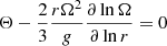 (G.1)
(G.1)
 (G.2)
(G.2)
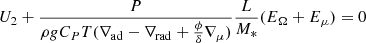 (G.3)
(G.3)
 (G.4)
(G.4)
with Λ = r∇μ/(6Hp), M* = L/[Mr(1 − Ω2/[2πGρ])], and
![Mathematical equation: $$ \begin{aligned}&E_\Omega +E_\mu =2\left[1-{\Omega ^2 \over 2\pi G \rho } -{\epsilon \over \epsilon _m}\right] {\tilde{g} \over g} \end{aligned} $$](/articles/aa/full_html/2024/04/aa46979-23/aa46979-23-eq35.gif)
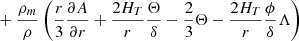
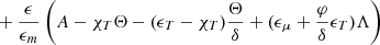
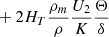
The four unknowns (Θ, A, U2, Ω) are obtained resolving this system of differential equations using a Henyey method with the appropriate boundary conditions
Appendix H: Simplified expression of the meridional velocity
In some circumstances, merdional currents contribute little to the transport of the angular momentum. Typically after the MS phase, the evolutionary timescales are short enough for the specific angular momentum be little changed by meridional currents or when the dynamo theory is accounted for, the dominating process is the magnetic coupling and no longer the meridional currents for the transport of the angular momentum). In those cases, we still need an expression for U2 that enters into the diffusion coefficients (see below). In those case we use the follwing simplified expression for U2
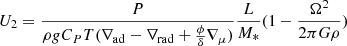 (H.1)
(H.1)
Appendix I: Hydrodynamical instabilities triggered by rotation in radiative zones
In non-magnetic models, even starting with a solid body rotation, very rapidly radial/horizontal gradients of angular velocity will appear inside the star as a result of the change of the chemical composition and of the internal structure due to nuclear burning, the loss at the surface of energy through the luminosity and of angular momentum by mass loss. These internal gradients at their turn trigger turbulence that transports both chemical species and angular momentum. These transport are however likely very anisotropic. Indeed, along the radial direction and in radiative zones, the instabilities have to overcome the stabilizing effect of the temperature and chemical composition gradients (an effect often called the stratification of the medium or the entropy gradient). The vertical transports are therefore reduced compared to what happens along the horizontal direction, i.e. along an equipotential or an isobar (in case the centrifugal force is conservative equipotentials are equivalent to isobars. This is not the case of a shellular distribution of the angular velocity, then we can only speak of isobaric surface), where no such counteracting effects exists and the turbulence is thus much stronger.
These considerations led Zahn (1992) to build a consistent description of the interactions between meridional currents and shear instabilities based on a single a priori hypothesis that the strong horizontal turbulence brings the star in a state of shellular rotation in which each isobaric layer show values of Ω that are nearly constant. Further improvements of the theory have been made by Maeder & Zahn (1998). By nearly constant, we mean here that the variation of Ω along the isobaric surfaces are very small and can be accounted for by retaining only the first term in a development of Ω as a function of Legendre polynomials. The same is true for the temperatures, densities, chemical compositions on those surfaces. This is what has been called shellular models.
These types of models can be well described by 1D models. Indeed the stellar structure equations can be modified following the method adapted from the one of Kippenhahn & Thomas (1970) by Meynet & Maeder (1997) to provide solutions for the mean values of the stellar structure properties in each layers. Some reconstruction of the variations of these quantities with the latitude can be obtained using developments in Legendre polynomials. This is why, sometimes these models are described as 1.5D models.
Appendix J: Physical basis for the different shear diffusion coefficients
The transport processes for being active needs to overcome some stabilizing effects. This is expressed by necessary conditions that have to be fullfilled for a given instability to become active. These conditions can be deduced by comparing the energy required to accomplish the transport of a fluid element to the available free energy that can be used for that purpose. In non-magnetic model, the condition is the Richardson criterion (see Chandrasekhar 1961). It expresses the requirement that the excess energy coming from the differential rotation that can be used to drive the instability needs to overcome the temperature and chemical composition gradients (or entropy gradient). It can be written (see e.g. Eq. 2.2 in Maeder 1997)
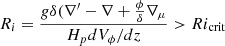 (J.1)
(J.1)
where Ri is the Richardson number, ∇′ and ∇ respectively the thermal gradients inside the fluid element and in the surrounding medium (∂lnT/∂lnP, with T and P the temperature and pressure), ∇μ the gradient of the mean molecular in the surrounding medium, g the gravity, Hp the pressure scale height, and dVϕ/dz the differential azimuthal velocity with respect to a direction perpendicular to the isobaric surface, δ = −(∂lnρ/∂lnT)P, μ, ϕ = (∂lnρ/∂lnμ)P, T. The critical Richardson number is often taken equal to 1/4 but its value is pertained with some uncertainty and can be as high as 1.0. As explained in the next section, the Richardson criterion is actually included into the expressions used for the vertical shear diffusion coefficient.
Let us remind that in Meynet & Maeder (1997) it has been shown that a strict application of the Richardson criterion prevent any transport of the chemical elements in radiative zones where μ-gradients are present. This was due to the fact that the amplitude of the differential rotation was never high enough in regions of mean molecular weight gradient for allowing the instability to appear.
Maeder (1997) has suggested that due to the fact that the medium is anyway turbulent along the horizontal direction and that this turbulence will have some radial component, it was too restrictive to use strictly the Richardson criterion that is actually valid starting from a non-turbulent medium. The turbulence already present allows the excess energy in the differential rotation to be always used for producing a mixing limited by the amount of excess energy available in the shear. In that case there is no longer a criterion that allows the instability to be active, thus no longer an on/off behavior. Rather a mixing is always present whose strength however depends on the amount of energy that can be used to drive it. This lead to a new formulation of the diffusion coefficient driving the transport of both the chemical elements and the angular momentum by shear (see Sect. 3).
Talon & Zahn (1997) proposed a similar idea although leading to a different expression. These authors explicitely accounted for the effect of the strong horizontal turbulence (that is always present in rotating models), to weaken the μ-gradients. Indeed, the strong horizontal turbulence decreases the differences between the mean molecular weight characterizing the interior of the fluid element from that of the surrounding medium. This tends to favor the instability since for an upward moving element, the drawback force due to the μ-stratification will be diminished. The expression for Dshear deduced from this approach is given in Sect. 3.
The horizontal shear diffusion, Dh is the diffusion coefficient that describes the transport due to the horizontal turbulence along the isobaric surfaces.
The coefficient Dh describes, as reminded above, a strong turbulence. Its expression is difficult to be obtained from first principles. Since the horizontal differential rotation is driven mainly by meridional currents, its expression contains a dependance on the meridional velocities. Consideration linked to physical units are also used as well as guidance from experiments. The interested reader will find the discussion of the different expressions so far published in the literature in the respective papers (see the references below).
A condition however that Dh should fullfill is that it should be strong enough to indeed impose shellular rotation. This implies that the timescale for producing a nearly constant value of Omega along an isobaric surface should be much shorter than any process like meridional currents tending to create different values of Ω at different latitude along an isobar.
Also, one expects that Dh is larger than Dshear. Indeed, any shear instability along a direction perpendicular to an isobar faces the counteracting effect of the stabilizing effects of the density and temperature gradients. As a result, the shear turbulence along that direction is weaker than along an isobar and the diffusion coefficient describing it, the shear diffusion coefficient, Dshear is much weaker that Dh.
Appendix K: Magnetic models
This diffusivity comes from the fact that magnetic fields are produced by electrical currents that encounters some resistivity in the medium, thus transforming part of the energy into thermal ones. The expression for ohmic diffusion involves a description of how an electron can be deflected by charge along its path. This scatter not only modifies the current and hence the magnetic field but also induce some mixing of elements.
In case it not triggered, i.e. when the shear q is smaller than a minimum value qmin where qmin is
 (K.1)
(K.1)
in which η, the diffusion coefficient appears.
When the condition for the instability is realized (using in qmin for η the value valid in absence of any instability), a new value of η has to be computed. It is obtained resolving the system of two equations below. The first one results from equating two timescales: the amplification timescale defined as the time needed to amplify the radial magnetic field to an azimuthal magnetic field whose amplitude would be equal to the already existing one. It writes
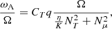 (K.2)
(K.2)
where...
The second one results on a condition on the lengthscale of the instability. This lengthscale should be large enough for not being quickly damped by the magnetic diffusivity and small enough for the free energy available (due to shear) to overcome the stabilizing effect of the entropy gradient.
 (K.3)
(K.3)
where... This above equation has two unknowns, ωA and η. Resolving these two equations give values for ωA (or BΦ) and η.
It is easy to show that replacing the expression of ωA, one obtains a fourth order equation that can be written:
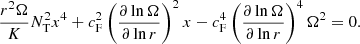 (K.4)
(K.4)
with x = (ωA/Ω)2.
The magnetic model is based on the Tayler-Spruit (TS) dynamo mechanism (Spruit 2002) with modifications proposed by Eggenberger et al. (2022a) (see Sect. 3.2). Before to describe this modification, let us remind that the TS dynamo starts from the fact that the radial component of a small initial magnetic field will be wound up by differential rotation. Rapidly, the azimuthal component, whose amplitude increases linearly with time, will dominate the radial one and at a given point will become unstable. Since the energy that can be extracted from the magnetic field is small, the first instability that can occur should be one minimizing the energy. Any radial instability has to overcome the stabilizing effects of the entropy gradient in a radiative zone, thus the most favorable instabilities are mainly developing horizontally (this is a bit the same idea at the origin of the Dh in the theory by Zahn 1992 although, here the instability has its origin in an instability of the magnetic field not linked to the horizontal differential rotation). Tayler (1973), Pitts & Tayler (1985) have shown that a weak azimuthal field is unstable along a kink and pinch type instability as soon as some conditions are met. This generates a new small radial field that will be wound up, generating an azimuthal field that will be become unstable. The dynamo loop is closed.
In those magnetic models the main driver for the transport of the angular momentum is the magnetic viscosity. The main driver for the transport of the chemical elements are the meridional currents. The diffusion coefficient (that mixes the chemical species) describing the Tayler instability is too small for having a significant effect.
As explained above, an expression for the magnetic viscosity ν and for the magnetic diffusivity, η, are needed. Since the viscosity is associated to the Lorentz force, an important quantity to obtain is the magnetic field (or equivalently the Alven frequency  ) that is reached when the magnetic amplification timescale is equal to the damping one. The amplification timescale, defined as the time needed to amplify the radial magnetic field to an azimuthal magnetic field whose amplitude would be equal to the already existing one is given by (Spruit 2002; Fuller et al. 2019; Eggenberger et al. 2022a)
 (K.5)
(K.5)
where 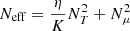 and where we have used that
  and Br = BΦωA/Neff. The damping timescale is taken as
 (K.6)
(K.6)
where Eggenberger et al. (2022a) introduced the factor CT to account for the uncertainties pertaining this damping timescale (CT corresponds to the parameter α3 in Fuller et al. 2019). Equating these two timescales allows to obtain a relation between the magnetic field B (actually here BΦ which is much larger than Br) and η the magnetic diffusion coefficient
 (K.7)
(K.7)
.
This above equation has two unknowns, ωA and η. Thus, we need a second equation to resolve the system. The second equation is obtained by two conditions on the lengthscale of the domain where the instability develops. This lengthscale should be large enough for not being quickly damped by magnetic diffusion and small enough for allowing the excess energy in the shear to allow to overcome the stabilizing entropy gradient. When these two lengths are assumed to be equal, it means that we are just at the limit of the instability to be triggered (namely the excess of energy in the differential rotation just allow to displace the matter over a length that corresponds to the length over which the magnetic field diffuses. Thus we are just at the limit). Following this, one obtains the equation below just at the limit
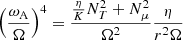 (K.8)
(K.8)
Resolving these two equations give values for ωA (or BΦ) and η.
We can explicit the condition on the shear for the instability to be triggered. The shear q should be larger than a minimum value qmin where qmin is
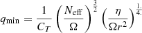 (K.9)
(K.9)
in which η, the diffusion coefficient appears.
The magnetic diffusion coefficient is in absence of any instability the ohmic diffusion coefficient. This diffusivity comes from the fact that magnetic fields are produced by electrical currents that encounters some resistivity in the medium, thus transforming part of the energy into thermal ones. The expression for ohmic diffusion involves a description of how an electron can be deflected by charge along its path. This scatter not only modifies the current and hence the magnetic field but also induce some mixing of elements.
This diffusion is active even if the condition for the instability to be triggered is not fullfilled. As we shall see however this diffusion coefficient is very small. When the condition for the instability is realized (using in qmin for η the value valid in absence of any instability), a new value of η has to be computed. It is obtained resolving the system of two equations above. It is easy to show that replacing the expression of ωA obtained from Eq. NN into Eq. NN, one obtain a fourth order equation that can be written:
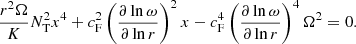 (K.10)
with x = (ωA/Ω)2. The viscosity is then obtained using the same formula as in Spruit (2002)
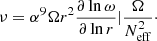 (K.11)
Let us note that η and ν are used in the whole radiative region.
In the magnetic models, we also account for two other hydrodynamical instability, the one linked to shear (both in the vertical and horizontal direction) and the one associated with the meridional currents. In the present magnetic models, we chose the expression of Dshear given by Maeder (1997) and the value of Dh by Maeder (2003). In the present paper, we did not explore the impact of different choices for these quantities in the magnetic models. For the transport of the chemical specied, we have therefore that the total diffusion coefficient appearing in Eq. NN is equal to blabla. For the transport of the angular momentum, we considered only the purely diffusive part of the transport equation. Actually the transport by advection is neglected in these models. We remind that the transport of the angular momentum is clearly dominated by the magnetic coupling and thus this should not affect much the results to neglect the effect of the meridional currents. We note also that would the transport by meridional currents be described by a diffusive equation, it would artificially impose a transport in a direction that is in the wrong direction with respect to what it should be be!
Appendix L: The present numerical experiments compared to other works
The grids of non-magnetic stellar models published so far by our group have used for Dshear the expression by Maeder (1997) and the value of Dh given by Zahn (1992). Thus to take the labels given in Table 1, the grids are using the prescritions of models A.
The magnetic models presented in the present work differs from those discussed in paper III in many respect. We always used the value of η given by the resolution of the fourth order equation.
Compared to the approach used by the rotating models published so far with MESA, the present approach is different in the following respect:
-
when the meridional currents dominate the angular momentum transport, they are accounted for resolving an advective equation and not a diffusive one as in MESA.
-
We do not not use parameters like fC and fμ.
All Tables
All Figures
|
Fig. 1. Internal profiles of K, the thermal diffusivity, Dconv, the convective diffusion coefficient, Dshear, the shear diffusion coefficient, Dh, the horizontal turbulence coefficient, and Deff, the effective diffusivity in 15 M⊙ models at solar metallicity. Each panel is labeled with a letter corresponding to the first column of Table 1. The profile is taken when the central mass fraction of hydrogen Xc = 0.35. |
| In the text | |
|
Fig. 2. Evolution of various physical parameters of the 15 M⊙ models. Left panel: evolutionary tracks during the MS phase in the Hertzsprung-Russell diagram of the 15 M⊙ at Z = 0.014 and with Vini/Vcrit = 0.4. The letters A to G correspond to the models described in Table 1. Center panel: variation in the mass fraction of hydrogen as a function of the Lagrangian mass coordinate when the central mass fraction of hydrogen is 0.35 (Xc = 0.35). Right panel: evolution of the angular velocity vs. the internal mass coordinate at Xc = 0.35 through hydrogen burning. |
| In the text | |
|
Fig. 3. Central and surface properties of 15 M⊙ models. Left panel: mass of the convective core in solar mass as a function of the central mass fraction of hydrogen Xc in different 15 M⊙ models. Right panel: evolution of the surface abundance ratio N/H (normalized to its initial value and in logarithmic scale) as a function of log gsurf for the same models as presented in the left panel. In both panels, the letters have the same meaning as in Fig. 2. |
| In the text | |
|
Fig. 4. Change is physical parameters of M⊙ models with respect to changing helium fractions. Left panel: evolution of the effective temperature as a function of the central helium abundance for different 15 M⊙ models. Right panel: helium profile vs. the mass in different 15 M⊙ models when the central helium mass fraction is 0.90. In both panels, the letters have the same meaning as in Fig. 2. |
| In the text | |
|
Fig. 5. Angular velocity profiles as a function of mass for different 15 M⊙ models at various evolutionary stages. The letters have the same meaning as in Fig. 1. |
| In the text | |
|
Fig. 6. Variation as a function of the radius of K, the thermal diffusivity, Dconv, the convective diffusion coefficient, Dshear, the shear diffusion coefficient, Dh, the horizontal turbulence coefficient, and Deff, the effective diffusivity in different 60 M⊙ models at solar metallicity. The letters correspond to models computed with the prescription given in the second column of Table 1. The profiles are taken when the central mass fraction of hydrogen Xc = 0.35. |
| In the text | |
|
Fig. 7. Evolution of physical parameters of 60 M⊙ models. Left panel: evolutionary tracks in the Hertzsprung-Russell diagram. Center panel: abundance of hydrogen ranging from the center to the outer envelope of the models at Xc = 0.35 vs. the Lagrangian mass coordinate and (right panel) the variation in angular velocity as a function of the Lagrangian mass coordinate in 60 M⊙ at Z = 0.014 and with Vini/Vcrit = 0.4. The letters A to G correspond to the models as described in Table 1. |
| In the text | |
|
Fig. 8. Evolutionary tracks in the Hertzsprung-Russell diagram (left panel), variation in the convective core mass vs. the central mass fraction of hydrogen (center panel), and the surface abundances of hydrogen, helium, carbon, nitrogen, and oxygen against the mass for models C and C*, as described in Table 1. |
| In the text | |
|
Fig. 9. Variation in the angular velocity profiles as a function of mass for 60 M⊙ for models A to D and C* from left to right (see Table 1). |
| In the text | |
|
Fig. 10. Mixing coefficients and their impact in 15 M⊙ models. Left panel: internal profiles of K, the thermal diffusivity, Dconv, the convective diffusion coefficient, Dshear, the shear diffusion coefficient, Dh, the horizontal turbulence coefficient, and Deff, the effective diffusivity in the 15 M⊙ C* model with internal magnetic fields at solar metallicity. The quantities are plotted when the central mass fraction of hydrogen Xc = 0.35. Middle panel: variation in the H-mass fraction vs. the Lagrangian mass coordinate. Right panel: variation in the angular velocity vs. mass in 15 M⊙ for the C* and C models at the end of H burning. |
| In the text | |
|
Fig. 11. Models C and C* with a mass 15 M⊙ with Vini/Vcrit = 0.4. Left panel: evolutionary tracks in the Hertzsprung-Russell diagram during the MS phase. Middle panel: change in the nitrogen to hydrogen ratio normalized to the initial value vs. the surface gravity. Right panel: variation in the effective temperature as a function of the central helium mass fraction. |
| In the text | |
|
Fig. 12. Evolution of the B/H ratio (in number) at the surface of models A (continuous black curve), B (dashed green curve), C (dashed red curve), D (dotted blue curve), and C* (continuous magenta curve) models as a function of the surface gravity. |
| In the text | |
|
Fig. 13. Variation in the angular velocity as a function of the Lagrangian mass coordinate in 15 M⊙ at different evolutionary stages. The left panel shows the nonmagnetic model C. The right panel shows the magnetic model C*. |
| In the text | |
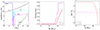 |
Fig. 14. Same as Fig. 10 for 60 M⊙ models. |
| In the text | |
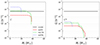 |
Fig. 15. Same as Fig. 13 for 60 M⊙ models. |
| In the text | |
|
Fig. C.1. HR diagram for four (Ledoux and Schwarzschild, long and short timescales) 15 M⊙ models without rotation, showing a comparison of the effect of the time resolution on evolution. |
| In the text | |
|
Fig. E.1. Variation of physical parameters in the 15 M⊙ models. Left panel: Evolutionary tracks during the MS phase in the Hertzsprung-Russell diagram for models C, D, E, and F (see Table 1) as a function of the Lagrangian mass for the 15 M⊙ at Z = 0.014 and with Vini/Vcrit = 0.4. Middle panel: Abundance of hydrogen in mass fraction ranging from the center to the outer envelope of the models when the central mass fraction of hydrogen is Xc = 0.35. Right panel: Variations in the angular velocity vs. the mass coordinate for the same models as are shown in the middle panel. |
| In the text | |
|
Fig. E.2. Additional physical parameters during the evolution of various 15 M⊙ models. Left panel: Evolution of the convective core mass during the MS phase as a function of central mass of hydrogen. Center panel: Abundance ratio of nitrogen and hydrogen at the surface normalized to their initial values vs. the surface gravity. Right panel: Profile of the helium mass fraction against the mass coordinate when the central helium fraction Yc is 0.90. The letters C to F correspond to the models with different prescriptions as described in Table 1. |
| In the text | |
|
Fig. E.3. Evolution of the effective temperature as a function of the mass fraction of helium at the center during the core He-burning phase for models C, D, E, and F. |
| In the text | |
Current usage metrics show cumulative count of Article Views (full-text article views including HTML views, PDF and ePub downloads, according to the available data) and Abstracts Views on Vision4Press platform.
Data correspond to usage on the plateform after 2015. The current usage metrics is available 48-96 hours after online publication and is updated daily on week days.
Initial download of the metrics may take a while.