| Issue |
A&A
Volume 700, August 2025
|
|
|---|---|---|
| Article Number | A4 | |
| Number of page(s) | 17 | |
| Section | Planets, planetary systems, and small bodies | |
| DOI | https://doi.org/10.1051/0004-6361/202554766 | |
| Published online | 28 July 2025 | |
Orbit and atmosphere of HIP 99770 b through the eyes of VLTI/GRAVITY
1
European Southern Observatory,
Karl-Schwarzschild-Straße 2,
85748
Garching,
Germany
2
LIRA, Observatoire de Paris, Université PSL, CNRS, Sorbonne Université, Université de Paris,
5 place Jules Janssen,
92195
Meudon,
France
3
Institute of Astronomy, University of Cambridge,
Madingley Road,
Cambridge
CB3 0HA,
UK
4
Leiden Observatory, Leiden University,
PO Box 9513,
2300
RA Leiden,
The Netherlands
5
Department of Physics & Astronomy, Johns Hopkins University,
3400 N. Charles Street,
Baltimore,
MD
21218,
USA
6
Space Telescope Science Institute,
3700 San Martin Drive,
Baltimore,
MD
21218,
USA
7
Division of Space Research & Planetary Sciences, Physics Institute, University of Bern,
Gesellschaftsstr. 6,
3012
Bern,
Switzerland
8
Max Planck Institute for Astronomy,
Königstuhl 17,
69117
Heidelberg,
Germany
9
Fakultät für Physik, Universität Duisburg-Essen, Lotharstraße 1, 47057 Duisburg, Germany Universidade de Lisboa - Faculdade de Ciências, Campo Grande,
1749-016
Lisboa,
Portugal
10
CENTRA - Centro de Astrofísica e Gravitaçâo, IST, Universidade de Lisboa,
1049-001
Lisboa,
Portugal
11
Univ. Grenoble Alpes, CNRS, IPAG,
38000
Grenoble,
France
12
Center for Interdisciplinary Exploration and Research in Astrophysics (CIERA) and Department of Physics and Astronomy, Northwestern University,
Evanston,
IL
60208,
USA
13
Max Planck Institute for extraterrestrial Physics,
Giessenbach-straße 1,
85748
Garching,
Germany
14
Aix Marseille Univ, CNRS, CNES, LAM,
Marseille,
France
15
Université Côte d’Azur, Observatoire de la Côte d’Azur, CNRS, Laboratoire Lagrange,
France
16
STAR Institute, Université de Liège,
Allée du Six Août 19c,
4000
Liège,
Belgium
17
Department of Astrophysical & Planetary Sciences, JILA,
Duane Physics Bldg., 2000 Colorado Ave, University of Colorado,
Boulder,
CO
80309,
USA
18
Institute of Physics, University of Cologne,
Zülpicher Straße 77,
50937
Cologne,
Germany
19
Max Planck Institute for Radio Astronomy,
Auf dem Hügel 69,
53121
Bonn,
Germany
20
Universidade do Porto, Faculdade de Engenharia, Rua Dr. Roberto Frias,
4200-465
Porto,
Portugal
21
School of Physics, University College Dublin,
Belfield,
Dublin 4,
Ireland
22
Astrophysics Group, Department of Physics & Astronomy, University of Exeter,
Stocker Road,
Exeter EX4 4QL,
UK
23
Departments of Physics and Astronomy, Le Conte Hall, University of California,
Berkeley,
CA
94720,
USA
24
European Southern Observatory,
Casilla
19001,
Santiago 19,
Chile
25
Advanced Concepts Team, European Space Agency, TEC-SF, ESTEC,
Keplerlaan 1,
NL-2201,
AZ Noordwijk,
The Netherlands
26
University of Exeter,
Physics Building, Stocker Road,
Exeter
EX4 4QL,
UK
27
French-Chilean Laboratory for Astronomy,
IRL 3386, CNRS and U. de Chile, Casilla 36-D,
Santiago,
Chile
28
Center for Space and Habitability, University of Bern,
Gesellschaftsstr. 6,
3012
Bern,
Switzerland
29
Academia Sinica, Institute of Astronomy and Astrophysics,
11F Astronomy-Mathematics Building, NTU/AS campus, No. 1, Section 4, Roosevelt Rd.,
Taipei
10617,
Taiwan
30
European Space Agency (ESA), ESA Office, Space Telescope Science Institute,
3700 San Martin Drive,
Baltimore,
MD
21218,
USA
31
Department of Earth & Planetary Sciences, Johns Hopkins University,
Baltimore,
MD,
USA
32
Kavli Institute for Astronomy and Astrophysics, Peking University,
Beijing
100871,
PR China
33
Max Planck Institute for Astrophysics,
Karl-Schwarzschild-Str. 1,
85741
Garching,
Germany
34
Excellence Cluster ORIGINS,
Boltzmannstraße 2,
85748
Garching bei München,
Germany
★ Corresponding author.
Received:
26
March
2025
Accepted:
19
June
2025
Abstract
Context. Inferring the likely formation channel of giant exoplanets and brown dwarf companions from orbital and atmospheric observables remains a formidable challenge. Further and more precise directly measured dynamical masses of these companions are required to inform and gauge formation, evolutionary, and atmospheric models. We present an updated study of the recently discovered companion to HIP 99770 based on observations conducted with the near-infrared interferometer VLTI/GRAVITY.
Aims. Through renewed orbital and spectral analyses based on the GRAVITY data, we characterise HIP 99770 b to better constrain its orbit, dynamical mass, and atmospheric properties, as well as to shed light on its likely formation channel.
Methods. Upon inclusion of the new high-precision astrometry epoch, we ran an orbit fit to further constrain the dynamical mass of the companion and the orbit solution. We also analysed the GRAVITY K-band spectrum, placing it into context with literature data, and extracting magnitude, age, spectral type, bulk properties and atmospheric characteristics of HIP 99770 b.
Results. We detected the companion at a radial separation of 417 mas from its host. The new orbit fit yields a dynamical mass of 17−5+6 MJup and an eccentricity of 0.31−0.12+0.06. We also find that additional relative astrometry epochs in the future will not enable further constraints on the dynamical mass due to the dominating relative uncertainty on the Hipparcos-Gaia proper motion anomaly that is used in the orbit-fitting routine. The publication of Gaia DR4 will likely ease this predicament. Based on the spectral analysis, we find that the companion is consistent with spectral type L8 and exhibits a potential metal enrichment in its atmosphere. Adopting the AMES-DUSTY model to infer its age, within its dynamical mass constraint the companion conceivably corresponds to either a younger (28−14+15 Myr) object with a mass just below the deuterium-burning limit or an older (119−10+37 Myr) body with a mass just above the deuterium-burning limit.
Conclusions. These results do not yet allow for a definite inference of the companion’s formation channel. Nevertheless, the new constraints on its bulk properties and the additional GRAVITY spectrum presented here will aid future efforts to determine the formation history of HIP 99770 b.
Key words: techniques: interferometric / techniques: spectroscopic / planets and satellites: atmospheres / planets and satellites: formation / planets and satellites: gaseous planets
© The Authors 2025
 Open Access article, published by EDP Sciences, under the terms of the Creative Commons Attribution License (https://creativecommons.org/licenses/by/4.0), which permits unrestricted use, distribution, and reproduction in any medium, provided the original work is properly cited.
This article is published in open access under the Subscribe to Open model. This email address is being protected from spambots. You need JavaScript enabled to view it. to support open access publication.
1 Introduction
Gas giant exoplanets that are accessible to direct-imaging studies are rare. Unbiased blind surveys have provided only a few detections (e.g. Nielsen et al. 2019; Vigan et al. 2021; Chomez et al. 2025; for a review, see Bowler 2016) and demonstrated that targeted studies, for instance informed by clues stemming from other detection techniques such as astrometric monitoring of potential host stars, are the only way to efficiently build a population-level sample of directly imaged exoplanets.
The source HIP 99770 was identified as exhibiting a significant proper motion anomaly (PMa; see Kervella et al. 2022; Brandt 2021), the discrepancy between the proper motion of a star as observed by the Hipparcos (Schuyer 1985) and Gaia missions (Gaia Collaboration 2016). Such a PMa can be caused by an orbiting companion inducing reflex motion in the star that manifests itself in its projected movement on the sky plane, and thus, in its proper motion. A dedicated direct-imaging followup using SCExAO/CHARIS (Jovanovic et al. 2015; Groff et al. 2017) on the Subaru Telescope and Keck/NIRC2 revealed a substellar companion with a dynamical mass of  (Currie et al. 2023). Hence, HIP 99770 was the first system to yield a detection of a companion identified as a planet after it was targeted specifically on the basis of tentative astrometric evidence that indicated the existence of an orbiting object. The loose mass constraint places the companion in close proximity to the deuterium-burning threshold, implying a need for further observations to pin down its mass1.
The necessity of follow-up studies of this object becomes all the more apparent when we consider the relative scarcity of what are loosely referred to as super-Jupiters (Carson et al. 2013), that is, substellar companions with masses at about the deuterium-burning threshold. These objects tend to defy the commonly proposed planet formation mechanisms. On the one hand, the disc-instability pathway, which posits that planets form via the gravitational collapse of the circumstellar disc (Cameron 1978; Boss 1997; Kratter & Lodato 2016), is predicted to form more massive companions well within the brown dwarf or even stellar mass regime (Forgan & Rice 2013). On the other hand, formation via core accretion in the outer disc is difficult to justify because the required timescales at these distances from the host are significantly longer than the typical disc-dissipation timescale (Lambrechts & Johansen 2012). The different pathways are expected to leave telltale imprints on the orbital geometry of the system implying that precisely constraining the orbital elements of a given companion can reveal clues as to its formation history (e.g. Bitsch et al. 2020; Marleau et al. 2019). Given its long period orbit (approximately 50 years; Currie et al. 2023) and its recent discovery based on data collected between 2020 and 2021, the current orbit coverage of HIP 99770 b is limited. An extension of the available astrometric baseline will help us improve the orbital solution.
An alternative and complementary route towards probing the formation history of a given companion is the characterisation of its atmosphere. Observables such as the atmospheric metal-licity or elemental abundance ratios, which are accessible via a spectroscopic analysis of the flux emitted by the companion, can add to the conclusions drawn from orbital considerations (e.g. Mollière et al. 2022). For the specific case of HIP 99770 b, a recent high-resolution spectroscopic follow-up yielded constraints on the metallicity and elemental abundance ratios of the companion (Zhang et al. 2024). These were unable to exclude either formation pathway, however. In addition to these continuum-removed high-resolution K-band spectra, a new data set that preserves the continuum emission component of the companion (albeit at a lower resolution) can shed new light on the atmospheric properties of the companion.
Here, we present new VLTI/GRAVITY (GRAVITY Collaboration 2017) observations of HIP 99770 b, describe how they facilitate constraints on the orbital geometry of the system and act as yet another window into the companion atmosphere. GRAVITY is a near-infrared interferometric instrument at the European Southern Observatory’s Very Large Telescope (VLT). Previous studies using the instrument for exoplanet observations have demonstrated an astrometric accuracy of 50 μas (GRAVITY Collaboration 2019).
This paper is arranged as follows: Section 2 gives an overview of the observational data we used. The orbital and spectral analyses of the obtained data are presented and discussed in Sects. 3 and 4, respectively. The conclusions of our study are laid out in Sect. 5.
2 Observations and data reduction
2.1 Previous observations
This work draws upon data that were collected by previous studies of the HIP 99770 system. We used the astrometric epochs and the photometric and spectral data obtained by Currie et al. (2023). The CHARIS spectrum contained therein consists of 22 channels covering the wavelength range between 1.16 and 2.37 μm at a resolution of approximately 20. Additionally, the orbital fit performed in Sect. 3 is partially based on the host star absolute astrometry as listed in the Hipparcos-Gaia Catalogue of Accelerations (HGCA; Brandt 2021).
2.2 VLTI/GRAVITY
We observed HIP 99770 b with the GRAVITY instrument on 31 May and 2 July 2023. These observations were obtained on technical time and in the framework of the ExoGRAVITY Large programme (ESO ID 1104.C-0651, Lacour et al. 2020). An observation log for both epochs can be found in Table 1. Notably, they were taken using different observing modes. For the first epoch, we used the dual-field on-axis mode, while the second epoch was obtained in dual-field off-axis mode. Importantly, the latter mode enables a higher signal-to-noise ratio (S/N) because the entire light of the sources that is collected by the four unit telescopes is injected into the fringe tracker and science fibre channels by means of a rooftop mirror. This is not the case for on-axis observations, where a beam splitter directs only half the light into the different channels. A comprehensive comparison of the two observing modes is given by Nowak et al. (2024). For both observations, the placement of the science fibre was informed by orbital fits applied to the available direct detections of the companion (see Sect. 2.1 and Table 2).
We used the ESO GRAVITY instrument pipeline 1.6.4b1 for the data reduction. This yielded the so-called “astroreduced” byproduct, from which the relative astrometry between host and companion can be extracted following the standard exoplanet dual-field data processing outlined in Appendix A of GRAVITY Collaboration (2020). The first detection on 31 May 2023 is visualised in Fig. 1, the resulting relative astrometry epoch is listed in Table 2. Because the off-axis observation mode was employed for the second epoch, the collected data necessitated a special reduction procedure. To measure the metrology zero point, we performed a swap observation of a calibration binary, which in this case was HD 196885 AB. The binary observation was based on a poor relative position prediction, and the pointing of the single-mode fibres was therefore off by approximately 35 mas. The field aberrations resulting from this pointing deviation (GRAVITY Collaboration 2021) caused a bias in the zero-point estimate of up to 30 degrees. As a consequence, the astrometric measurement of the science target HIP 99770 b was uncertain, which caused us to discard this astrometric epoch from our orbital analysis.
For each epoch, we also obtained a K-band companion-to-host contrast spectrum ranging from 1.97 to 2.48 μm at a resolution of R = 500. Depending on the angular distance between the astrometric position of the companion and the centre of the science fibre, we needed to correct the spectra for throughput losses. A detailed description of how this is accounted for is provided in Appendix C. To convert the companion contrast spectra measured by GRAVITY into companion flux spectra that could be used for the atmospheric analysis and modelling, we first multiplied them with the flux spectrum of the amplitude reference source, that is, the host star HIP 99770 A for the on-axis, and the binary (swap) calibrator HD 196885 AB for the off-axis epoch. To obtain model spectra of these targets, we fitted a BT-NextGen and a BT-Settl (CIFIST) solar metallicity stellar model atmosphere (Allard et al. 2012) to archival photometric data from Gaia and Tycho using the species toolkit (Stolker et al. 2020). Additionally, we included the Gaia XP spectrum of HIP 99770 A and HD 196885 AB in these fits. When we also incorporated 2MASS photometry, the inferred stellar model parameters did not change by more than 1 σ. Based on PyMultiNest (Feroz & Hobson 2008; Feroz et al. 2009; Buchner et al. 2014), the nested-sampling approach implemented within species enables the inference of the posterior distributions of the individual model parameters. Following Cardelli et al. (1989), we also accounted for extinction by the interstellar medium that might affect HIP 99770 A by setting the V-band extinction parameter, AV, to 0.043 mag (Murphy & Paunzen 2017). To further guide the spectral fits to physically plausible solutions, we invoked Gaussian priors on the mass of HIP99770A of M = 1.8 ± 0.2 M (Currie et al. 2023) and on the effective temperatures and masses of the two binary components of HD 196885 AB using the values and uncertainties reported in Table 1 of Chauvin et al. (2023) (Teff,A = 6340 ± 19 K, Teff,B = 3660 ± 190 K, MA = 1.3 ±0.1 M⊙, MB = 0.45 ± 0.01 M). We converted the M1±1 spectral type constraint of component B that is reported in this table into an effective temperature constraint using Table 5 of Pecaut & Mamajek (2013). For more details on the conversion of contrast to flux, we refer to Appendix D. The mass and effective temperature values of HIP 99770 A inferred from our fit are within 2σ of the value reported by Murphy & Paunzen (2017), those of HD 196885 AB are within 3σ of the values reported by Chauvin et al. (2023).
The resulting on- and off-axis flux spectra normalised by the respective amplitude references are significantly offset relative to each other. Since the off-axis reference (swap) binary HD 196885 AB was observed with a significant mispointing of the fibre, a lower throughput is expected (estimated at −45% in Table 1). This biased our photometric calibration. The on-axis observations of HIP 99770 b, on the other hand, were calibrated quasi-simultaneously as a result of the continuous monitoring of the host star spectrum, with GRAVITY science spectrometer observations interspersed between the planet observations. The on-axis spectrum is therefore more reliable, and we opted for scaling the off-axis companion flux spectrum such that it matched the on-axis spectrum best. The best-fitting scale factor was found to be 61%.
Finally, we combined the companion flux spectra for the two epochs into a single covariance-weighted mean spectrum that we used for the analysis presented in Sect. 4. The spectral reduction process is visualised in Fig. 2. This is the first time a GRAVITY exoplanet off-axis spectrum without an on-axis amplitude reference is published.
GRAVITY observation log of the target HIP 99770 b and of the swap calibrator HD 196885 AB.
Astrometric detections of HIP 99770 b.
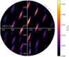 |
Fig. 1 Detection of HIP 99770 b on 31 May 2023. The circular panel indicates the field of view of the GRAVITY science fibre. The map within visualises the |


3 Orbital analysis
To obtain constraints on the companion mass and orbital parameters, we performed an orbit fit of the relative astrometry epochs presented in Table 2 using the orbitize! package (Blunt et al. 2020). Its MCMC sampling routine allowed us to include the absolute astrometry of the host star collected by the Hippar-cos and Gaia missions (conveniently presented by Brandt 2021). The orbitize! sampling procedure is an implementation of ptemcee (Vousden et al. 2016), a parallel-tempered affine-invariant Markov chain Monte Carlo (MCMC) algorithm based on emcee (Foreman-Mackey et al. 2013). It was carried out using 20 temperatures and 100 walkers taking 4 × 10⁴ burn-in steps and another 4 × 10⁴ actual sampling steps each. These walkers were let loose on nine free parameters, namely the semi-major axis, a, the eccentricity, e, the inclination, i, the argument of periastron, ω, the longitude of the ascending node, Ω, the relative epoch of periastron2, τ, the parallax, π, the stellar mass, Mhost, and the companion mass, Mcomp. The priors we chose for the individual free parameters are listed in Table 3. We carried out two separate sampling runs. The first run was performed using the Hipparcos-Gaia stellar astrometry and the previous astrometric companion detections (Currie et al. 2023) only. We then resampled the posterior distributions upon inclusion of our own GRAVITY detection from 31 May 2023. With the two resulting posterior samplings in hand we investigated how the addition of a GRAVITY detection changed the inferred parameter values and their uncertainties. By means of visual inspection of the chain traces for the individual parameters, we confirmed that the walker chains converged for all parameters and for both runs. The two posterior samplings of the orbital parameters are shown in Fig. 4. A random subset of the posterior sampling was used to visualise the projection of the companion orbit onto the sky plane in Fig. 3.
The bottom right panel of Fig. 4 shows that the resampling procedure resulted in a slightly increased companion mass of  3.
3.
To investigate the extent to which this result is driven by the uniform companion mass prior, we ran an additional sampling procedure using a log-uniform prior distribution instead. This yielded a lower posterior mass of  3, a behaviour consistent with the findings by Currie et al. (2023). Along the same lines, we examined the dependence of the inferred companion mass on the stellar mass prior. Retaining the standard deviation of 0.2 M, we performed further posterior samplings based on underlying Gaussian priors that were shifted from the original 1.8 to 1.7 in the first and 1.9 M in the second run. These modifications resulted in a companion mass of 1
 3 (decrease of 12%) and
  3 (increase of 0.5%), respectively. A comparison between the resulting posterior mass distributions is shown in the top right panel of Fig. A.1. Since these adjustments to the shapes and positions of the priors affect larger posterior displacements than the inclusion of the GRAVITY astrometry epoch, the slight shift in companion mass evident in Fig. 4 does not necessarily amount to a robust inference of a higher dynamical mass.
The manifest inability to further constrain the companion mass comes as somewhat of a surprise given the high angular resolution of the new GRAVITY astrometry epoch. It is, however, not driven by the individual astrometric epochs or the amount thereof, but by the large relative uncertainty of the Gaia-Hipparcos PMa. Following Kervella et al. (2019), we computed the PMa as the difference between the Gaia DR3 proper motion vector, μG3, and the long-term Hipparcos-Gaia DR3 proper motion vector, μHG3, which both consist of a right ascension and declination component. Carrying the respective uncertainties, we found the PMa to be

where all components are given in units mas/yr, and the proper motion values were taken from Brandt (2021). Thus, the relative uncertainties on the RA and Dec components are approximately 80 and 51%, respectively. This large PMa uncertainty dominates so thoroughly that even additional GRAVITY epochs in the future would not help constrain the companion mass further. Tighter error bars on the mass can therefore only be obtained once a more precise PMa will be available in Gaia DR4. To substantiate this finding, we performed several orbital resampling runs including varying numbers of mock GRAVITY epochs predicted from the current best fit. While these additional artificial epochs served to narrow down the posterior distributions of the remaining orbital parameters, they likewise fail to further constrain the companion mass. For instance, when we iteratively generated an additional three GRAVITY astrometric mock epochs based on the newly obtained orbit solution, we found an improvement of approximately 1% in relative uncertainty of the companion semi-major axis, but no such gain is achieved in the precision of its mass.
While the addition of the GRAVITY astrometry epoch yielded no improved constraints on the companion mass, it did pin down the orbital semi-major axis at  and the eccentricity at
  . The strong constraint on the orbital eccentricity is a marked improvement on the previously available solution. While a circular orbit was conceivable prior to the GRAVITY detection (Currie et al. 2023), this configuration is now decisively ruled out. HIP 99770 b therefore joins a growing number of substellar companions exhibiting elevated eccentricities. Examples of other recently detected eccentric companions are 51 Eri b (Macintosh et al. 2015) with
  (Dupuy et al. 2022) and Eps Ind A b (Feng et al. 2019) with
  (Matthews et al. 2024).
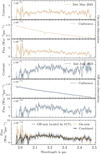 |
Fig. 2 Ingredients and outcome of the spectral data reduction. The top three panels show the GRAVITY on-axis contrast spectrum, the associated stellar calibration flux spectrum, and the resulting companion flux spectrum. The same is visualised for the off-axis observation in the three middle panels. Finally, the bottom panel shows the on- and off-axis companion flux spectra alongside the combination of the two. This K-band spectrum of HIP 99770 b is used in Sect. 4. |
Orbital parameter priors and posteriors.
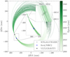 |
Fig. 3 Orbit of HIP 99770 b relative to its host, i.e., fixed at the origin. The visualised orbits were generated from a random subset of 100 parameter sets drawn from the posterior sampling. While the previously available astrometric epochs obtained by SCExAO/CHARIS and Keck/NIRC2 are shown along with their respective uncertainties in ΔRA and ΔDec, knowledge of the correlation coefficient, ρ, allowed us to visualise the VLTI/GRAVITY epoch as a 1 σ confidence ellipse. |
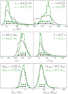 |
Fig. 4 Marginalised posterior distributions of a subset of the fitted orbital parameters. The black posteriors were sampled considering the previously available data only, while the green posteriors result from the inclusion of the new GRAVITY epoch from 31 May 2023. The median values and intervals between the 16th and 84th percentiles of the distribution are indicated by the horizontal bars. The inferred values resulting from the two runs, which were rounded to the respective significant figure, are displayed at the top of each panel. While technically not one of the parameters explored by the walkers during the sampling procedure, we also plot the period, P, as computed from the other posteriors via Kepler’s third law. The full posterior samplings can be found in Appendix A. |
4 Spectral analysis
4.1 Spectral classification
We folded the GRAVITY K-band spectrum with the Paranal/SPHERE.IRDIS_B_Ks, IRDIS_D_K12_1, and IRDIS_D_K12_2 filter profiles to position HIP 99770 b in a colour-magnitude diagram (CMD) and thereby place it in the context of a literature population of companion and free-floating brown dwarfs and exoplanets. This folding procedure yielded absolute companion magnitudes of MKs = (12.460 ± 0.014) mag, MK2 = (12.34 ± 0.02) mag, and MK1 = (12.56 ± 0.02) mag. The resulting CMD is shown in Fig. 5 and indicates that HIP 99770 b is compatible with a late L- to early T-type object. We also folded the GRAVITY spectrum with the MKO/NSFCam.Ks filter profile and obtained an absolute magnitude of (12.544 ± 0.013), which lies within the 68% confidence interval of the discovery paper measurement of (12.61 ± 0.09) (Currie et al. 2023).
To achieve a more quantitative classification, we used the empirical spectral type fitting routine implemented in species. Based on minimising the goodness-of-fit statistic, Gk (Cushing et al. 2008), this procedure compares the spectrum of a given object to near-infrared reference spectra of low-mass stars, brown dwarfs, and exoplanets within the SpeX Prism Library. We first performed this fit on the composite spectrum, consisting of the GRAVITY and CHARIS spectra. The latter was obtained with the original discovery of the companion (Currie et al. 2023). To ensure that the two spectra were consistent with one another, we computed a GRAVITY scaling factor using the CHARIS spectrum as a calibration baseline. Rebinning the GRAVITY spectrum onto the CHARIS wavelength solution using SpectRes (Carnall 2017) allowed us to directly compare the two spectra in the wavelength region in which they overlap (2.00 to 2.37 μm). We applied a simple scaling factor, α, to the GRAVITY spectrum and subsequently compared it to the CHARIS spectrum by minimising a mutual chi-squared metric. This suggested a scaling factor of α = 0.86 to facilitate the best agreement. Fig. 6 shows that for the composite CHARIS and GRAVITY spectrum, the Gk-minimum is reached at a spectral type of L8. To explore the effect of only having access to a narrower wavelength coverage, we performed another spectral classification run that only considered the higher-resolution GRAVITY spectrum. In addition to preferring the earlier spectral type of L6, the GRAVITY K-band spectrum by itself proved less capable of excluding other, especially earlier spectral types. Whereas in the GRAVITY-only run, these types showed an only minimally higher and thus only marginally less appropriate goodness-of-fit statistic than the L8 bin, they were significantly disfavoured in the composite CHARIS and GRAVITY run. As a consistency check, we repeated the spectral classification using the SpeX Prism Library Analysis Toolkit (SPLAT; Burgasser & Splat Development Team 2017), which likewise yielded L8 for CHARIS and GRAVITY data and L6 for the GRAVITY spectrum alone.
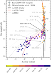 |
Fig. 5 Colour-magnitude diagram showing HIP 99770 b, indicated by the black diamond, in relation to a literature population of low-mass stars, brown dwarfs, and exoplanets (see Appendix C of Bonnefoy et al. 2018 and references therein). All ExoGRAVITY targets (ESO ID 1104.C-0651; Lacour et al. 2020) and the companions so far detected via the Gaia-GRAVITY synergy (Winterhalder et al. 2024) are shown in light blue and ochre, respectively. Additionally, isochrones computed using the AMES-Dusty (Chabrier et al. 2000; Allard et al. 2001), AMES-Cond (Allard et al. 2001; Baraffe et al. 2003), and ATMO (Phillips et al. 2020) evolutionary models are shown for two ages: 1 Gyr (solid lines), and 100 Myr (dotted lines). The filters we used to extract these magnitudes and colours from the spectra are Paranal/SPHERE.IRDIS_B_Ks, IRDIS_D_K12_1, and IRDIS_D_K12_2. |
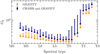 |
Fig. 6 Goodness-of-fit statistic, Gk, (Cushing et al. 2008) as a function of spectral type when comparing the CHARIS and GRAVITY spectra together and the GRAVITY spectrum alone to empirical spectra. The minimum Gk value in each spectral type bin is indicated by the coloured circles, the error bars display the full Gk range resulting from all empirical spectra within the respective bin. |
4.2 Constraining the system age
In Sect. 4.1, the companion was shown to correspond to a late L- to early T-type which implies a cloudy atmosphere. This circumstance needs to be accounted for when selecting an appropriate evolutionary model. As is evident from Fig. 5, based on their physics and cloud prescriptions, the models can vary in their applicability to different objects. While the AMES-Cond (Allard et al. 2001; Baraffe et al. 2003) and ATMO (Phillips et al. 2020) models appear to be poorly suited to describing objects just above the L-T transition, the AMES-Dusty model (Chabrier et al. 2000; Allard et al. 2001) captures the position of HIP 99770 b on the CMD reasonably well. It is thus a suitable model for constraining the system age. To this end, we used the companion Ks-band filter magnitude of (12.460 ± 0.014) mag obtained by folding the GRAVITY K-band spectrum with the IRDIS_B_Ks filter profile. This approach clearly yielded an unrealistically precise magnitude since merely propagating the errors on the flux measurements in each wavelength channel did not take the calibration offset into account that was determined relative to the CHARIS spectrum in Sect. 4.1. Based on the scaling factor α = 0.86, we adopted a systematic error of 14% which (at an IRDIS_B_Ks filter magnitude of 12.46 mag) translates into an error of 0.15 mag.
Figure 7 places this filter magnitude in context with a set of AMES-Dusty grid isochrones in the vicinity of the dynamical mass of the companion. For any given mass-magnitude pair, we can compute the corresponding age as implied by the model by minimising a loss function that compares the measured magnitude to a given AMES-Dusty isochrone magnitude at the mass in question. By thus finding the isochrone that best describes the mass-magnitude pair, we obtained the best-fitting age. We applied this bootstrapping procedure to 106 mass-magnitude pairs drawn from the dynamical mass posterior distribution and a Gaussian IRDIS_B_Ks distribution, N(12.46 mag, 0.15 mag), which takes the dominant systematic calibration error into account. This yielded the age distribution visualised in the small panel in the bottom right corner of Fig. 7.
The bimodal nature of the age distribution is a direct consequence of the circumstance that HIP 99770 b occupies a region in the mass-magnitude plane in which deuterium can affect the cooling of the companion as it ages. The mass-dependent position of the deuterium-burning shoulder in the cooling (luminosity) curves at constant mass as a function of time (e.g. Burrows et al. 2001; Saumon & Marley 2008; see a similar feature in Hinkley et al. 2023) causes a ripple, or a peak4, in the isochrones that is clearly visible in Fig. 7.
Computation of the median and 68% confidence intervals of both modes yielded the two possible age scenarios of  and
and  , where y and o denote younger and older, respectively. The older scenario is strongly preferred in terms of its statistical power. There is also a non-zero probability that the companion occupies a position between the two modes in close proximity to the deuterium shoulder (see also Fig. 8 of Burrows et al. 2001). Using ATMO (Phillips et al. 2020) as the underlying evolutionary model to convert the companion K-band magnitude and dynamical mass into an age, we found similar results. The two modes are located at
  and
and  . Currie et al. (2023) placed the age of this system between 40 and 400 Myr, but emphasised that a self-consistent treatment similar to what we outlined above suggests an age between 115 and 200 Myr, which broadly agrees with our older scenario. More precise knowledge of the companion mass would disambiguate between the two modes of our age distribution. Thus, the main hindrance preventing a firmer age constraint is again the looseness of the dynamical mass constraint.
The above analysis and age constraint hinges on the validity of the evolutionary model for HIP 99770 b. Several aspects warrant caution. Firstly, instances in which evolutionary models deviate from the observed characteristics of exoplanets are well documented, an example being the tensions exhibited by older substellar companions with constrained dynamical masses (e.g. Dupuy et al. 2009; Kuzuhara et al. 2022; Franson et al. 2023a). Secondly, and perhaps more importantly for HIP 99770 b, for young objects, an uncertainty persists as to whether the onset of companion formation is simultaneous or delayed relative to the disc and host formation (e.g. Franson et al. 2023b; Zhang et al. 2023; Balmer et al. 2025). Because especially at young ages, evolutionary models imply strong gradients in the bulk parameters of companions as a function of time, erroneous assumptions regarding the onset of companion formation can result in flawed inferences.
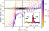 |
Fig. 7 Isochrones from the AMES-Dusty model grid (Chabrier et al. 2000; Allard et al. 2001) in the mass-magnitude plane. The colours indicate the respective age. The solid black lines show the dynamical mass of the companion and the IRDIS_B_Ks filter magnitude, the dotted lines delineate the 16th and 84th percentiles. For the filter magnitude, we adopted a conservative systematic error (see text). The grey colour map in the background visualises the two-dimensional distribution of randomly drawn masses and magnitudes from their respective distributions. The dash-dotted line encircles 68% of all draws. The shoulder in the isochrones in this particular region of the mass-magnitude plane is caused by the onset of deuterium burning and the mass dependence of its time evolution. The panel in the bottom right corner shows the companion age posterior obtained by bootstrapping the drawn mass and magnitude pairs onto the age manifold as defined by the isochrones. |
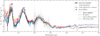 |
Fig. 8 Spectral energy distribution of HIP 99770 b. The black points encircled by a white border and connected by a black line show the CHARIS spectrum taken from Currie et al. (2023). The light grey points depict the combination of the on- and off-axis GRAVITY spectra. For visualisation purposes, a rebinned lower resolution GRAVITY spectrum is shown in dark grey encircled by a white border and connected by a dark grey line. Additionally, the mid-infrared photometry data point in the NIRC2.Lp filter is shown as a black diamond encircled by a white border (Currie et al. 2023). The associated horizontal error bar indicates the FWHM of the filter transmission profile. The spectra resulting from the most likely parameter sets determined by the posterior sampling processes are shown for four different atmospheric forward models. SM Cloudy 2008 denotes the cloudy (fsed = 2) Saumon & Marley (2008) model. |
4.3 Atmospheric forward modelling
Using species, we performed a suite of atmospheric gridmodel fits to the entirety of the spectral and photometric data available for HIP 99770 b. As was the case for the orbit sampling procedure in Sect. 3, every sampling run described below was performed with an underlying Gaussian parallax prior, N(24.55 mas, 0.09 mas), which corresponds to the host parallax angle as listed in Gaia DR3 (Gaia Collaboration 2023). In all fitting procedures, each wavelength channel across both spectra was weighted equally. Additionally, we accounted for correlations between the GRAVITY wavelength channels using the covariance matrix provided by the data reduction pipeline. According to Currie et al. (2023), the covariance matrix associated with the CHARIS spectrum is dominated by spatially and spectrally uncorrelated noise, which likely renders its inclusion insignificant. Similar to the approach outlined in Sect. 4.1, we included an additional factor, α, as a free parameter to allow for a relative flux calibration between the CHARIS and GRAVITY spectra.
Cloudless models such as Sonora Bobcat (Marley et al. 2021) or Saumon & Marley Clear (2008) (Saumon & Marley 2008) did not result in adequate fits. Instead, these models tended to overestimate the spectral energy distribution below 1.9 μm. This was especially the case for the two prominent broad-band spectral features surrounding the water absorption signature at 1.4 μm. The muted nature of these features suggests a cloudy atmosphere. We therefore proceeded to fit the spectral energy distribution using a set of cloudy models. The full corner plots showing the posteriors resulting from sampling linearly interpolated grids of the DRIFT-PHOENIX (Woitke & Helling 2003; Helling & Woitke 2006; Helling et al. 2008), BT-Settl (Allard et al. 2012), Sonora Diamonback (Morley et al. 2024), and Saumon & Marley Cloudy (2008) (Saumon & Marley 2008) models using 1000 live points can be found in Appendix B. As compared to the dynamical mass obtained from the refined orbital solution in Sect. 3, the BT-Settl and Sonora Diamonback models performed poorly in that they inferred significantly lower masses. This is a cause for concern. We therefore conducted an additional posterior sampling run, this time employing a Gaussian companion mass prior, N(17MJup, 6MJup), that reflects the dynamical mass constraint obtained in Sect. 3. The posteriors resulting from this informative mass prior are shown alongside the initial non-informative, that is, uniform, mass prior run in Appendix B. For the problematic models, the inclusion of the informative mass prior was evidently not effective in forcing the walkers to sample a solution within the dynamical mass constraint. Both the Sonora Diamondback and the BT-Settl posterior samplings showed little to no reaction to the application of the informative prior. We conclude that the dynamical mass constraint is too loose to effect a strong and physically accurate pull on the posteriors. Subsequent tests with artificially reduced dynamical mass uncertainties, and thus, stronger, more informative mass priors indeed resulted in the desired forcing confirming that the low current precision of the prior is the cause for its futility. The DRIFT-PHOENIX and Saumon & Marley Cloudy (2008) models, on the other hand, yielded reasonable posterior masses in both the non-informative and informative companion mass prior cases. To assess the performance of the different models and the inferred results on the basis of a consistent set of priors, we only consider the informative mass prior sampling runs hereafter. Figure 8 shows the spectra associated with the most likely parameter sets for each of the chosen models. The median posterior parameter values and 68% confidence intervals are presented in Table 4. The reduced chi-squared values,  , of these best-fitting parameter sets also to be found in Table 4 are acceptable for all models. This quantitatively confirms the qualitative impression that the models manage to capture the overall shape of the spectral energy distribution in Fig. 8. However, the model posteriors in Table 4 and Appendix B reveal that the inferred parameter values can differ significantly between the individual models.
The median effective temperatures of the companion are spread across a range spanning from approximately 1300 to 1770 K with the Sonora Diamondback and DRIFT-PHOENIX models yielding the lowest and highest temperatures, respectively. The surface gravity also varies significantly, with the Sonora Diamondback chain converging on the edge of the prior range at log(g) = 3.6, while DRIFT-PHOENIX places it at approximately 5.0. While BT-Settl and Sonora Diamond-back agree on a radius of approximately 1 RJup, Saumon Marley and DRIFT-PHOENIX converge on 1.5 and 0.6RJup, respectively. The flux scaling factor, α, which is required to reconcile the GRAVITY with the CHARIS spectrum and was derived in Sect. 4.2, is recovered to within 2σ by all fits. Finally, sampling the companion atmosphere metallicity is only supported by the DRIFT-PHOENIX and Sonora Diamondback models. With an inferred metallicity of ![Mathematical equation: $[\mathrm{Fe}/\mathrm{H}]=\SI{0.25(3:6)}{}$](/articles/aa/full_html/2025/08/aa54766-25/aa54766-25-eq50.png) , the chain converges close to the edge of the DRIFT-PHOENIX grid at 0.3. The value agrees well with the somewhat looser
, the chain converges close to the edge of the DRIFT-PHOENIX grid at 0.3. The value agrees well with the somewhat looser ![Mathematical equation: $[\mathrm{Fe}/\mathrm{H}]=\SI{0.27(12:12)}{}$](/articles/aa/full_html/2025/08/aa54766-25/aa54766-25-eq51.png) obtained using the Sonora Diamondback model, however, which is defined over a wider grid that extends to 0.5. Furthermore, they are both consistent with the metallicity measurement of
obtained using the Sonora Diamondback model, however, which is defined over a wider grid that extends to 0.5. Furthermore, they are both consistent with the metallicity measurement of ![Mathematical equation: $[\mathrm{M}/\mathrm{H}]=\SI{0.26(24:23)}{}$](/articles/aa/full_html/2025/08/aa54766-25/aa54766-25-eq52.png) reported by Zhang et al. (2024). An extension of the spectral coverage into the mid-infrared, for instance by means of JWST observations, is likely to further constrain the posteriors, and would thus enable a tighter hold on the companion metallicity and elemental abundance ratios (e.g. see Miles et al. 2023).
reported by Zhang et al. (2024). An extension of the spectral coverage into the mid-infrared, for instance by means of JWST observations, is likely to further constrain the posteriors, and would thus enable a tighter hold on the companion metallicity and elemental abundance ratios (e.g. see Miles et al. 2023).
Following the analysis presented by Nasedkin et al. (2024) and Balmer et al. (2025), we can contextualise this result with other planetary metallicity measurements. To this end, we converted the metallicity relative to the solar value into a metallicity ratio of the companion and the host. There are different metal-licity constraints for HIP 99770 in the literature: Paunzen et al. (1999) placed it at [Fe/H]host = (−1.3 ± 0.2), Paunzen et al. (2002) estimated (−1.46 ± 0.08), while Villaume et al. (2017) inferred −0.8 (no uncertainty reported). These estimates, however, might be superficial since HIP 99770 has been classified as a chemically peculiar λ Boo star (Murphy & Paunzen 2017). Despite the apparent metal depletion suggested by their iron underabundances, these stars are in fact expected to possess bulk solar abundances (e.g. Murphy et al. 2020). Since the companion metallicity inferred using DRIFT-PHOENIX (![Mathematical equation: $[\mathrm{Fe}/\mathrm{H}]_\mathrm{comp}=\SI{0.25(3:6)}{}$](/articles/aa/full_html/2025/08/aa54766-25/aa54766-25-eq53.png) ) is based on a chain that converged towards the edge of the defined grid range, we only considered the estimate obtained using the Sonora Diamondback model (
) is based on a chain that converged towards the edge of the defined grid range, we only considered the estimate obtained using the Sonora Diamondback model ( ). This yielded a metallicity ratio of companion and host of
  which would be consistent with the mass-metallicity relation derived by Thorngren et al. (2016). How these results compare to other companions with measured metallicity ratios as well as the aforementioned empirical relation is visualised in Fig. 9.
The main caveat for assessing the derived metallicity ratios is their dependence on the loosely constrained stellar metal-licity. To illustrate, if we had instead used a host metallicity of [Fe/H]host = (−1.46 ± 0.08), as suggested by Paunzen et al. (2002), the metallicity ratio would have amounted to  , which would indicate strong metal enrichment in the companion. This conclusion might be interpreted in terms of the sequence of formation phases that have led to the current state of the companion. Indeed, the high metallicity of many giant planets as compared to their host stars suggests that they have accreted a significant amount of solid material after their initial formation process, a mechanism referred to as late accretion (e.g. Mousis et al. 2009; Franson et al. 2023b; Zhang et al. 2023; Balmer et al. 2025).
Atmospheric forward modelling posteriors.
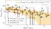 |
Fig. 9 Mass-metallicity plane populated with companions from different samples, adapted from Thorngren et al. (2016), Nasedkin et al. (2024) and Balmer et al. (2024). The orange points show transiting giant exoplanets from Thorngren et al. (2016). The grey points illustrate a set of directly detected planets, and the blue points show a subset that was observed using VLTI/GRAVITY. Both samples were compiled by Nasedkin et al. (2024) and references therein. For context, Jupiter and Saturn are included with the metallicity measurements taken from Guillot (1999). The orange line and confidence interval trace the empirical relation between mass and metallicity for giant exoplanets presented by Thorngren et al. (2016). The black diamond indicates the ratio derived for HIP 99770 b when assuming a solar metallicity for the host. We took the higher metallicity ratios obtained from the host metallic-ity estimates by Paunzen et al. (1999, 2002), and Villaume et al. (2017) into account by presenting the data point with an inflated error bar that reflects a skewed systematic error encompassing the 68% confidence interval of the highest encountered ratio. |
4.4 Comparing evolutionary and atmospheric modelling
To assess whether the bulk parameter values inferred using atmospheric models to fit the spectral energy distribution as discussed in Sect. 4.3 are physically plausible, we compared them to the values implied by self-consistent evolutionary models. To this end, the relations between the companion effective temperature, Teff, and its radius, R, as well as between its effective temperature and surface gravity, log(g), at constant ages (isochrones) and constant masses (evolutionary tracks) as suggested by the AMES-Dusty model are plotted alongside the respective values resulting from sampling the different atmospheric model grids in Fig. 10. We also highlight the Teff-R and Teff-log(g) regions consistent with the AMES-Dusty model at the dynamical mass and age of HIP 99770 b (via its Ks-band magnitude, as explained in Sect. 4.2).
Comparison of these self-consistently inferred parameter regions with the values from the atmospheric modelling implies a poor agreement between the two independent methods. Notably, the DRIFT-PHOENIX results are farthest removed from those of AMES-Dusty in both cases. Fig. 10 reveals that the DRIFT-PHOENIX radius of approximately 0.6 RJup is unrealistic at the ages suggested by both the older and the younger scenario outlined in Sect. 4.2. Similarly, the surface gravity inferred by DRIFT-PHOENIX would necessitate a far more massive body, which we know to be impossible from the orbital analysis in Sect. 3. The effective temperature is reasonably well recovered by the three remaining atmospheric models. However, the radius and surface gravity values from the atmospheric models both show a significant degree of scatter around the feasible parameter regions implied by AMES-Dusty. Seeing that it overlaps with the AMES-Dusty model in both panels, of the three, the Saumon & Marley Cloudy (2008) model performs best, while BT-Settl and Sonora-Diamondback underestimate both radius and surface gravity. Thus, even in cases where the dynamical mass is only loosely constrained around the deuterium-burning threshold, the radius, surface gravity, and effective temperature of the companion as derived from self-consistent evolutionary models still exhibit less scatter than the scatter that is encountered between different atmospheric models.
Going forward, the CHARIS, GRAVITY and NIRC2 observations at hand constitute a suitable data set for testing and gauging atmospheric models in comparison to self-consistent evolutionary models.
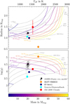 |
Fig. 10 Companion radius, R, and surface gravity, log(g), as a function of effective temperature, Teff. The dotted grey lines indicate isochrones of different ages, the dashed lines illustrate evolutionary tracks, i.e. how a companion of a certain mass evolves over time. The specific masses that the tracks correspond to are indicated by their respective colours. Both the isochrones and the evolutionary tracks are taken from the AMES-Dusty model grid (Chabrier et al. 2000; Allard et al. 2001). The hexagonal bin map in the background shows where a sample of pairs drawn from the mass and K-band magnitude distributions falls when propagated into the parameter planes depicted in the two respective panels using AMES-Dusty. Finally, the values obtained through the atmospheric models applied to the spectral energy distribution of the companion are marked as circles of different colours. |
5 Conclusions
Here, we have presented an updated study of the directly imaged super-Jupiter HIP 99770 b on the basis of two new data sets obtained by the near-infrared interferometric instrument VLTI/GRAVITY. These additional observations added a highly precise astrometric epoch of the companion position relative to its host and extended the temporal coverage available for the system. In addition to confirming the results reported by Currie et al. (2023), the combination of these gains also served to further constrain the orbital solution of the companion. Due to the large relative uncertainty of the host PMa, the resulting companion dynamical mass constraint is still comparatively loose at  . We showed that this situation cannot be remedied by the addition of further relative astrometric epochs. Thus, when its relative uncertainty is large, the dominant nature of the PMa in the orbital sampling procedure prevents further constraints on the dynamical mass of the companion. The only viable method of gaining a firmer grasp on it in the foreseeable future is to exploit the time-series astrometry to be published in Gaia DR4.
While it was unable to strongly constrain the companion mass, the orbital resampling resulted in a significant detection of a non-vanishing eccentricity at  . Although this moderately elevated eccentricity was conceivable even before inclusion of the GRAVITY epoch, the CHARIS and NIRC2 epochs by themselves were also consistent with a low or even vanishing orbital eccentricity, which is now positively ruled out. Instead, HIP 99770 b appears more eccentric than most directly imaged exoplanets.
Comparing the GRAVITY K-band magnitude and dynamical mass of the companion to an evolutionary model, we found them to be consistent with two scenarios. The first implies a planetary mass object at an age of  , the second suggests a more massive object beyond the deuterium-burning threshold at an age of
  . The full spectral energy distribution of the companion is best described by an empirical L8 type object. This agrees with the location of the body on a CMD as compared to a literature population of brown dwarfs and exoplanets.
Next, we fitted the observed spectrum of the companion using different atmospheric models. While each model performed well in terms of its reduced χ2 squared value, the inferred parameter values varied significantly. The use of an informative mass prior based on the dynamical mass of the companion was implemented, but proved ineffective due to its comparative looseness. Employing a firmer dynamical mass constraint as a prior would effect a stronger pull on the posteriors. The inferred enriched metallicity of the companion relative to the solar value is consistent across different models and with the results presented by Zhang et al. (2024).
Finally, the radii, surface gravities, and effective temperatures inferred from the atmospheric models were compared to the results obtained from a self-consistent evolutionary model. This approach revealed the DRIFT-PHOENIX results to be inconsistent with companion’s mass and age for both the younger and older scenario outlined above. While the other models yielded values more in line with the evolutionary approach, this agreement is feeble and we encountered considerable scatter between the models. Despite its current looseness, the dynamical mass of the companion reveals significant incongruities between self-consistent evolutionary and atmospheric models. Not only do the latter infer numerical parameter values that are at odds with the known physics of substellar companions, they are also inconsistent with each other.
The results laid out in this work do not permit us to infer the formation history of HIP 99770 b. That being said, the provided astrometric and spectroscopic data as well as the new constraints they facilitated will support endeavours to do so in the future.
Acknowledgements
This work has made use of data from the European Space Agency (ESA) mission Gaia (https://www.cosmos.esa.int/gaia), processed by the Gaia Data Processing and Analysis Consortium (DPAC, https://www.cosmos.esa.int/web/gaia/dpac/consortium). Funding for the DPAC has been provided by national institutions, in particular the institutions participating in the Gaia Multilateral Agreement. This research has made use of the Jean-Marie Mariotti Center Aspro service5. This research has benefit-ted from the SpeX Prism Spectral Libraries, maintained by Adam Burgasser. S.L. acknowledges the support of the French Agence Nationale de la Recherche (ANR-21-CE31-0017, ExoVLTI) and of the European Union (ERC Advanced Grant 101142746, PLANETES). G.-D.M. acknowledges the support from the European Research Council (ERC) under the Horizon 2020 Framework Program via the ERC Advanced Grant “ORIGINS” (PI: Henning), No. 832428, and via the research and innovation programme “PROTOPLANETS”, grant agreement No. 101002188 (PI: Benisty).
Finally, we would like to thank the anonymous referee whose thorough feedback helped improve the paper.
Appendix A Additional orbital fitting plots
Here, we present additional plots relating to the orbital analysis outlined in Sect. 3. The full corner plot showing how the inclusion of the GRAVITY astrometric epoch affects the posterior sampling of the orbital solution is shown in Fig. A.1.
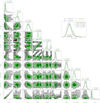 |
Fig. A.1 Corner plot showing the orbital element posteriors of HIP 99770 b. The sampling resulting from only accounting for the previously available data and that obtained upon inclusion of the GRAVITY astrometric epoch (on-axis observation on 31 May 2023) are shown in black and green, respectively. The reported values above the panels showing the marginalised posterior distributions correspond to the median and boundaries of the 68% confidence intervals of the respective element in each sampling run. The top right panel shows companion mass posterior distributions sampled using Gaussian stellar mass priors whose centres were shifted from 1.8 to 1.7 and 1.9M, respectively. |
Appendix B Additional spectral fitting plots
Here, we present additional plots relating to the spectral analysis outlined in Sect. 4.
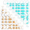 |
Fig. B.1 Lower left: Corner plot showing the posterior sampling of the parameter grid when applying the DRIFT-PHOENIX model to the full set spectroscopic and photometric data presented in Sect 2. Two sampling runs were performed: the results obtained when using no mass prior, that is an uninformative uniform prior, and when using a Gaussian prior based on the dynamical mass obtained from the orbital fit (see Sect. 3) are shown in black and orange, respectively. Above the panels showing the marginalised posterior distributions we report their median values and their differences to the 84th and 16th percentiles in superscript and subscript, respectively. Upper right: Same as lower left for the Sonora Diamondback model grid. |
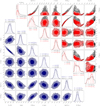 |
Fig. B.2 Same as Fig. B.1 for the BT-Settl and Saumon, Marley Cloudy (2008) model grids in the lower left and upper right panels, respectively. |
Appendix C Correcting for throughput losses
Misplacement between the centre of the GRAVITY science fibre and the target aimed for (in our case the companion) leads to a loss of flux throughput when observing in dual-field mode. To correct for this, we divided the contrast spectra by the normalised coupling efficiency, γ, of the respective observations. These values can be found in Table 1. The coupling efficiency, visualised in Fig. C.1, varies between 1 and 0 and is a function the angular separation between the fibre centre and the target. A comprehensive derivation of its analytic description can be found in Wang et al. (2021).
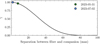 |
Fig. C.1 Normalised coupling efficiency, γ, as a function of the misplacement between the centre of the science fibre and the target. The γ-values used to correct for the throughput losses incurred during the two observations are indicated. |
Appendix D Reduction of GRAVITY on and off-axis spectra
As described in Sect. 2.2, eventually arriving at the combined companion flux spectrum used in the analysis presented in Sect. 4 required converting the contrast spectra into companion flux spectra. This involved multiplying the contrast spectra by calibrator spectra that describe the reference targets (HIP 99770 A and the binary HD 196885 AB for the on and off-axis observations, respectively). In Fig. D.1, we present plots visualising the fitting procedure yielding the best-fit stellar models with Table D.1 listing the parameter values associated to the highest-likelihood sample. We did not account for a potential variability of the star. If present, such variability can impact the goodness of our fits.
These best fitting stellar models,  for HIP 99770 A as well as
  and
and  for the binary components of HD 196885 AB, are the calibrator spectra that were used to convert the observed contrast spectra, C, into companion flux spectra, Fcomp, for both epochs via
 (D.1)
(D.1)
where the operator 〈〉 denotes the averaging over the GRAVITY bandpass. The flux average of the host star  that is required in Eq. (D.1) is obtained from the simultaneous GRAVITY fringe tracker (FT) observations of the host at low spectral resolution. The covariances provided by the GRAVITY pipeline and stellar model uncertainties obtained by taking the standard deviation over 100 randomly drawn samples from the respective posteriors were propagated through each reduction step.
Inferred stellar model atmosphere parameters.
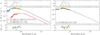 |
Fig. D.1 Inferred stellar model atmospheres for HIP 99770 A (left) and HD 196885 AB (right). The inferred model atmospheres for the A and B components are shown in blue and red, respectively. The combined model is shown in black. The thin lines illustrate 30 randomly drawn samples from the posterior distribution. The photometry and the Gaia XP spectrum included in the fit are shown in orange and green. For greater clarity, only every 10th data point of the Gaia XP spectrum is shown. The top panel shows the filter transmission curve for each photometric point while the bottom panel presents the residuals between the data and the best fit model atmosphere. |
References
- Allard, F., Hauschildt, P. H., Alexander, D. R., Tamanai, A., & Schweitzer, A. 2001, ApJ, 556, 357 [Google Scholar]
- Allard, F., Homeier, D., & Freytag, B. 2012, Philos. Trans. Roy. Soc. Lond. Ser. A, 370, 2765 [NASA ADS] [Google Scholar]
- Balmer, W. O., Pueyo, L., Lacour, S., et al. 2024, AJ, 167, 64 [NASA ADS] [CrossRef] [Google Scholar]
- Balmer, W. O., Franson, K., Chomez, A., et al. 2025, AJ, 169, 30 [NASA ADS] [Google Scholar]
- Baraffe, I., Chabrier, G., Barman, T. S., Allard, F., & Hauschildt, P. H. 2003, A&A, 402, 701 [NASA ADS] [CrossRef] [EDP Sciences] [Google Scholar]
- Bitsch, B., Trifonov, T., & Izidoro, A. 2020, A&A, 643, A66 [EDP Sciences] [Google Scholar]
- Blunt, S., Wang, J. J., Angelo, I., et al. 2020, AJ, 159, 89 [NASA ADS] [CrossRef] [Google Scholar]
- Bodenheimer, P., D’Angelo, G., Lissauer, J. J., Fortney, J. J., & Saumon, D. 2013, ApJ, 770, 120 [NASA ADS] [CrossRef] [Google Scholar]
- Bonnefoy, M., Perraut, K., Lagrange, A. M., et al. 2018, A&A, 618, A63 [NASA ADS] [CrossRef] [EDP Sciences] [Google Scholar]
- Boss, A. P. 1997, Science, 276, 1836 [Google Scholar]
- Bowler, B. P. 2016, PASP, 128, 102001 [Google Scholar]
- Brandt, T. D. 2021, ApJS, 254, 42 [NASA ADS] [CrossRef] [Google Scholar]
- Buchner, J., Georgakakis, A., Nandra, K., et al. 2014, A&A, 564, A125 [NASA ADS] [CrossRef] [EDP Sciences] [Google Scholar]
- Burgasser, A. J., & Splat Development Team 2017, in Astronomical Society of India Conference Series, 14, 7 [Google Scholar]
- Burrows, A., Hubbard, W. B., Lunine, J. I., & Liebert, J. 2001, Rev. Mod. Phys., 73, 719 [Google Scholar]
- Cameron, A. G. W. 1978, Moon Planets, 18, 5 [Google Scholar]
- Cardelli, J. A., Clayton, G. C., & Mathis, J. S. 1989, ApJ, 345, 245 [Google Scholar]
- Carnall, A. C. 2017, arXiv e-prints, [arXiv:1705.05165] [Google Scholar]
- Carson, J., Thalmann, C., Janson, M., et al. 2013, ApJ, 763, L32 [Google Scholar]
- Chabrier, G., Baraffe, I., Allard, F., & Hauschildt, P. 2000, ApJ, 542, 464 [Google Scholar]
- Chauvin, G., Videla, M., Beust, H., et al. 2023, A&A, 675, A114 [NASA ADS] [CrossRef] [EDP Sciences] [Google Scholar]
- Chomez, A., Delorme, P., Lagrange, A. M., et al. 2025, A&A, 697, A99 [NASA ADS] [CrossRef] [EDP Sciences] [Google Scholar]
- Currie, T., Brandt, G. M., Brandt, T. D., et al. 2023, Science, 380, 198 [NASA ADS] [CrossRef] [Google Scholar]
- Cushing, M. C., Marley, M. S., Saumon, D., et al. 2008, ApJ, 678, 1372 [NASA ADS] [CrossRef] [Google Scholar]
- Dupuy, T. J., Liu, M. C., & Ireland, M. J. 2009, ApJ, 692, 729 [NASA ADS] [CrossRef] [Google Scholar]
- Dupuy, T. J., Brandt, G. M., & Brandt, T. D. 2022, MNRAS, 509, 4411 [Google Scholar]
- Feng, F., Anglada-Escudé, G., Tuomi, M., et al. 2019, MNRAS, 490, 5002 [Google Scholar]
- Feroz, F., & Hobson, M. P. 2008, MNRAS, 384, 449 [NASA ADS] [CrossRef] [Google Scholar]
- Feroz, F., Hobson, M. P., & Bridges, M. 2009, MNRAS, 398, 1601 [NASA ADS] [CrossRef] [Google Scholar]
- Foreman-Mackey, D., Hogg, D. W., Lang, D., & Goodman, J. 2013, PASP, 125, 306 [Google Scholar]
- Forgan, D., & Rice, K. 2013, MNRAS, 432, 3168 [Google Scholar]
- Franson, K., Bowler, B. P., Bonavita, M., et al. 2023a, AJ, 165, 39 [NASA ADS] [CrossRef] [Google Scholar]
- Franson, K., Bowler, B. P., Zhou, Y., et al. 2023b, ApJ, 950, L19 [NASA ADS] [CrossRef] [Google Scholar]
- Gaia Collaboration (Prusti, T., et al.) 2016, A&A, 595, A1 [NASA ADS] [CrossRef] [EDP Sciences] [Google Scholar]
- GRAVITY Collaboration (Abuter, R., et al.) 2017, A&A, 602, A94 [NASA ADS] [CrossRef] [EDP Sciences] [Google Scholar]
- GRAVITY Collaboration (Lacour, S., et al.) 2019, A&A, 623, L11 [NASA ADS] [CrossRef] [EDP Sciences] [Google Scholar]
- GRAVITY Collaboration (Nowak, M., et al.) 2020, A&A, 633, A110 [NASA ADS] [CrossRef] [EDP Sciences] [Google Scholar]
- GRAVITY Collaboration (Abuter, R., et al.) 2021, A&A, 647, A59 [NASA ADS] [CrossRef] [EDP Sciences] [Google Scholar]
- Gaia Collaboration (Vallenari, A., et al.) 2023, A&A, 674, A1 [NASA ADS] [CrossRef] [EDP Sciences] [Google Scholar]
- Groff, T., Chilcote, J., Brandt, T., et al. 2017, SPIE Conf. Ser., 10400, 1040016 [Google Scholar]
- Guillot, T. 1999, Planet. Space Sci., 47, 1183 [NASA ADS] [CrossRef] [Google Scholar]
- Helling, C., & Woitke, P. 2006, A&A, 455, 325 [NASA ADS] [CrossRef] [EDP Sciences] [Google Scholar]
- Helling, C., Dehn, M., Woitke, P., & Hauschildt, P. H. 2008, ApJ, 675, L105 [NASA ADS] [CrossRef] [Google Scholar]
- Hinkley, S., Lacour, S., Marleau, G.-D., et al. 2023, A&A, 671, L5 [NASA ADS] [CrossRef] [EDP Sciences] [Google Scholar]
- Jovanovic, N., Martinache, F., Guyon, O., et al. 2015, PASP, 127, 890 [NASA ADS] [CrossRef] [Google Scholar]
- Kervella, P., Arenou, F., Mignard, F., & Thévenin, F. 2019, A&A, 623, A72 [NASA ADS] [CrossRef] [EDP Sciences] [Google Scholar]
- Kervella, P., Arenou, F., & Thévenin, F. 2022, A&A, 657, A7 [NASA ADS] [CrossRef] [EDP Sciences] [Google Scholar]
- Kiefer, F., Hébrard, G., Sahlmann, J., et al. 2019, A&A, 631, A125 [NASA ADS] [CrossRef] [EDP Sciences] [Google Scholar]
- Kratter, K., & Lodato, G. 2016, ARA&A, 54, 271 [NASA ADS] [CrossRef] [Google Scholar]
- Kuzuhara, M., Currie, T., Takarada, T., et al. 2022, ApJ, 934, L18 [NASA ADS] [CrossRef] [Google Scholar]
- Lacour, S., Wang, J. J., Nowak, M., et al. 2020, SPIE Conf. Ser., 11446, 114460O [NASA ADS] [Google Scholar]
- Lambrechts, M., & Johansen, A. 2012, A&A, 544, A32 [NASA ADS] [CrossRef] [EDP Sciences] [Google Scholar]
- Ma, B., & Ge, J. 2014, MNRAS, 439, 2781 [Google Scholar]
- Macintosh, B., Graham, J. R., Barman, T., et al. 2015, Science, 350, 64 [Google Scholar]
- Marleau, G.-D., & Cumming, A. 2014, MNRAS, 437, 1378 [Google Scholar]
- Marleau, G.-D., Coleman, G. A. L., Leleu, A., & Mordasini, C. 2019, A&A, 624, A20 [NASA ADS] [CrossRef] [EDP Sciences] [Google Scholar]
- Marley, M. S., Saumon, D., Visscher, C., et al. 2021, ApJ, 920, 85 [NASA ADS] [CrossRef] [Google Scholar]
- Matthews, E. C., Carter, A. L., Pathak, P., et al. 2024, Nature, 633, 789 [NASA ADS] [CrossRef] [Google Scholar]
- Miles, B. E., Biller, B. A., Patapis, P., et al. 2023, ApJ, 946, L6 [NASA ADS] [CrossRef] [Google Scholar]
- Mollière, P., & Mordasini, C. 2012, A&A, 547, A105 [NASA ADS] [CrossRef] [EDP Sciences] [Google Scholar]
- Mollière, P., Molyarova, T., Bitsch, B., et al. 2022, ApJ, 934, 74 [CrossRef] [Google Scholar]
- Morley, C. V., Mukherjee, S., Marley, M. S., et al. 2024, ApJ, 975, 59 [NASA ADS] [CrossRef] [Google Scholar]
- Mousis, O., Marboeuf, U., Lunine, J. I., et al. 2009, ApJ, 696, 1348 [NASA ADS] [CrossRef] [Google Scholar]
- Murphy, S. J., & Paunzen, E. 2017, MNRAS, 466, 546 [NASA ADS] [CrossRef] [Google Scholar]
- Murphy, S. J., Gray, R. O., Corbally, C. J., et al. 2020, MNRAS, 499, 2701 [NASA ADS] [CrossRef] [Google Scholar]
- Nasedkin, E., Mollière, P., Lacour, S., et al. 2024, A&A, 687, A298 [NASA ADS] [CrossRef] [EDP Sciences] [Google Scholar]
- Nielsen, E. L., De Rosa, R. J., Macintosh, B., et al. 2019, AJ, 158, 13 [Google Scholar]
- Nowak, M., Lacour, S., Abuter, R., et al. 2024, A&A, 687, A248 [NASA ADS] [CrossRef] [EDP Sciences] [Google Scholar]
- Paunzen, E., Andrievsky, S. M., Chernyshova, I. V., et al. 1999, A&A, 351, 981 [Google Scholar]
- Paunzen, E., Handler, G., Weiss, W. W., et al. 2002, A&A, 392, 515 [NASA ADS] [CrossRef] [EDP Sciences] [Google Scholar]
- Pecaut, M. J., & Mamajek, E. E. 2013, ApJS, 208, 9 [Google Scholar]
- Phillips, M. W., Tremblin, P., Baraffe, I., et al. 2020, A&A, 637, A38 [NASA ADS] [CrossRef] [EDP Sciences] [Google Scholar]
- Reggiani, M., Meyer, M. R., Chauvin, G., et al. 2016, A&A, 586, A147 [NASA ADS] [CrossRef] [EDP Sciences] [Google Scholar]
- Sahlmann, J., Ségransan, D., Queloz, D., et al. 2011, A&A, 525, A95 [NASA ADS] [CrossRef] [EDP Sciences] [Google Scholar]
- Saumon, D., & Marley, M. S. 2008, ApJ, 689, 1327 [Google Scholar]
- Schuyer, M. 1985, ESA Bulletin, ISSN 0376-4265 [Google Scholar]
- Spiegel, D. S., Burrows, A., & Milsom, J. A. 2011, ApJ, 727, 57 [Google Scholar]
- Stevenson, A. T., Haswell, C. A., Barnes, J. R., & Barstow, J. K. 2023, MNRAS, 526, 5155 [NASA ADS] [CrossRef] [Google Scholar]
- Stolker, T., Quanz, S. P., Todorov, K. O., et al. 2020, A&A, 635, A182 [EDP Sciences] [Google Scholar]
- Thorngren, D. P., Fortney, J. J., Murray-Clay, R. A., & Lopez, E. D. 2016, ApJ, 831, 64 [NASA ADS] [CrossRef] [Google Scholar]
- Vigan, A., Fontanive, C., Meyer, M., et al. 2021, A&A, 651, A72 [EDP Sciences] [Google Scholar]
- Villaume, A., Conroy, C., Johnson, B., et al. 2017, ApJS, 230, 23 [NASA ADS] [CrossRef] [Google Scholar]
- Vousden, W. D., Farr, W. M., & Mandel, I. 2016, MNRAS, 455, 1919 [NASA ADS] [CrossRef] [Google Scholar]
- Wang, J. J., Vigan, A., Lacour, S., et al. 2021, AJ, 161, 148 [Google Scholar]
- Winterhalder, T. O., Lacour, S., Mérand, A., et al. 2024, A&A, 688, A44 [NASA ADS] [CrossRef] [EDP Sciences] [Google Scholar]
- Woitke, P., & Helling, C. 2003, A&A, 399, 297 [NASA ADS] [CrossRef] [EDP Sciences] [Google Scholar]
- Zhang, Z., Mollière, P., Hawkins, K., et al. 2023, AJ, 166, 198 [NASA ADS] [CrossRef] [Google Scholar]
- Zhang, Y., Xuan, J. W., Mawet, D., et al. 2024, AJ, 168, 131 [Google Scholar]
While the deuterium-burning threshold, which is traditionally assumed to be located at 13 MJup (e.g. Burrows et al. 2001; Spiegel et al. 2011; Mollière & Mordasini 2012), is the conventional choice of classifier between planets and BDs, others have been proposed. For instance, there is evidence that suggests that the turn-over mass of the companion mass function is located far beyond 13 MJup in the region between 25 and 40 MJup (e.g. Sahlmann et al. 2011; Ma & Ge 2014; Reggiani et al. 2016; Kiefer et al. 2019; Stevenson et al. 2023).
Using the relative epoch of periastron, τ, is a sleight of hand that simplifies setting the prior range boundaries. In combination with a reference epoch (tref = 58 849 MJD) and the orbital period, P, it relates to the actual time of periastron passage, tp, via τ = (tp - tref)/P and is thus a dimensionless quantity.
These values have not been rounded to their respective significant figures to facilitate better comparison.
Not to be confused with a deuterium flash, which is a sudden rise, on a logarithmic scale, in the luminosity of an object that begins to burn deuterium only late (e.g. Bodenheimer et al. 2013; Marleau & Cumming 2014).
Available at http://www.jmmc.fr/aspro
All Tables
GRAVITY observation log of the target HIP 99770 b and of the swap calibrator HD 196885 AB.
All Figures
|
Fig. 1 Detection of HIP 99770 b on 31 May 2023. The circular panel indicates the field of view of the GRAVITY science fibre. The map within visualises the |
| In the text | |
|
Fig. 2 Ingredients and outcome of the spectral data reduction. The top three panels show the GRAVITY on-axis contrast spectrum, the associated stellar calibration flux spectrum, and the resulting companion flux spectrum. The same is visualised for the off-axis observation in the three middle panels. Finally, the bottom panel shows the on- and off-axis companion flux spectra alongside the combination of the two. This K-band spectrum of HIP 99770 b is used in Sect. 4. |
| In the text | |
|
Fig. 3 Orbit of HIP 99770 b relative to its host, i.e., fixed at the origin. The visualised orbits were generated from a random subset of 100 parameter sets drawn from the posterior sampling. While the previously available astrometric epochs obtained by SCExAO/CHARIS and Keck/NIRC2 are shown along with their respective uncertainties in ΔRA and ΔDec, knowledge of the correlation coefficient, ρ, allowed us to visualise the VLTI/GRAVITY epoch as a 1 σ confidence ellipse. |
| In the text | |
|
Fig. 4 Marginalised posterior distributions of a subset of the fitted orbital parameters. The black posteriors were sampled considering the previously available data only, while the green posteriors result from the inclusion of the new GRAVITY epoch from 31 May 2023. The median values and intervals between the 16th and 84th percentiles of the distribution are indicated by the horizontal bars. The inferred values resulting from the two runs, which were rounded to the respective significant figure, are displayed at the top of each panel. While technically not one of the parameters explored by the walkers during the sampling procedure, we also plot the period, P, as computed from the other posteriors via Kepler’s third law. The full posterior samplings can be found in Appendix A. |
| In the text | |
|
Fig. 5 Colour-magnitude diagram showing HIP 99770 b, indicated by the black diamond, in relation to a literature population of low-mass stars, brown dwarfs, and exoplanets (see Appendix C of Bonnefoy et al. 2018 and references therein). All ExoGRAVITY targets (ESO ID 1104.C-0651; Lacour et al. 2020) and the companions so far detected via the Gaia-GRAVITY synergy (Winterhalder et al. 2024) are shown in light blue and ochre, respectively. Additionally, isochrones computed using the AMES-Dusty (Chabrier et al. 2000; Allard et al. 2001), AMES-Cond (Allard et al. 2001; Baraffe et al. 2003), and ATMO (Phillips et al. 2020) evolutionary models are shown for two ages: 1 Gyr (solid lines), and 100 Myr (dotted lines). The filters we used to extract these magnitudes and colours from the spectra are Paranal/SPHERE.IRDIS_B_Ks, IRDIS_D_K12_1, and IRDIS_D_K12_2. |
| In the text | |
|
Fig. 6 Goodness-of-fit statistic, Gk, (Cushing et al. 2008) as a function of spectral type when comparing the CHARIS and GRAVITY spectra together and the GRAVITY spectrum alone to empirical spectra. The minimum Gk value in each spectral type bin is indicated by the coloured circles, the error bars display the full Gk range resulting from all empirical spectra within the respective bin. |
| In the text | |
|
Fig. 7 Isochrones from the AMES-Dusty model grid (Chabrier et al. 2000; Allard et al. 2001) in the mass-magnitude plane. The colours indicate the respective age. The solid black lines show the dynamical mass of the companion and the IRDIS_B_Ks filter magnitude, the dotted lines delineate the 16th and 84th percentiles. For the filter magnitude, we adopted a conservative systematic error (see text). The grey colour map in the background visualises the two-dimensional distribution of randomly drawn masses and magnitudes from their respective distributions. The dash-dotted line encircles 68% of all draws. The shoulder in the isochrones in this particular region of the mass-magnitude plane is caused by the onset of deuterium burning and the mass dependence of its time evolution. The panel in the bottom right corner shows the companion age posterior obtained by bootstrapping the drawn mass and magnitude pairs onto the age manifold as defined by the isochrones. |
| In the text | |
|
Fig. 8 Spectral energy distribution of HIP 99770 b. The black points encircled by a white border and connected by a black line show the CHARIS spectrum taken from Currie et al. (2023). The light grey points depict the combination of the on- and off-axis GRAVITY spectra. For visualisation purposes, a rebinned lower resolution GRAVITY spectrum is shown in dark grey encircled by a white border and connected by a dark grey line. Additionally, the mid-infrared photometry data point in the NIRC2.Lp filter is shown as a black diamond encircled by a white border (Currie et al. 2023). The associated horizontal error bar indicates the FWHM of the filter transmission profile. The spectra resulting from the most likely parameter sets determined by the posterior sampling processes are shown for four different atmospheric forward models. SM Cloudy 2008 denotes the cloudy (fsed = 2) Saumon & Marley (2008) model. |
| In the text | |
|
Fig. 9 Mass-metallicity plane populated with companions from different samples, adapted from Thorngren et al. (2016), Nasedkin et al. (2024) and Balmer et al. (2024). The orange points show transiting giant exoplanets from Thorngren et al. (2016). The grey points illustrate a set of directly detected planets, and the blue points show a subset that was observed using VLTI/GRAVITY. Both samples were compiled by Nasedkin et al. (2024) and references therein. For context, Jupiter and Saturn are included with the metallicity measurements taken from Guillot (1999). The orange line and confidence interval trace the empirical relation between mass and metallicity for giant exoplanets presented by Thorngren et al. (2016). The black diamond indicates the ratio derived for HIP 99770 b when assuming a solar metallicity for the host. We took the higher metallicity ratios obtained from the host metallic-ity estimates by Paunzen et al. (1999, 2002), and Villaume et al. (2017) into account by presenting the data point with an inflated error bar that reflects a skewed systematic error encompassing the 68% confidence interval of the highest encountered ratio. |
| In the text | |
|
Fig. 10 Companion radius, R, and surface gravity, log(g), as a function of effective temperature, Teff. The dotted grey lines indicate isochrones of different ages, the dashed lines illustrate evolutionary tracks, i.e. how a companion of a certain mass evolves over time. The specific masses that the tracks correspond to are indicated by their respective colours. Both the isochrones and the evolutionary tracks are taken from the AMES-Dusty model grid (Chabrier et al. 2000; Allard et al. 2001). The hexagonal bin map in the background shows where a sample of pairs drawn from the mass and K-band magnitude distributions falls when propagated into the parameter planes depicted in the two respective panels using AMES-Dusty. Finally, the values obtained through the atmospheric models applied to the spectral energy distribution of the companion are marked as circles of different colours. |
| In the text | |
|
Fig. A.1 Corner plot showing the orbital element posteriors of HIP 99770 b. The sampling resulting from only accounting for the previously available data and that obtained upon inclusion of the GRAVITY astrometric epoch (on-axis observation on 31 May 2023) are shown in black and green, respectively. The reported values above the panels showing the marginalised posterior distributions correspond to the median and boundaries of the 68% confidence intervals of the respective element in each sampling run. The top right panel shows companion mass posterior distributions sampled using Gaussian stellar mass priors whose centres were shifted from 1.8 to 1.7 and 1.9M, respectively. |
| In the text | |
|
Fig. B.1 Lower left: Corner plot showing the posterior sampling of the parameter grid when applying the DRIFT-PHOENIX model to the full set spectroscopic and photometric data presented in Sect 2. Two sampling runs were performed: the results obtained when using no mass prior, that is an uninformative uniform prior, and when using a Gaussian prior based on the dynamical mass obtained from the orbital fit (see Sect. 3) are shown in black and orange, respectively. Above the panels showing the marginalised posterior distributions we report their median values and their differences to the 84th and 16th percentiles in superscript and subscript, respectively. Upper right: Same as lower left for the Sonora Diamondback model grid. |
| In the text | |
|
Fig. B.2 Same as Fig. B.1 for the BT-Settl and Saumon, Marley Cloudy (2008) model grids in the lower left and upper right panels, respectively. |
| In the text | |
|
Fig. C.1 Normalised coupling efficiency, γ, as a function of the misplacement between the centre of the science fibre and the target. The γ-values used to correct for the throughput losses incurred during the two observations are indicated. |
| In the text | |
|
Fig. D.1 Inferred stellar model atmospheres for HIP 99770 A (left) and HD 196885 AB (right). The inferred model atmospheres for the A and B components are shown in blue and red, respectively. The combined model is shown in black. The thin lines illustrate 30 randomly drawn samples from the posterior distribution. The photometry and the Gaia XP spectrum included in the fit are shown in orange and green. For greater clarity, only every 10th data point of the Gaia XP spectrum is shown. The top panel shows the filter transmission curve for each photometric point while the bottom panel presents the residuals between the data and the best fit model atmosphere. |
| In the text | |
Current usage metrics show cumulative count of Article Views (full-text article views including HTML views, PDF and ePub downloads, according to the available data) and Abstracts Views on Vision4Press platform.
Data correspond to usage on the plateform after 2015. The current usage metrics is available 48-96 hours after online publication and is updated daily on week days.
Initial download of the metrics may take a while.