| Issue |
A&A
Volume 699, July 2025
|
|
|---|---|---|
| Article Number | A180 | |
| Number of page(s) | 12 | |
| Section | Stellar structure and evolution | |
| DOI | https://doi.org/10.1051/0004-6361/202555279 | |
| Published online | 07 July 2025 | |
Power density spectra morphologies of seismically unresolved red-giant asteroseismic binaries
1
Heidelberg Institute for Theoretical Studies (HITS), Schloss-Wolfsbrunnenweg 35, D-69118 Heidelberg, Germany
2
Heidelberg University, Centre for Astronomy, Landessternwarte, Königstuhl 12, D-69117 Heidelberg, Germany
⋆ Corresponding author: This email address is being protected from spambots. You need JavaScript enabled to view it.
Received:
23
April
2025
Accepted:
31
May
2025
Abstract
Context. Asteroseismic binaries are two oscillating stars detected in a single light curve. These systems provide robust constraints on stellar models from the combination of dynamical and asteroseismical stellar parameters. Predictions suggested that approximately 200 asteroseismic binaries may exist among the long-cadence Kepler data, and the majority of them consist of two red-clump (core helium burning) stars. However, detecting these systems is challenging when the binary components exhibit oscillations at similar frequencies that are indistinguishable (i.e., unresolved asteroseismic binaries).
Aims. In this study, we predict the morphologies of power density spectra (PDSs) of seismically unresolved red-giant asteroseismic binaries to provide examples that can be used to identify the systems among observed stars.
Methods. We created 5000 artificial asteroseismic binary (AAB) systems by combining the KASOC light curves of red giants with oscillations at similar frequency ranges. To quantify the complexity of the oscillation patterns, we used the maximum signal-to-noise ratio of the background-normalized PDS and Shannon entropy. Additionally, we identified the radial and quadrupole mode pairs for the individual binary component and determined their impact on the PDS morphologies of AABs.
Results. Our results reveal that the majority of AABs (∼47%) consist of the two red-clump stars. The PDSs of AABs generally exhibit increased Shannon entropy and decreased oscillation power compared to individual components. We focused on the ∼8% of AABs whose stellar components have a similar brightness and classified them into four distinct morphologies: (i) single star-like PDSs, whereby oscillations from one component dominate, (ii) aligned, whereby the dominant oscillations in the stars that form the AAB appear at similar frequencies, (iii) partially aligned, whereby some oscillation modes of component stars are aligned while others are not, and (iv) PDSs containing complex structures with unclear mode patterns caused by the misalignment of the mode frequencies of both components.
Conclusions. We found that most AABs with detectable oscillations from both components show complex oscillation patterns. Therefore, unresolved asteroseismic binaries with a low oscillation power and complex oscillation patterns as characterized by high Shannon entropy offer a potential explanation to understand the observed stars with complex PDSs.
Key words: asteroseismology / stars: oscillations
© The Authors 2025
 Open Access article, published by EDP Sciences, under the terms of the Creative Commons Attribution License (https://creativecommons.org/licenses/by/4.0), which permits unrestricted use, distribution, and reproduction in any medium, provided the original work is properly cited.
This article is published in open access under the Subscribe to Open model. This email address is being protected from spambots. You need JavaScript enabled to view it. to support open access publication.
1. Introduction
In the Universe, binary stars are as abundant as single stars (Abt 1983; Raghavan et al. 2010; Duchêne & Kraus 2013; Moe & Di Stefano 2017). Both binary system components share a common formation history, resulting in the same initial chemical composition and age (Prša 2018). This allows us to constrain input parameters for stellar models and study diverse evolutionary paths as a function of mass, luminosity, and their interaction (Sana et al. 2012; Tauris & van den Heuvel 2023; Marchant & Bodensteiner 2024). Additionally, radial velocities from spectroscopic observations and the light curve analysis of an eclipsing system enables us to directly measure the masses and radii of the binary components through dynamical modeling (Andersen 1991; Torres et al. 2010).
Asteroseismology has emerged as a potent method of inferring stellar parameters through scaling relations (Brown et al. 1991; Kjeldsen & Bedding 1995; Huber et al. 2010; Mosser et al. 2013; Hekker 2020), especially for stars with a convective surface layer. These stars show solar-like oscillations, which are intrinsically damped and stochastically excited by the turbulence in the outer layers of the stars. Accordingly, observing these oscillations allowed us to explore the internal structure of the stars. Using the high-precision long-term time series data from the Kepler space mission (Borucki et al. 2010), solar-like oscillations have been detected in about 20 000 red giants (Bedding et al. 2011; Hekker et al. 2011; Huber et al. 2011; Pinsonneault et al. 2014, 2018, 2025; Yu et al. 2018).
Among many identified binary systems with oscillating components (see reviews by Murphy 2018, 2025), solar-like oscillators in these binary systems are particularly valuable. This is because the dynamical masses derived from orbital analysis can provide constraints on the asteroseismic scaling relation and further improve stellar modeling (e.g., Hekker et al. 2010; Gaulme et al. 2013; Beck et al. 2014, 2018, 2022, 2024; Li et al. 2018a; Themessl et al. 2018, and references therein). If both components exhibit oscillations, they provide constraints for both stars and the full potential of asteroseismology. In particular, when oscillations from two stars are detected in a single light curve, we refer to them as asteroseismic binaries, regardless of whether the two components are gravitationally bounded or not. However, only a few asteroseismic binaries have been discovered in which both stars exhibit solar-like oscillations. Appourchaux et al. (2015) reported HD 177412 (KIC 7510397) with solar-like oscillations in two main-sequence binary stars and compared the astrometrical measurement of stellar parameters to the seismic analysis. Moreover, Marcadon et al. (2018) studied the triple star system HD 188753 (KIC 6469154), in which they detected solar-like oscillations in the two brightest components, which have oscillation modes around 2200 and 3300 μHz in the power density spectra (PDSs), respectively. KIC 9163796 has been studied by Beck et al. (2018), and recently by Grossmann et al. (2025), where the power excess of the secondary component is above the Nyquist frequency. For red giants, Themessl et al. (2018) investigated KIC 2568888, which shows the asteroseismic signals of two red-giant components. Further investigations of red-giant asteroseismic binaries in wide binary systems will be presented by Espinoza-Rojas et al. (in prep.).
While asteroseismic binaries with stars that have oscillations in similar frequency ranges are challenging to discover, a select number of systems have been reported. White et al. (2017) presented the main-sequence binary system HD 176465 (KIC 10124866) and derived stellar parameters by analyzing seismic signals of both components, together with an orbital analysis. Li et al. (2018b) analyzed KIC 7107778, which is a non-eclipsing and unresolved asteroseismic subgiant binary system with oscillations of both components that completely overlap. Even though one of two solar-like oscillations is marginally detectable, KIC 9246715 was identified as an eclipsing red-giant binary containing two nearly identical red giants, where the two components exhibit oscillations at similar frequency ranges (see Rawls et al. 2016). With only these few examples, the characteristics of red-giant asteroseismic binaries with overlapping oscillation patterns remain unexplored.
Miglio et al. (2014) conducted population studies on non-eclipsing asteroseismic binaries, predicting that 200 or more such systems should be detectable in Kepler long-cadence data. Their study concluded that combinations of red giants are most prevalent among asteroseismic binaries that have solar-like oscillations of two stars in the frequency spectrum of a single light curve. Most of these binaries are expected to consist of two core-He-burning (CHeB) red giants. Moreover, a recent study by Mazzi et al. (2025) confirmed that binaries consisting of two CHeB red giants represent the largest fraction of systems detected as asteroseismic binaries in their simulation. Red clump (RC) stars that have gone through a helium flash typically have similar core masses and luminosities. Thus, all RC stars exhibit oscillations in a similar frequency range with their frequency of maximum oscillation power (νmax) typically around 20−50 μHz. If two stars with similar νmax are closer to each other in the plane of the sky than the spatial resolution of the telescope, their oscillation signals overlap in the PDS. In this case, their oscillation patterns may look different from single stars. Furthermore, the additional light from the presence of the other star can cause photometric dilution, which reduces the relative flux variations, making the analysis of these systems more difficult.
In this work, we created 5000 seismically unresolved artificial asteroseismic binary (AAB) systems to investigate how they appear in the PDS. Each AAB is composed of two red giants that exhibit oscillations at similar frequency ranges. The resulting variety of PDS morphologies can be considered as a template for identifying potential asteroseismic binary candidates in the observed data. Moreover, we used the Shannon entropy as an estimator to quantify the complexity in the shape of PDS.
Claude Shannon first introduced entropy in communication theory (Shannon 1948). In recent decades, Shannon entropy has been widely applied in the fields of information transmission, computer sciences, astronomy, and so on. In astronomy, Cincotta et al. (1995, 1999) used Shannon entropy to search for periodicity in astronomical time series. Moreover in asteroseismology, the studies by Audenaert et al. (2021) and Audenaert & Tkachenko (2022) used multiscale entropy to capture the complexity of time series at different timescales and classify different types of stellar variability. Furthermore, Suárez (2022) applied Shannon entropy to detect frequency patterns in the PDS of δ Scuti stars, determining the large frequency separation when the entropy in the échelle diagram reaches its minimum. Building on these insights, we use Shannon entropy to provide a measure of the complexity of the PDS with a signal-to-noise ratio (S/N) to investigate different PDS morphologies. Additionally, we focus on the radial (l = 0) and quadrupole (l = 2) oscillation modes of binary components, as they offer insights into the structure of the PDS.
The paper is organized as follows. In Sect. 2 we discuss the time series data of single stars that we used to form AABs. In Sect. 3 we describe the analysis of time series data and PDSs. We also introduce the application of Shannon entropy and how we create AABs. In Sect. 4 we present the analysis of 5000 AABs and examine how the oscillation patterns and power of AABs differ from those of the single stars. Then, we classify the morphologies of AABs. Finally, we discuss the results and conclude in Sect. 5.
2. Time series data
We used red-giant stars from the second APOKASC catalog (APOKASC2; Pinsonneault et al. 2018), which contains 6676 evolved stars. The APOKASC project combined Kepler asteroseismic data with APOGEE spectroscopic data to obtain a precise determination of the stellar properties for a large sample of red giants. We used preprocessed long-cadence (LC; 29.45 min sampling) light curves available from the Kepler Asteroseismic Science Operations Center (KASOC) database1. All of the light curves used in this work were corrected using the KASOC pipeline (see Handberg & Lund 2014 for further details).
We selected stars that have been observed for more than 1000 days and have a filling factor of 0.8 or higher, indicating that each star was monitored for more than 80% of the total observation period. Additionally, we used stars with νmax≥15 μHz, corresponding to stars with a surface gravity (log g) larger than approximately 2.0 dex. We set the upper limit of νmax to 200 μHz, so that power excesses are well below the Nyquist frequency (≈283 μHz for long-cadence Kepler data).
Finally, we assumed that the time series contain oscillations from only a single star. Therefore, we selected stars that are not included in the Kepler Eclipsing Binary Catalog KEBC2 (Prša et al. 2011; Slawson et al. 2011; Kirk et al. 2016), not among the oscillating red-giant stars in binary systems analyzed by Beck et al. (2022, 2024), and not on the list of confirmed chance alignment and contact binary stars from Colman et al. (2017). We also checked non-single stars from Gaia Data Release 3 (DR3) (Gaia Collaboration 2023). Then we focused on red-giant stars whose evolutionary stages were determined by Elsworth et al. (2019) based on four different studies. The final dataset consists of 3063 stars, which contains 1713 red-giant branch (RGB) stars, 1180 RC stars, and 170 secondary clump (2CL) stars.
3. Methods
In this section, we describe how we fit the background model to normalize PDSs in Sect. 3.1.1 and estimate νmax in Sect. 3.1.2. Since we focus on seismically unresolved AAB systems, we applied the same background modeling procedure to both single stars and AABs. To compare the oscillation patterns between individual components that affect the PDS morphologies of AABs, we identified oscillation modes and estimated Δν in the PDSs of the individual stars, as is described in Sect. 3.1.3. We introduce the application of Shannon entropy to investigate the complexity of PDS in Sect. 3.2 and the procedure of creating AABs in Sect. 3.3.
3.1. Asteroseismic analysis
3.1.1. The background model
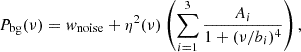
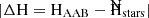
In the Fourier spectrum, power from stellar activity, granulation, and noise (i.e., photon noise and instrumental noise) creates a background on which oscillations are superimposed. Kallinger et al. (2014) found that the instrumental noise is negligible, and thus the noise can be assumed to be white noise. Normalizing these background signals is necessary to study oscillations. We used a prototype of the TACO (Tools for the Automated Characterisation of Oscillations, Hekker et al., in prep.) code to fit a background and obtain νmax. Following the description by Kallinger et al. (2014), the global background fit of the PDS (Pbg(ν)) was modeled as
 (1)
(1)
with wnoise as the white noise, and the sum of three super-Lorentzian profiles representing granulation components occurring at different lengthscales and timescales with their characteristic amplitude, Ai, and characteristic (turnover) frequency, bi (dashed blue lines in Fig. 1). The granulation signals are affected by “apodization”, η(ν), due to the discrete sampling of the flux measurements (see Kallinger et al. 2014 for details).
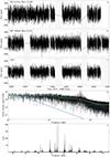 |
Fig. 1. Process of creating the light curve of an AAB star and its PDSs. Panels a and b: Individual light curves of two red-giant stars (KIC 1871314 and KIC 2140446). Panel c: Combined artificial light curve. The shaded light gray regions indicate areas where data points are not available. Panel d: PDS of the light curve from panel c. In this panel, the dashed blue lines represent granulation background components, the dotted gray line indicates the white noise component, and the green line shows the total background fit. Panel e: Background-corrected PDS in the frequency range of νmax±3σenv. The vertical dashed red line in panels d and e indicates the location of νmax estimated as explained in Sect. 3.1.2. |
3.1.2. νmax estimation
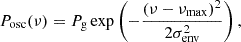
Oscillations are visible as a power excess in the PDS, and we can fit a Gaussian function to estimate νmax, the frequency of maximum oscillation power. The power excess was modeled as
 (2)
(2)
where Pg represents the height of the Gaussian envelope and σenv is the width of the Gaussian envelope. Therefore, the full PDS was modeled as
 (3)
(3)
To estimate parameters in equation (3), we applied a Bayesian Markov chain Monte Carlo framework with affine-invariant ensemble sampling (emcee; Foreman-Mackey et al. 2013). Then we obtained the posterior probability distributions for each parameter, and we adopted the medians of these distributions as an estimate of the expectation values for the parameters and their 16th and 84th percentiles as standard uncertainties. With the global background model, we can create background-corrected PDSs (i.e., the observed PDS Pobs(ν) divided by Pbg(ν)) (see Fig. 1).
3.1.3. Identification of the l = 0, 2 modes, and Δν estimation
We applied the peak-finding method described by García Saravia Ortiz de Montellano et al. (2018) to identify statistically significant Lorentzian-like peaks in the background-normalized PDSs. Each detected peak was fitted using a Lorentzian function given by
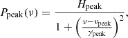
where νpeak, Hpeak, and γpeak represent the central frequency, height, and half-width at half maximum, respectively. We optimized the parameters of each detected peak using maximum likelihood estimation, with the lower limit of the uncertainties calculated by using the Hessian matrix.
To identify the radial (l = 0) and quadrupole (l = 2) modes, we used the “universal pattern” (Mosser et al. 2011) for solar-like oscillations, which predicts the expected mode frequencies. We cross-correlated the observed PDS with the universal pattern within the frequency range νmax±Δν to locate the central l = 0 mode closest to νmax. By using the identified central l = 0 frequencies, we calculated the corresponding l = 2 modes for the given radial order. Subsequently, we identified l = 0,2 modes further away from νmax. Finally, we calculated the large frequency spacing (Δν, the frequency difference between modes of the same spherical degree and consecutive radial orders) from a weighted linear fit to the identified l = 0 modes, considering their frequency uncertainties.
3.2. Shannon entropy
We used the concept of Shannon entropy3 to analyze the PDSs of both individual stars and artificial binaries. The entropy measures both the unpredictability in a probabilistic distribution and the amount of information it provides. Shannon (1948) defined the entropy, H, of a discrete random variable, X, as
 (4)
(4)
where X is a discrete random variable that takes values from the finite set {x1,x2,…,xN}, with corresponding probabilities given by the probability distribution function, p(X=xi). The choice of base for logarithm is typically taken to base 2, which gives the unit of bits.
We estimated p(xi) using a histogram derived from the observed power values in the PDS. For modes with a large linewidth, multiple adjacent peaks are selected as part of a single mode, which could slightly increase the estimated entropy. However, this effect is not significant as the spread in the mode linewidths is not large. Then, we normalized the PDS by the global background fit (Eq. (1)), which provides the power density values equivalent to the S/N. We focused on the frequency range of νmax±3σenv (see the bottom panel of Fig. 1 and the left panels of Fig. 2).
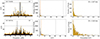 |
Fig. 2. Power density spectra (PDSs) and corresponding histograms of power for two stars with different levels of complexity. The upper panel shows KIC 7949585, which exhibits lower entropy (low complexity), while the lower panel shows KIC 9887555, which has higher entropy (high complexity). The dashed yellow line is the S/N threshold of 4, and the dashed gray line shows the maximum S/N of the selected peaks (see detail about how we select peaks in Sect. 3.2). Peaks that are used in the entropy calculation are marked as yellow circles at the peak maxima position in the left panels, which fall into the yellow bins in the middle panels. In the middle panels, the histograms have a bin width of 1. We normalized their S/Ns to scale the values to the range from 0 to 1 (right panels). The right panels show histograms created by binning the normalized power values into 100 equally spaced bins. These are the probability distributions used in the entropy calculation, Eq. (4). |
A threshold value of S/N was set to reduce the influence of noise peaks in the background-normalized PDS. We empirically chose an S/N threshold of 4 and considered only S/N values of 4 or above. Additionally, to mitigate the effect of occasional spikes with an unusually high S/N, we removed one or two highest peaks if the S/N was above the 99.95th percentile of the S/N distribution.
Then we normalized the selected power values (i.e., only those with S/N ≥ 4) so that they ranged from 0 to 1, with the following transformation:
 (5)
(5)
where S/N indicates the background-normalized power density values in the selected frequency range and max(S/N) represents the highest value among these S/Ns. We created a histogram of the normalized S/N values using 100 bins uniformly distributed over the range [0,1] (see the right panels of Fig. 2). Each bin is labeled as xi (where i in {1, 2, …, 100}). We used this histogram to estimate the probability distribution, p(xi). For each bin labeled as xi, we counted the number of normalized S/N values that fall within that bin and denote this count as ni. The total number of data points across all bins is
 (6)
(6)
We estimated the probability of observing a normalized S/N around xi as
 (7)
(7)
which represents the likelihood of observing a peak at a given normalized power level in the background-normalized PDS. Because the probabilities across all bins must sum to 1, we have:
 (8)
(8)
In cases in which max(S/N) values differ significantly between stars, differences in entropy could partly result from the normalization effect (Eq. (5)) rather than intrinsic differences in oscillation complexity. To mitigate this, we filtered out peaks with extreme S/N values before normalization and used max(S/N) as a complementary parameter. Consequently, entropy robustly highlights exceptionally complex oscillation patterns that would otherwise be difficult to identify (see Fig. 2).
When comparing stars with similar max(S/N) values, entropy provides an even more powerful metric for distinguishing PDSs with different levels of complexity. Specifically, higher entropy reflects a more uniform, less predictable distribution of oscillation powers that conveys a larger amount of information, whereas lower entropy indicates a more predictable distribution with less information content. We calculated the entropy for 3212 observed red-giant stars (3063 from the main dataset and 149 known binary stars, see Fig. 3). Notably, for stars with a similar maximum S/N, the RC star with more prominent peaks exhibits higher entropy values compared to the RGB stars with lower entropy values, and the ones with lower entropy values show a higher likelihood of being suppressed dipole mode stars (see the right panels in Fig. 3). Suppressed dipole mode stars exhibit dipole mode visibility well below expected levels (for more details, see Coppée et al. 2024 and earlier works from e.g. Mosser et al. 2012; Stello et al. 2016; Mosser et al. 2017). Additionally, binary stars exhibit a broad range of entropy values, potentially due to the peaks originating from the orbital modulation in the binary system.
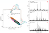 |
Fig. 3. Maximum S/N versus entropy of the background-normalized PDS for 3212 observed red-giant stars, with the y axis plotted on a logarithmic scale. Known binary stars are shown as gray circle (see Sect. 2 for more details of this set of stars). The panels on the right show the background-normalized PDSs corresponding to specific red symbols marked on the left panel. These PDS figures highlight the characteristics associated with their different entropy levels. |
3.3. Construction of AABs
The observed stellar oscillation amplitude is reduced if there is additional light coming from nearby sources within the photometric aperture. As a result, the relative amplitude of the oscillation signal will be smaller compared to the single isolated star, since the detected flux variations are diluted by the total combined light. In the case of a seismically unresolved binary system, the observed light curve reflects the combined photometric fluctuations from both stars within the total flux of the system. Therefore, we incorporated this dilution effect inherently by considering their relative brightness. To calculate the flux contribution of each star, we divided the flux of each star by the combined flux of the two stars. For instance, KIC 1871314 (Kp = 13.38 mag, where Kp is the magnitude in the Kepler band) contributes approximately 19%, while KIC 2140446 (Kp = 11.81 mag) accounts for about 81% (see Fig. 1). Then we multiplied the flux in the light curves of each star with the respective fractional contribution.
Since stars were not observed at exactly the same epochs, we linearly interpolated the time series of the star with fewer observations to match the epochs of the star with more numerous observations. The interpolation was not performed across significant observational gaps. By adding the resulting interpolated flux values from both stars, we created a light curve of AAB. The entire procedure is shown in Fig. 1.
From the 3063 stars in APOKASC2 (see Sect. 2), we can create 4 689 453 unique AABs. To focus on unresolved red-giant asteroseismic binaries that oscillate within a similar frequency range, we selected only those pairs whose difference in νmax is within 10% of their average νmax and a filling factor of 0.8 or higher, resulting in 517 184 artificial binaries. From this subset, we randomly selected 5000 artificial binaries.
4. Results
With 5000 AABs, we explore the various combinations of binary components in terms of their evolutionary stage, νmax, flux ratio, entropy, and the maximum S/N of the background-normalized PDS. We compare the background-normalized PDSs of AABs with the ones of the individual components, investigating differences in entropy and oscillation power. Finally, we classify AABs according to the morphological variations in their background-normalized PDS.
4.1. Distribution of binary components forming AABs
Since we created AABs by using two stars with a similar νmax (see Sect. 3.3), combinations of RC + RC stars dominate (accounting for about 47% of the total, see Fig. 4). The next most common is RGB + RGB (∼27%) due to the largest number of available stars selected in Sect. 2. Following this, pairs of RC + RGB stars make up about 20%, while combinations including 2CL stars are less frequent. We calculated the standard deviation of these fractions via the bootstrap resampling method, by randomly generating 1000 samples of 5000 AABs. We confirmed that the overall distribution remains consistent to the one provided in Fig. 4. While our specific results are restricted to the selected stars in Sect. 2, we expect that unresolved red-giant asteroseismic binaries that are not identified yet are most likely composed of RC + RC stars, consistent with the predictions by Miglio et al. (2014).
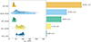 |
Fig. 4. νmax distribution of AABs, with various evolutionary stage combinations of binary components. Below each smoothed curve (normalized to the unit area), a box shows the interquartile range (the 25th to 75th percentiles), with a vertical black line indicating the median. The bar chart on the right shows the percentage of different combinations with their standard deviations. |
Binary components vary in brightness, the maximum S/N of the background-normalized PDS, and entropy. We found that the flux ratios of binary components used to create the set of 5000 AABs are uniformly distributed, with a median around 0.5 (see Fig. 5). We calculated the relative differences in entropy and maximum S/N (Δ=(b−f)/(b+f), where b and f indicate the brighter and fainter stars, respectively). The histograms for relative entropy and maximum S/N differences peak around zero, which indicates that many binary components have similar values in these parameters. This is due to the significant number of pairs that are RC + RC (see Fig. 4), as RC stars have a relatively narrow range of max(S/N) and entropy values (see Fig. 3). In contrast, binary components involving RGB stars show a more gradual relative difference distribution both in max(S/N) and entropy. Moreover, we observe that larger differences in max(S/N) typically correspond to larger differences in entropy. Distributions of these parameters confirm that randomly generated binary components cover a comprehensive range, forming a diverse set of AABs.
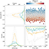 |
Fig. 5. Binary components are characterized by flux ratio, entropy, and the maximum S/N of the background-normalized PDS. The upper right panel shows the distribution of flux ratios against the maximum S/N differences, with points color-coded by entropy differences. The adjacent histograms show the respective distributions. The lower left panel shows the entropy difference distribution. The colors of the histograms have the same meaning as in Fig. 4, with dotted gray lines representing all binary components and the vertical lines indicating the medians. |
4.2. Variations in entropy and S/N between binary components and AABs
Compared to RGB stars, CHeB stars have larger period spacings of dipole mixed modes and higher number of mixed modes with substantial amplitudes which leads to higher complexity in their PDS and higher entropy. Consequently, AABs composed of two CHeB stars typically result in higher entropy than AABs composed of two RGB stars (see Fig. 6). Furthermore, we compare the entropy and maximum S/N of the PDS of AABs with those of their binary components in Fig. 6. Most AABs (∼66%, see Fig. 7) exhibit a lower maximum S/N and higher entropy than their components. The reduced oscillation power in artificial binaries is due to the added flux of the two stars reducing their relative flux amplitudes compared to the individual stars (see Fig. 1). In Fig. 7, the second most common category is characterized by entropy and maximum S/N values that lie between the ones of the individual components (comprising about 15% of AABs). These AABs mostly consist of binary components with significantly different entropies and maximum S/Ns from each other. In particular, many AABs in this category involve RGB stars, as we discussed in Sect. 4.1. On the other hand, only minor differences in entropy and maximum S/N are observed when two CHeB stars form AABs within this category.
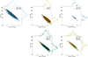 |
Fig. 6. Comparison of maximum S/N (logarithmic scale) and entropy between AABs (star symbols) and their component stars. Histograms along each axis represent the raw counts, with dashed gray lines representing the distributions of all single stars in each panel. |
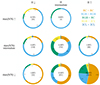 |
Fig. 7. Categorization of the changes in entropy and maximum S/N for AABs compared to their component stars. From left to right, AABs show lower, intermediate, and higher entropy, while from top to bottom, they exhibit higher, intermediate, and lower maximum S/Ns. The widths of the donut charts indicate the total number of AABs in each category, with larger counts indicated as thicker donuts. |
To understand these differences, we calculated the changes in entropy ( ) and maximum S/N (
 ), where
  and
and  indicate the mean value. Small differences are observed when one component star dominates the light contribution to the combined signal or both components have oscillation modes located at similar frequencies, which leads to oscillation patterns of AABs that resemble the dominant frequency patterns (e.g., the first two columns of Fig. 9). In contrast, distinctly different oscillation patterns between binary component stars (e.g., the last two columns in Fig. 9) lead to larger differences in both entropy and the maximum S/N of the resulting AABs, indicating that the magnitude of these differences depends on the oscillation characteristics of the binary components.
4.3. Classification of different PDS morphologies of AABs
The interplay between brightness, intrinsic oscillation power, complexity, and the alignment of oscillation patterns determines the PDS of AABs. In particular, the flux ratio mainly constrains whether oscillations from both stars are visible in the PDS. As the flux ratio increases, oscillation signatures from both stars become more clearly detectable. Therefore, we focused on the 394 AABs with flux ratios ≥0.9 and classified them into the following categories by checking the alignment of their oscillation mode frequencies (see representative examples in Fig. 9, and additional examples in Appendix A).
-
Single star-like AABs, in which oscillations from one component dominate due to the stronger intrinsic oscillation power, i.e., the PDS of AABs resembles that of the dominant star with reduced oscillation power.
-
Aligned AABs, in which the same spherical degrees of oscillation modes of the binary components are located at similar frequencies.
-
Partially aligned AABs, in which some oscillation modes are located at similar frequencies while others are not. In several cases, a radial mode from one star nearly coincides with a quadrupole mode from the other star, creating a distinct peak in the PDS of artificial binaries. As is shown in the third column of Fig. 9, the quadrupole mode frequencies of the star in the upper panel align with the radial mode frequencies of the star in the middle panel. The mixture of dipole and quadrupole modes complicates the identification of the individual oscillation modes in the AABs.
-
Misaligned AABs, in which none of the radial or quadrupole modes have similar frequencies between the binary components. Consequently, the PDS of artificial binaries exhibits a highly complex oscillation pattern. It even becomes challenging to identify the radial modes. These cases also tend to show more significant variations in entropy and maximum S/N compared to those of the individual binary components.
We found that if the frequency differences both in l = 0 and l = 2 are less than about 10% of the mean Δν, it typically indicates aligned cases. AABs with partially aligned binary components show frequency differences typically between 10% and 25%, and differences greater than 25% tend to show totally misaligned components (see Fig. 8). We confirmed these classifications through visual inspection. Importantly, most AABs with a flux ratio ≥0.9 are classified as partially aligned or misaligned (see Table. 1). This implies that red-giant asteroseismic binaries whose components have similar oscillation frequencies are likely to show complex features in their PDSs when oscillations from both components are clearly detectable. Although the entropy values of AABs do not show clear distinctions between the categories, we found that changes in entropy values are larger in partially aligned and misaligned categories, both with a median of |ΔH|≈0.4 bits, compared to aligned cases with a median of |ΔH|≈0.3 bits (see Fig. A.4).
 |
Fig. 8. Scaled frequency differences for the radial (l = 0) versus quadrupole (l = 2) modes of binary components with flux ratios ≥0.9. The relative differences ( |
Results of the PDS morphology classification of AABs with a flux ratio ≥0.9.
5. Discussion and conclusions
In this paper, we have created 5000 artificial asteroseismic binaries to explore the characteristics of unresolved red-giant asteroseismic binaries. This extensive set of AAB systems has allowed us to predict observable features and identify specific spectral signatures useful for recognizing seismically unresolved asteroseismic binaries in the observed data. Among 5000 AABs, about 47% of the AABs consist of two RC stars. Importantly, most of the AABs (about 66%) exhibit increased Shannon entropy and decreased maximum S/N compared to their individual components.
The primary goal of our study has been to investigate the PDS when oscillations from two red giants are present, particularly when they oscillate at similar frequency ranges. Thus, we focused on AABs created from stars with a flux ratio greater than 0.9 (about 8% out of 5000 AABs), where we expected the oscillation signatures from both stars to be detectable.
We classified the PDS morphologies of AABs (flux ratio ≥0.9) into four categories: single star-like, aligned, partially aligned, and misaligned. Most of them were classified in either the partially aligned or misaligned categories. This suggests that seismically unresolved red-giant asteroseismic binaries oscillating at similar frequency ranges are likely to exhibit complex oscillation patterns in their PDS.
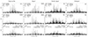 |
Fig. 9. PDS of artificial asteroseismic binaries, which represent various morphological types, along with the corresponding PDS of the individual component stars that created them. Gray peaks indicate filtered out peaks in the entropy calculation (see Sect. 3.2). |
Interestingly, several observed stars exhibit unusually complex oscillation patterns with low oscillation power. In addition to the scenarios such as prolonged mass-loss events extending from the RGB phase into the CHeB phase (e.g., KIC 9508595; Elsworth et al. 2019; Braun 2022) or extreme coupling between pressure- and gravity-mode cavities (e.g. KIC 11299941; Matteuzzi et al. 2023), we propose a scenario in which observed stars with complex PDS may be asteroseismic binaries.
In conclusion, seismically unresolved asteroseismic binaries offer a explanation for the stars observed with complex PDSs. Further observational studies are essential to validate our hypothesis and refine the criteria for identifying unresolved red-giant asteroseismic binaries. Comparing our AABs with actual observations will be crucial for confirming these scenarios and will be presented in a future work.
Acknowledgments
We thank the anonymous referee for their constructive feedback that improved the manuscript considerably. We acknowledge funding from the ERC Consolidator Grant DipolarSound (grant agreement # 101000296). In addition, we acknowledge support from the Klaus Tschira Foundation. This paper includes data collected by the Kepler mission. Funding for the Kepler mission is provided by the NASA Science Mission Directorate.
Throughout this paper, we used “entropy” as shorthand for “Shannon entropy”.
References
- Abt, H. A. 1983, ARA&A, 21, 343 [Google Scholar]
- Andersen, J. 1991, A&A Rev., 3, 91 [Google Scholar]
- Appourchaux, T., Antia, H. M., Ball, W., et al. 2015, A&A, 582, A25 [NASA ADS] [CrossRef] [EDP Sciences] [Google Scholar]
- Audenaert, J., & Tkachenko, A. 2022, A&A, 666, A76 [NASA ADS] [CrossRef] [EDP Sciences] [Google Scholar]
- Audenaert, J., Kuszlewicz, J. S., Handberg, R., et al. 2021, AJ, 162, 209 [NASA ADS] [CrossRef] [Google Scholar]
- Beck, P. G., Hambleton, K., Vos, J., et al. 2014, A&A, 564, A36 [NASA ADS] [CrossRef] [EDP Sciences] [Google Scholar]
- Beck, P. G., Kallinger, T., Pavlovski, K., et al. 2018, A&A, 612, A22 [NASA ADS] [CrossRef] [EDP Sciences] [Google Scholar]
- Beck, P. G., Mathur, S., Hambleton, K., et al. 2022, A&A, 667, A31 [NASA ADS] [CrossRef] [EDP Sciences] [Google Scholar]
- Beck, P. G., Grossmann, D. H., Steinwender, L., et al. 2024, A&A, 682, A7 [NASA ADS] [CrossRef] [EDP Sciences] [Google Scholar]
- Bedding, T. R., Mosser, B., Huber, D., et al. 2011, Nature, 471, 608 [Google Scholar]
- Borucki, W. J., Koch, D., Basri, G., et al. 2010, Science, 327, 977 [Google Scholar]
- Braun, T. A. M. 2022, Master's Thesis, Heidelberg Institute for Theoretical Studies, Germany [Google Scholar]
- Brown, T. M., Gilliland, R. L., Noyes, R. W., & Ramsey, L. W. 1991, ApJ, 368, 599 [Google Scholar]
- Cincotta, P. M., Mendez, M., & Nunez, J. A. 1995, ApJ, 449, 231 [Google Scholar]
- Cincotta, P. M., Helmi, A., Mendez, M., Nunez, J. A., & Vucetich, H. 1999, MNRAS, 302, 582 [Google Scholar]
- Colman, I. L., Huber, D., Bedding, T. R., et al. 2017, MNRAS, 469, 3802 [Google Scholar]
- Coppée, Q., Müller, J., Bazot, M., & Hekker, S. 2024, A&A, 690, A324 [NASA ADS] [CrossRef] [EDP Sciences] [Google Scholar]
- Duchêne, G., & Kraus, A. 2013, ARA&A, 51, 269 [Google Scholar]
- Elsworth, Y., Hekker, S., Johnson, J. A., et al. 2019, MNRAS, 489, 4641 [NASA ADS] [CrossRef] [Google Scholar]
- Foreman-Mackey, D., Hogg, D. W., Lang, D., & Goodman, J. 2013, PASP, 125, 306 [Google Scholar]
- Gaia Collaboration (Arenou, F., et al.) 2023, A&A, 674, A34 [CrossRef] [EDP Sciences] [Google Scholar]
- García Saravia Ortiz de Montellano, A., Hekker, S., & Themeßl, N. 2018, MNRAS, 476, 1470 [CrossRef] [Google Scholar]
- Gaulme, P., McKeever, J., Rawls, M. L., et al. 2013, ApJ, 767, 82 [Google Scholar]
- Grossmann, D. H., Beck, P. G., Mathur, S., et al. 2025, A&A, 696, A42 [NASA ADS] [CrossRef] [EDP Sciences] [Google Scholar]
- Handberg, R., & Lund, M. N. 2014, MNRAS, 445, 2698 [Google Scholar]
- Hekker, S. 2020, Front. Astron. Space Sci., 7, 3 [NASA ADS] [CrossRef] [Google Scholar]
- Hekker, S., Debosscher, J., Huber, D., et al. 2010, ApJ, 713, L187 [Google Scholar]
- Hekker, S., Gilliland, R. L., Elsworth, Y., et al. 2011, MNRAS, 414, 2594 [Google Scholar]
- Huber, D., Bedding, T. R., Stello, D., et al. 2010, ApJ, 723, 1607 [NASA ADS] [CrossRef] [Google Scholar]
- Huber, D., Bedding, T. R., Stello, D., et al. 2011, ApJ, 743, 143 [Google Scholar]
- Kallinger, T., De Ridder, J., Hekker, S., et al. 2014, A&A, 570, A41 [NASA ADS] [CrossRef] [EDP Sciences] [Google Scholar]
- Kirk, B., Conroy, K., Prša, A., et al. 2016, AJ, 151, 68 [Google Scholar]
- Kjeldsen, H., & Bedding, T. R. 1995, A&A, 293, 87 [NASA ADS] [Google Scholar]
- Li, T., Bedding, T. R., Huber, D., et al. 2018a, MNRAS, 475, 981 [Google Scholar]
- Li, Y., Bedding, T. R., Li, T., et al. 2018b, MNRAS, 476, 470 [Google Scholar]
- Marcadon, F., Appourchaux, T., & Marques, J. P. 2018, A&A, 617, A2 [Google Scholar]
- Marchant, P., & Bodensteiner, J. 2024, ARA&A, 62, 21 [NASA ADS] [CrossRef] [Google Scholar]
- Matteuzzi, M., Montalbán, J., Miglio, A., et al. 2023, A&A, 671, A53 [NASA ADS] [CrossRef] [EDP Sciences] [Google Scholar]
- Mazzi, A., Thomsen, J. S., Miglio, A., et al. 2025, A&A, 699, A39 [NASA ADS] [CrossRef] [EDP Sciences] [Google Scholar]
- Miglio, A., Chaplin, W. J., Farmer, R., et al. 2014, ApJ, 784, L3 [CrossRef] [Google Scholar]
- Moe, M., & Di Stefano, R. 2017, ApJS, 230, 15 [Google Scholar]
- Mosser, B., Belkacem, K., Goupil, M. J., et al. 2011, A&A, 525, L9 [CrossRef] [EDP Sciences] [Google Scholar]
- Mosser, B., Elsworth, Y., Hekker, S., et al. 2012, A&A, 537, A30 [NASA ADS] [CrossRef] [EDP Sciences] [Google Scholar]
- Mosser, B., Michel, E., Belkacem, K., et al. 2013, A&A, 550, A126 [CrossRef] [EDP Sciences] [Google Scholar]
- Mosser, B., Belkacem, K., Pinçon, C., et al. 2017, A&A, 598, A62 [NASA ADS] [CrossRef] [EDP Sciences] [Google Scholar]
- Murphy, S. J. 2018, arXiv e-prints [arXiv:1811.12659] [Google Scholar]
- Murphy, S. J. 2025, Contrib. Astron. Obs. Skalnate Pleso, 55, 122 [Google Scholar]
- Pinsonneault, M. H., Elsworth, Y., Epstein, C., et al. 2014, ApJS, 215, 19 [Google Scholar]
- Pinsonneault, M. H., Elsworth, Y. P., Tayar, J., et al. 2018, ApJS, 239, 32 [Google Scholar]
- Pinsonneault, M. H., Zinn, J. C., Tayar, J., et al. 2025, ApJS, 276, 69 [NASA ADS] [CrossRef] [Google Scholar]
- Prša, A. 2018, Modeling and Analysis of Eclipsing Binary Stars; The theory and design principles of PHOEBE (Bristol, UK: IOP Publishing) [Google Scholar]
- Prša, A., Batalha, N., Slawson, R. W., et al. 2011, AJ, 141, 83 [Google Scholar]
- Raghavan, D., McAlister, H. A., Henry, T. J., et al. 2010, ApJS, 190, 1 [Google Scholar]
- Rawls, M. L., Gaulme, P., McKeever, J., et al. 2016, ApJ, 818, 108 [Google Scholar]
- Sana, H., de Mink, S. E., de Koter, A., et al. 2012, Science, 337, 444 [Google Scholar]
- Shannon, C. E. 1948, Bell Syst. Techn. J., 27, 379 [Google Scholar]
- Slawson, R. W., Prša, A., Welsh, W. F., et al. 2011, AJ, 142, 160 [Google Scholar]
- Stello, D., Cantiello, M., Fuller, J., Garcia, R. A., & Huber, D. 2016, PASA, 33 [Google Scholar]
- Suárez, J. C. 2022, Front. Astron. Space Sci., 9, 953231 [Google Scholar]
- Tauris, T. M., & van den Heuvel, E. P. J. 2023, Physics of Binary Star Evolution. From Stars to X-ray Binaries and Gravitational Wave Sources (Princeton University Press) [Google Scholar]
- Themessl, N., Hekker, S., Mints, A., et al. 2018, ApJ, 868, 103 [NASA ADS] [CrossRef] [Google Scholar]
- Torres, G., Andersen, J., & Giménez, A. 2010, A&A Rev., 18, 67 [Google Scholar]
- White, T. R., Benomar, O., Silva Aguirre, V., et al. 2017, A&A, 601, A82 [NASA ADS] [CrossRef] [EDP Sciences] [Google Scholar]
- Yu, J., Huber, D., Bedding, T. R., et al. 2018, ApJS, 236, 42 [NASA ADS] [CrossRef] [Google Scholar]
Appendix A: PDS Morphologies of AABs with different evolutionary stage combinations and their entropy analysis
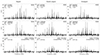 |
Fig. A.1. Same as Figure 9, now for the RGB+RGB where oscillation signatures from both stars are clearly detectable. |
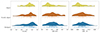 |
Fig. A.4. Distributions of (left) the entropy values (H), (middle) the absolute difference in entropy between AABs and the mean entropy of its component stars ( |
All Tables
All Figures
|
Fig. 1. Process of creating the light curve of an AAB star and its PDSs. Panels a and b: Individual light curves of two red-giant stars (KIC 1871314 and KIC 2140446). Panel c: Combined artificial light curve. The shaded light gray regions indicate areas where data points are not available. Panel d: PDS of the light curve from panel c. In this panel, the dashed blue lines represent granulation background components, the dotted gray line indicates the white noise component, and the green line shows the total background fit. Panel e: Background-corrected PDS in the frequency range of νmax±3σenv. The vertical dashed red line in panels d and e indicates the location of νmax estimated as explained in Sect. 3.1.2. |
| In the text | |
|
Fig. 2. Power density spectra (PDSs) and corresponding histograms of power for two stars with different levels of complexity. The upper panel shows KIC 7949585, which exhibits lower entropy (low complexity), while the lower panel shows KIC 9887555, which has higher entropy (high complexity). The dashed yellow line is the S/N threshold of 4, and the dashed gray line shows the maximum S/N of the selected peaks (see detail about how we select peaks in Sect. 3.2). Peaks that are used in the entropy calculation are marked as yellow circles at the peak maxima position in the left panels, which fall into the yellow bins in the middle panels. In the middle panels, the histograms have a bin width of 1. We normalized their S/Ns to scale the values to the range from 0 to 1 (right panels). The right panels show histograms created by binning the normalized power values into 100 equally spaced bins. These are the probability distributions used in the entropy calculation, Eq. (4). |
| In the text | |
|
Fig. 3. Maximum S/N versus entropy of the background-normalized PDS for 3212 observed red-giant stars, with the y axis plotted on a logarithmic scale. Known binary stars are shown as gray circle (see Sect. 2 for more details of this set of stars). The panels on the right show the background-normalized PDSs corresponding to specific red symbols marked on the left panel. These PDS figures highlight the characteristics associated with their different entropy levels. |
| In the text | |
|
Fig. 4. νmax distribution of AABs, with various evolutionary stage combinations of binary components. Below each smoothed curve (normalized to the unit area), a box shows the interquartile range (the 25th to 75th percentiles), with a vertical black line indicating the median. The bar chart on the right shows the percentage of different combinations with their standard deviations. |
| In the text | |
|
Fig. 5. Binary components are characterized by flux ratio, entropy, and the maximum S/N of the background-normalized PDS. The upper right panel shows the distribution of flux ratios against the maximum S/N differences, with points color-coded by entropy differences. The adjacent histograms show the respective distributions. The lower left panel shows the entropy difference distribution. The colors of the histograms have the same meaning as in Fig. 4, with dotted gray lines representing all binary components and the vertical lines indicating the medians. |
| In the text | |
|
Fig. 6. Comparison of maximum S/N (logarithmic scale) and entropy between AABs (star symbols) and their component stars. Histograms along each axis represent the raw counts, with dashed gray lines representing the distributions of all single stars in each panel. |
| In the text | |
|
Fig. 7. Categorization of the changes in entropy and maximum S/N for AABs compared to their component stars. From left to right, AABs show lower, intermediate, and higher entropy, while from top to bottom, they exhibit higher, intermediate, and lower maximum S/Ns. The widths of the donut charts indicate the total number of AABs in each category, with larger counts indicated as thicker donuts. |
| In the text | |
|
Fig. 8. Scaled frequency differences for the radial (l = 0) versus quadrupole (l = 2) modes of binary components with flux ratios ≥0.9. The relative differences ( |
| In the text | |
|
Fig. 9. PDS of artificial asteroseismic binaries, which represent various morphological types, along with the corresponding PDS of the individual component stars that created them. Gray peaks indicate filtered out peaks in the entropy calculation (see Sect. 3.2). |
| In the text | |
|
Fig. A.1. Same as Figure 9, now for the RGB+RGB where oscillation signatures from both stars are clearly detectable. |
| In the text | |
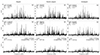 |
Fig. A.2. Same as Figure A.1, now for the RC+RC |
| In the text | |
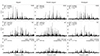 |
Fig. A.3. Same as Figure A.1, now for the RGB+RC |
| In the text | |
|
Fig. A.4. Distributions of (left) the entropy values (H), (middle) the absolute difference in entropy between AABs and the mean entropy of its component stars ( |
| In the text | |
Current usage metrics show cumulative count of Article Views (full-text article views including HTML views, PDF and ePub downloads, according to the available data) and Abstracts Views on Vision4Press platform.
Data correspond to usage on the plateform after 2015. The current usage metrics is available 48-96 hours after online publication and is updated daily on week days.
Initial download of the metrics may take a while.