| Issue |
A&A
Volume 690, October 2024
|
|
|---|---|---|
| Article Number | A324 | |
| Number of page(s) | 11 | |
| Section | Stellar structure and evolution | |
| DOI | https://doi.org/10.1051/0004-6361/202450037 | |
| Published online | 21 October 2024 | |
The radial modes of stars with suppressed dipole modes
1
Heidelberg Institute for Theoretical Studies, Schloss-Wolfsbrunnenweg 35, 69118
Heidelberg, Germany
2
Heidelberg University, Centre for Astronomy, Landessternwarte, Königstuhl 12, 69117
Heidelberg, Germany
Received:
19
March
2024
Accepted:
23
August
2024
Abstract
Context. The Kepler space mission provided high-quality light curves for more than 16 000 red giants. The global stellar oscillations extracted from these light curves carry information about the interior of the stars. Several hundred red giants were found to have low amplitudes in their dipole modes (i.e. they are suppressed dipole-mode stars). A number of hypotheses (involving e.g. a magnetic field, binarity, or resonant mode coupling) have been proposed to explain the suppression of the modes, yet none has been confirmed.
Aims. We aim to gain insight into the mechanism at play in suppressed dipole-mode stars by investigating the mode properties (linewidths, heights, and amplitudes) of the radial oscillation modes of red giants with suppressed dipole modes.
Methods. We selected from the literature suppressed dipole-mode stars and compared the radial-mode properties of these stars to the radial-mode properties of stars in two control samples of stars with typical (i.e. non-suppressed) dipole modes.
Results. We find that the radial-mode properties of the suppressed dipole-mode stars are consistent with the ones in our control samples, and hence not affected by the suppression mechanism.
Conclusions. From this we conclude that (1) the balance between the excitation and damping in radial modes is unaffected by the suppression, and by extrapolation the excitation of the non-radial modes is not affected either; and (2) the damping of the radial modes induced by the suppression mechanism is significantly less than the damping from turbulent convective motion, suggesting that the additional damping originates from the more central non-convective regions of the star, to which the radial modes are least sensitive.
Key words: asteroseismology / stars: interiors / stars: oscillations
Corresponding author; This email address is being protected from spambots. You need JavaScript enabled to view it.
© The Authors 2024
 Open Access article, published by EDP Sciences, under the terms of the Creative Commons Attribution License (https://creativecommons.org/licenses/by/4.0), which permits unrestricted use, distribution, and reproduction in any medium, provided the original work is properly cited.
This article is published in open access under the Subscribe to Open model. This email address is being protected from spambots. You need JavaScript enabled to view it. to support open access publication.
1. Introduction
The space missions CoRoT (Michel et al. 2006) and Kepler (Borucki et al. 2010) transformed asteroseismology into a field of observation-driven research by providing high-quality light curves for more than 100 000 stellar objects, including more than 16 000 red giants (Yu et al. 2018). This transformation is reflected in the major developments of red-giant asteroseismology over the last ten years (see e.g. Chaplin & Miglio 2013; Hekker & Christensen-Dalsgaard 2017; García & Ballot 2019, for reviews). In red giants we observe stochastically excited oscillations undergoing inherently convective damping in the outer regions and diffusive damping in the core (e.g. Houdek et al. 1999; Samadi & Goupil 2001; Dupret et al. 2009). Advancements in the field are mostly due to the detection of non-radial modes in the spectrum of these stars (Hekker et al. 2006; De Ridder et al. 2009). These modes have a mixed character (Beck et al. 2011; Bedding et al. 2011; Mosser et al. 2011a): they behave as gravity modes in the core region (the g-mode cavity) and as pressure modes in the outer layers of the star (the p-mode cavity). These mixed modes therefore carry information from both the p- and g-mode cavities (e.g. Beck et al. 2011; Bedding et al. 2011), while the radial modes that are pure p-modes only carry information from their p-mode cavity, which makes up nearly the entire star (see e.g. Ong & Basu 2019).
Over a decade ago, Mosser et al. (2012) identified a set of red giants with dipole modes with unexpectedly low amplitudes. They showed that, except for the dipole-mode amplitudes, the stars have similar global properties as the other red giants in their sample. An observational analysis of a larger sample of stars with longer light curves was performed by Stello et al. (2016b). They selected red-giant-branch (RGB) stars and computed for each star the dipole-mode visibility (i.e. the ratio of the total power in the dipole modes to the total power in the radial modes). This measurement revealed that the suppression of the dipole modes relative to the radial modes decreases as stars ascend the RGB (i.e. there is less suppression for stars with a weaker coupling between the p- and g-mode cavity; see Stello et al. 2016b). The same methodology applied to quadrupole and octupole modes showed that the suppression is less pronounced for higher spherical degrees (Stello et al. 2016b).
So far, the power in the radial modes of suppressed dipole-mode stars has not been studied. In this work we investigated whether the energy of the radial modes in suppressed dipole-mode stars is different than the energy of the radial modes in stars with dipole modes with typical visibility. We aim to gain insight into the balance between the excitation and damping of these modes as well as into the potential region where the suppression mechanism dominates (i.e. either in the outer regions or in the core) by investigating the total mode power (as per the amplitude and the height) and the mode lifetime (as per the linewidth) of the radial modes.
One mechanism proposed to explain the suppression of the dipole modes is the presence of an internal magnetic field that dominates the regions of the star below a critical depth (Fuller et al. 2015). This depth can be linked to a critical frequency, below which the inward travelling gravity waves are refracted as magnetic waves over a broad range of spherical degrees. This means that the core magnetic field suppresses all contributions from the central regions to the observed non-radial oscillation modes (the ‘magnetic greenhouse effect’). The radial modes remain unaffected. The prediction for the dipole-mode visibilities of red giants made by Fuller et al. (2015) is in agreement with the observed visibilities of Mosser et al. (2012) and Stello et al. (2016b).
Using the individual frequencies of suppressed dipole-mode stars, Mosser et al. (2017) show that some of these stars still have a significant number of mixed dipole modes, albeit with lower amplitudes. This means that the central regions still contribute to the observed non-radial modes. Loi & Papaloizou (2017) propose a mechanism that induces additional damping of the non-radial modes in the presence of a core magnetic field. They show that the contribution of the central regions of the star to the non-radial modes can be partially suppressed through resonances with torsional Alfvén waves. These results suggest that the dipole modes can experience additional damping caused by a core magnetic field and still retain their mixed character. In the case of a strong core magnetic field, Rui & Fuller (2023) show that the contribution of gravity modes should be completely suppressed in red giants. They note that a more general approach (e.g. considering higher-order WKB terms or a non-harmonic time dependence) could potentially allow dipole modes to conserve a mixed character in the presence of a strong core magnetic field.
It is also worth noting that such strong core magnetic fields have been observed in red giants using magnetic frequency splittings (see e.g. Deheuvels et al. 2023). For one of the analysed stars, the reported field is stronger than the critical field derived by Fuller et al. (2015), suggesting that gravity waves should not be able to propagate in the central regions of that particular star. Upon analysis of its power spectrum, Deheuvels et al. (2023) found mixed-mode suppression only at low frequencies. This result is an indication that strong core magnetic fields may be linked to mixed-mode suppression.
Another mechanism that can explain the suppression of dipole modes is the non-linear mode coupling between mixed modes as proposed by Weinberg & Arras (2019). The non-radial-mode visibilities computed with this mechanism (Weinberg et al. 2021) quantitatively match the visibilities of the more evolved red giants reported by Stello et al. (2016b). For this mechanism as well as for the core magnetic field, the radial modes are predicted to be unaffected.
Alternatively, mode suppression could potentially be explained by the presence of a stellar companion as its tidally induced effect can excite non-radial oscillation modes (see e.g. Ivanov et al. 2013), indirectly impacting the properties of the stochastically excited oscillation modes. Statistical results also suggest that the fraction of stars with suppressed dipole modes is larger in binary stars compared to stars that are not known to be part of a binary (see e.g. Themeßl et al. 2017). Due to the non-radial nature of tidal effects, the radial modes are not affected by the tidally induced oscillations (see e.g. Beck et al. 2019, and references therein).
Finally, strong surface magnetic fields inhibit convection in the upper stellar layers, resulting in less stochastic excitation and thus smaller amplitudes for radial and non-radial modes (e.g. Chaplin et al. 2011). Hence, this will have an impact on both the non-radial and radial modes, which is confirmed by Gaulme et al. (2014) and Schonhut-Stasik et al. (2020), who found red giants in eclipsing binaries with no or reduced observable oscillations (i.e. the tidal effect causes enhanced magnetic activity). The presence of a surface magnetic field is the only mechanism that would impact the radial as well as the non-radial modes.
We note here that a high core-rotation rate has also been proposed to explain the suppression of the dipole modes (see e.g. García et al. 2014). García et al. (2014), however, dismissed this mechanism as the cause of the suppression of the dipole modes for KIC 8561221. It is therefore most likely not the main reason for the suppression in the population of suppressed dipole-mode stars, and we do not consider it further here.
In Sect. 2 we specify how we selected RGB stars for our low dipole-mode visibility sample and our control samples, and in Sect. 3 we describe the method we applied to obtain the radial-mode properties of the selected stars. We define the metrics we used to investigate the radial-mode properties in Sect. 4 and present the results of our comparisons thereof in Sect. 5. We dedicate Sect. 6 to the discussion of our results and the conclusions.
2. Sample selection
In this section we describe the selection of stars for our low-visibility sample and how we constructed the control samples. We selected two control samples based on different approaches to compare the distributions of the radial-mode properties of the suppressed dipole-mode stars to those of stars with typical, non-suppressed dipole modes.
For all the stars considered in this work, we used long-cadence kepseismic light curves1. We only selected stars for which we have time series data with a time span longer than 1230 days and a filling factor larger than 0.77. These constraints ensure a high frequency resolution and avoid aliasing effects due to a window effect. We also cross-matched our set of stars with the APOGEE Data Release 17 (DR17) catalogue (Blanton et al. 2017; Abdurro’uf et al. 2022) to obtain stellar effective temperature Teff and metallicity [Fe/H].
We adopted the evolutionary stage (ES) provided by Kallinger (2019) to distinguish between RGB and core-He-burning (CHeB) stars in our sample. If Kallinger (2019) did not provide an ES determination, we determined the ES with the same methodology (Kallinger et al. 2012; Kallinger 2019). This method relies on the frequencies of the three radial modes closest to the frequency of maximal oscillation power, νmax, and can therefore be applied to all stars in our samples consistently, irrespective of their dipole-mode visibility.
2.1. Low-visibility sample
In the literature we find two main sources of stars with suppressed dipole modes, Mosser et al. (2012) and Stello et al. (2016a,2016b). With the available data of Stello et al. (2016a) and Mosser et al. (2017), we selected the candidates for our sample of suppressed dipole-mode stars. As shown by Stello et al. (2016a,b), the distribution in visibility of dipolar modes in their sample of stars is mostly bimodal: one subset of stars centred around 1.5 (typical visibility, Ballot et al. 2011) and another at lower visibility (see Fig. 1). We divided the sample of Stello et al. (2016b) into two regimes using the frequency of maximal oscillation power, νmax, since the bimodality is less pronounced for the most evolved stars (< 70 μHz),
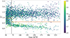 |
Fig. 1. Dipole-visibility distribution as a function of νmax colour-coded by mass (all data from Stello et al. 2016b). The vertical dashed line indicates the boundary between the two νmax regimes, for which the computed visibility thresholds are indicated with horizontal orange lines (see the main text for more details). Note that the negative visibilities are attributed to measurement scatter caused by the uncertainty in the estimation of the background model (see Stello et al. 2016b, for further details). |
-
low, 50 μHz ≤ νmax < 70 μHz,
-
high, νmax ≥ 70 μHz.
In each νmax regime, we fitted a bimodal Gaussian distribution to the dipole-mode visibility distribution and used the intersection of the two Gaussian components as the threshold visibility (see Figs. 1 and 2) and consider the stars with a dipole-mode visibility lower than these thresholds as candidates for our low-visibility sample. In this way, we selected in total 759 stars with low dipole-mode visibility from the sample of Stello et al. (2016a,b). We further included about 40 red giants analysed by Mosser et al. (2017) that are not present in the sample of Stello et al. (2016a,b).
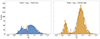 |
Fig. 2. Dipole-mode visibility distribution in the different νmax regimes for the RGB and CHeB stars analysed by Stello et al. (2016b). The thresholds for the visibility are highlighted with a vertical red line. In the low νmax regime, we selected a higher visibility threshold than that obtained from the intersection of the Gaussian components. The dipole-mode visibilities are taken from Stello et al. (2016b). |
After cross-matching with the stars in the APOGEE DR17 our sample consists of 494 red giants, 451 RGB and 43 CHeB stars, with low dipole-mode visibility and spectroscopic parameters from APOGEE DR17. Since the number of RGB stars is an order of magnitude larger than the number of CHeB stars, we focus on the RGB stars for the remainder of this paper.
2.2. Control samples Sp and Sc
For our control samples, we pre-selected RGB stars from the APOKASC2 catalogue (Pinsonneault et al. 2019) with a typical dipole-mode visibility (around 1.5; see e.g. Ballot et al. 2011). From this, we constructed a control sample, Sp, of stars with observed stellar properties similar to those of suppressed dipole-mode stars. To this end, we selected stars by assigning to each star in our low-visibility sample a star with a typical dipole-mode visibility, similar Teff, [Fe/H], and νmax, and large frequency separation, Δν (see Sect. 3 for details on how we obtained the last two parameters). To identify the most suitable configuration for our control sample Sp, we used the Kuhn-Munkres algorithm (Kuhn 1955, 1956; Munkres 1957)2. This algorithm pairs up elements from two distinct sets and finds the configuration of pairs where the sum of the distances d between elements in a pair is the smallest. We defined the distance between two stars in a pair as
![Mathematical equation: $$ \begin{aligned} d^2 =&\frac{{\left( {T_\text{eff,T}-T_\text{eff,} \text{ L}}\right)}^2}{\sigma _{T_\text{eff}}^2} +\frac{{\left(\nu _\text{max,T}-\nu _\text{max,} \text{ L}\right)}^2}{\sigma _{\nu _\text{max}}^2}\nonumber \\&+\frac{{\left( \Delta \nu _\text{T}-\Delta \nu _\text{L}\right)}^2 }{\sigma _{\Delta \nu }^2}+\frac{{\left( {\left[\text{ Fe}/\text{ H}\right]}_\text{T}-{\left[\text{ Fe}/\text{ H}\right]}_\text{L}\right)}^2}{\sigma _{\left[\text{ Fe}/\text{ H}\right]}^2}, \end{aligned} $$](/articles/aa/full_html/2024/10/aa50037-24/aa50037-24-eq1.gif) (1)
(1)
where the subscript T (L) denotes parameters of the star with typical (low) visibility. For the uncertainties, σi, we adopted the following definitions:
 (2)
(2)
![Mathematical equation: $$ \begin{aligned} \sigma _{\left[\text{ Fe}/\text{ H}\right]}&= \sqrt{\sigma _{\left[\text{ Fe}/\text{ H}\right]_\text{T},\text{ intr}}^2+\sigma _{\left[\text{ Fe}/\text{ H}\right]_\text{L},\text{ intr}}^2+2\sigma _{\left[\text{ Fe}/\text{ H}\right], \text{ emp}}^2},\end{aligned} $$](/articles/aa/full_html/2024/10/aa50037-24/aa50037-24-eq3.gif) (3)
(3)
 (4)
(4)
 (5)
(5)
We combined in quadrature the intrinsic uncertainties (subscript intr) of the spectroscopic parameters from APOGEE DR17 and the empirical uncertainties determined to mitigate the discrepancy between asteroseismic and spectroscopic ES classifications (σTeff, emp = 44 K, σ[Fe/H], emp= 0.04 dex; see Elsworth et al. 2019). For the asteroseismic parameters, we combined in quadrature the uncertainties from our code TACO (σνmax, L, and σΔν, L; see Sect. 3 for more information) and the APOKASC2 catalogue (σνmax, T, and σΔν, T; see Pinsonneault et al. 2019).
Having similar spectroscopic and asteroseismic properties does not mean that the masses of the stars in our samples are similar as well. To assure that a different mass distribution does not affect our conclusions, we also generated a second control sample, Sc, by randomly selecting 450 RGB stars with typical dipole-mode visibilities following the cumulative density function (CDF) of the stellar mass distribution observed in the low dipole-mode visibility sample. We estimated the masses M from the asteroseismic scaling relation (see e.g. Ulrich 1986; Brown et al. 1991; Kjeldsen & Bedding 1995) with reference values from Themeßl et al. (2018).
3. Frequency analysis
We performed the frequency analysis of the light curves of the stars in our samples with our peakbagging code TACO (Tools for the Automated Characterisation of Oscillations, Hekker et al., in prep.). In this section we provide an overview of the different steps we took to obtain the radial-mode properties.
First we describe the power density distribution (PDS) with a global model comprising the contribution of the oscillations and of the background (see Kallinger et al. 2014, for more details). We performed the remaining steps in the analysis on the background normalised PDS.
We applied the peak detection method developed by García Saravia Ortiz de Montellano et al. (2018) to detect the peaks in the normalised PDS. We fitted a Lorentzian function,
 (6)
(6)
to each individual detected peak with νpeak, Hpeak, and γpeak the central frequency, height, and half width at half maximum (HWHM) of the peak. We used a maximum likelihood estimation optimisation and computed lower limits of the uncertainties for each peak using a Hessian matrix. Finally, to identify the radial and quadrupole modes, we cross-correlated the observed normalised PDS with a synthetic normalised PDS based on the universal pattern (Mosser et al. 2011b).
We compared the values of νmax and Δν obtained with our code to the results obtained using ABBA (Kallinger 2019) and the FREQ method (Vrard et al. 2018). The comparison shows that our results are in agreement with the results of ABBA and the FREQ method. For νmax the agreement is within one Δν and for Δν within 3σ. Graphical representations of, and additional information about this comparison can be found in Appendix A.
4. Radial-mode properties
The width, height and amplitude of the Lorentzian function (Eq. (6)) describing an oscillation mode carry information about the excitation and damping processes affecting this mode (see e.g. Hekker & Christensen-Dalsgaard 2017, and references therein).
The HWHM γpeak or linewidth Γpeak (full width at half maximum) of a mode are directly related to the mode-damping rate, η, and the mode lifetime, τ,
 (7)
(7)
while Apeak2 (the square of the mode amplitude, i.e. the area under the Lorentzian) and Hpeak (the height of the Lorentzian; see Eq. (6)) are related to the total energy of the mode and are defined as
 (8)
(8)
To condense the information of the different radial modes per star into a single value for the linewidth, amplitude, and height, we defined a global radial linewidth (Γ), amplitude (A), and height (H) as the classical weighted average properties of the three radial modes closest to νmax, namely the modes for which we typically obtain the most precise mode parameters:
 (9)
(9)
 (10)
(10)
 (11)
(11)
with the weights wi = σΓi−2,  , and
, and  defined as a function of the uncertainties σΓi, σAi, and σHi of the ith radial mode. To take the spectral response of the Kepler instrumentation into account, we applied the bolometric correction from Ballot et al. (2011) to the global radial amplitude. In other words, we computed the bolometric amplitude ABol for each star:
 (12)
(12)
We compared our resulting amplitudes and linewidths with values available in the literature. We find that the individual and global radial-mode properties for the stars in our samples are similar to the ones computed in the same way based on the linewidths and amplitudes reported by Kallinger (2019, ABBA). We find agreement with the results based on the data from Kallinger (2019) within 10%, which is within the typical uncertainties. Furthermore, our bolometric amplitudes are consistent with the results obtained by Vrard et al. (2018). However, our global radial-mode linewidths are about 40% smaller than the ones reported by Vrard et al. (2018, i.e. the FREQ method). By comparing the linewidths obtained by Vrard et al. (2018) and Kallinger (2019), we also observe that the linewidths in Vrard et al. (2018) are systematically broader. Although we find that our linewidths are overall narrower for the stars we have in common, the distributions in the global radial-mode parameters are still consistent independent of the datasets that were chosen (the dataset resulting from our code or the datasets from Vrard et al. 2018 or Kallinger 2019). Comparisons of the differences between the datasets can be found in Appendix B.
5. Results
In this section we present the comparison of the CDFs of global radial-mode properties (Γ, H, and ABol) from each control sample to the ones from the low dipole-mode visibility sample (see Figs. 3, 4, and 5). For a quantitative comparison, we used the p-values of the Kolmogorov-Smirnov two-sample test (the KS test hereafter; Hodges 1958), that is, the probability that the two samples are taken from the same underlying distribution (the null hypothesis). A p-value smaller than 1% indicates that we can reject the null hypothesis.
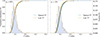 |
Fig. 3. Cumulative distributions of the global linewidth, Γ, for the Sp (left) and Sc (right) control samples (blue) compared to the low-visibility sample (orange). The distributions are shown as histograms in the background (see the right vertical axis for the fraction of stars per bin). The respective p-values of the KS test are shown in the top-left corner of the panels. |
We find that we cannot reject the hypothesis that the distributions in Γ for stars in Sp and Sc are similar to the distribution for suppressed dipole-mode stars (see Fig. 3, where the p-values of the KS test are 82 and 12%, respectively). Since Γ can be related to the average mode-damping rate η, and consequently to the average mode lifetime, τ (see Eq. (7)), we conclude that the convective damping of the radial modes is not altered by the suppression mechanism in suppressed dipole-modes stars.
We additionally find that we cannot reject the hypothesis that the distribution in the bolometric amplitude ABol and H observed in Sp and Sc are similar to the distribution observed for suppressed dipole-mode stars (see Fig. 4, where the p-values of KS test are 27 and 4%, respectively, and Fig. 5, where the p-values are 24 and 53%). This indicates that the total power in the radial modes (scaling as ABol2 and as H) is comparable for stars with low and typical dipole-mode visibility.
We checked that the conclusions we draw from the KS test are not influenced by the randomness implemented in our selection procedures. We therefore generated 5000 realisations of Sp and Sc by randomly selecting a value in the uniformly distributed interval [x−σx,x+σx] for parameter x (Teff, [Fe/H], νmax, Δν, M, Γ, H, and ABol) with uncertainty σx. If we cannot reject the null hypothesis of the KS test for a large majority of these realisations compared to the distribution observed in the low-visibility sample for a given parameter, we conclude that this parameter has a similar distribution for both control and low-visibility sample. For all our parameters we can conclude that the low-visibility and control samples are drawn from the same underlying distribution.
Additionally, we repeated the selection procedure to generate four additional control samples Sc to investigate the influence of the random selection of stars for our control sample. It is important to mention that the same star can be selected for different samples. Again, we find no significant difference in the distributions of the radial-mode properties of low- and typical-visibility stars for any of these samples.
Finally, we checked if our results are independent of the chosen metric in Eqs. (9), (10), and (11). We repeated our comparison with the properties of the three central radial modes, and with the arithmetic mean instead of a weighted mean. For all metrics, we obtain the same results: the distributions of the radial-mode properties for our low-visibility stars are consistent with the properties of the stars in our control samples.
6. Discussion and conclusions
In this study we measured and compared the radial-mode properties of stars with suppressed and non-suppressed dipole modes. We find that the linewidths, and by extension the radial-mode damping rates of the radial modes (see Eq. (7)), are similarly distributed for both types of stars.
We also show that the bolometric amplitudes and the heights of the radial modes are distributed similarly for suppressed and non-suppressed dipole-mode stars. Moreover, since the radial-mode height is independent of the mode inertia, our results show that the mode energy (related to the height and the squared bolometric amplitude) is similarly distributed for both types of stars.
As the mode energy represents the balance between damping and excitation processes (see e.g. Hekker & Christensen-Dalsgaard 2017), we infer from our results that the excitation of the radial modes is unaffected by the mechanism causing the suppressed-dipole modes. Assuming that modes of different spherical degrees are excited in a similar manner, this means that all modes are excited similarly in stars with suppressed and non-suppressed dipole modes. This then leads us to conclude that the observed suppression is caused by additional damping and not by lack of excitation.
The additional source of damping does not significantly affect the radial modes (i.e. the convective damping in radial modes seems unaffected). Under the assumption that the convective damping of the dipole modes is similar to the convective damping of the radial modes (see e.g. Mosser et al. 2017), the additional damping is likely taking place in the stellar core, to which mixed modes are more sensitive than the radial modes.
Since we find that the excitation of the radial modes remains unaffected by the suppression mechanism, our results suggest that a mechanism impacting the mode excitation, such as the presence of a strong surface magnetic field, is likely not the cause of the suppression of the dipole modes in low-visibility stars. For the core magnetic field mechanism, Fuller et al. (2015) note that the magnitude of the core magnetic field is assumed to be too low to affect the radial modes. Different theoretical approaches, such as those developed by Lecoanet et al. (2017) or Loi & Papaloizou (2017), confirm that the presence of a core magnetic field can reduce the dipole-mode amplitudes without affecting the radial modes. Additionally, Cantiello et al. (2016) extended the theoretical analysis of Fuller et al. (2015) by investigating the generation, evolution, and detectability of core magnetic fields and corroborated the results from Fuller et al. (2015). Based on a more general analysis, Rui & Fuller (2023) conclude that above a given magnetic field strength, inward travelling gravity waves will indeed be refracted at a critical depth and will be converted to outgoing slow magnetic waves that dissipate before reaching the stellar surface, leaving the radial-mode properties unaffected.
The resonant mode coupling is a three-wave interaction between mixed modes where a non-radial mode destabilises two other modes with an initially low amplitude (Weinberg & Arras 2019). According to Weinberg et al. (2021), the relatively small displacements near the stellar centre and the large damping rate dominated by convective damping prevent the radial modes from being impacted by this interaction. For red giants in binaries, Beck et al. (2019) conclude that the tidal effects do not significantly impact the radial modes, as no change in the large frequency separation and no radial-mode amplitude modulation were observed. Based on the binary fraction (about 10%) in our low dipole-mode visibility sample, it appears nevertheless unlikely that binarity alone can cause the suppression.
In summary, our findings support either a strong core magnetic field or resonant mode coupling as the suppression mechanism, while surface magnetic fields seem rather unlikely. According to the binary fraction in the suppressed dipole-mode sample, tidal effects are likely not the cause of the mode suppression. Further investigations into core magnetic fields will be presented in a forthcoming work by Müller et al. (in prep.).
Python package munkres, https://github.com/bmc/munkres, © Brian M. Clapper.
Acknowledgments
We thank the referee for their useful comments and remarks that considerably improved the manuscript. We acknowledge funding from the ERC Consolidator Grant DipolarSound (grant agreement # 101000296).
References
- Abdurro’uf, Accetta, K., Aerts, C., et al. 2022, ApJS, 259, 35 [NASA ADS] [CrossRef] [Google Scholar]
- Ballot, J., Barban, C., & Van’t Veer-Menneret, C., 2011, A&A, 531, A124 [NASA ADS] [CrossRef] [EDP Sciences] [Google Scholar]
- Beck, P. G., Bedding, T. R., Mosser, B., et al. 2011, Science, 332, 205 [Google Scholar]
- Beck, P. G., Mathis, S., Kallinger, T., García, R. A., & Benbakoura, M. 2019, EAS Pub. Ser., 82, 119 [NASA ADS] [CrossRef] [EDP Sciences] [Google Scholar]
- Bedding, T. R., Mosser, B., Huber, D., et al. 2011, Nature, 471, 608 [Google Scholar]
- Blanton, M. R., Bershady, M. A., Abolfathi, B., et al. 2017, AJ, 154, 28 [Google Scholar]
- Borucki, W. J., Koch, D., Basri, G., et al. 2010, Science, 327, 977 [Google Scholar]
- Brown, T. M., Gilliland, R. L., Noyes, R. W., & Ramsey, L. W. 1991, ApJ, 368, 599 [Google Scholar]
- Cantiello, M., Fuller, J., & Bildsten, L. 2016, ApJ, 824, 14 [NASA ADS] [CrossRef] [Google Scholar]
- Chaplin, W. J., & Miglio, A. 2013, ARA&A, 51, 353 [Google Scholar]
- Chaplin, W. J., Bedding, T. R., Bonanno, A., et al. 2011, ApJ, 732, L5 [Google Scholar]
- De Ridder, J., Barban, C., Baudin, F., et al. 2009, Nature, 459, 398 [Google Scholar]
- Deheuvels, S., Li, G., Ballot, J., & Lignières, F. 2023, A&A, 670, L16 [NASA ADS] [CrossRef] [EDP Sciences] [Google Scholar]
- Dupret, M. A., Belkacem, K., Samadi, R., et al. 2009, A&A, 506, 57 [NASA ADS] [CrossRef] [EDP Sciences] [Google Scholar]
- Elsworth, Y., Hekker, S., Johnson, J. A., et al. 2019, MNRAS, 489, 489 [Google Scholar]
- Fuller, J., Cantiello, M., Stello, D., Garcia, R. A., & Bildsten, L. 2015, Science, 350, 423 [Google Scholar]
- García, R. A., & Ballot, J. 2019, Liv. Rev. Sol. Phys., 16, 4 [Google Scholar]
- García, R. A., Pérez Hernández, F., Benomar, O., et al. 2014, A&A, 563, A84 [NASA ADS] [CrossRef] [EDP Sciences] [Google Scholar]
- García Saravia Ortiz de Montellano, A., Hekker, S., & Themeßl, N. 2018, MNRAS, 476, 1470 [CrossRef] [Google Scholar]
- Gaulme, P., Jackiewicz, J., Appourchaux, T., & Mosser, B. 2014, ApJ, 785, 5 [NASA ADS] [CrossRef] [Google Scholar]
- Hekker, S., & Christensen-Dalsgaard, J. 2017, A&ARv, 25, 1 [Google Scholar]
- Hekker, S., Aerts, C., De Ridder, J., & Carrier, F. 2006, A&A, 458, 931 [NASA ADS] [CrossRef] [EDP Sciences] [Google Scholar]
- Hodges, J. L. 1958, Arkiv for Matematik, 3, 469 [NASA ADS] [CrossRef] [Google Scholar]
- Houdek, G., Balmforth, N. J., Christensen-Dalsgaard, J., & Gough, D. O. 1999, A&A, 351, 582 [NASA ADS] [Google Scholar]
- Ivanov, P. B., Papaloizou, J. C. B., & Chernov, S. V. 2013, MNRAS, 432, 2339 [Google Scholar]
- Kallinger, T. 2019, ArXiv e-prints [arXiv:1906.09428] [Google Scholar]
- Kallinger, T., Hekker, S., Mosser, B., et al. 2012, A&A, 541, A12 [NASA ADS] [CrossRef] [EDP Sciences] [Google Scholar]
- Kallinger, T., De Ridder, J., Hekker, S., et al. 2014, A&A, 570, A41 [NASA ADS] [CrossRef] [EDP Sciences] [Google Scholar]
- Kjeldsen, H., & Bedding, T. R. 1995, A&A, 293, 87 [NASA ADS] [Google Scholar]
- Kuhn, H. W. 1955, Naval Res. Logist. Q., 2, 83 [CrossRef] [Google Scholar]
- Kuhn, H. W. 1956, Naval Res. Logist. Q., 3, 253 [CrossRef] [Google Scholar]
- Lecoanet, D., Vasil, G. M., Fuller, J., Cantiello, M., & Burns, K. J. 2017, MNRAS, 466, 2181 [Google Scholar]
- Loi, S. T., & Papaloizou, J. C. B. 2017, MNRAS, 467, 3212 [NASA ADS] [Google Scholar]
- Michel, E., Baglin, A., Auvergne, M., et al. 2006, ESA Spec. Pub., 306, 39 [Google Scholar]
- Mosser, B., Barban, C., Montalbán, J., et al. 2011a, A&A, 532, A86 [NASA ADS] [CrossRef] [EDP Sciences] [Google Scholar]
- Mosser, B., Belkacem, K., Goupil, M. J., et al. 2011b, A&A, 525, L9 [CrossRef] [EDP Sciences] [Google Scholar]
- Mosser, B., Elsworth, Y., Hekker, S., et al. 2012, A&A, 537, A30 [NASA ADS] [CrossRef] [EDP Sciences] [Google Scholar]
- Mosser, B., Belkacem, K., Pinçon, C., et al. 2017, A&A, 598, A62 [NASA ADS] [CrossRef] [EDP Sciences] [Google Scholar]
- Munkres, J. 1957, J. Soc. Indust. Appl. Math., 5, 32 [CrossRef] [Google Scholar]
- Ong, J. M. J., & Basu, S. 2019, ApJ, 870, 41 [CrossRef] [Google Scholar]
- Pinsonneault, M. H., Elsworth, Y. P., Tayar, J., et al. 2019, VizieR Online Data Catalog:J/ApJS/239/32 [Google Scholar]
- Rui, N. Z., & Fuller, J. 2023, MNRAS, 523, 582 [NASA ADS] [CrossRef] [Google Scholar]
- Samadi, R., & Goupil, M. J. 2001, A&A, 370, 136 [NASA ADS] [CrossRef] [EDP Sciences] [Google Scholar]
- Schonhut-Stasik, J., Huber, D., Baranec, C., et al. 2020, ApJ, 888, 34 [NASA ADS] [CrossRef] [Google Scholar]
- Stello, D., Cantiello, M., Fuller, J., et al. 2016a, Nature, 529, 364 [Google Scholar]
- Stello, D., Cantiello, M., Fuller, J., Garcia, R. A., & Huber, D. 2016b, PASA, 33 [CrossRef] [Google Scholar]
- Themeßl, N., Hekker, S., & Elsworth, Y. 2017, Eur. Phys. J. Web Conf., 160, 05009 [CrossRef] [EDP Sciences] [Google Scholar]
- Themeßl, N., Hekker, S., Southworth, J., et al. 2018, MNRAS, 478, 4669 [Google Scholar]
- Ulrich, R. K. 1986, ApJ, 306, L37 [Google Scholar]
- Vrard, M., Kallinger, T., Mosser, B., et al. 2018, A&A, 616, A94 [NASA ADS] [CrossRef] [EDP Sciences] [Google Scholar]
- Weinberg, N. N., & Arras, P. 2019, ApJ, 873, 67 [NASA ADS] [CrossRef] [Google Scholar]
- Weinberg, N. N., Arras, P., & Pramanik, D. 2021, ApJ, 918, 70 [NASA ADS] [CrossRef] [Google Scholar]
- Yu, J., Huber, D., Bedding, T. R., et al. 2018, ApJS, 236, 42 [NASA ADS] [CrossRef] [Google Scholar]
Appendix A: Comparison of νmax and Δν with literature values
In this section we compare the values of νmax and Δν obtained with our code to the values found in the literature. We find agreement between our results and the data from Vrard et al. (2018) and Kallinger (2019) for the stars we have in common with their samples (about 70% of our samples). We show in Fig. A.1 and A.2 as well as in Fig. A.3 and A.4 the difference in νmax and Δν between our results for our low-visibility sample, Sc and Sp and the data published by respectively Kallinger (2019) and Vrard et al. (2018) as a function of their uncertainties. We defined the uncertainty on the difference in νmax as one Δν and on the difference in Δν as the combination of the individual uncertainties in quadrature (similar to e.g. in Eq. 5). We find that our values for νmax are within 1 Δν and Δν within 3σ of the given uncertainties. The few outliers in the differences of Δν are caused by a different number of detected radial modes.
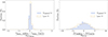 |
Fig. A.1. Difference between the νmax (left) and Δν (right) derived in this work and the results of ABBA (Kallinger 2019) expressed in σ for stars in the low-visibility sample (orange) and Sc (blue). |
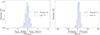 |
Fig. A.3. Same as in Fig. A.1, but now for a comparison with the FREQ results (Vrard et al. 2018). |
Appendix B: Comparison of individual linewidths, amplitudes, and heights with literature values
In this section we compare the values of the linewidths, amplitudes and heights obtained with our code to the values found in the literature. Kallinger (2019) and Vrard et al. (2018) do not report values for the heights of the detected peaks. We therefore computed the heights using Eq. 8 with the reported values for the linewidths and amplitudes. We find that our results are in agreement with the values from Kallinger (2019, see our Figs. B.1 and B.2). By comparing our results of our low-visibility sample and our control samples with the values of Vrard et al. (2018, see our Figs. B.3 and B.4), we find that our linewidths are about 40% narrower than their linewidths (i.e. there is an offset between the two sets of parameters). A similar offset is as expected also observed in the mode heights. These values for the linewidths and heights are, however, still within 3σ, three times the combined uncertainty in quadrature. By comparing the linewidths obtained by Vrard et al. (2018) and Kallinger (2019), we also observe that the linewidths in Vrard et al. (2018) are systematically broader. Our results are overall in agreement with the values from Vrard et al. (2018) for the stars present in both samples. Our distributions of our radial-mode parameters are therefore consistent with the distributions obtained with the values of Vrard et al. (2018) and Kallinger (2019) for the stars we have in common.
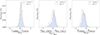 |
Fig. B.1. Difference between the linewidths (left), bolometric amplitudes (middle), and heights (right) based on our results and the Kallinger (2019) data for stars in the low-visibility sample (orange) and Sc (blue). |
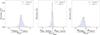 |
Fig. B.3. Same as in Fig. B.1, but now for the comparison with the FREQ results (Vrard et al. 2018). |
All Figures
|
Fig. 1. Dipole-visibility distribution as a function of νmax colour-coded by mass (all data from Stello et al. 2016b). The vertical dashed line indicates the boundary between the two νmax regimes, for which the computed visibility thresholds are indicated with horizontal orange lines (see the main text for more details). Note that the negative visibilities are attributed to measurement scatter caused by the uncertainty in the estimation of the background model (see Stello et al. 2016b, for further details). |
| In the text | |
|
Fig. 2. Dipole-mode visibility distribution in the different νmax regimes for the RGB and CHeB stars analysed by Stello et al. (2016b). The thresholds for the visibility are highlighted with a vertical red line. In the low νmax regime, we selected a higher visibility threshold than that obtained from the intersection of the Gaussian components. The dipole-mode visibilities are taken from Stello et al. (2016b). |
| In the text | |
|
Fig. 3. Cumulative distributions of the global linewidth, Γ, for the Sp (left) and Sc (right) control samples (blue) compared to the low-visibility sample (orange). The distributions are shown as histograms in the background (see the right vertical axis for the fraction of stars per bin). The respective p-values of the KS test are shown in the top-left corner of the panels. |
| In the text | |
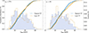 |
Fig. 4. Same as Fig. 3, but now for bolometric amplitude, ABol. |
| In the text | |
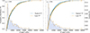 |
Fig. 5. Same as Fig. 3, but now for height, H. |
| In the text | |
|
Fig. A.1. Difference between the νmax (left) and Δν (right) derived in this work and the results of ABBA (Kallinger 2019) expressed in σ for stars in the low-visibility sample (orange) and Sc (blue). |
| In the text | |
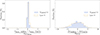 |
Fig. A.2. Same as in Fig. A.1, but now for Sp (blue). |
| In the text | |
|
Fig. A.3. Same as in Fig. A.1, but now for a comparison with the FREQ results (Vrard et al. 2018). |
| In the text | |
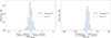 |
Fig. A.4. Same as in Fig. A.3, but now for Sp (blue). |
| In the text | |
|
Fig. B.1. Difference between the linewidths (left), bolometric amplitudes (middle), and heights (right) based on our results and the Kallinger (2019) data for stars in the low-visibility sample (orange) and Sc (blue). |
| In the text | |
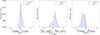 |
Fig. B.2. Same as in Fig. B.1, but now for Sp (blue). |
| In the text | |
|
Fig. B.3. Same as in Fig. B.1, but now for the comparison with the FREQ results (Vrard et al. 2018). |
| In the text | |
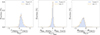 |
Fig. B.4. Same as in B.3, but now for Sp (blue). |
| In the text | |
Current usage metrics show cumulative count of Article Views (full-text article views including HTML views, PDF and ePub downloads, according to the available data) and Abstracts Views on Vision4Press platform.
Data correspond to usage on the plateform after 2015. The current usage metrics is available 48-96 hours after online publication and is updated daily on week days.
Initial download of the metrics may take a while.