| Issue |
A&A
Volume 699, July 2025
|
|
|---|---|---|
| Article Number | A205 | |
| Number of page(s) | 20 | |
| Section | Extragalactic astronomy | |
| DOI | https://doi.org/10.1051/0004-6361/202554707 | |
| Published online | 09 July 2025 | |
The Close AGN Reference Survey (CARS)
Long-term spectral variability study of the changing-look AGN Mrk 1018
1
Leibniz-Institut für Astrophysik Potsdam, An der Sternwarte 16, 14482 Potsdam, Germany
2
Nicolaus Copernicus Astronomical Center of the Polish Academy of Sciences, ul. Bartycka 18, 00-716 Warszawa, Poland
3
Department of Astronomy, The University of Texas at Austin, 2515 Speedway, Stop C1400, Austin, Texas 78712-1205, US
4
MIT Kavli Institute for Astrophysics and Space Research, 77 Massachusetts Ave., Cambridge, MA 02139, USA
5
Observatoire de Paris, LUX, Collège de France, CNRS, PSL University, Sorbonne University, 75014, Paris, France
6
Centre for Astrophysics, University of Southern Queensland, 37 Sinnathamby Boulevard, Springfield, Qld 4300, Australia
7
Instituto de Estudios Astrofísicos, Facultad de Ingeniería y Ciencias, Universidad Diego Portales, Av. Ejército Libertador 441, Santiago, Chile
8
Department of Physics, Informatics and Mathematics, University of Modena and Reggio Emilia, 41125 Modena, Italy
9
Max-Planck-Institut für Astronomie, Königstuhl 17, D-69117 Heidelberg, Germany
10
Department of Astronomy and Astrophysics, University of California San Diego, La Jolla, CA 92093, USA
⋆ Corresponding author.
Received:
23
March
2025
Accepted:
23
May
2025
Abstract
Context. Changing-look active galactic nuclei (CLAGNs) are accreting supermassive black hole systems that undergo variations in optical spectral type driven by major changes in accretion rate. The CLAGN Mrk 1018 has undergone two transitions, a brightening event in the 1980s and a transition back to a faint state over the course of 2–3 years in the early 2010s.
Aims. We characterize the evolving physical properties of the source's inner accretion flow, particularly during the bright-to-faint transition, as well as the morphological properties of its parsec-scale circumnuclear gas.
Methods. We modeled archival X-ray spectra from XMM-Newton, Chandra, Suzaku, and Swift using physically motivated models to characterize X-ray spectral variations and tracked the Fe Kα line flux. We also quantified Mrk 1018's long-term multiwavelength spectral variability from optical/UV to the X-rays.
Results. Over the duration of the bright-to-faint transition, the UV and hard X-ray flux fell by differing factors, roughly 24 and 8, respectively. The soft X-ray excess faded and was not detected by 2021. In the faint state, when the Eddington ratio drops to log(Lbol/LEdd)≲−1.7, the hot X-ray corona photon index shows a “softer-when-fainter” trend that is similar to what is seen in some black hole X-ray binaries and samples of low-luminosity AGNs. Finally, the Fe Kα line flux has dropped by only half the factor of the drop in the X-ray continuum.
Conclusions. The transition from the bright state to the faint state is consistent with the inner accretion flow transitioning from a geometrically thin disk to an ADAF-dominated state, with the warm corona disintegrating or becoming energetically negligible, while the X-ray-emitting hot flow becomes energetically dominant. Meanwhile, narrow Fe Kα emission has not yet fully responded to the drop in its driving continuum, likely because its emitter extends up to roughly 10 pc.
Key words: galaxies: active / X-rays: galaxies / quasars: individual: Markarian 1018
© The Authors 2025
 Open Access article, published by EDP Sciences, under the terms of the Creative Commons Attribution License (https://creativecommons.org/licenses/by/4.0), which permits unrestricted use, distribution, and reproduction in any medium, provided the original work is properly cited.
This article is published in open access under the Subscribe to Open model. This email address is being protected from spambots. You need JavaScript enabled to view it. to support open access publication.
1. Introduction
Active galactic nuclei (AGNs) are powered by accretion onto supermassive black holes (Sołtan 1982) and can emit from the radio band up to gamma rays. Based on its optical spectrum, a Seyfert AGN can be classified into two general types: type 1, where broad emission lines – full width at half maximum (FWHM) ≳ 1000 km s−1 – and narrow forbidden emission lines are present, and type 2, where broad emission lines are absent and only narrow forbidden emission lines can be observed. Intermediate types (1.2, 1.5, 1.8, and 1.9; Osterbrock & Koski 1976) span an intermediate range of broad line properties. For example, type 1.9 sources exhibit a broad Hα emission line but broad Hβ is not detected.
Accretion onto compact objects is generally observed to be a dynamic and hence temporally variable process. Persistently accreting Seyfert AGNs exhibit stochastic variability up to a factor of ∼10–20 in the X-rays (e.g., Markowitz & Edelson 2004) and from a few percent to up to a factor of approximately five in the optical (e.g., Uttley & Mchardy 2004) on timescales ranging from a few days to a few years. A leading mechanism behind stochastic variability is inwardly propagating fluctuations in the local mass accretion rate (Ingram & Done 2011) induced by, for example, fluctuations associated with the magneto-rotational instability (Balbus & Hawley 1991). The community has accumulated over 200 observations of Seyferts and quasars that exhibit extreme continuum variability significantly in excess of the “normal” stochastic variability accompanied by changes to their optical spectral type. Specifically, the optical spectral type changes as one or more broad emission lines appear or disappear. Recent select examples include 1ES 1927+654 (Ricci et al. 2020), Mrk 590 (Denney et al. 2014), and NGC 2617 (Shappee et al. 2014). In most cases, optical spectral changes are driven by changes in the underlying ionizing continuum luminosity rather than in line-of-sight obscuration (Korista et al. 1995, 1997; Korista & Goad 2000; Wu et al. 2023). Results generally support that the prime mechanism driving these continuum luminosity variations is large changes in accretion rate (e.g., LaMassa et al. 2015; Zeltyn et al. 2024; Ricci & Trakhtenbrot 2023) due to major changes in the structure of the accretion flow (e.g., Noda & Done 2018), instabilities originating in the disk (e.g., Lightman & Eardley 1974), or tidal disruption events (TDEs) occurring in AGNs (Trakhtenbrot et al. 2019; Homan et al. 2023)1.
For changing-look AGNs (CLAGNs), whose transient variability is driven by drastic changes in accretion rate, a broad range of behavior has been observed in the X-ray and broadband continuum spectrum. Some sources exhibit drastic changes in X-ray spectral shape with rapid spectral hardening or softening alongside a decrease or increase in multi-band flux. For example, Ricci et al. (2020) reported extreme X-ray spectral softening in the CLAGN 1ES 1927+654 due to the drastic weakening of X-rays above ∼2.0 keV, which is attributed to the destruction of the hard X-ray emitting hot corona. However, after the CLAGN transition in 2017, the hard X-ray-emitting hot corona of CLAGN 1ES 1927+654 recovered (Ricci et al. 2020). Subsequent multiwavelength monitoring has indicated that the accretion flow transitioned from a slim disk to a thin disk two years after the outburst (Li et al. 2024). Ghosh et al. (2022) reported rapid variability in the hot-corona X-ray photon index Γ during the long-term flaring in the CLAGN source Mrk 590. In contrast, some other CLAGNs have exhibited large changes in flux with no significant detectable changes in spectral shape (e.g., LaMassa et al. 2015; Kollatschny et al. 2023; Saha et al. 2023). Furthermore, over a dozen sources (so far) are also known to exhibit repeat CLAGN events (Wang et al. 2025). All of these sources demonstrate that CLAGN transitions induce a broad range of divergent changes in the behavior of the multiwavelength spectra. Notably, characterizing the spectral behavior of each individual source can help reveal the unique characteristics of their inner accretion flow.
Markarian 1018 (Mrk 1018) is a galaxy merger remnant system that hosts an AGN at its center. The AGN was initially classified to be of type 1.9 (Osterbrock 1981), and subsequently its type has changed twice: from type 1.9 to type 1 by 1984 (Cohen et al. 1986) and from type 1 to type 1.9, detected in 2016 (McElroy et al. 2016). The later transition was accompanied by a drop in optical flux. Over the past two decades, X-ray, optical, and UV monitoring of the source have revealed that all wavelengths experienced a quasi-simultaneous flux drop (between 2010 and 2013, as shown later in this work) associated with the changing-look transition of 2016 (Lyu et al. 2021; Husemann et al. 2016). An absence of extrinsic line-of-sight change in the faint state X-ray spectrum (Husemann et al. 2016; LaMassa et al. 2017), along with a lack of change in fractional polarization (Hutsemékers et al. 2020), rules out a changing obscuration as the origin of the transition. Consequently, on the basis of broadband optical-UV-X-ray studies, Lyu et al. (2021) and Noda & Done (2018) have demonstrated that the extreme multiwavelength variability was triggered by a drop in accretion rate, and the accretion flow has undergone a structural change, namely, a transition from a geometrically thin, optically thick accretion disk to a radiatively inefficient flow. Noda & Done (2018) explored the possibility of a radiation pressure instability (e.g., Szuszkiewicz & Miller 2001) or a hydrogen ionization instability. Being a post-merger system, Mrk 1018 is thought to be associated with abundant cold gas. This environmental factor strengthens the plausibility of some external fueling bursts, such as chaotic cold accretion precipitation (Gaspari et al. 2013). A recent archival study by Veronese et al. (2024) also explored alternative pathways such as dynamical friction, external multi-phase inflows, and chaotic cold accretion (Gaspari et al. 2013, 2017, 2020) as mechanisms for triggering extreme variability in Mrk 1018.
Markarian 1018 was observed to have exhibited two subsequent outbursts after the major flux-drop event post 2013: once between October 2016 and February 2017 (ΔU≃0.4, Krumpe et al. 2017), with an optical broad emission line change in Hα, and a second time in mid-2020 (Δu′ = 2.71, Brogan et al. 2023), with significant optical broad (Hβ and Hα) emission line flux and profile variation within several months (Lu et al. 2025). Further X-ray spectroscopic studies have been undertaken to compare the Fe Kα line properties in the pre- and post-shutdown phases. A significant change in the Fe Kα equivalent width has also been reported in the pre- and post-shutdown phase, primarily due to the suppression of the underlying continuum (LaMassa et al. 2017).
In this paper, we perform a multiwavelength spectral decomposition focused mostly on X-ray and UV using physically motivated models, and we track the time evolution of individual spectral components of Mrk 1018 from its bright state to its faint state as well as its broadband spectral variability. We relate the time-dependent behavior of the multi-band emission to structural changes in the inner accretion flow. Additionally, we examine in detail the flux and profile behavior of the Fe Kα emission line and gain insight into the circumnuclear line-emitting gas.
The remainder of the paper is structured as follows: In Sect. 2, we describe the data reduction procedure. In Sect. 3, we perform analysis of high S/N X-rays and broadband spectral energy distributions (SEDs) to establish the best physical model of the X-ray continuum and characterize the variability characteristics of the source. In Sect. 4, we summarize the distinct changes in the spectral components inferred from our spectral analysis, and we connect the physical process that triggered the CL transition, its impact on the physical properties of the inner accretion flow, and distant substructures. Finally, we summarize our conclusions in Sect. 5.
Throughout, the paper all mentioned uncertainties correspond to the 90% confidence limit. For the X-ray and broadband SED fitting using Bayesian methods, the 90% confidence range is bounded by the 0.5th and the 0.95th quantile of the given single posterior distribution, unless stated otherwise. The defined upper limits are the 0.95th quantile of the single posterior distribution. For the purposes of this paper, the soft-X-ray band is defined as the 0.3–2 keV band and the hard X-ray band is defined as the 2–10 keV band, unless stated otherwise. In this paper, we assume a flat cosmology, H0 = 70 km s−1 Mpc−1, ΩM = 0.3, and Ωvac = 0.7. Throughout the paper, redshift of Mrk 1018 is taken to be z = 0.043 (McElroy et al. 2016). The luminosity distance is dL = 188.5 Mpc, and the angular distance is dA = 173.4 Mpc.
2. Data reduction
2.1. XMM-Newton
2.1.1. EPIC
Mrk 1018 has been observed five times with XMM-Newton (Jansen et al. 2001) between January 2005 and February 2021: two observations (ObsID 0201090201 and 0554920301; PIs Barcons and Corral; durations of 11.9 ks and 17.6 ks, respectively) in the bright state and three observations (ObsID 082124020, 0821240301, and 0864350101; PI: Krumpe; durations of 74.8 ks, 67.7 ks, and 65.0, respectively) in the faint state. For ObsID 0554920301, EPIC-pn was operated in small window mode. All other observations and cameras used the full frame mode.
The spectra are extracted with the SAS package (version 21.0.0), Science Analysis Software (Gabriel et al. 2004), and HEASOFT (v6.24), including the corresponding calibration files. The tasks emproc and epproc are used for generating linearized photon event list from the raw EPIC data. For the EPIC-pn detectors, we use circular source-free background regions, located a few arcminutes from the source region on the same chip. For the MOS detectors, we used both circular and annulus-shaped source free background regions around the source on the same CCD. Furthermore, we followed the recommended flag selection of the macros XMMEA_EP and XMMEA_EM. The low energy cutoff was set to 0.3 keV, and the high energy cutoff was fixed to 12 keV. Using the task epatplot, we verifed that the effect of photon pileup is negligible in all XMM-Newton observations.
We selected X-ray events corresponding to pattern 0–12 (single, doubles, and triples) for the MOS detectors. For the EPIC-pn detector, we separate the spectra into single events (pattern 0) and double events (1–4). This is because in small window mode pattern 1–4 spectra should be ignored at low energies (≲0.5 keV) and pattern 0 spectra have an improved energy resolution over pattern 1–4 events.
ObsID 0201090201 has been found to exhibit a high and variable 10–13 keV background, with count rates up to ∼14.5 ct s−1. We screened against background flaring by removing those times when the EPIC-pn E>10.0 keV background rate exceeded 12 cts s−1. This cut yielded exposure times ranging between 1200 and 1500 ks in pn, MOS1, and MOS2, with a summed total of 14 220 0.3–10 keV counts in pn0 + pn14 + MOS1 + MOS2. We also tested more conservative background rate cuts (e.g., 3 cts s−1), but we found no significant impact on best-fit model parameters for the source spectra, just larger parameter uncertainties.
For ObsIDs 0554920301, 0821240201, 0821240201, and 0864350101, high background cleaning resulted in 10.0, 52.2, 43.4, & 41.0 ks of pn integration time and 8×10⁴, 4.9×10⁴, 2.0×10⁴, and 2.0×10⁴ total pn counts, respectively. The source spectra were extracted from circular region of radii ranging between 35 and 50″ and background spectra were extracted from circular regions of radii ranging between 80 and 120″. The details of all XMM-Newton observations are summarized in Table 1.
X-ray observations of Mrk 1018 with major X-ray facilities.
2.1.2. Optical monitor
The XMM-Newton optical monitor (OM) observations (Mason et al. 2001) in imaging mode were reduced using the omichain pipeline processing, which implements flat fielding, source detection, correction for detection dead time and aperture photometry, finally creating mosaiced images. We do not find any imaging artifacts near the source, and the source is always located at the center of the CCD.
Additionally, for the last observation (ObsID: 0864350101) where Mrk 1018 is in its faint state (e.g., Brogan et al. 2023), we fit the brightness profiles of Mrk 1018 and the three stars in its field of view (see Fig. 1 of Brogan et al. 2023) obtained from the UVM2 filter. We find that the FWHM of Mrk 1018's UV brightness profile, measured at approximately 3 5, is closely comparable to that of three field stars (ranging from 3
 1 to 3
 2), indicating only a marginally broader spatial extent relative to the UVM2 point spread function (PSF). Since OMICHAIN photometry applies a PSF-based aperture correction, any filter-dependent variation in the host galaxy's surface brightness profile could introduce systematic uncertainties in the derived photometry. However, our observations of Mrk 1018's brightness profile indicate that the AGN flux dominates significantly over the host galaxy in the UV band, indicating that any residual filter-dependent aperture correction error can be neglected.
The generated combined source list file was used along with the om2pha command to generate XSPEC-readable spectral files for the filters (Table 1) used in the observations. The canned response files available on the ESA XMM-Newton website2 were used for analysis in xspec.
2.2. Suzaku
Suzaku observed Mrk 1018 on 3 July 2009 (ObsID 704044010). Data were obtained with the X-ray imaging CCDs (XIS; Koyama et al. 2007), which consist of three front-illuminated (FI) CCDs and one back-illuminated (BI) CCD, although one of the FI CCDs (XIS2) was not used. Data were also obtained using the non-imaging hard X-ray detector (HXD; Takahashi et al. 2007); the target was placed at the “HXD nominal” position. The XIS and HXD data are processed with Suzaku pipeline processing version 2.0.6.13. The XIS data reduction follow the Suzaku Data Reduction Guide3. As per a notice for a calibration database update4 the task xispi is run on the unfiltered events again. The events are filtered using standard extraction criteria (e.g., avoiding the South Atlantic Anomaly, low Earth elevation angles, etc.). The XIS good integration time is 44 ks per CCD. We extract the source events using a region 2′ in radius, the background events using four regions each 1′ in radius located several arcminutes from the source, also avoiding the 55Fe calibration source events. The response (RMF) and auxiliary (ARF) file are produced using the tasks xisrmfgen and xissimarfgen, respectively. The data for both XIS FI detectors are co-added to form a single spectrum. Due to strong divergence in the low-energy responses, and the resulting strong data/model residuals, we discard all XIS data below 0.5 keV. We also discard data above 10 keV. Using the Mn I Kα1 and Kα2 lines in the calibration spectrum, we measure a FWHM energy resolution of 149 eV at 5.9 keV for the present observation. The HXD/PIN data are also reduced following the Suzaku guidelines. The data are binned to a minimum of 20 counts per bin. We fit the data from 10–30 keV with a powerlaw and report a flux of (1.8±0.2)×10−11 erg s−1 cm−2.
2.3. Chandra
Mrk 1018 was observed with Chandra ACIS (Garmire et al. 2003; Weisskopf et al. 2000) only once in its bright type 1 phase in 2010 (C1; obsID 12868) for 23 ks. The data were reduced with the CIAO software using the CIAO 4.16.0 ‘chandra_repro’ script and the CALDB 4.11.0 set of calibration files. We filtered the data to eliminate bad grades and cosmic-rays. Due to the high flux of the source, this spectrum was distorted due to pileup despite the fact that the observation used a 1/8 subarray that reduced pileup severity. The CIAO ‘pilep_map’ script revealed that roughly 40% of the photons within the inner arcsecond of the point source were affected by pileup. Therefore, we extracted the spectrum from the ‘readout streak’, which comprise of photons that are detected while the data are being read-out (since the ACIS detector is shutterless). The short readout time results in these photons being unaffected by pileup, therefore providing an unwarped spectrum of the bright point source. We used the CIAO ‘dmextract’ function to extract the spectrum within the regions of the readout streak, and the ‘mkacisrmf’ and ‘mkarf’ tools to make the response files at the location of the point source. The background spectra were extracted from regions adjacent to either side to the readout streak. The exposure time was calculated by the integrated readout time of the observation across the streak length. The 0.3–7 keV spectrum was used for the spectral modeling in this case.
All Chandra spectra from the faint type 1.9 phase (C2–C8) are not affected by pileup We first reprocessed all the data using the chandra_repro script. We then visually selected a circular source aperture with a radius of ∼3–4″ and an annular background region from the counts image, before extracting a sky-subtracted spectrum with the specextract tool using the source and background regions selected above. The extracted spectrum was then grouped using the grppha tool so that each bin contains a minimum of 10–20 counts.
2.4. Swift
We used the Swift XRT and UVOT (Gehrels et al. 2004; Burrows et al. 2005) observations processed by the Space Science Data Center5 with the following ObsIds: 00035166001, 00035776001, 00049654001, 00049654002, and 00049654004 (hereafter Sw1, Sw2, Sw3, Sw4, Sw5) to estimate total X-ray flux, primarily to improve the sampling density of our flux light curves in the pre-shutdown (<2016) phase. The pre-shutdown Sw1 and Sw2 XRT observations are piled up. We extracted the source spectrum from annular regions with an inner and outer radii of 3″ and 20″, respectively, for Sw1 and Sw2 to reduce the effect of pileup. For other observations, source spectra were reduced from a circular region of 20″. For all datasets, the background spectra were extracted from annular source-free regions with an inner and outer radii of 40″ and 80″).
Furthermore, we used the online service provided by the Space Science Data Center to generate the UVOT filter magnitudes and fluxes. Counts were extracted from a circular source of radius 5″ and an annular background region spanning radii 22 4–38
4–38 2. The standard stars Star-1 and Star-3 (see Brogan et al. 2023) located within 1.2′ of Mrk 1018 were found to exhibit an excess variability not consistent with their flux uncertainties and consequently required a flux correction. We used a non-parametric approach to derive the flux corrections, described in Appendix A. We de-reddened these fluxes using the python package extinction6 before plotting and analysis, using E(B−V) = 0.0272 obtained from the python package sfdmap7 (Schlegel et al. 1998). For Sw2, we further used the sky images corresponding to each of the UVOT filters to generate xspec readable.pha files using uvot2pha for broadband spectral fitting.
3. Data analysis
We first analyze the high S/N X-ray spectra from XMM-Newton and Suzaku to establish the best broadband continuum X-ray spectral model in Sect. 3.1. We then apply the best-fitting continuum model to the lower S/N Swift bright state and the Chandra X-ray datasets.
3.1. XMM-Newton and Suzaku X-ray spectral analysis
For all XMM-Newton observations, we jointly fit the pn0, pn14, MOS1, and MOS2 spectra, in the 0.3–10 keV for pn0, 0.5–8.0 keV for pn14, and 0.4–8.0 keV bands for MOS1 and MOS2. We allowed a relative constant factor to vary between all spectra except for pn pattern 0, where it is frozen at 1. Similarly, for the Suzaku spectra we kept the relative normalization variable for XIS1 and XIS3 free with that for XIS0 frozen at 1, and the best-fitting values were always close to 1.
For data fitting, we use Bayesian X-ray analysis (Skilling 2004; Feroz et al. 2009; Buchner et al. 2014) to estimate parameter posteriors, and search for model preferences in XSPEC (Arnaud 1996). We use the C-statistic (cstat; Cash 1979) for parameter optimization. Galactic absorption was frozen at NH = 2.67×1020 cm−2 (Willingale et al. 2013), modeled using the XSPEC model TBabs (Wilms et al. 2000). Cosmic abundances of Wilms et al. (2000) and the photoelectric absorption cross section provided by Verner et al. (1996) were used. All XMM-Newton and Suzaku datasets were grouped to a minimum of 20 counts per bin. We first fit the spectra with simple models and progressively increased model complexity, finally invoking a physically motivated model:
-
We initially fit a single power law (including Galactic absorption) model, M1=TBabs*zpowerlw, to all XMM-Newton and Suzaku datasets. This model did not return a good fit for any spectrum, (e.g., Fig. 1) indicating that the X-ray spectrum contains multiple spectral components.
-
Fitting the datasets with a phenomenological double-power-law, M2=TBabs(zpowerlw(1)+zpowerlw(2)), diminishes the residuals (Fig. 1 and Table 2) significantly. For all observations, the photon indices for the steeper, soft-band power law (Γ1), and the flatter, hard-band power law (Γ2) remained constrained to 1.96<Γ1<3.14 and 0.55<Γ2<1.64, respectively, with Γ2 progressively becoming lower in time across our campaign. The steep photon indices of the soft-band power law indicate the presence of a soft X-ray excess in the spectrum, and the flat photon indices of the hard-band power law that are atypical of hot-Comptonized X-ray spectrum indicate the presence of a Compton reflection component above ∼6 keV, justifying the usage of the physically motivated soft-excess and a reflection model. With respect to M1, the Bayesian evidence improved for M2 with (Δlog Z)21>21.28 in all six cases.
-
We finally fit the datasets with a physically motivated model, taking into account the warm Comptonization soft X-ray excess (Boissay et al. 2016) seen in the 0.3–2 keV band using compTT (Titarchuk 1994) and distant Compton reflection from the torus using uxclumpy (Buchner et al. 2019), alongside the primary hot-corona powerlaw: M3 = TBabs*(compTT + zpowerlw + uxclumpy_reflect). We kept the following parameters frozen in this model, as they could not be constrained by the data: compTT seed photon temperature kBTseed = 0.01 keV, uxclumpy line of sight NH to 1×1020 cm−2, angular cloud distribution parameter σ0 = 84° (the highest allowed value), uxclumpy Compton-thick ring covering factor Cring to zero, and uxclumpy inclination θi to 45°, since the source is neither obscured nor Compton-thick reflection-dominated (Husemann et al. 2016; Brogan et al. 2023; Veronese et al. 2024). The best-fitting model for SUZ, XMM3, XMM4, and XMM5 is M3, as indicated by values of log Z (Table 2; 3.6 < (Δlog Z)32 < 22.4). For the XMM1 and XMM2 datasets, the phenomenological model, M2, is marginally better ((Δlog Z)32>−3.93, with similar values of test statistic C/d.o.f for M2 and M3), but it does not rule out the physically motivated M3 model in general. For XMM5, the soft excess was not significantly detected. A model consisting only of TBabs*(zpowerlw + uxclumpy_reflect) provided a good fit, and inclusion of a compTT component, with kBTe and τ frozen to the best-fitting values in XMM4, provided no significant improvement (Δlog Z only −1.7). We find an upper limit to the 0.3–2.0 keV flux of the compTT component of 1.1×10⁻¹⁴ erg cm−2 s−1. We plot the best-fittng M3 models for XMM-Newton and Suzaku in Fig. 2. We also test whether the built-in Fe Kα line of the reflection model accounts for the total flux of the line in the data since it is self-consistently calculated using the XARS radiative transfer code code at a fixed (solar) abundance (Buchner et al. 2019). Subsequently, we perform an analysis with an extra zgauss component added to M3 keeping all parameters frozen to the best-fit values from M3 except the normalization parameters of the torus reflection component (AREFL) and zgauss. For the zgauss component, the rest wavelength and the width (σ) were frozen at 6.4 keV and 0.05 keV, respectively. The results show that AREFL remains consistent with the M3 fit, and the zgauss normalization is consistent with zero, suggesting that no additional Gaussian component is required, ruling out both significantly different non-solar abundances and significant extra emission from Compton-thin gas.
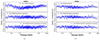 |
Fig. 1. XMM-Newton EPIC-pn pattern-0 data−model residuals from the X-ray spectral fitting using the models described in Sect. 3.1. Left: Bright state observation XMM2 (2008). Right: Faint state observation XMM4 (2019). Significant improvement in the residuals can be seen in both of the multicomponent models, M2 and M3, compared to the single power-law model, M1. |
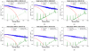 |
Fig. 2. Unfolded best-fitting models for the XMM-Newton EPIC-pn pattern 0 and Suzaku XIS-0 data. The spectral model is the best-fitting, physically motivated model M3 (Sect. 3.1). Solid curves: model evaluated at best fit value; dotted curves: model evaluated at the upper limit; blue markers: unfolded data; red curve: soft X-ray excess modeled by compTT; magenta curve: hot-corona power law; green curve: uxclumpy torus reflection model; black curve: the total unfolded X-ray spectrum. Panels (a), (b), and (c) show bright-state spectra; panels (d), (e), and (f) are for the faint state. These plots illustrate how all X-ray spectral components drop significantly in flux. The strongest drop is for the soft excess, which ultimately disappears in 2021. |
Best parameter estimates obtained from BXA fits to the XMM-Newton and Suzaku datasets.
Henceforth, we adopt the M3 model fits for estimation of the continuum properties of the X-ray spectra. We plot the flux variability of all M3 model components in Fig. 3.
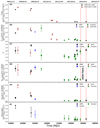 |
Fig. 3. Overview of UV and X-ray spectral components. (a) De-reddened and host-galaxy subtracted UVM2 flux from combined XMM-Newton OM and Swift UVOT data. (b) Integrated total hard X-ray flux. (c) Photon index (Γ) of the hot corona power law (zpowerlwin M3; Sect. 3.1). (d) Integrated flux of the soft excess flux component (0.3–2.0 keV). (e) Integrated flux of the reflection component (2.0–10.0 keV). (f) Integrated Fe Kα emission line flux. Black-circular points: XMM-Newton; brown triangular points: Swift; blue diamond point Suzaku; and green square points: Chandra. The red vertical lines mark the beginning and end of the 2020 outburst in the optical band (Brogan et al. 2023). |
3.2. Chandra X-ray spectral analysis
We applied the inferred best-fitting physically motivated continuum model, M3, to all Chandra datasets. We ignored all ACIS data below 0.7 keV since the drop in effective area yields too few counts for reliable constraints on soft excess model parameters, and we fit up to 8.0 keV. We fixed the compTT temperature (kBT) at 0.17 keV, the optical depth (τ) at 20, while the normalization (AcompTT) was kept free. Observations C6 and C7 were taken within a day, so we fit both datasets simultaneously, allowing only a variable normalization factor between them. The average flux of C6 and C7 is reported in Table 3 and plotted in all flux light curves presented in this paper.
3.3. Swift X-ray spectral analysis
For the Swift-XRT datasets we used data in the 0.3–8.0 keV range. We applied the inferred best-fitting physically motivated continuum model, M3, to the bright state Sw1 and Sw2 datasets to infer spectral properties (e.g., Γ) and individual spectral component fluxes. The soft excess optical depth was kept frozen at τ = 20 for both cases. Best-fitting values for soft excess temperature were  keV for Sw1 and <0.16 keV for Sw2. The low count (<300) intermediate state spectra: Sw3, Sw4, and Sw5, were fit with only a power law to evaluate total model flux.
3.4. The Fe Kα line
The isolated Fe Kα line flux cannot be derived from the M3 model fitting, as the publicly available UXCLUMPY reflection model does not provide a separate component for the Fe Kα emission line. Therefore, we adopted a phenomenological approach, applying a model Mcont + TBabs*Σizgaussi, where Mcont is an underlying continuum and zgauss are the emission line component(s). For neutral or moderately ionized gas, Fe Kα line emission is accompanied by Fe Kβ (7.06 keV rest frame). Due to the close energy proximity of these lines, we accounted for the potential flux contribution from the Fe Kβ line even though it was unresolved due to insufficient counts. We thus added a Gaussian component with width σ tied to that for Kα and normalization tied to 13% (Palmeri et al. 2003) that of the Kα line.
For the high-count spectra, XMM2, SUZ, XMM3, XMM4, and XMM5, we adopted M2 for the continuum component Mcont (Sect. 3.1). Given the substantial proportional uncertainties (up to 32%) in the hard photon indices (Table 2), we freeze Γ1 and Γ2 to the values derived from the continuum fit (Sect. 3.1). Meanwhile, the Gaussian width σFe Kα, its normalization, and the normalization values of the two power laws A1 and A2) are allowed to vary. We kept the Gaussian line centroid frozen at 6.4 keV (rest frame) for all XMM-Newton datasets though not for the Suzaku dataset, where keeping line centroid free returned a better fit.
For the Chandra datasets, we adopted a power law as the underlying continuum. In all fits except for C2 and C6 + C7, we kept the line centroids and widths frozen to 50 eV. For C2, we kept both the width and centroid free, and for C6 + C7 we kept only the line centroid free (Table 3).
We used the Monte Carlo simulations simftest to calculate the detection probability of the Fe Kα line. For all XMM-Newton and Suzaku observations, we obtained a detection probability greater than 99% except for the XMM1 spectrum. The Fe Kα line was detected at high confidence (>95%, with the significance reaching >99% confidence in C2 and C6 + C7) in nearly all Chandra observations except C1 and C8. We list the Fe Kα line parameters, including the equivalent width relative to the local continuum, in Table 3 and plot the Fe Kα flux in Fig. 3.
3.5. Broadband SED analysis
The multi-band behavior of the Mrk 1018 is constrained by the joint fitting of the optical, UV, and X-ray observations. We fit all the high S/N XMM-Newton EPIC-pn and OM datasets using a broadband spectral model; we also included Sw2 in the fit to XMM2. The broadband spectral model consists of a host galaxy template (Mannucci et al. 2001), AGN disk + corona emission from agnsed (Kubota & Done 2018), and distant reflection modeled with uxclumpy, mathematically written as: Magnsed= redden*TBabs*(host_galaxy + agnsed + uxclumpy_reflect). The redden and TBabs components account for the Galactic absorption in the optical/UV and X-ray bands, respectively. For Mrk 1018, E(B−V) = 0.0272 (Schlegel et al. 1998), and the comoving-distance is d0 = 182 Mpc. Furthermore, we always keep the following agnsed parameters: hot corona temperature kBTe = 200 keV, corona height(hx) = 10 Rg, outer radius Rout set to the self-gravity radius (Kubota & Done 2018, and references therein), black hole mass MBH = 107.9 M⊙ (McElroy et al. 2016), θi = 45°, and black hole spin a = 0. The model setup considered X-ray reprocessing in the accretion disk. The broadband spectra of Mrk 1018 contain a significant amount of host galaxy flux relative to the AGN, as indicated by the optical images and spectra in McElroy et al. (2016) and Brogan et al. (2023). The XMM-Newton OM observations did not take data at V and B bands, necessary for optimal constraints on the host galaxy contribution to the SED. Therefore, we kept the host galaxy normalization frozen at the host galaxy level obtained from the optical bands via joint spectral-fitting of the multiwavelength XMM2 and Sw2-UVOT observations from 2008. The host galaxy fraction is just (Fhost galaxy/Ftot) = 4.78×10⁻³ in the UVM2 (4.25–6.81 eV) band. Consequently, the host galaxy has a flux density of Fgal,UVM2 = 6.98×10⁻¹⁷ ergs cm−2 s−1 Å−1 in the UVM2 band. For XMM5, we demonstrated in Sect. 3.1 that the warm coronal component is not robustly detected. Thus, for fitting the XMM5 data in the agnsed framework, we do not include such a component. We report the best-fit values in Table 4, plot the best-fit spectra in Fig. 4, and interpret the results in Sect. 4.4.
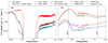 |
Fig. 4. Broadband SED fits using the agnsed model. (a) Absorbed total broadband model. The circular markers indicate XMM-Newton EPIC-pn+OM datasets for the XMM3, and XMM5 observations and XMM-Newton EPIC-pn + OM + Swift-UVOT datasets for XMM2. The solid lines of corresponding color represents the best-fit total models. The XMM1 and XMM4 data points are not plotted for clarity. For XMM3 and XMM5 the OM photometric points almost overlap with each other since they have almost equal fluxes. (b) Corresponding unabsorbed agnsed models. They indicate the significant changes occurring in the intrinsic spectrum, within both the bright and faint flux states. The dashed lines indicate energies used to calculate the optical-X-ray spectral index αOX. |
As a caveat, we bear in mind that the application of the AGNSED model in the faint state is approximate, as the faint state is potentially dominated by an ADAF. Thus, it can have additional radiative contributions from synchrotron, cyclotron, and bremsstrahlung (Narayan & Yi 1995) processes. This additional emission can modify the broad band spectral shape; however, an alternative broad band model that incorporates these radiative processes added to the baseline radiation from the AGNSED model is currently not available. This additional radiative contribution if present can potentially influence our estimates of the model-dependent parameters, for example, Rhot, Rwarm, Γwarm, kTwarm. However, our estimate of the αOX and Eddington ratio are only mildly dependent on spectral modeling and will potentially remain unaffected.
3.6. Continuum X-ray and UV flux variability modeling
To visualize and quantify the variability of the long-term flux drop flong(t), we fit the X-ray and UV data with a phenomenological “modified reverse sigmoid” (MRS) function:
 (1)
(1)
The description of the parameters are the following: Ffaint is the average flux in the faint state; R is the ratio of the bright to the faint state flux; t0 is defined such that  ; and tsc is the timescale quantifying how fast the flux drops, a smaller value implies faster drop. The average long-term flux drop is well captured by the analytical model (Fig. 5). Best-fitting values of R were 7.9 ± 0.5 and 28 ± 2 for hard X-rays (2–10 keV) and UV, respectively; t0 was found to be MJD 56228±195 for X-rays and 55453±245 for UV. Best-fitting values of tsc were 274±187 days for X-rays and 422±109 days for UV, with their mean around 1 year. The quantity
 ![Mathematical equation: $ \left [\frac {R}{t_{\mathrm {sc}}}\right ] $](/articles/aa/full_html/2025/07/aa54707-25/aa54707-25-eq113.gif) quantifies the rate of flux drop; best-fitting values for the X-ray and the UV light curves were
quantifies the rate of flux drop; best-fitting values for the X-ray and the UV light curves were  day−1 and
  day−1, respectively. As a caveat, we note that sparse sampling between 2014 and 2016 can impact our estimates of t0, tsc, and
 ![Mathematical equation: $ \left [\frac {R}{t_{\mathrm {sc}}}\right ] $](/articles/aa/full_html/2025/07/aa54707-25/aa54707-25-eq116.gif) . Additionally, uneven sampling between the X-ray and UV bands, means that we cannot exclude that both bands dropped simultaneously with the same slope. An additional impact is the short-term stochastic variability observed at all flux states of the source.
. Additionally, uneven sampling between the X-ray and UV bands, means that we cannot exclude that both bands dropped simultaneously with the same slope. An additional impact is the short-term stochastic variability observed at all flux states of the source.
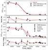 |
Fig. 5. (a) Light-curve data of UVM2 and best-fit MRS function normalized by the faint state flux. (b) Corresponding UVM2 residual. (c) Data of the 2–10 keV X-ray light curve and best-fit normalized by the faint state flux. (d) Corresponding X-ray residual. The circular, diamond, triangular, and the square markers represent XMM-Newton, Suzaku, Swift, and Chandra datasets, respectively. The red line indicates the best-fit MRS model. |
We searched for lags or leads between the 2–10 keV and UVM2 band flux light curves using the interpolated correlated function (ICF; White & Peterson 1994; based on Gaskell & Sparke 1986). To estimate uncertainties, we consider random subset selection and flux randomization following Peterson et al. (1998). The pair of light curves are highly correlated but with no evidence for lags or leads in either case, with lags consistent with zero. For lags from 2–10 keV to UVM2, we find a maximum correlation coefficient rcorr = 0.962 at a delay of τ=−640±962 days, i.e. consistent with zero lag.
4. Results and discussion
4.1. Summary of main results
Previous X-ray studies of Mrk 1018 have generally used rather simple models to quantify its complex X-ray spectrum and spectral behavior. A single power law (Lyu et al. 2021), double-power law (Brogan et al. 2023), and/or a power law + Comptonization model (nthcomp, Zdziarski et al. 1996 in Veronese et al. 2024) have been applied to characterize the X-ray continuum. Here, we fit all high S/N X-ray spectra with a physically motivated three-component model that incorporates the primary hot coronal X-ray power law, a warm Comptonization soft X-ray excess, and a reflection component, including a narrow Fe Kα line.
Our X-ray spectral decomposition demonstrated that the soft excess flux drops by a factor of ∼12 compared to bright-state across all observations, along with significant short term variability through the entire period of its detection until 2019. However, despite this strong flux drop, the parameters of the warm corona (optical depth τ, electron temperature kBTe) do not evolve significantly through the entire period of its detection until 2019. Ultimately, the soft excess was not detected anymore in the high-count XMM-Newton spectrum in 2021.
Meanwhile, the hot corona photon index Γ demonstrates distinct trends: first decreasing across the bright-to-faint transition, and then increasing again after roughly 2018, when Mrk 1018 was in the faint state. These trends are discussed below in more detail.
The UV-to-X-ray emission can be modeled with the thermal Comptonization model agnsed, and best-fitting X-ray parameters (e.g., kBTe) are generally consistent with the best-fitting M3 models to the X-ray-only data. Similarly, agnsed does not return a soft-X-ray excess contribution for XMM5, consistent with the X-ray-only fitting (Fig. 4). We characterize the broadband spectral evolution using the UV-X-ray spectral index αOX (Tananbaum et al. 1979). Values are listed in Table 4. αOX decreases from XMM1 to XMM3, but then increase through XMM4 and XMM5; a similar trend is also seen in the hot-corona powerlaw X-ray photon index (Γ).
All emission components dropped in intensity during the spectral transition but by differing factors. To quantify these differences we examine the overall evolution in broadband spectral shape from the bright state to the faint state. We define a ratio spectrum, R(E), to indicate the ratio of the flux density in the bright state to that in the faint state. R(E) is determined from the average best-fitting model parameters for three spectra in each state, as detailed in Appendix B. We plot R(E) as a function of energy in Fig. 6. The strongest contributors to evolution of the broadband spectral shape are the UV-band and the soft X-ray band. The average fluxes for each spectral component in the two states are listed in Table 5.
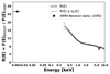 |
Fig. 6. Energy resolved bright and faint state flux ratio. The solid black line is the ratio of the average X-ray spectra (R(E)) in the bright and the faint phase and the dashed lines demarcate the upper and lower error. The plot is based on the M3 model compTT + zpowerlw + uxclumpy-reflect calculated for the high-count XMM-Newton and Suzaku spectra. The UVM2 flux ratio (diamond marker) is derived from XMM-Newton OM observations. |
Average flux of the UVM2 (5.32 eV) band, X-ray spectral components, and bolometric luminosity with their respective flux drop.
Comparing the flux drops across the Fe Kα line, the hard X-ray power law, the soft excess, and the UV luminosity (Table 5), defined as RFe Kα, RHX, RSX, and RUVM2, respectively, we note that RFe Kα < RHX < RSX < RUV, roughly consistent with the shape of the broadband R(E) curve in Fig. 6. The results suggest that there is an overall broadband spectral hardening due to the CLAGN transition from the bright to faint state, which results from the interplay between different spectral components and bands. However, individual spectral components exhibit divergent behavior as described in the subsequent sections.
4.2. The warm corona in Mrk 1018
Mrk 1018 exhibits a drastic drop in the flux of the soft X-ray excess – a factor of 12 between the average bright and faint states (Table 5). In the context of the warm Comptonization model (e.g., Boissay et al. 2016), however, there is no systematic change in the warm corona parameters through the entire period of its detection until 2019. We find that the temperature is always in the range 0.13 keV <kBTe< 0.2 keV and opacity values are optically thick with τ>10, which are consistent with studies by Mehdipour et al. (2011), Petrucci et al. (2013), Ballantyne et al. (2024), Palit et al. (2024). One possible explanation for the decrease in soft excess until 2019 in the context of warm Comptonization is that due to the decrease in λEdd, fewer optical/UV thermal seed photons from the accretion disk are incident on the warm corona. We note that values of FSX,compTT/Ftot, as listed in Table 2, very roughly linearly track the corresponding values of λEdd. This scenario does not need to invoke any changes in the structure or properties of the warm corona during that process.
On the other hand, during the faint state, other physical processes seem to be active. From XMM3 (2018) to XMM4 (2019) and XMM5 (2021), the soft excess contribution decreased by at least a factor of ∼3. Since the soft excess component was not detected in the high S/N XMM5 data from 2021, its upper limits indicate only another decrease by a factor of ∼2 compared to XMM4. In the same time (between XMM3, XMM4, XMM5), the UV seed photon emission varied only by ≲30% (Tables 3, 4 and Fig. 4). Interestingly, XMM3 and XMM5 even have very similar UVM2 flux levels. Thus, it is unlikely that the further soft excess decrease below our detection limit (or its disappearance) after 2019 is driven solely by the variation in accretion disk seed photons. Since the seed photon production does not change significantly in the faint state, an alternate plausible explanation is a delayed (with respect to the time of CLAGN detection) structural change, disintegration, or disappearance of the warm corona (producing the soft excess). This notion is supported by the SEDs of samples of unobscured Seyferts studied by Hagen et al. (2024) in the context of the geometry assumed in the agnsed model. The radiatively efficient inner flow along with the warm corona becomes absent for λedd≲0.02. This results in the negligible interception of cooler accretion disk seed photons in the faint state. The exact mechanism of warm corona disintegration or disappearance is still unknown. However, it has been proposed that with the decrease in accretion rate, the flow transforms into a radiatively inefficient advection dominated accretion flow (ADAF; Narayan & Yi 1995; Esin et al. 1997) and subsumes the radiatively efficient components of the accretion flow.
Multiple other sources also exhibit extreme soft excess variability tied to rapid accretion rate changes. Recent studies of the CLAGN NGC 1566 report the appearance of a strong Comptonized soft excess during a high-accretion state and its significantly weaker or negligible presence during a low-accretion state over a time span of ∼3 years (Jana et al. 2021; Tripathi & Dewangan 2022). Similar trends are also exhibited by the flaring CLAGN LCRS B040659.9−385922, detected with eROSITA, (Krishnan et al. 2024) where the soft excess strengthened during the rise and faded during the decay of a ∼1.4 year flare. Overall, the soft excess in these transient individual CLAGN sources, including Mrk 1018, exhibits a direct correlation of the soft excess’ intensity with an extremely variable accretion rate (λEdd).
An alternate, although speculative, explanation of the disappearance of the warm corona and soft excess could be the destruction of the warm corona, driven by the strong optical outburst observed in 2020 (Brogan et al. 2023; Lu et al. 2025). However, we would need additional X-ray spectral studies of Mrk 1018 in the near future to adequately test if the soft excess has returned or remains absent and thus to illuminate the connections between the presence or disappearance of the warm corona, the long-term accretion rate changes, and the potential impact of the 2020 outburst. We note a partially analogous situation to that in the CLAGN 1ES 1927+654 (Trakhtenbrot et al. 2019), where the hot corona was temporarily destroyed by an extrinsic event, possibly due to the impact of a tidally disrupted star (Ricci et al. 2020).
4.3. The inner hot flow in Mrk 1018
The hot Comptonized X-ray emission in Seyferts and black hole X-ray binaries (BHXRBs) is proposed to originate from a hot-inner accretion flow, either in a compact X-ray corona (Haardt & Maraschi 1991, 1993) or an advection dominated flow (Ptak et al. 1998) through upscattering of UV or optical seed photons. The seeds originate primarily from the optically thick accretion disk (e.g., Kubota & Done 2018).
A softer-when-brighter trend for accretion rates above log(λEdd)∼−2 has been noted in samples of Seyferts as well as in individual BHXRBs (e.g., Lusso et al. 2010). Meanwhile, at lower accretion rates, a softer-when-fainter behavior has been recorded for samples of low-luminosity AGNs (Gu & Cao 2009; Younes et al. 2011; She et al. 2018) and in individual BHXRBs (e.g., GRO J1655−40, Sobolewska et al. 2011) in their low-hard state (Wu & Gu 2008; Yang et al. 2015). We plot the hot corona photon index (Γ) versus Eddington ratio (λEdd) for Mrk 1018 in Fig. 7. While in the bright phase the scatter in the data points does not reveal any trend. However, Mrk 1018 exhibits a softer-when-fainter state trend or an anti-correlation in the Γ-λEdd relation (ρcorr=−0.89, p = 1.4×10⁻³) in the faint state after 2016. A linear regression returns the best-fitting relation
 (2)
(2)
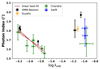 |
Fig. 7. Evolution of the photon index (Γ) of the intrinsic hot corona power law with respect to the Eddington ratio (λedd=Lbol/Ledd). The different colors represent different missions: green, Chandra; red, Chandra observation from 2010 evaluated from readout streak; blue, XMM-Newton; orange, Suzaku; brown solid line, linear regression best-fit in the softer-when-fainter state; brown dashed line, the uncertainty range of the linear fit. The soft-when-fainter trend is evident for log λEdd<−1.7. |
Here, we have used only the high-count data and a physically motivated model (M3), thus reducing the scatter in Γ and the statistical uncertainty. Lyu et al. (2021) have reported this phenomenon in terms of Γ and the X-ray flux (2–10 keV) for the low count Swift-XRT datasets, using only a simple power law fitting. Meanwhile, the UV-X-ray spectral index αOX in Mrk 1018 decreased initially but increased after 2018 (Table 4), a behavior similar to that of Γ. The softer-when-fainter trend in optical-X-ray spectral index (αOX) is seen in samples of low-luminosity AGNs and CLAGNs (e.g., Li & Xie 2017; Ruan et al. 2019). The two convergent trends in Γ and αOX as a function of λEdd observed in individual BHXRBs, samples of CLAGNs and low-luminosity AGNs generally support the notion that a geometrically thin disk dominates the spectrum at Eddington ratio values log λEdd≳ −2, whereas an ADAF dominates the accretion structure at values of log λEdd≲ −2, respectively (e.g., Sobolewska et al. 2011; Ruan et al. 2019). It would seem that the innermost accretion structure in Mrk 1018 also underwent a transition as noted by Lyu et al. (2021) as log λEdd dropped below roughly −1.7 (Li & Xie 2017). The observed timescale for Γ to transition from softer-when-brighter to softer-when-fainter (hereafter tΓ) is thus indicative of (a) the timescale of disintegration or disappearance (e.g., Hagen et al. 2024) of the optically thick inner flow and/or (b) the timescale over which the alternative seed photon source, for example, an ADAF producing synchrotron seed photons (Gu & Cao 2009, and reference therein), dominates. As shown in Fig. 3c, tΓ spans 4–10 years. The large uncertainty on tΓ is due to the large uncertainty on Γ in the 2010 Chandra observation (see Fig. 3c). If the value of Γ had already fallen by 2010, this drop would be remarkable, since it would have occurred before the observed optical CLAGN transition, possibly indicating a precursory change in the accretion flow.
4.4. Multiwavelength connection
Over the bright-to-faint transition from 2010–2013, the UV luminosity flux drops by a factor of ∼24 whereas the X-ray drops by a factor is ∼8 (Table 5). Additionally, the UV integrated model luminosity in the 2–15 eV band contributes a significant fraction to the UV–X-ray SED (Table 4) where LUV/(LUV+LX−ray)∼0.6–0.7 in the bright phase and ∼0.5 in the faint state, with LUV>LX−ray for most broadband spectrum, similar to most Seyferts accreting at log λEdd∼−2. Thus, from an energy argument, the larger UV variability-factor and its larger contribution to the total luminosity indicate that Comptonization of the UV seed-photons (Haardt & Maraschi 1991; Haardt et al. 1994) in a hot-corona/accretion flow is more likely to drive long term X-ray variability; as opposed to X-ray driving the UV via thermal reprocessing. This picture is also reinforced by other studies (e.g., Uttley et al. 2003; Hagen & Done 2023) explaining the inadequacy of the X-ray reprocessing in driving large amplitude-long term optical/UV variability in normal non-CLAGN. Additionally, UV emission driving X-ray emission is consistent with the notion that the physical process triggering the CLAGN transition initially affects a region in the accretion flow that primarily emits UV.
Furthermore, there is a non-trivial mismatch between the factors in the drops of UV and X-ray fluxes (RUV≃3RHX; Table 5). If the hot corona is static in morphology and physical properties across the bright and faint states, then the number of UV seed photons intercepted by the hot corona for upscattering to X-rays should decrease by the same factor as the UV flux (Appendix C). In other words, the observed X-rays should also drop by that same factor. However, the X-rays drop by a much lower factor, (RHX) indicating that the drop in the number of seed photons is partially compensated by an increased level of Comptonization, and/or by other radiative processes in the faint state. Such a situation can be achieved if the inner hot Comptonizing accretion flow becomes relatively more energetically dominant by (a) increasing its covering factor by a factor of three, thus intercepting a higher fraction of seed photons in the faint state (three times more) than in the bright state, albeit with a lower total X-ray luminosity, (b) increasing in the energy imparted per electron and seed-photon scattering due to a hotter corona or ADAF in the faint state, and/or (c) increasing the X-ray emission due to other radiative processes that may occur in radiatively inefficient flows, such as synchrotron, cyclotron, and/or bremsstrahlung emission (Narayan & Yi 1995).
All these observations – the severely reduced UV luminosity in the faint state, the value of RHX being less than that of RUV, the disappearance of the soft X-ray excess, the inversion of the Γ−λEdd relation as noted in this work and in Lyu et al. (2021) – support the scenario in which a switch occured between two accretion configurations (following Esin et al. 1997 for BH XRBs; see also Lyu et al. 2021 for Mrk 1018). Specifically, in the bright state, a geometrically thin, optically thick, UV or optical-emitting disk is present (Fig. 8a), supplying seed photons to both a hot hard X-ray-emitting flow and a warm soft excess-emitting corona for X-ray production. In the faint state, the geometrically thin disk retreats to larger radii. Meanwhile, the inner hot flow or ADAF increases its presence spatially and energetically (Fig. 8b), yielding a higher covering fraction to intercept more seed photons for Comptonization, and/or producing more emission via other processes – synchrotron, bremsstrahlung, etc. If this scenario holds, the UV band should also increase more significantly than the X-ray band if Mrk 1018 switches back to its bright state configuration in the future.
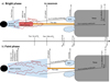 |
Fig. 8. Illustration of one possible geometrical change in AGN accretion structures due to the major CLAGN transition occurring after 2013. Length scales as illustrated here are approximate only. (a) Bright state configuration: warm corona present in the inner accretion structure along with the hot-accretion flow or corona or less dominant ADAF. (b) Faint state configuration after ∼2021: warm corona disappears (Sect. 4.2) and the inner accretion flow becomes dominated by a hot ADAF (Sect. 4.3), emitting X-rays and UV seed. The thin disk also decreases its energy contribution and physical size. Finally, the broad line region (BLR) + torus system extends from sub-parsec scale to 10 s of parsecs, which results in significant smoothing of the Fe Kα line response (Sect. 4.6.1 and Fig. 9). |
4.5. Variability timescales and driving mechanism
Variability in an accretion disk can be characterized by multiple timescales (Frank et al. 2002). The dynamical timescale is given by  . The thermal and viscous timescales are given by tth=(1/α)tdyn and tvisc=(H/R)−2tth, respectively. These timescales are dependent on the radial distance (R), the disk aspect ratio (H/R), and viscosity parameter (α, Shakura & Sunyaev 1973). By estimating these timescales and comparing them with variability timescales measured in Mrk 1018, we can speculate on the possible origin(s) of the source's extreme variability.
The observed timescales associated with the long-term CLAGN transition of Mrk 1018 are (a) tbright≃30 years, the observed time through which Mrk 1018 maintained its bright state (optical type 1), and (b) tsc≃1 year (Sect. 3.6), the transition timescale, which quantifies how fast the broadband flux drops after roughly MJD 55500–56200, eventually leading to the latest optical type transition.
Assuming a black hole mass of MBH = 107.9 M⊙ (McElroy et al. 2016), radial distance values of R = 50–100 Rg in the accretion flow, a viscosity value of α = 0.01, and disk aspect ratio of H/R = 0.001 (thin disk), we obtain dynamical timescales of tdyn≃1.6–4.6 days, thermal timescales of tth≃0.44–1.24 years, and viscous timescales (for a geometrically thin disk) of tvisc≃ 180–500 years, respectively. The thermal timescale is thus consistent with our measured value of tsc. However, neither tth nor tvisc for a geometrically thin disk are consistent with tbright. If we increase the disk aspect ratio (H/R) to 0.2, then the viscous timescales (tvisc) get reduced to 10–30 years, consistent with the observed value of tbright. Our work is consistent with previous suggestions that geometrically thick disks are compatible with observed CLAGN transition timescales, e.g., Dexter & Begelman (2019) for magnetic pressure-supported disks.
The observed timescales of Mrk 1018's transition can also be qualitatively explained in the context of disk instability models. The inner region of the accretion flow in an AGN is typically dominated by radiation pressure (e.g., Laor & Netzer 1989; Noda & Done 2018), resulting in an instability (Lightman & Eardley 1974; Noda & Done 2018; Sniegowska et al. 2020). The instability heats the disk (Lightman & Eardley 1974), increasing the disk aspect ratio (H/R, a geometrically thicker flow as proposed above) on the thermal timescale (∼tth), and the bright state, with an elevated accretion rate, begins. The bright state then sustains for a time period of tbright, explained by a reduced viscous timescale. The instability ends, and the disk reverts to its faint state on a thermal timescale (tth), thus explaining the observed value of tsc. To summarize, an intrinsic instability in the inner accretion flow can thus self-consistently explain the timescales connected to the drastic flux drop between 2010 and 2012 and consequently the optical type transformation detected in 2016. Our proposed mechanism of the CLAGN transition exploits the fact that the above mentioned disk instability process can induce a long term extreme variability flare intrisically, which is a parallel alternate to extrinsic driving mechanism such as chaotic cold accretion (Gaspari et al. 2013, 2017, 2020) as described by Veronese et al. (2024).
In addition to its long term variability behavior, Mrk 1018 exhibited two brief outbursts in 2016 (Krumpe et al. 2017) and 2020 (Brogan et al. 2023), each lasting ≲1 year. The disk radiation-pressure instability scenario can also explain these relatively shorter timescales, as ranges of various model parameters (e.g., Fig. 4 of Sniegowska et al. 2020) can yield extreme variability flares of various timescales. However, we argue that the dominant changes in the structure and energetics of the inner accretion flow (Sect. 4.4) are primarily driven by the 30 year-long bright state, as it has generated at least 25 times more energy than the two year-long outbursts (Appendix D).
4.6. The Fe Kα emission line
4.6.1. Origin
The Fe Kα line in AGNs can either originate in the inner accretion flow, strongly broadened under the influence of the black hole's gravity (e.g., Fabian et al. 1989, 2000) and/or in the distant matter such as the broad line region (BLR) (e.g., Bianchi et al. 2008) or the parsec-scale torus (e.g., Ricci et al. 2014a), consequently yielding a narrow core.
We estimated the constraints on the Fe Kα line width (Table 3) and thus constraining the inner radial bound of its origin. Our Gaussian modeling of the Fe Kα (Sects. 3.4 and 3.2) shows that the emission line has an average width of  eV over all phases. Assuming Keplerian motion (R=GMBH/v2), the FeKα line width yields an inner radius value in the range 0.002–0.08 pc.
In samples of unobscured and mildly obscured Seyferts (e.g., Yaqoob & Padmanabhan 2004; Shu et al. 2010), the narrow Fe Kα line emission can be localized to the outer accretion disk or BLR, using Chandra HETG. In NGC 4151, Fe Kα profile decomposition using high-resolution spectroscopy (Xrism Collaboration 2024) yields that a significant fraction of the Fe Kα line flux originates from gas commensurate with the BLR. Furthermore, reverberation mapping studies for NGC 4151 and NGC 3516 (Zoghbi et al. 2019; Noda et al. 2023) also infer Fe Kα line-emitting gas to be commensurate with the BLR. The torus also contributes a narrow line core and a Compton shoulder (Yaqoob 2012; Xrism Collaboration 2024) to the line profile. From the continuum estimates obtained from our broadband SED (Sect. 3.5) and the radius-luminosity expressions of Bentz et al. (2013) and Kaspi et al. (2007), we obtain an estimate for the BLR size of ∼0.03 pc and ∼0.01 pc in the bright and faint state, respectively. This estimate is also consistent with the average BLR distance estimate of 0.02–0.05 pc from McElroy et al. (2016) and Lu et al. (2025). The dust-sublimation radius for Mrk 1018 was estimated to be ∼0.1 pc (faint state) by (Brogan et al. 2023; Lu et al. 2025). Thus, the range of the inner radius obtained from the Fe Kα line width overlaps with the range demarcated by the BLR distance estimate and the dust-sublimation radius of Mrk 1018.
4.6.2. The extent of the Fe K α line emitting region
The most likely explanation for the observed mismatch between the flux-drop factors of the emission line, RFe ∼ 3.4, and its driving continuum, Rion,Fe = 6.8, is that the Fe Kα line has not fully responded yet to reach its expected faint-state flux, which should be Ffaint(Fe Kα) =Fbright(Fe Kα)/Rion,Fe. We model and interpret these drops in flux using a phenomenological reverberation model. In this model, a bi-conically cutout reprocessor (a commonly used geometry in torus modeling, e.g., Ikeda et al. 2009; Baloković et al. 2018) is illuminated by an ionizing continuum originating from a central X-ray point source. Our numerical scheme adds up the response from the different volume elements accounting for time-delays. We assumed a static inner radius of Rin = 0.01 pc (consistent with a BLR) and opening angle θo = 45° and estimated the radial extent (outer radius Rout) of the reprocessor that is required to smear and smooth the observed Fe line response of an ionizing continuum (Fion(t) fit by the MRS function; Sect. 3.6). We fit the Fe Kα observed light curve re-normalized with its plausible type 1.9 flux (Ffaint(Fe Kα)) with our model predicted light curve. This returns an optimal value of  pc (Fig. 9). This estimate is consistent with the estimate that the infrared torus extends from sub-parsec distances to distances up to ≲100 pc (Hönig et al. 2013; Hönig & Kishimoto 2017; Hönig 2019). Thus spatial extent of the Fe Kα emitting torus indicates, that the iron emission line would require about additional ∼9 years from now to fully respond to the flux drop that occurred between 2010 and 2012 and settle to the faint state value. Detecting this drop will require high S/N monitoring of the source over the next decade.
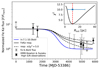 |
Fig. 9. Response of an extended parsec-scale structure with inner radius of Rin = 0.01 pc line response and outer radius Rout = 10 pc. The dashed lines correspond to the upper and lower errors of Rout. Inset: Reduced-χ2 from the Fe Kα light-curve fit best estimate of the external radius. The blue marker and red dashed line represent the best-fitting value, and the error bar corresponds to Δχ2 = 5. |
This estimate of the outer radial extent of the iron line emitting region comes with a few caveats: (a) Our constraints on the inner radius (Rin) are limited by CCD energy resolution, whereas high-resolution measurements are offered only by gratings and calorimeters. (b) There can potentially be some Compton scattering in relatively cold material of BLR or torus that might result in Compton-shoulders (e.g., Yaqoob & Murphy 2011; Buchner et al. 2019), consequently affecting line width when modeling it with a single Gaussian. (c) The response of the Fe Kα echo from a distant structure is based on a single scattering of the incident beam and does not take into account detailed radiative transfer effects. (d) The Fe Kα flux from XMM5, which is included for the above analysis, was taken immediately after the short 2020 outburst and might have minimal influence on the constraints obtained from long term trends.
Despite the limited dataset and the caveats mentioned above, we determined a reasonable estimate of the maximum path length covered (Δr∼10 pc) by an ionizing continuum photon in the line emitting medium, indicating that a physically extended region (outer BLR to the parsec scale torus) likely acts to smear out the emission line response to the variable continuum. Additionally, our modeling strengthens our hypothesis that as of 2021, the Fe Kα line has not undergone a full decay, and is still responding to the abrupt CLAGN ‘shutdown’ event after 2013.
4.6.3. Equivalent width and the line profile
The Fe Kα line in Mrk 1018 exhibits flux variations (Fig. 10), which consequently affects its equivalent width (EW). A systematic increase in EW (excepting the 2016 observation) is observed as the flux drops. The trend exhibits a Pearson's correlation coefficient of ρcorr=−0.62 (p = 0.03), indicating a mild anti-correlation. Such an anti-correlation is observed across multiple samples of type 1 and type 2 AGNs (e.g., Iwasawa & Taniguchi 1993; Shu et al. 2012; Ricci et al. 2014b; Boorman et al. 2018). The drivers of evolution in EW can be associated with two distinct physical processes: (a) variation of the underlying continuum (Jiang et al. 2006) and/or (b) variation of the covering fraction of distant narrow line-emitting material (Page et al. 2004) due to increasing radiation from the central engine (Ricci et al. 2017). In this case, the Fe Kα line originates in the sub-parsec BLR and/or the torus. Thus, a more relevant mechanism is the BLR covering fraction change induced by variations in Lbol on the thermal timescale (tth). For our case, at R = 0.01 pc (Sect. 4.6.1), tth is as high as 160 years. Thus, our observed mild anti-correlation of Fe Kα to the X-ray continuum does not result from the covering fraction change in the BLR or torus. The most plausible cause of the generic trend of EW variation is the slower drop of the Fe Kα flux relative to the continuum X-ray flux.
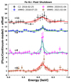 |
Fig. 10. Spectral fits to the Fe Kα line from C2 (2016), XMM3 (2018), XMM4 (2019), and XMM5 (2021; datasets are grouped for clarity). The dashed lines indicate the profile corresponding to the upper and lower error bars of σFeKα. The spectra have been normalized using the underlying continuum model. The relative strength or intensity of the Fe Kα line with respect to the continuum is significantly highest for C2 and XMM5 and lowest for XMM3. |
Considering observation C2, the Fe Kα EW width exhibits a significant increase from pre-shutdown levels, ∼100 eV, to 464 ± 200 eV in 2016 (Fig. 11), a distinct deviation from the long term increasing trend. We could not assign a particular cause to the sudden increase in EW in the C2 spectrum, except stochastic variability of the underlying continuum.
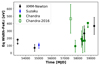 |
Fig. 11. Time evolution of Fe Kα equivalent width, which exhibits a mild increase with time. Black circular markers: XMM-Newton; blue diamond marker: Suzaku; unfilled green square marker: Chandra from 2016 (C2); green square markers: all other Chandra spectra. |
5. Summary and conclusions
Mrk 1018 is part of the rare class of CLAGNs that have exhibited multiple extreme variations in luminosity and optical spectral type transition. In the 1980s, Mrk 1018 transitioned from type 1.9 (faint state) to a type 1.0 (bright state; Cohen et al. 1986). It remained in this bright state for roughly 30 years, after which it reverted to a type 1.9 (faint state) in the early 2010s (McElroy et al. 2016; Husemann et al. 2016).
We analyzed the long-term multiwavelength properties of the source (across 2003–2021), with a focus on the behavior during the transition from the bright state to the faint state, which started roughly between 2010 and 2013. In particular, we modeled all available high S/N X-ray spectra with a physically motivated multicomponent model, and we quantified the broadband SED variability behavior. We established the following characteristic changes in the inner accretion flow due to the CLAGN transition:
-
The soft excess became fainter through 2019, maintaining temperatures between 0.1 and 0.2 keV and optical depths between 10 and 30. However, the soft excess was not detected in the high S/N 2021 faint-state spectrum. It is possible that during the faint state, the warm corona structurally disintegrated or became energetically negligible by 2021, likely driven by the overall decrease in the accretion rate. Alternatively, the deficit of soft excess emission might simply be time-localized, driven by some disruption resulting from the 2020 optical/UV outburst.
-
The hot corona photon index (Γ) when plotted against λEdd follows a softer-when-fainter trend in the faint state (log λEdd≲10−1.7), as determined by the high-quality spectra (Eq. (2)). Our results are consistent with the Γ–LX−ray trends obtained from the fitting of low S/N data by Lyu et al. (2021) and those observed in some BHXRBs and samples of low-luminosity AGNs.
-
The broadband spectrum from UV to X-rays hardened during the transition from the bright to the faint state, as different emission components responded differently. The UV emission dropped by a factor that is three times greater than the corresponding drop in the hard X-ray emission.
-
The substantial drop in UV emission during the transition and the inverted Γ–λEdd relation observed during the low state are consistent with the CLAGN transition being driven by structural changes in the inner accretion flow. Specifically, the inner geometrically thin disk transforms into a hot ADAF. The observation that the hard X-ray flux from the hot corona drops by a factor lower than the UV thermal disk emission could be explained by either an increased covering fraction of the ADAF or increased contributions from other X-ray continuum emission processes associated with ADAFs, such as synchrotron or bremsstrahlung.
-
While the Fe Kα line flux is driven by variability in the hard X-ray continuum, the Fe Kα line and the ionizing continuum exhibit significantly different variability factors. The observed line width and simple reverberation modeling constrain the extent of its emitting region to be between 0.01 pc and a few tens of parsecs.
-
Furthermore, we predict that the Fe Kα line has not fully responded, as the more distant regions of the line-emitting gas are yet to respond. Simple modeling predicts that it could still require an additional nine years (approximately) from the present for the Fe Kα to settle down to a new equilibrium value.
The complex multiwavelength and multicomponent behavior in Mkn 1018 warrants continued long-term monitoring across the EM spectrum. If the extreme variability observed in Mrk 1018 results from a limit-cycle behavior, then multiple successive short- and long-term outbursts (with a few outbursts already observed) are a possibility. Speculatively, such behavior may also be occurring within the class of objects exhibiting recurrent CLAGN events, and Mrk 1018 may be part of this class (Wang et al. 2025). Studying such outbursts, both in samples and in individual objects, will allow the community to advance theoretical models of accretion instabilities.
Furthermore, integral field or millimeter wave observations (e.g., ALMA) can map out cold circumnuclear structures to allow for testing of whether substantial reservoirs of cold gas remain that can fuel future bright phases. As well, this would allow for further testing on the viability of a chaotic cold accretion model triggering CLAGN transitions.
Acknowledgments
The authors thank the anomymous referee for the comments and suggestions. TS acknowledges full and partial support from Polish Narodowym Centrum Nauki grants 2018/31/G/ST9/03224, 2016/23/B/ST9/03123, and from Deutsches Zentrum für Luft- und Raumfahrt (DLR) grant FKZ 50 OR 2004. MK is supported by DLR grant FKZ 50 OR 2307. AM acknowledges full or partial support from Polish Narodowym Centrum Nauki grants 2016/23/B/ST9/03123, 2018/31/G/ST9/03224, and 2019/35/B/ST9/03944. MG acknowledges support from the ERC Consolidator Grant BlackHoleWeather (101086804). This research is based on observations obtained with XMM-Newton, an ESA science mission with instruments and contributions directly funded by ESA Member States and NASA. This research has made use of data obtained from the Chandra Data Archive provided by the Chandra X-ray Center (CXC). This research has made use of data and/or software provided by the High Energy Astrophysics Science Archive Research Center (HEASARC), which is a service of the Astrophysics Science Division at NASA/GSFC. This research has made use of the NASA/IPAC Extragalactic Database (NED), which is funded by the National Aeronautics and Space Administration and operated by the California Institute of Technology. We acknowledge the use of public data from the Swift data archive. This work made extensive use of the following python packages: NumPy (Harris et al. 2020), Matplotlib (Hunter 2007), SciPy (Virtanen et al. 2020), pandas (Wes McKinney 2010; The pandas development team 2020), and Astropy (Astropy Collaboration 2022).
The family of extreme variability AGNs also includes events associated with variations in line-of-sight X-ray obscuration, e.g., Markowitz et al. (2014, 2024), Serafinelli et al. (2021), Marchesi et al. (2022), Sengupta et al. (2025) and references therein.
 2 implies ‘Mi’ is a better model (Buchner et al. 2014).
References
- Arnaud, K. A. 1996, in Astronomical Data Analysis Software and Systems V, eds. G. H. Jacoby, & J. Barnes, ASP Conf. Ser., 101, 17 [NASA ADS] [Google Scholar]
- Astropy Collaboration (Price-Whelan, A. M., et al.) 2022, ApJ, 935, 167 [NASA ADS] [CrossRef] [Google Scholar]
- Balbus, S. A., & Hawley, J. F. 1991, ApJ, 376, 214 [Google Scholar]
- Ballantyne, D. R., Sudhakar, V., Fairfax, D., et al. 2024, MNRAS, 530, 1603 [NASA ADS] [CrossRef] [Google Scholar]
- Baloković, M., Brightman, M., Harrison, F. A., et al. 2018, ApJ, 854, 42 [Google Scholar]
- Bentz, M. C., Denney, K. D., Grier, C. J., et al. 2013, ApJ, 767, 149 [Google Scholar]
- Bianchi, S., La Franca, F., Matt, G., et al. 2008, MNRAS, 389, L52 [NASA ADS] [Google Scholar]
- Boissay, R., Ricci, C., & Paltani, S. 2016, A&A, 588, A70 [NASA ADS] [CrossRef] [EDP Sciences] [Google Scholar]
- Boorman, P. G., Gandhi, P., Baloković, M., et al. 2018, MNRAS, 477, 3775 [CrossRef] [Google Scholar]
- Brogan, R., Krumpe, M., Homan, D., et al. 2023, A&A, 677, A116 [NASA ADS] [CrossRef] [EDP Sciences] [Google Scholar]
- Buchner, J., Georgakakis, A., Nandra, K., et al. 2014, A&A, 564, A125 [NASA ADS] [CrossRef] [EDP Sciences] [Google Scholar]
- Buchner, J., Brightman, M., Nandra, K., Nikutta, R., & Bauer, F. E. 2019, A&A, 629, A16 [NASA ADS] [CrossRef] [EDP Sciences] [Google Scholar]
- Burrows, D. N., Hill, J. E., Nousek, J. A., et al. 2005, Space Sci. Rev., 120, 165 [Google Scholar]
- Cash, W. 1979, ApJ, 228, 939 [Google Scholar]
- Cohen, R. D., Rudy, R. J., Puetter, R. C., Ake, T. B., & Foltz, C. B. 1986, ApJ, 311, 135 [NASA ADS] [CrossRef] [Google Scholar]
- Denney, K. D., De Rosa, G., Croxall, K., et al. 2014, ApJ, 796, 134 [Google Scholar]
- Dexter, J., & Begelman, M. C. 2019, MNRAS, 483, L17 [NASA ADS] [CrossRef] [Google Scholar]
- Duras, F., Bongiorno, A., Ricci, F., et al. 2020, A&A, 636, A73 [NASA ADS] [CrossRef] [EDP Sciences] [Google Scholar]
- Esin, A. A., McClintock, J. E., & Narayan, R. 1997, ApJ, 489, 865 [NASA ADS] [CrossRef] [Google Scholar]
- Fabian, A. C., Rees, M. J., Stella, L., & White, N. E. 1989, MNRAS, 238, 729 [Google Scholar]
- Fabian, A. C., Iwasawa, K., Reynolds, C. S., & Young, A. J. 2000, PASP, 112, 1145 [NASA ADS] [CrossRef] [Google Scholar]
- Feroz, F., Hobson, M. P., & Bridges, M. 2009, MNRAS, 398, 1601 [NASA ADS] [CrossRef] [Google Scholar]
- Frank, J., King, A., & Raine, D. J. 2002, Accretion Power in Astrophysics: Third Edition (Cambridge, UK: Cambridge University Press) [Google Scholar]
- Gabriel, C., Denby, M., Fyfe, D. J., et al. 2004, in Astronomical Data Analysis Software and Systems (ADASS) XIII, eds. F. Ochsenbein, M. G. Allen, & D. Egret, ASP Conf. Ser., 314, 759 [NASA ADS] [Google Scholar]
- Garmire, G. P., Bautz, M. W., Ford, P. G., Nousek, J. A., & Ricker, G. R. Jr. 2003, in X-Ray and Gamma-Ray Telescopes and Instruments for Astronomy., eds. J. E. Truemper, & H. D. Tananbaum, SPIE Conf. Ser., 4851, 28 [Google Scholar]
- Gaskell, C. M., & Sparke, L. S. 1986, ApJ, 305, 175 [NASA ADS] [CrossRef] [Google Scholar]
- Gaspari, M., Ruszkowski, M., & Oh, S. P. 2013, MNRAS, 432, 3401 [NASA ADS] [CrossRef] [Google Scholar]
- Gaspari, M., Temi, P., & Brighenti, F. 2017, MNRAS, 466, 677 [Google Scholar]
- Gaspari, M., Tombesi, F., & Cappi, M. 2020, Nat. Astron., 4, 10 [Google Scholar]
- Gehrels, N., Chincarini, G., Giommi, P., et al. 2004, ApJ, 611, 1005 [Google Scholar]
- Ghosh, R., Laha, S., Deshmukh, K., et al. 2022, ApJ, 937, 31 [Google Scholar]
- Gu, M., & Cao, X. 2009, MNRAS, 399, 349 [NASA ADS] [CrossRef] [Google Scholar]
- Haardt, F., & Maraschi, L. 1991, ApJ, 380, L51 [Google Scholar]
- Haardt, F., & Maraschi, L. 1993, ApJ, 413, 507 [Google Scholar]
- Haardt, F., Maraschi, L., & Ghisellini, G. 1994, ApJ, 432, L95 [NASA ADS] [CrossRef] [Google Scholar]
- Hagen, S., & Done, C. 2023, MNRAS, 521, 251 [NASA ADS] [CrossRef] [Google Scholar]
- Hagen, S., Done, C., Silverman, J. D., et al. 2024, MNRAS, 534, 2803 [NASA ADS] [CrossRef] [Google Scholar]
- Harris, C. R., Millman, K. J., van der Walt, S. J., et al. 2020, Nature, 585, 357 [NASA ADS] [CrossRef] [Google Scholar]
- Homan, D., Krumpe, M., Markowitz, A., et al. 2023, A&A, 672, A167 [NASA ADS] [CrossRef] [EDP Sciences] [Google Scholar]
- Hönig, S. F. 2019, ApJ, 884, 171 [Google Scholar]
- Hönig, S. F., & Kishimoto, M. 2017, ApJ, 838, L20 [Google Scholar]
- Hönig, S. F., Kishimoto, M., Tristram, K. R. W., et al. 2013, ApJ, 771, 87 [Google Scholar]
- Hunter, J. D. 2007, Comput. Sci. Eng., 9, 90 [NASA ADS] [CrossRef] [Google Scholar]
- Husemann, B., Urrutia, T., Tremblay, G. R., et al. 2016, A&A, 593, L9 [NASA ADS] [CrossRef] [EDP Sciences] [Google Scholar]
- Hutsemékers, D., Agís González, B., Marin, F., & Sluse, D. 2020, A&A, 644, L5 [NASA ADS] [CrossRef] [EDP Sciences] [Google Scholar]
- Ikeda, S., Awaki, H., & Terashima, Y. 2009, ApJ, 692, 608 [Google Scholar]
- Ingram, A., & Done, C. 2011, MNRAS, 415, 2323 [NASA ADS] [CrossRef] [Google Scholar]
- Iwasawa, K., & Taniguchi, Y. 1993, ApJ, 413, L15 [NASA ADS] [CrossRef] [Google Scholar]
- Jana, A., Kumari, N., Nandi, P., et al. 2021, MNRAS, 507, 687 [NASA ADS] [CrossRef] [Google Scholar]
- Jansen, F., Lumb, D., Altieri, B., et al. 2001, A&A, 365, L1 [NASA ADS] [CrossRef] [EDP Sciences] [Google Scholar]
- Jiang, P., Wang, J. X., & Wang, T. G. 2006, ApJ, 644, 725 [NASA ADS] [CrossRef] [Google Scholar]
- Kaspi, S., Brandt, W. N., Maoz, D., et al. 2007, ApJ, 659, 997 [NASA ADS] [CrossRef] [Google Scholar]
- Kollatschny, W., Grupe, D., Parker, M. L., et al. 2023, A&A, 670, A103 [NASA ADS] [CrossRef] [EDP Sciences] [Google Scholar]
- Korista, K. T., & Goad, M. R. 2000, ApJ, 536, 284 [Google Scholar]
- Korista, K. T., Alloin, D., Barr, P., et al. 1995, ApJS, 97, 285 [Google Scholar]
- Korista, K., Ferland, G., & Baldwin, J. 1997, ApJ, 487, 555 [NASA ADS] [CrossRef] [Google Scholar]
- Koyama, K., Tsunemi, H., Dotani, T., et al. 2007, PASJ, 59, 23 [Google Scholar]
- Krishnan, S., Markowitz, A. G., Krumpe, M., et al. 2024, A&A, 691, A102 [NASA ADS] [CrossRef] [EDP Sciences] [Google Scholar]
- Krumpe, M., Husemann, B., Tremblay, G. R., et al. 2017, A&A, 607, L9 [NASA ADS] [CrossRef] [EDP Sciences] [Google Scholar]
- Kubota, A., & Done, C. 2018, MNRAS, 480, 1247 [Google Scholar]
- LaMassa, S. M., Cales, S., Moran, E. C., et al. 2015, ApJ, 800, 144 [NASA ADS] [CrossRef] [Google Scholar]
- LaMassa, S. M., Yaqoob, T., & Kilgard, R. 2017, ApJ, 840, 11 [NASA ADS] [CrossRef] [Google Scholar]
- Laor, A., & Netzer, H. 1989, MNRAS, 238, 897 [NASA ADS] [CrossRef] [Google Scholar]
- Li, S. -L., & Xie, F. -G. 2017, MNRAS, 471, 2848 [Google Scholar]
- Li, R., Ricci, C., Ho, L. C., et al. 2024, ApJ, 975, 140 [NASA ADS] [CrossRef] [Google Scholar]
- Lightman, A. P., & Eardley, D. M. 1974, ApJ, 187, L1 [Google Scholar]
- Lu, K. -X., Li, Y. -R., Wu, Q., et al. 2025, ApJS, 276, 51 [Google Scholar]
- Lusso, E., Comastri, A., Vignali, C., et al. 2010, A&A, 512, A34 [NASA ADS] [CrossRef] [EDP Sciences] [Google Scholar]
- Lyu, B., Yan, Z., Yu, W., & Wu, Q. 2021, MNRAS, 506, 4188 [NASA ADS] [CrossRef] [Google Scholar]
- Mannucci, F., Basile, F., Poggianti, B. M., et al. 2001, MNRAS, 326, 745 [Google Scholar]
- Marchesi, S., Zhao, X., Torres-Albà, N., et al. 2022, ApJ, 935, 114 [NASA ADS] [CrossRef] [Google Scholar]
- Markowitz, A., & Edelson, R. 2004, ApJ, 617, 939 [NASA ADS] [CrossRef] [Google Scholar]
- Markowitz, A. G., Krumpe, M., & Nikutta, R. 2014, MNRAS, 439, 1403 [Google Scholar]
- Markowitz, A., Krumpe, M., Homan, D., et al. 2024, A&A, 684, A101 [NASA ADS] [CrossRef] [EDP Sciences] [Google Scholar]
- Mason, K. O., Breeveld, A., Much, R., et al. 2001, A&A, 365, L36 [NASA ADS] [CrossRef] [EDP Sciences] [Google Scholar]
- McElroy, R. E., Husemann, B., Croom, S. M., et al. 2016, A&A, 593, L8 [NASA ADS] [CrossRef] [EDP Sciences] [Google Scholar]
- McKinney, W. 2010, in Proceedings of the 9th Python in Science Conference, eds. S. van der Walt, & J. Millman, 56 [Google Scholar]
- Mehdipour, M., Branduardi-Raymont, G., Kaastra, J. S., et al. 2011, A&A, 534, A39 [NASA ADS] [CrossRef] [EDP Sciences] [Google Scholar]
- Narayan, R., & Yi, I. 1995, ApJ, 452, 710 [NASA ADS] [CrossRef] [Google Scholar]
- Noda, H., & Done, C. 2018, MNRAS, 480, 3898 [Google Scholar]
- Noda, H., Mineta, T., Minezaki, T., et al. 2023, ApJ, 943, 63 [NASA ADS] [CrossRef] [Google Scholar]
- Osterbrock, D. E. 1981, ApJ, 249, 462 [Google Scholar]
- Osterbrock, D. E., & Koski, A. T. 1976, MNRAS, 176, 61P [NASA ADS] [CrossRef] [Google Scholar]
- Page, K. L., O’Brien, P. T., Reeves, J. N., & Turner, M. J. L. 2004, MNRAS, 347, 316 [NASA ADS] [CrossRef] [Google Scholar]
- Palit, B., Różańska, A., Petrucci, P. O., et al. 2024, A&A, 690, A308 [NASA ADS] [CrossRef] [EDP Sciences] [Google Scholar]
- Palmeri, P., Mendoza, C., Kallman, T. R., Bautista, M. A., & Meléndez, M. 2003, A&A, 410, 359 [NASA ADS] [CrossRef] [EDP Sciences] [Google Scholar]
- Peterson, B. M., Wanders, I., Horne, K., et al. 1998, PASP, 110, 660 [Google Scholar]
- Petrucci, P. O., Paltani, S., Malzac, J., et al. 2013, A&A, 549, A73 [NASA ADS] [CrossRef] [EDP Sciences] [Google Scholar]
- Ptak, A., Yaqoob, T., Mushotzky, R., Serlemitsos, P., & Griffiths, R. 1998, ApJ, 501, L37 [NASA ADS] [CrossRef] [Google Scholar]
- Ricci, C., & Trakhtenbrot, B. 2023, Nat. Astron., 7, 1282 [Google Scholar]
- Ricci, C., Ueda, Y., Ichikawa, K., et al. 2014a, A&A, 567, A142 [NASA ADS] [CrossRef] [EDP Sciences] [Google Scholar]
- Ricci, C., Ueda, Y., Paltani, S., et al. 2014b, MNRAS, 441, 3622 [NASA ADS] [CrossRef] [Google Scholar]
- Ricci, C., Trakhtenbrot, B., Koss, M. J., et al. 2017, Nature, 549, 488 [NASA ADS] [CrossRef] [Google Scholar]
- Ricci, C., Kara, E., Loewenstein, M., et al. 2020, ApJ, 898, L1 [Google Scholar]
- Ruan, J. J., Anderson, S. F., Eracleous, M., et al. 2019, ApJ, 883, 76 [NASA ADS] [CrossRef] [Google Scholar]
- Saha, T., Markowitz, A., Homan, D., et al. 2023, A&A, submitted [arXiv:2309.08956] [Google Scholar]
- Schlegel, D. J., Finkbeiner, D. P., & Davis, M. 1998, ApJ, 500, 525 [Google Scholar]
- Sengupta, D., Torres-Albà, N., Pizzetti, A., et al. 2025, A&A, 697, A78 [NASA ADS] [CrossRef] [EDP Sciences] [Google Scholar]
- Serafinelli, R., Braito, V., Severgnini, P., et al. 2021, A&A, 654, A32 [NASA ADS] [CrossRef] [EDP Sciences] [Google Scholar]
- Shakura, N. I., & Sunyaev, R. A. 1973, A&A, 24, 337 [NASA ADS] [Google Scholar]
- Shappee, B. J., Prieto, J. L., Grupe, D., et al. 2014, ApJ, 788, 48 [Google Scholar]
- She, R., Ho, L. C., Feng, H., & Cui, C. 2018, ApJ, 859, 152 [NASA ADS] [CrossRef] [Google Scholar]
- Shu, X. W., Yaqoob, T., & Wang, J. X. 2010, ApJS, 187, 581 [NASA ADS] [CrossRef] [Google Scholar]
- Shu, X. W., Wang, J. X., Yaqoob, T., Jiang, P., & Zhou, Y. Y. 2012, ApJ, 744, L21 [NASA ADS] [CrossRef] [Google Scholar]
- Skilling, J. 2004, in Bayesian Inference and Maximum Entropy Methods in Science and Engineering: 24th International Workshop on Bayesian Inference and Maximum Entropy Methods in Science and Engineering, eds. R. Fischer, R. Preuss, & U. V. Toussaint, AIP Conf. Ser., 735, 395 [NASA ADS] [CrossRef] [Google Scholar]
- Sniegowska, M., Czerny, B., Bon, E., & Bon, N. 2020, A&A, 641, A167 [NASA ADS] [CrossRef] [EDP Sciences] [Google Scholar]
- Sobolewska, M. A., Papadakis, I. E., Done, C., & Malzac, J. 2011, MNRAS, 417, 280 [NASA ADS] [CrossRef] [Google Scholar]
- Sołtan, A. 1982, MNRAS, 200, 115 [CrossRef] [Google Scholar]
- Szuszkiewicz, E., & Miller, J. C. 2001, MNRAS, 328, 36 [Google Scholar]
- Takahashi, T., Abe, K., Endo, M., et al. 2007, PASJ, 59, 35 [Google Scholar]
- Tananbaum, H., Avni, Y., Branduardi, G., et al. 1979, ApJ, 234, L9 [Google Scholar]
- The pandas development team 2020, https://doi.org/10.5281/zenodo.3509134 [Google Scholar]
- Titarchuk, L. 1994, ApJ, 434, 570 [NASA ADS] [CrossRef] [Google Scholar]
- Trakhtenbrot, B., Arcavi, I., MacLeod, C. L., et al. 2019, ApJ, 883, 94 [Google Scholar]
- Tripathi, P., & Dewangan, G. C. 2022, ApJ, 930, 117 [NASA ADS] [CrossRef] [Google Scholar]
- Uttley, P., & Mchardy, I. M. 2004, Prog. Theor. Phys. Suppl., 155, 170 [CrossRef] [Google Scholar]
- Uttley, P., Edelson, R., McHardy, I. M., Peterson, B. M., & Markowitz, A. 2003, ApJ, 584, L53 [NASA ADS] [CrossRef] [Google Scholar]
- Verner, D. A., Ferland, G. J., Korista, K. T., & Yakovlev, D. G. 1996, ApJ, 465, 487 [Google Scholar]
- Veronese, S., Vignali, C., Severgnini, P., Matzeu, G. A., & Cignoni, M. 2024, A&A, 683, A131 [NASA ADS] [CrossRef] [EDP Sciences] [Google Scholar]
- Virtanen, P., Gommers, R., Oliphant, T. E., et al. 2020, Nat. Methods, 17, 261 [Google Scholar]
- Wang, S., Woo, J. -H., Gallo, E., et al. 2025, ApJ, 981, 129 [Google Scholar]
- Weisskopf, M. C., Hester, J. J., Tennant, A. F., et al. 2000, ApJ, 536, L81 [NASA ADS] [CrossRef] [Google Scholar]
- White, R. J., & Peterson, B. M. 1994, PASP, 106, 879 [NASA ADS] [CrossRef] [Google Scholar]
- Willingale, R., Starling, R. L. C., Beardmore, A. P., Tanvir, N. R., & O’Brien, P. T. 2013, MNRAS, 431, 394 [Google Scholar]
- Wilms, J., Allen, A., & McCray, R. 2000, ApJ, 542, 914 [Google Scholar]
- Wu, Q., & Gu, M. 2008, ApJ, 682, 212 [Google Scholar]
- Wu, J., Wu, Q., Xue, H., Lei, W., & Lyu, B. 2023, ApJ, 950, 106 [NASA ADS] [CrossRef] [Google Scholar]
- Xrism Collaboration (Audard, M., et al.) 2024, ApJ, 973, L25 [Google Scholar]
- Yang, Q. -X., Xie, F. -G., Yuan, F., et al. 2015, MNRAS, 447, 1692 [NASA ADS] [CrossRef] [Google Scholar]
- Yaqoob, T. 2012, MNRAS, 423, 3360 [Google Scholar]
- Yaqoob, T., & Murphy, K. D. 2011, MNRAS, 412, 277 [Google Scholar]
- Yaqoob, T., & Padmanabhan, U. 2004, ApJ, 604, 63 [NASA ADS] [CrossRef] [Google Scholar]
- Younes, G., Porquet, D., Sabra, B., & Reeves, J. N. 2011, A&A, 530, A149 [NASA ADS] [CrossRef] [EDP Sciences] [Google Scholar]
- Zdziarski, A. A., Johnson, W. N., & Magdziarz, P. 1996, MNRAS, 283, 193 [NASA ADS] [CrossRef] [Google Scholar]
- Zeltyn, G., Trakhtenbrot, B., Eracleous, M., et al. 2024, ApJ, 966, 85 [NASA ADS] [CrossRef] [Google Scholar]
- Zoghbi, A., Miller, J. M., & Cackett, E. 2019, ApJ, 884, 26 [Google Scholar]
Appendix A: Mrk 1018 flux correction
We observed STAR-1 and STAR-2 (Brogan et al. 2023) using Swift-UVOT. For each star, the average flux uncertainties was 0.002 mJy and 0.004 mJy, respectively. The standard deviation of the flux measured at different epochs is ∼0.02 mJy for each star. Thus, for both stars we find that the flux measurement uncertainties do not explain the observed flux variability. The reasons for such variability cannot be determined. However, we assumed that the same variability trend is superposed on the AGN variability of in Mrk 1018. This required us to correct the AGN source light curve, FAGN(t). We adopted a non-parametric approach to correct the Mrk 1018 Swift-UVOT fluxes for the epochs before MJD ∼57000. The actual non-variable flux (f0) of a given standard star is well represented by the mean of the variable flux 〈f〉, assuming that the variability in excess of the error bars is purely stochastic and not systematic. Thus, the flux deviation factor for each star at a give epoch is
 (A.1)
(A.1)
The average deviation factor for the two stars are thus Cavg(t) =[CSTAR−1(t)+CSTAR−3(t)]/2 (Fig. A.1a). The correction of flux of Mrk 1018 as derived from the deviation factor is thus given by ΔFcorr,AGN(t) =Cavg(t)FAGN(t). The corrected flux of Mrk 1018 is thus given by
![Mathematical equation: $$ F_{\mathrm {corr, AGN}}(t) = F_{\mathrm {AGN}}(t) [1 - C_{\mathrm {avg}}(t)]. $$](/articles/aa/full_html/2025/07/aa54707-25/aa54707-25-eq123.gif) (A.2)
(A.2)
The maximum deviation in the corrected AGN flux with respect to the originally observed flux was found to be ∼0.3 mJy, affecting the first UVM2 data point. Overall, the corrected flux in Fig. A.1 drops from (1.72±0.05)×10−14 erg cm−2 s−1 Å−1 during MJD 53587.0 to (0.07±0.01)×10−14 erg cm−2 s−1 Å−1 during MJD 56817.0.
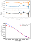 |
Fig. A.1. Top panel: stellar light curve and time variable flux-correction factors. Bottom panel: light curve of Mrk 1018 in the bright and transition phase, before and after flux corrections are applied following the method in Appendix A. |
Appendix B: Ratio spectrum calculation
The average model spectrum in the bright/faint state is defined as
 (B.1)
(B.1)
where Fstate,i(E) is the evaluated model spectrum at the best-fit parameters from the M3 model fits (Sect. 3.1 and Table 2) for either bright or faint state. The error bar, σstate(E), at each defined flux value here is the 90% confidence level calculated by evaluating the model on a subset of 500 samples selected randomly from the parameter-posterior distribution. The flux ratio at a given energy is defined by
 (B.2)
(B.2)
where the average in the ‘bright’ state is taken over XMM1, XMM2, and SUZ, and the ‘faint’ state is taken over XMM3, XMM4, and XMM5. The uncertainty in the ratio is given by
 (B.3)
(B.3)
The UVM2 bright to faint state flux density ratio (RUVM2) is calculated using the data point from the XMM-Newton observations. The energy band for UVM2 is EUVM2=(5.52±1.52)×10−3 keV.
The ratios R(E) and RUVM2 are plotted in Fig. 6.
Appendix C: UV seed and X-ray variability
Here, we describe how the extreme variability in an accretion disk is transferred to a static lamp-post corona. This exercise helps us understand the relation between the flux drop factors in the UV band vs. that of the X-ray band. The hot-corona X-ray emission is the up-scattered emission from the accretion disk. The variable disk emission at a given radius can be modeled by the emission from a thermal accretion disk (Shakura & Sunyaev 1973), given by
 (C.1)
(C.1)
In the above expression,  , where all parameters are constant and the variabilily is introduced by the modified sigmoid function (MRS), flong(t) (Sect. 3.6). Here the efficiency factor η is 0.057 as adopted by Kubota & Done (2018), λEdd is 0.02, and MBH = 107.9 M⊙. The parameters of the MRS functions are R = 24.5, t0 = 2200 days, and tsc = 365 days (Sect. 3.6).
Here, we considered the dominant UV emitting inner disk region to be between rtrunc = 30 Rg and ro = 70 Rg. The variable accretion rate Ṁ(t) wavefront begins at an instability location ro and travels inward (r<ro) at a finite speed v down to the truncation radius rtrunc. While the disturbance propagates through each annulus it also transmits seed photon ‘signals’ to the corona, which has a finite radius of a and is located at a height hX = 30 Rg above the disk-plane of the axis of symmetry. The seed photon signal received by the corona is subject to delays due to (a) the finite speed of v (<cs, the speed of sound) of wave propagation in the disk, and (b) the delay from the light-travel time for the distance  . The total delayed time of the wavefront is thus given by
 (C.2)
(C.2)
The radiation intercepted by a hot spherical lamp-post corona from a disk annulus at radius r is given by
![Mathematical equation: $$ dL_{\mathrm {cor, inc}}(t,r) = 2\pi r F_{\mathrm {disk}}(r, t_{{\mathrm {delay}},t,r}) \frac {\pi a^2 h}{[h^2_{\mathrm {X}} + r^2]^{3/2}} dr. $$](/articles/aa/full_html/2025/07/aa54707-25/aa54707-25-eq131.gif) (C.3)
(C.3)
The above expression is integrated in the range rtrunc≤r≤ro. The total variable emission incident on the corona is thus given by  . We simulated the light curves signifying the emission intercepted by the corona for two different values of corona size, a = 2 Rg and a = 5 Rg.
The variability light curves of the intercepted seed photon (Linc,cor) and the total disk emission (LDisk) between rtrunc and ro (Fig. C.1) show that for two given corona sizes that are constant in time, the net amount of intercepted seed photons varies significantly, with no difference in the variability factor for any light curves. There is also negligible difference in the variability profiles since the net delays are not enough to smooth the light curves on timescales of tsc≃1 year. This indicates that we require a increased covering fraction of the hot X-ray emitter with respect to the UV emitter (i.e., variable hX, corona size a) in the faint state to obtain different values of long-term flux drop in the UV and the X-ray waveband.
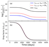 |
Fig. C.1. (a) Top panel: Incident seed luminosity (log Linc,cor) on a corona of radius 2Rg (blue), radius 5Rg(red) and the accretion disk luminosity (Ldisk) (b) Bottom panel: Same light curves but normalized using the minimum luminosity value. The drop factors are equal. |
As a caveat, we note that the disk-corona model assumed here has a simple geometry. However, the phenomena reported above would be largely geometry independent. This is because the results depend on the physical extent of the corona with respect to the accretion disk, and our model effectively captures this aspect. Furthermore, we do not assume an inner ADAF despite the fact that the inner flow structure changes across accretion rates.
Appendix D: Energy budget during different phases of Mrk 1018's evolution
We have fit a modified reverse sigmoid function (Sect. 3.6) to the X-ray flux data post 2005. The best-fit light curve has captured the long term flux variability trend including the major flux drop post 2013. We then applied the X-ray bolometric corrections from Duras et al. (2020) to the long-term X-ray light curve LX−ray(t)) to obtain the long-term bolometric luminosity light curve, LBol(t). In the bright state, the excess luminosity generated compared to the faint state ΔLBol(t) =LBol(t)−LBol,faint. Thus, the excess energy emitted in the bright state compared to the faint state is ΔEbright=∫ΔLBol(t)dt. Integrating from 2005 to 2015, we obtain ΔEbright,2005−2015 = 2×1053 ergs. Assuming that the bright state had started in 1986 and ended in 2015 (Lu et al. 2025), i.e. continued for 30 years, and that the source has maintained the same average bright state flux in this period, the total power generated in the 30 year bright state phase is ΔEbright−phase≃3ΔEbright,2005−2015 = 6×1053 ergs. We can convert this estimate to the equivalent amount of mass accreted using ΔMbright−phase=ΔEbright−phase/ηc2, where accretion efficiency η is taken to be 0.057 (Kubota & Done 2018). We obtain ΔMbright−phase ≃6M⊙.
We also estimated roughly the energy emitted in the 2020 outburst (Brogan et al. 2023; Lu et al. 2025). The outburst extends for a comparatively short time, 1 year. We assumed that the outburst had the same peak luminosity as that of the pre-2010 bright state. Thus, it should have a total energy output of Eoutburst,2020∼2.5×1052 ergs (ΔMoutburst = 0.24M⊙). This estimate is approximately 25 times less than ΔEbright−phase, the energy emitted in the 30-year long ‘flare’ in the bright phase.
All Tables
Best parameter estimates obtained from BXA fits to the XMM-Newton and Suzaku datasets.
Average flux of the UVM2 (5.32 eV) band, X-ray spectral components, and bolometric luminosity with their respective flux drop.
All Figures
|
Fig. 1. XMM-Newton EPIC-pn pattern-0 data−model residuals from the X-ray spectral fitting using the models described in Sect. 3.1. Left: Bright state observation XMM2 (2008). Right: Faint state observation XMM4 (2019). Significant improvement in the residuals can be seen in both of the multicomponent models, M2 and M3, compared to the single power-law model, M1. |
| In the text | |
|
Fig. 2. Unfolded best-fitting models for the XMM-Newton EPIC-pn pattern 0 and Suzaku XIS-0 data. The spectral model is the best-fitting, physically motivated model M3 (Sect. 3.1). Solid curves: model evaluated at best fit value; dotted curves: model evaluated at the upper limit; blue markers: unfolded data; red curve: soft X-ray excess modeled by compTT; magenta curve: hot-corona power law; green curve: uxclumpy torus reflection model; black curve: the total unfolded X-ray spectrum. Panels (a), (b), and (c) show bright-state spectra; panels (d), (e), and (f) are for the faint state. These plots illustrate how all X-ray spectral components drop significantly in flux. The strongest drop is for the soft excess, which ultimately disappears in 2021. |
| In the text | |
|
Fig. 3. Overview of UV and X-ray spectral components. (a) De-reddened and host-galaxy subtracted UVM2 flux from combined XMM-Newton OM and Swift UVOT data. (b) Integrated total hard X-ray flux. (c) Photon index (Γ) of the hot corona power law (zpowerlwin M3; Sect. 3.1). (d) Integrated flux of the soft excess flux component (0.3–2.0 keV). (e) Integrated flux of the reflection component (2.0–10.0 keV). (f) Integrated Fe Kα emission line flux. Black-circular points: XMM-Newton; brown triangular points: Swift; blue diamond point Suzaku; and green square points: Chandra. The red vertical lines mark the beginning and end of the 2020 outburst in the optical band (Brogan et al. 2023). |
| In the text | |
|
Fig. 4. Broadband SED fits using the agnsed model. (a) Absorbed total broadband model. The circular markers indicate XMM-Newton EPIC-pn+OM datasets for the XMM3, and XMM5 observations and XMM-Newton EPIC-pn + OM + Swift-UVOT datasets for XMM2. The solid lines of corresponding color represents the best-fit total models. The XMM1 and XMM4 data points are not plotted for clarity. For XMM3 and XMM5 the OM photometric points almost overlap with each other since they have almost equal fluxes. (b) Corresponding unabsorbed agnsed models. They indicate the significant changes occurring in the intrinsic spectrum, within both the bright and faint flux states. The dashed lines indicate energies used to calculate the optical-X-ray spectral index αOX. |
| In the text | |
|
Fig. 5. (a) Light-curve data of UVM2 and best-fit MRS function normalized by the faint state flux. (b) Corresponding UVM2 residual. (c) Data of the 2–10 keV X-ray light curve and best-fit normalized by the faint state flux. (d) Corresponding X-ray residual. The circular, diamond, triangular, and the square markers represent XMM-Newton, Suzaku, Swift, and Chandra datasets, respectively. The red line indicates the best-fit MRS model. |
| In the text | |
|
Fig. 6. Energy resolved bright and faint state flux ratio. The solid black line is the ratio of the average X-ray spectra (R(E)) in the bright and the faint phase and the dashed lines demarcate the upper and lower error. The plot is based on the M3 model compTT + zpowerlw + uxclumpy-reflect calculated for the high-count XMM-Newton and Suzaku spectra. The UVM2 flux ratio (diamond marker) is derived from XMM-Newton OM observations. |
| In the text | |
|
Fig. 7. Evolution of the photon index (Γ) of the intrinsic hot corona power law with respect to the Eddington ratio (λedd=Lbol/Ledd). The different colors represent different missions: green, Chandra; red, Chandra observation from 2010 evaluated from readout streak; blue, XMM-Newton; orange, Suzaku; brown solid line, linear regression best-fit in the softer-when-fainter state; brown dashed line, the uncertainty range of the linear fit. The soft-when-fainter trend is evident for log λEdd<−1.7. |
| In the text | |
|
Fig. 8. Illustration of one possible geometrical change in AGN accretion structures due to the major CLAGN transition occurring after 2013. Length scales as illustrated here are approximate only. (a) Bright state configuration: warm corona present in the inner accretion structure along with the hot-accretion flow or corona or less dominant ADAF. (b) Faint state configuration after ∼2021: warm corona disappears (Sect. 4.2) and the inner accretion flow becomes dominated by a hot ADAF (Sect. 4.3), emitting X-rays and UV seed. The thin disk also decreases its energy contribution and physical size. Finally, the broad line region (BLR) + torus system extends from sub-parsec scale to 10 s of parsecs, which results in significant smoothing of the Fe Kα line response (Sect. 4.6.1 and Fig. 9). |
| In the text | |
|
Fig. 9. Response of an extended parsec-scale structure with inner radius of Rin = 0.01 pc line response and outer radius Rout = 10 pc. The dashed lines correspond to the upper and lower errors of Rout. Inset: Reduced-χ2 from the Fe Kα light-curve fit best estimate of the external radius. The blue marker and red dashed line represent the best-fitting value, and the error bar corresponds to Δχ2 = 5. |
| In the text | |
|
Fig. 10. Spectral fits to the Fe Kα line from C2 (2016), XMM3 (2018), XMM4 (2019), and XMM5 (2021; datasets are grouped for clarity). The dashed lines indicate the profile corresponding to the upper and lower error bars of σFeKα. The spectra have been normalized using the underlying continuum model. The relative strength or intensity of the Fe Kα line with respect to the continuum is significantly highest for C2 and XMM5 and lowest for XMM3. |
| In the text | |
|
Fig. 11. Time evolution of Fe Kα equivalent width, which exhibits a mild increase with time. Black circular markers: XMM-Newton; blue diamond marker: Suzaku; unfilled green square marker: Chandra from 2016 (C2); green square markers: all other Chandra spectra. |
| In the text | |
|
Fig. A.1. Top panel: stellar light curve and time variable flux-correction factors. Bottom panel: light curve of Mrk 1018 in the bright and transition phase, before and after flux corrections are applied following the method in Appendix A. |
| In the text | |
|
Fig. C.1. (a) Top panel: Incident seed luminosity (log Linc,cor) on a corona of radius 2Rg (blue), radius 5Rg(red) and the accretion disk luminosity (Ldisk) (b) Bottom panel: Same light curves but normalized using the minimum luminosity value. The drop factors are equal. |
| In the text | |
Current usage metrics show cumulative count of Article Views (full-text article views including HTML views, PDF and ePub downloads, according to the available data) and Abstracts Views on Vision4Press platform.
Data correspond to usage on the plateform after 2015. The current usage metrics is available 48-96 hours after online publication and is updated daily on week days.
Initial download of the metrics may take a while.