| Issue |
A&A
Volume 699, July 2025
|
|
|---|---|---|
| Article Number | A258 | |
| Number of page(s) | 19 | |
| Section | The Sun and the Heliosphere | |
| DOI | https://doi.org/10.1051/0004-6361/202554559 | |
| Published online | 17 July 2025 | |
The effects of expansion and turbulence on the interplanetary evolution of a magnetic cloud
1
Dipartimento di Fisica e Astronomia, Università degli Studi di Firenze, Via G. Sansone 1, 50019 Sesto Fiorentino, Italy
2
Istituto di Astrofisica e Planetologia Spaziali, Istituto Nazionale di Astrofisica, Via del Fosso del Cavaliere 100, 00133 Roma, Italy
⋆ Corresponding author: mattia.sangalli@unifi.it
Received:
16
March
2025
Accepted:
13
May
2025
Coronal mass ejections represent the most extreme solar products, and show complex and dynamic structures when detected in situ. They are often preceded by a shock and carry a magnetic cloud organised as a flux rope, surrounded and permeated by turbulent fluctuations, and whose radial size expands during propagation. We investigate the internal dynamics of the 2D section of a cylindrical flux rope propagating at a constant velocity in the spherically expanding solar wind. To do this, we employed the expanding box model, which allows for high spatial resolution. We used a simplified setting with a uniform and non-magnetised solar wind, on which we superpose turbulent fluctuations. We find that the spherically expanding geometry alone perturbs the flux rope equilibrium and produces a radial head-tail velocity profile and a radial size increase. The ratio between the expansion and Alfvén timescales, which are associated to propagation and internal crossing time respectively, controls the resistance to transverse stretching and the increase of the flux rope radial extent; the plasma beta controls the overall size of the structure. Turbulent fluctuations mainly affect the flux rope transverse structure and spread its axial field at distances comparable to its size; on the contrary, dynamics along the radial direction remains coherent and the increase in radial size is still consistently observed. We validate our results by comparison with statistical observations and dimensionless estimates, such as the expansion parameter and the radial size scaling exponent. Such a comparison suggests that the ratio between internal and propagation timescales might help in better classifying different kinds of radial expansion for flux ropes.
Key words: magnetohydrodynamics (MHD) / turbulence / methods: numerical / Sun: coronal mass ejections (CMEs)
© The Authors 2025
 Open Access article, published by EDP Sciences, under the terms of the Creative Commons Attribution License (https://creativecommons.org/licenses/by/4.0), which permits unrestricted use, distribution, and reproduction in any medium, provided the original work is properly cited.
This article is published in open access under the Subscribe to Open model. Subscribe to A&A to support open access publication.
1. Introduction
Coronal mass ejections (CMEs) are large-scale eruptive events that take place in the Sun's outer atmosphere and involve the release of plasma and magnetic fields (Webb & Howard 2012). The ejected material propagates in the solar wind, becoming an interplanetary CME (ICME). ICMEs often display a complex multi-part structure that possibly includes a leading shock wave (see e.g. Gosling et al. 1975; Sheeley et al. 1985), a compressed and turbulent sheath region (Kilpua et al. 2017), and an enhanced magnetic field (magnetic cloud or ejecta) (see e.g. Klein & Burlaga 1982; Burlaga 1988). The latter can be thought of as a magnetic flux rope, with both extremities connected to the Sun (see e.g. Burlaga 1988; Bothmer & Schwenn 1998). Coronal mass ejections drive the most intense geomagnetic storms (Gosling et al. 1991; Webb et al. 2000; Huttunen & Koskinen 2004; Zhang et al. 2007; Richardson & Cane 2012) and their sheath regions play a key role in further enhancing the geoeffectivity (Huttunen & Koskinen 2004; Kilpua et al. 2017).
Turbulence is not only found in the background solar wind (Goldstein et al. 1995; Bruno & Carbone 2013), but also in ICMEs, both in magnetic clouds (e.g. Ruzmaikin et al. 1997; Leamon et al. 1998; Manoharan et al. 2000; Sorriso-Valvo et al. 2021) and in sheath regions (e.g. Kennel et al. 1982; Kataoka et al. 2005; Kilpua et al. 2017). Stronger turbulence is usually found in sheath regions (Good et al. 2020; Kilpua et al. 2020; Sorriso-Valvo et al. 2021; Márquez Rodríguez et al. 2023), but magnetic clouds also show a consistent fraction of energy in the fluctuations (Leamon et al. 1998), with a wide range of spectral indices (Borovsky et al. 2019) and regardless of the subtraction of the large-scale flux rope field (Good et al. 2023). Recently Pezzi et al. (2024) performed 3D compressible magnetohydrodynamics (MHD) simulations of turbulence interacting with a large-scale magnetic flux rope that show that the flux rope inhibits the cascade of weak fluctuations but is overcome by sufficiently strong ones.
Moreover, multi-spacecraft analyses have shown that ICMEs have a fine-scale structure, with magnetic coherence lengths of both magnetic ejecta (Lugaz et al. 2018) and sheath regions (Ala-Lahti et al. 2020) being smaller than the ICME size: magnetic scale lengths estimated at 1 AU can be as small as 0.024 AU (ejecta) and 0.06 AU (sheath), whereas ICMEs have estimated sizes around 0.3 AU. A number of factors might explain the presence of this meso-scale structure, including their properties upon release in the coronal environment, their internal evolution, and the interaction with the surrounding medium during heliospheric propagation.
During their journey in the heliosphere, ICMEs increase their transverse and radial size, as is already apparent in remote sensing observations (see e.g. Patsourakos et al. 2010). While the expansion in the transverse direction can be explained as a consequence of the spherical flow of the ICME, its expansion in the radial direction is thought to originate from magnetic over-pressure with respect to the ambient solar wind (Démoulin & Dasso 2009). The increase in the radial size was first observed indirectly in magnetic clouds (Kumar & Rust 1996; Bothmer & Schwenn 1998) and more generally in ICMEs (Liu et al. 2005; Wang et al. 2005); it was then found as an almost linear head-tail proton velocity difference (Lepping et al. 2003, 2008; Jian et al. 2008). Statistical studies find the radial size, S, to increase with heliocentric distance, R, as a power law S(R)∝RαR, and give the scaling index, αR, as a ‘global’ estimate of radial expansion, whereas the velocity profile gives a local estimate of the physical dilation that the plasma is experiencing. Assuming the internal Alfvén time to be much shorter than the travel time, along with an assumptions of a local cylindrical geometry, Démoulin et al. (2008) linked the local velocity profile to the power-law scaling exponent by means of a non-dimensional expansion parameter. Such locally estimated scaling exponents for unperturbed magnetic clouds at 1 AU are around unity (0.81±0.19 in Démoulin 2010, 0.91±0.23 in Gulisano et al. 2010). However, further studies using aligned radial measurements suggest quite weak correlations between global and local expansion estimates (Lugaz et al. 2020).
One of the main tools for investigating the evolution of ICMEs is offered by global numerical simulations. Numerical models such as WSA-ENLIL+Cone (Odstrcil et al. 2004) and EUHFORIA (Pomoell & Poedts 2018) can reproduce complex heliospheric configurations including multiple CMEs and structured solar wind (see also Manchester et al. (2017) and references therein). Despite capturing many important features of the 2.5D and 3D heliospheric and interplanetary evolution of CMEs, such as the aforementioned transverse and radial expansion, global simulations usually lack the numerical resolution to resolve the ICME fine structure and the physical processes occurring at those scales, such as turbulence and magnetic reconnection.
Here, we present a novel approach to simulate the interplanetary evolution of a CME with an embedded magnetic cloud. We employ a semi-Lagrangian numerical model, the expanding box model (EBM), first introduced by Grappin et al. (1993), which allows us to decouple the internal MHD dynamics from the large-scale motion. With the resulting high resolution, we investigate the impact of meso-scale internal processes on the evolution of the magnetic cloud; we focus on the interaction of the magnetic configuration with the anisotropic expansion and on the effect of superposing turbulent fluctuations on such a system. Using EBM introduces an additional parameter to the usual MHD equations, the expansion rate, which controls the pace of spherical expansion and plays a key role in our study.
The structure of the paper is the following. In Sect. 2 we describe the EBM, the numerical setup, the magnetised equilibrium configuration used to describe the 2D section of a flux rope, and the main parameters used for the different simulations, focusing on the definition and meaning of the non-dimensional expansion rate, ɛ0. Sections 3 and 4 present the results of our simulations of an expanding magnetic cloud, without and with turbulent fluctuations, respectively: the contributions of spherical expansion, internal dynamical balance, and turbulence are qualitatively and quantitatively examined. In Sect. 5, we compare our findings to previous theoretical and observational studies and examine our results in a broader context. The final section summarises our main findings and discusses the limitations and perspectives of this work.
2. Equations, numerical methods, initial conditions, and parameters
2.1. Ideal MHD equations in EBM
In what follows we employ the expanding box model (EBM, Grappin et al. 1993; Grappin & Velli 1996; Rappazzo et al. 2005; Dong et al. 2014) to follow the evolution of a parcel of plasma in the spherically expanding solar wind. Below we give a heuristic description of the EBM, focusing on its physical interpretation. A more rigorous derivation can be found in the above works.
We assume a mean wind velocity  , which transports the parcel radially outwards from the Sun. By doing so, the large-scale radial motion of the plasma is decoupled from the small-scale internal dynamics, which is numerically solved inside the simulation box. The heliocentric position of the parcel of plasma is given by
where R is the radial (heliocentric) coordinate, starting at R(t = 0) = R0, and U0 is the constant radial velocity. Since we are considering a spherically expanding plasma, the box expands as a unit element of spherical volume: while moving outwards, the transverse size of the domain increases linearly with R because of the assumed radial flow, while the radial size remains constant. The expansion rate is given by U0/R0, and is the inverse of the characteristic expansion time, texp=R0/U0, which is also the transport (propagation) time. In the following we use the heliospheric distance normalised to its initial value:
The use of EBM implies a couple of relevant modifications to the usual MHD equations, which are now written in a reference frame that is comoving with the box. In this frame, the large scale flow is absent and we are left with the velocity fluctuations with respect to the mean flow, u=U−U0. Now all variables depend only from the local coordinates,  where ∥ and ⊥1, ⊥2 refer to the radial direction and to the two transverse directions. Spherical expansion implies that the transverse dimensions change with time (distance), while the radial one is constant,

The geometrical stretching is thus incorporated by multiplying the gradients in the usual MHD equations by anisotropic factors
In what follows, we shall concisely write ‘⊥’ without specifying ‘for ⊥=⊥1,⊥2’.
This leads to the non-dimensional ideal MHD equations in the EBM:
where thermodynamic variables are related through the equation of state P=ρT and all the variables are to be intended as functions of the comoving and expanding Cartesian coordinates (x′,y′,z′); moreover, ℐ is the 3×3 identity matrix and  is the projector on the transversal directions

The frictional forces (i.e. the additional linear terms in the right hand side (r.h.s.) of Eqs. (5)) make all the fields decay with different scaling laws: for the number density

for the magnetic field components

and for the local velocity field components,

Finally the temperature decreases as

where γ is the adiabatic index chosen as equal to 5/3.
The non-dimensional form is obtained defining the characteristic length (L0), mass density (ρ0), and magnetic field (B0). The other quantities are all expressed in Alfvén units: velocities are measured in Alfvén speed,  ; time in Alfvén time, t0=L0/u0; temperature in Alfvén units T0=mp(u0)2/2kB. Units are chosen relative to the initial configuration of the flux rope, so that L0≡LFR and B0≡BFR are the width and the axial field of the flux rope, while ρ0≡ρbg is the uniform ambient solar wind density (also equal to the flux rope density – see next section for details on the initial configuration).
Since the expansion rate U0/R0 is an additional dimensional parameter with respect to the usual MHD equations, defined through U0 and R0, its non-dimensional counterpart is related to the velocity and length units (i.e. also to the magnetic field and density ones). The non-dimensional expansion rate ɛ0 is then the ratio between the unit time t0 (in our case, the characteristic Alfvén time1) and the expansion time texp:
and its value controls how fast the expansion is with respect to the flux rope's crossing time.
2.2. Choice of geometry and numerical methods
Throughout this work, we consider the coordinate x∥=x′ as the locally radial coordinate and therefore x⊥1=y′ and x⊥2=z′ as the locally transverse coordinates. This implies that the projector on the transverse (non-radial) directions is  and ∇′=(∂/∂x,(1/a)∂/∂y,(1/a)∂/∂z). We then consider a magnetic flux rope whose curvature radius is much larger than its initial radial size: this assumption of local cylindrical symmetry allows us to neglect the dynamics along the flux rope axis. We consider z′ to be directed along the axis, which implies ∂/∂z′≡0, and the dynamics takes place in the plane (x′,y′) normal to the axis. We also assume a 2.5D geometry, such that u and B have all three vector components. The 2D simulation domain is thus made of a radial (x) and a transversal (y) direction. A schematic representation of the configuration is shown in Fig. 1. We are thus working in a comoving and expanding reference frame, which contains the cross section of a magnetic cloud and is moving away from the Sun with a constant radial velocity; this means that we assume the plasma flow to be everywhere spherical (absence of non-radial motions) and uniform (no acceleration or deceleration of the large-scale flow); moreover, we assume the background solar wind to be non-magnetised. In doing so, we implicitly impose that the internal kinematics of the flux rope follows the spherical expansion in absence of (internal or external) forces.
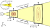 |
Fig. 1. Geometry and coordinate system for the expanding box model. We define x as the spatial coordinate along the mean flow (local radial coordinate), z as the local direction of the flux rope axis (along which the fields are assumed to be invariant), and y completes the right-handed system. The flux rope has an initial circular section. The position of the box is R(t), which increases with time as the flux rope propagates away from the Sun. |
We assume all the fields to be periodic in the local coordinates (x′,y′) and constant in the axial (out-of-plane) coordinate z′. The numerical code integrates the viscous and resistive EBM equations on a domain Lx×Ly, with a fixed grid Nx×Ny, and is based on a pseudo-spectral 2.5D code already employed for example in Papini et al. (2021). Fourier transforms are used to compute spatial derivatives via the FFTW library (Frigo & Johnson 2005), and a third order Runge-Kutta method is used for time advancement (Wray 1990). The full equations are described in Appendix B, and employ the out-of-plane component of the magnetic vector potential Az (in order to ensure ∇·B = 0) and rescaled versions of the physical variables (in order to use the equation for magnetic potential also with EBM, as devised by Rappazzo et al. 2005).
In addition to the physical variables, a passive scalar s is evolved, which follows an advection equation

The passive scalar is used as a tracer of the flux rope material and is initialised in two regions (see next section).
2.3. Initial equilibrium and flux rope identification
We initialise the simulations by imposing a 2.5D profile for the flux rope equilibrium, and use the local cylindrical coordinates (r′,θ′,z′) to better exploit our assumption of cylindrical symmetry; the (r′-θ′) plane corresponds to the (x′,y′) plane normal to the flux rope axis. No ambient magnetic field is present.
The configuration is static, stationary and axially symmetric around the flux rope axis. This means that  and P=P(r′). With such assumptions the condition for a stationary and static equilibrium reads (from now on, the primes are dropped for better readability):
The equilibrium results from a balance of three forces: the magnetic pressure gradient (Bθ and Bz) that pushes away from the axis; the magnetic tension (Bθ) and the kinetic pressure gradient (P) that pull towards the axis (the flux rope is colder than the environment). We assume uniform density throughout the domain, equal to the background ambient solar wind, ρ=ρbg; we choose a profile for both Bθ(r) and Bz(r), thus leaving P(r) to be analytically determined so as to account for the ultimate stability of the configuration. The pressure profile is thus computed as
where P(r = 0) is chosen so that P∞=ρbgTbg.
The profiles of the in-plane poloidal magnetic field (Bθ), the out-of-plane axial magnetic field (Bz), and pressure P (which are described in Appendix A) are shown as a function of the local radial coordinate r in Fig. 2 with blue, violet and orange lines, respectively. The profile of the passive scalar s is also shown as a grey line. The magnetic field has an axial component which is zero at infinity and rises to a peak Bz,0≡BFR (1 in code units) on the axis. The in-plane component vanishes at infinity and on the axis, with a peak Bθ,0=BFR/2 (0.5 in code units) at r=Δ=LFR/4 (0.25 in code units).
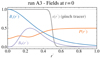 |
Fig. 2. Initial configuration of the main plasma parameters for the reference run A3. The solid lines show the axial out-of-plane magnetic field, Bz (blue), the poloidal in-plane magnetic field, Bθ (violet), the kinetic pressure, P (orange), and the passive scalar, s, as pinch tracer (grey), respectively, all as a function of the local radial coordinate, r′. |
We initialise two passive scalars in two overlapping regions for later use in identifying the flux rope material, especially in turbulent simulations. The ‘pinch tracer’, spinch, is initially limited to the region bounded by the in-plane (twisted) magnetic field. As can be seen in the figure, the pinch tracer has a half-width of LFR/2 (0.5 in code units), but both Bθ and Bz extend a bit further out because of their chosen functional form. For this reason we also use also an ‘axial tracer’, saxial, which is initialised to cover also the out-of-plane flux rope magnetic field, to keep track of its transport that is not constrained by the pinch provided by the in-plane magnetic field. The primary use of the pinch tracer is to return an estimate of the radial and transversal sizes of the flux rope from the simulations. We use an integrated measure of the flux rope size, computed as the standard deviation of each coordinate using the pinch tracer s as weight:
where
and similarly for y.
Once the simulation starts, expansion causes an anisotropic stretching of the domain and the decrease of field components and temperature, and thus perturbs this initial equilibrium. The anisotropic scaling of kinetic and magnetic pressure terms (coming from Equations (7), (8) and (10)) already suggests a natural decrease of the plasma β, which would result in an over-expansion in all directions, since the kinetic pressure decays more rapidly with heliocentric distance than the magnetic pressure does, asymptotically:
2.4. Turbulent fluctuations and spectral quantities
To study the effect of turbulence on the evolution of the flux rope in the expanding geometry, we perturb the initial equilibrium with pseudo-Alfvénic fluctuations with zero divergence and zero mean cross helicity, δu and δB, which naturally develop into MHD turbulence (as in Papini et al. 2019). We arbitrarily fix the amplitudes of the 2D Fourier coefficients  and
and  to decrease as k−1/2, with
  , resulting in an omnidirectional 1D flat (horizontal) power spectral density. We further define kFR = 2π/LFR and the minimum wave-number k0 = 2π/Lx, the latter depending on the domain size. Fluctuations are completely determined by the choice of two further parameters: the interval of excited (‘turbulent’) scales, kturb∈[k1, k2], and the root mean square (RMS) amplitude of fluctuations,
  . Their value determines an additional non-dimensional parameter,
where tNL=(k1δu)−1 is the non-linear time computed at the largest scale of turbulent fluctuations and where the Alfvén time is the same as our unit time  . Since we fixed Bθ,0/Bz,0 = 1/2 in our runs, the value of χ controls how fast the turbulent dynamics is compared to the flux rope's crossing time. The ratio χ/ɛ0=texp/tNL defines the ‘age’ of turbulence, that is, how fast turbulence evolves with respect to the expansion and propagation time; its inverse then defines the ‘turbulent expansion rate’:
As a rule fluctuations are excited in the whole domain, including the flux rope, with one exception (see next section).
In analysing turbulent simulations we compute the power spectral density for the velocity and magnetic fluctuations. The power spectral density of a vector field f is the omnidirectional 1D spectrum, obtained by summing the square of the 2D Fourier coefficients,  , which have wave-numbers that fall in a shell of thickness [ki, ki+1),
The grid of shells of the omnidirectional spectrum is fixed at all times and equal to the wave-numbers of the non expanding direction, ![$ k_i\in [k_x^{\min },k_x^{\max }] $](/articles/aa/full_html/2025/07/aa54559-25/aa54559-25-eq37.gif) ; since the wave-numbers in the transverse direction decrease as 1/a, we account for the anisotropic stretching by computing
; since the wave-numbers in the transverse direction decrease as 1/a, we account for the anisotropic stretching by computing  . With this choice the large wave-numbers in the transverse direction always contribute to the omnidirectional spectrum, but the large scales
  (including part of the flux rope) are left out.
As already pointed out by Grappin & Velli (1996) and Dong et al. (2014), the expanding geometry weakens the spatial gradients and damps fluctuations, and thus slows down the non-linear dynamics of turbulence. Recently Pezzi et al. (2024) perturbed a cylindrically symmetric flux rope by exciting 3D turbulence in the whole domain (homogeneous MHD, no spherical expansion); their results show that for weak fluctuations the large-scale coherent magnetic field inhibits the turbulent cascade towards small scales, whereas for strong fluctuations the cascade dominates and the flux rope can get strongly perturbed. Although in this study we are limited to 2D turbulence interacting with a 2.5D flux rope, we also aim to understand how much exciting fluctuations inside the flux rope counts in perturbing the equilibrium.
2.5. Main parameters and simulations dataset
We summarise now the main control parameters and comment briefly the simulations dataset used throughout the paper. We recall that the initial equilibrium of the flux rope is the same in all runs and determines the code units, Bz,0 = 2Bθ,0=BFR = 1, LFR = 1, ρbg = 1.
2.5.1. Expansion rate, plasma beta, and fluctuations
We carry out a series of simulations with a flux rope embedded in a uniform background (isolated flux rope, runs labelled with A, B, C, and D). These runs are completely determined by two parameters: the plasma β, common to standard MHD, here evaluated as the ratio between the external pressure and the flux rope's magnetic field
and the non-dimensional expansion rate, ɛ0 (Eq. (11)), which controls how fast the spherical expansion is compared to the flux rope crossing time. We focus on run A3 to thoroughly describe the evolution and internal dynamics in Sects. 3.1 and 3.2.
The second series of simulations explores the impact of turbulence on the flux rope dynamics: the parameters are the same as in run A3, and fluctuations are added (runs labelled with Y and Z); as a rule we excite fluctuations in the whole domain, thus also inside the flux rope (runs Y3, Y3h, Y3k), but since observations generally indicate that fluctuations are smaller inside the flux rope that outside of it (Regnault et al. 2020; Sorriso-Valvo et al. 2021), we also consider one case in which the amplitude of fluctuations is reduced by a factor 5 when entering the flux rope (run Z3). The addition of fluctuations introduces the non-dimensional parameter χ=tA/tNL, which controls how fast the non-linear turbulent dynamics is compared to the flux rope crossing time; the turbulent expansion rate ɛT=tNL/texp then controls how fast the expansion is compared to the turbulence timescale. We focus on run Y3 to thoroughly describe the effects of turbulence in Sect. 4.
We do not attempt a complete scan of the parameter space, since it should also involve variation of the initial equilibrium (e.g. the degree of twist of the flux rope Bθ,0/Bz,0) and of the turbulent spectrum (e.g. the range of excited wave vectors and its energy distribution); we prefer to select values that are reasonable in terms of the physical system of interest. For the isolated runs, we choose values of ɛ0∈[0.2,3.2] (runs A2-A6), with more than an order of magnitude of separation. Then we fix ɛ0 = 0.4 and vary instead β0 by varying Tbg, in a range β0∈[0.6,4.0] (runs B3, A3, C3 and D3), with values below and above unity.
The simulations labelled with Y and Z have random fluctuations initially superposed on the flux rope: simulations Y3, Y3h and Y3k all have the same parameters as A3 and δB/BFR = 0.5: run Y3h is the same as Y3 but with no expansion (regular MHD); run Y3k is the same as Y3 but with fluctuations at smaller scales; run Z3 is the same as Y3 but with smaller fluctuations inside the flux rope. For the turbulent runs, our choices of δB/Bθ,0∼1 (strong turbulence) and kturb/kFR≳1 (fluctuations on smaller scales than the flux rope) imply χ≳3, that is, a quickly developing turbulence with respect to the flux rope crossing time. The expanding runs Y3, Y3k and Z3 all have ɛ0 = 0.4, so ɛT≲0.13 (fast turbulence compared to expansion); a value ɛT≲1 is required to have a dynamically relevant turbulence during the propagation, otherwise the non-linear cascade would take too much time and the turbulence would be ‘frozen’ during the propagation. Run Y3k has an ɛT four times smaller than run Y3, that is, a quicker (shorter-lived) turbulence.
For runs labelled with A, B, C, and D, we use open boundaries in the x direction (similarly to Rappazzo et al. 2005), whose details will be given in a separate work. The results were tested to be the same with open and periodic boundaries, but using open boundaries allows us to avoid spurious reflections without needing a wider domain and more grid points.
2.5.2. Interpretation of the non-dimensional expansion rate and limitations
Since the non-dimensional expansion rate ɛ0 is given by four different quantities (recall Eq. (11)), a value of 1 corresponds equally to a flux rope starting at R0 = 5LFR with a speed  , or to a flux rope that is initially closer to the Sun and moves slower of the same factor. However, our assumption of constant speed is not well justified close to the Sun, because of the initial driving phase to which CMEs are subject; a CME can be thought of as isolated and interacting with just the solar wind only after a distance of about 20 to 30 R⊙ (see e.g. St. Cyr et al. 2000; Subramanian & Vourlidas 2007; Sachdeva et al. 2015). We thus fix the starting heliocentric distance to be 30 R⊙ for all the simulations.
Our parameter ɛ0 then reflects three free parameters in L0=LFR, U0 and  , which all contribute to set the ratio between expansion and Alfvén timescales. However, CMEs have a quite diverse range of sizes, velocities, and magnetic field intensities, and this can result in a broad range of values for ɛ0 because of a difference in one quantity, or equal values of ɛ0 for very different CMEs. To ease the physical interpretation of ɛ0, one can think of fixing the background density and magnetic cloud peak field, thus fixing
  , and also the initial flux rope size: varying ɛ0 then corresponds to varying the CME propagation velocity. The relation of ɛ0 to actual flux rope parameters is further discussed in Sect. 5, and run AR is also described there. It should be kept in mind that the meaning of ɛ0 is the ratio between the internal Alfvén and the large-scale propagation (expansion) timescales.
Because of the functional form of our initial equilibrium configuration, which requires a dip in the temperature profile in order to confine the magnetic flux rope, we cannot choose a background temperature too low, since the resulting value inside the flux rope would become negative. This possibly limits us to a narrower range of β0 values than what is generally observed (again, see discussion in Sect. 5).
Independently of the other parameters, all simulations are run up to the same final distance, R = 7.4R0≃1 AU, that is: the smaller the expansion rate, the longer the time it takes to get to 1 AU (see t1AU in Table 1).
List of parameters for the simulations.
3. Results: Internal dynamics and spherical and radial expansion
3.1. Heliospheric evolution
The evolution of magnetic field (|B|), radial velocity (ux), transverse velocity (uy), and density (ρ) is shown in Fig. 3 for run A3. Time (or distance) runs from left to right in each row and is indicated in the top panels. We note that for a better visualisation, only a part of the transverse domain is shown and all quantities are rescaled by the average decay expected from conservation of linear invariants, Eqs. (7)–(9), as indicated next to the colour bars.
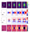 |
Fig. 3. Run A3. From top to bottom: evolution of magnetic field |B| (a), velocity ux (b) and uy (c), and density ρ (d). For |B| and ρ, the fields’ decay with heliocentric distance has been compensated for better visualisation. The in-plane magnetic field is represented in panels (a-c) as constant-Az black lines, whereas the outermost boundary of the pinch tracer is represented in panel (d) as a dashed white line. All the quantities are in code units. |
The in-plane magnetic field is also shown as constant-Az solid lines in Figs. 3a-c, whereas the outermost boundary of the pinch tracer is shown in Fig. 3d as a dashed line. The tracer follows pretty well the flux rope boundary as identified by the in-plane magnetic field and is redundant at this stage. However, it is necessary to identify the flux rope material in presence of turbulent fluctuations in Sect. 4. For consistency, we use the tracer throughout the paper to determine the flux rope extent along the x and y directions.
In the top panels one can see that during the radial propagation, the isotropic initial equilibrium configuration is stretched in the transverse direction due to the large-scale motion of the box, as expected from the spherical geometry; a closer view of panel (a) shows that the flux rope's radial size Sx increases with time, whereas its transverse size Sy seems to increase less than linearly with distance; the result is an anisotropic configuration. We recall that a passive plasma structure subject to spherical expansion would undergo a ‘kinematic expansion’, that is, its radial size would remain constant whereas its transversal size would increase linearly with heliocentric distance (recall Eq. (3)). The flux rope's radial expansion implies an aspect ratio smaller than the ‘kinematic’ one, at any given distance.
Deviations from the kinematic expansion can be roughly explained by considering the evolution of the total dynamical pressure. Since the magnetic field is present only inside the flux rope and recalling Eq. (16), it follows that
so that the internal over-pressure produces a (locally) outward force, which brings to the radial expansion.
Inspection of the top panels in Fig. 3 shows the out-of-plane Bz (colour-coded) and the in-plane Bθ (black iso-lines) magnetic field components to follow slightly different evolutions: along the radial direction the extent of both components is about the same, but in the transverse direction Bz extends more than Bθ. Also, the velocity components ux and uy in panels (b) and (c), respectively, and the density in panel (d), reveal a richer dynamics.
As soon as expansion is triggered, a pressure wave is launched and propagates anisotropically away from the flux rope. This wave compresses the surrounding plasma and causes a dramatic drop of density inside the flux rope; the temperature T – not shown – has a very similar evolution, with heating outside and cooling inside; this perturbation contributes to keep β<1 inside the flux rope. At the same time a radial velocity pushes the magnetic field away from the flux rope centre, while the transverse velocity pulls it towards the centre. The larger transverse extent of Bz compared to Bθ is the result of this pulling force and of the initial condition (Bz tail extending beyond the region where Bθ≠0), and is not due to magnetic diffusion (we come back to this point later).
3.2. Dynamical analysis
A more quantitative description of the internal dynamics and kinematics of the flux rope can be obtained by looking at Fig. 4, where the extent of the flux rope tracer is shown as a shaded pink along 1D cuts passing through the centre in the x and y directions (left and right panels, respectively), for different times, t = 0,0.5,4.0 (from top to bottom); only half of the 1D domain is shown because it is symmetric with respect to the flux rope centre. The theoretical flux rope extent as due to the kinematic stretching of the box is drawn with a dark pink vertical line. By comparing the two bottom panels, it is clear that along the radial direction the flux rope has expanded, contrary to the constant-size prediction by simple kinematic expansion, while in the transverse direction the flux rope has expanded less than kinematically.
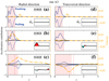 |
Fig. 4. Run A3. Evolution of the main dynamical terms (solid and dashed blue lines), their resultant (black line), and the velocity field (dash-dotted orange line, different scale), along both x (left panels) and y (right panels). The 1D cuts are taken at half domain (i.e. they intersect the flux rope axis). All the quantities are in code units and the dynamical terms are re-scaled relative to their maximum at t = 0. Only the right half of each 1D spatial domain is shown, since the dynamics is just inverted in the other half (axial symmetry). The computed (expected) pinch tracer size is shown as a filled light pink region (vertical line) for each snapshot. In the bottom right corner of each panel, an inset shows the resultant acceleration, |

To describe the dynamics of the flux rope, we also show in each panel the profile of the pushing and pulling acceleration terms. Pushing forces point away from the flux rope axis and are given by the magnetic pressure term (mainly the out-of-plane component). Their resulting acceleration is plotted with solid blue lines. Pulling forces point towards the flux rope axis and are given by magnetic tension (involving only Bθ) and the external (gas) pressure. Their resulting acceleration is plotted with dashed blue lines. The solid black line is the overall resultant acceleration, which includes all the terms in Eq. (5b); the dashed orange line is the profile of the velocity along the cut plotted on a different scale for better visualisation (ux and uy in the left and right panels, respectively); the inset shows again the total acceleration for better visualisation.
Along the radial direction (x), a magnetic over-pressure produces a pushing force at the edge of the flux rope, which in turn creates the outwards-directed velocity, that is, the radial expansion. Along the transversal direction (y), a pushing force is present as well but weaker, and the main dynamical term becomes magnetic tension, which produces a pulling force located inside the flux rope, which creates an inward directed velocity, that is, a local contraction.
The wavefront already visible in Fig. 3 can be more clearly identified, especially along x (centre and bottom rows); also, the prevailing of velocity-related dynamical terms such as −u·∇u at later times can be noted (bottom row); this information is especially visible in the inset of Fig. 4c. A hint to the different evolution of Bz and Bθ along y is visible in Fig. 4e, where positive and negative forces coexist around the boundary of the flux rope.
The forces involved in the flux rope equilibrium can be further analysed: the relative importance of the forces at early times can be estimated using the scaling laws for the evolution of gradients and fields in the EBM, namely Eq. (4) and Eqs. (7), (8), (10) (along with γ = 5/3). Substituting those scaling laws in Eq. (5b) and explicitly considering the x and y components, we obtain
![$$ \frac {\mathrm {d}u_x}{\mathrm {d} t} \propto -\frac {1}{\rho _{R_0}}\left [a^{-4/3}|\nabla _x P|_{R_0} +a^{-1}|\nabla _x P_\mathrm {m}|_{R_0} - a^{-2}|{\mathbb {T}}_x|_{R_0}\right ] $$](/articles/aa/full_html/2025/07/aa54559-25/aa54559-25-eq46.gif)
![$$ \frac {\mathrm {d}u_y}{\mathrm {d} t} \propto -\frac {1}{\rho _{R_0}} \left [a^{-7/3}|\nabla _y P|_{R_0} + a^{-3/2}|\nabla _y P_\mathrm {m}|_{R_0} - a^{-1}|{\mathbb {T}}_y|_{R_0}\right ], $$](/articles/aa/full_html/2025/07/aa54559-25/aa54559-25-eq47.gif)
where on the r.h.s. the three terms represent the predicted scaling laws of kinetic and magnetic pressure gradients (respectively P and Pm) and magnetic tension ( ). Since the magnetic field components B∥ and B⊥ follow different scaling laws, for brevity we used their geometrical mean to evaluate the overall magnetic pressure gradient scaling. Along x, the magnetic pressure gradient dominates, explaining the net pushing force that is responsible for the increase of the radial size. The magnetic tension has the fastest decrease, suggesting a later dynamics dominated by magnetic and gas pressures. On the contrary, along y the magnetic tension dominates, explaining the net pulling force responsible for the less-than-kinematic increase of the transverse size. In this direction the gas pressure strongly decreases, suggesting a purely magnetic kind of dynamics between magnetic pressure and tension.
To evaluate the relative importance of the forces also at later times for run A3, in Fig. 5 we plot the heliocentric evolution of the pushing and pulling terms (top panels), separately for the radial (left) and transverse direction (right). In the top panels the expected scaling laws from Eq. (22) are also shown with dotted lines, while the contribution of the magnetic tension is plotted with filled grey circles. At any distance we compute quantities inside the region traced by the pinch tracer in order to filter out the outwards propagating acceleration associated with the wave. The difference between the pushing and pulling peak values returns a good estimate of the net acceleration. However, the maximum and minimum are not always co-spatial, so both positive and negative acceleration regions can coexist. This further information is supplied in the bottom panels where the minimum and maximum of the total resultant acceleration are plotted. The pushing term is the absolute value of the extremum of the pushing acceleration profile inside the flux rope (cf. solid blue line inside the shaded area in Fig. 4); the other terms are computed in the same way2.
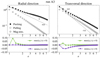 |
Fig. 5. Run A3. Evolution of the peaks of the dynamical terms with heliocentric distance, along x (left) and y (right). The peaks are computed inside the region of non-zero pinch tracer in order to filter out the shock fronts that propagate outwards. The top panels show the absolute value of the main terms: pushing and pulling terms are drawn with black and white filled circles, and magnetic tension with light grey circles; dotted black lines represent the predicted scaling laws for magnetic and kinetic pressure gradient terms as shown in Eq. (22). The bottom panels show the maximum and minimum of the resultant, in green and purple respectively. All the terms are in code units. |
Along the radial direction (left panels): for short distances the previous scaling analysis based on Eq. (22) seems to hold: magnetic tension is negligible, magnetic pressure dominates on the gas pressure, giving an outwards net acceleration that produces the radial expansion; at the same time, this same dynamical imbalance triggers a compression-rarefaction wave which enhances the gas pressure gradient, soon restoring the equilibrium which lasts for successive times.
Along the transversal direction (right panels): the initial dynamics is a bit more complex, with positive and negative accelerations (bottom panel) that cause a non homogeneous deformation of the flux rope. The dominant acceleration is the inward one, producing a less-than-kinematic transversal expansion. The magnetic tension contributes almost equally to the gas pressure in the pulling term at all distances. Eventually an equilibrium is reached as well.
3.3. Summary
The overall picture for a magnetic flux rope in a spherically expanding flow (exemplified with run A3) can then be summarised as follows:
-
The initial static and stationary equilibrium is perturbed by the anisotropic spherical expansion as the box is set in motion; the resulting dynamical imbalance produces accelerations in both directions: along the radial direction the flux rope is pushed away from its axis, whereas along the transversal direction it is pulled towards it;
-
Such forces produce local velocities which act on the plasma: they counteract the geometrical stretching and cause a radial expansion and a transversal contraction (or less than geometrical expansion);
-
After the initial dynamical phase, the system reaches an equilibrium configuration, with the local velocities still present: the radial expansion and transversal contraction remain while the box is being transported away from the Sun by the large-scale flow, and evolves through a series of successive equilibria.
3.4. Dependence of flux rope size on the expansion rate and plasma β
We now study how the radial and transverse sizes vary with the two non-dimensional parameters, the non-dimensional expansion rate ɛ0 and the effective plasma beta β0.
We first focus on the expansion rate. On the one hand the anisotropic spherical expansion perturbs the equilibrium on expansion timescales τexp. On the other hand, the flux rope reacts against perturbations on a timescale related to the in-plane Alfvén time τA. The non-dimensional expansion rate ɛ0 thus controls the relative importance of the continuous geometrical stretching (and its consequences on the decrease of gradients and fields) and of magnetic tension reactivity.
In Fig. 6 we plot flux rope size estimates, σx and σy, as a function of the heliocentric distance for runs A2-A6, that is, for increasing expansion rate ɛ0. The values of σx,y are rescaled to their initial value for better readability; σx and σy are coloured in shades of blue and orange respectively, with lighter shades representing higher expansion rates ɛ0; the trends expected from simple kinematic expansion are drawn as thick light lines of the same colours; run A3 discussed in the previous section is represented as a dash-dotted line. For higher expansion rates, at a given distance the transverse size gets larger, approaching the kinematic behaviour, whereas the radial size gets smaller but keeps its increasing trend even for the strongest expansion rate considered here.
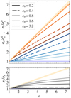 |
Fig. 6. Heliospheric evolution of the flux rope size estimates σx and σy (top panel) and the y-x aspect ratio (bottom panel) for runs A2, A3, A4, A5, and A6, that is, increasing ɛ0. Lighter shades represent increasing parameter values. Run A3 is represented as a dash-dotted line. The light blue (orange) broad line represents the expected ‘kinematic’ trend along x (y). |
Independently of the expansion rate, the trends of σx,y exhibit two stages: a first transient with variable slope, and a more stable phase with a more constant slope. This is consistent with the dynamical analysis shown in Fig. 5, with a first phase of dynamical imbalance and a second phase of expanding equilibrium; moreover, the transient lasts longer along y than along x, consistently with the persistence of net accelerations along the same directions. Finally, for higher expansion rates the variable transient lasts for a longer distance.
The aspect ratio σy/σx is also plotted versus distance in the bottom panel of Fig. 6, using shades of grey with the same meaning as in the top panel. A critical expansion rate  can be visually identified such that for
  (runs A2-A3) the aspect ratio attains an asymptotic value close to one (both directions continue to expand but at the same rate) whereas for
  (runs A4-A6) the aspect ratio continues to increase without reaching a constant value. Even for the highest expansion rate considered here, the kinematic trend of the aspect ratio is not reached because of the radial expansion.
The critical expansion rate can be estimated considering the 2D magnetic tension communication timescale between x and y: the azimuthal Alfvén speed is  , and it has to travel the length of a quarter-circle arc Lθ=πLFR/4; this implies that the effective expansion rate is

then ɛ0,eff≶1 corresponds to ɛ0≶(4/π)(Bθ,0/Bz,0) and with our choice of Bθ,0/Bz,0 = 1/2 we have  .
.
The different behaviour for runs with  can be understood by considering how the expansion rate evolves with distance. Following Eqs. (3), (7) and (8), the Alfvén timescales along the x and y direction both scale3 as τA∝a. The expansion timescale at a given distance can be estimated from Eq. (5b) and also scales as
  . Thus the non-dimensional expansion rate at any distance stays constant and only depends of its initial value:

This in turn implies that if ɛ0 is initially set greater (smaller) than  , then the flux rope will remain causally connected (or disconnected in some regions) during the expansion. In addition, simulations with different values of ɛ0 are not just shorter or longer portions of the same evolution, but intrinsically different ones.
By increasing the non-dimensional expansion rate, we are considering magnetic clouds that move (and are anisotropically stretched) faster and faster with respect to the timescales of their internal processes (e.g. Alfvén waves); a higher expansion rate implies a faster stretching, but also a stronger dynamical imbalance and thus more intense velocity fields; however, a faster magnetic cloud has also less time for its internal dynamics to develop, that is, for the internal velocities to act on the flux rope. In Fig. 7 we show the evolution of the maximum radial and minimum transversal velocities ( and
and  ) with time for different expansion rates;
  and
and  are directly related to radial expansion and to resistance to transversal expansion, respectively; the graphical conventions are the same as for Fig. 6. As the expansion rate increases (lighter lines),
  gets higher, but this increase is less than linear with ɛ0 (scales approximately as ɛ01/2); since the travel time for fixed initial and final distances scales as ɛ0−1 by definition, the result is a radial expansion which decreases for higher expansion rates. For the transversal velocity, the same reasoning applies, but the EBM frictional force further damps |uy|: the result is a weaker transversal resistance for higher expansion rates. Overall, these two effects imply that higher ɛ0 correspond to smaller deviations from the predicted kinematic evolution and a more elongated aspect ratio, explaining Fig. 6.
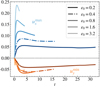 |
Fig. 7. Time evolution of the maximum of ux and minimum of uy (both computed across a 1D cut passing through the axis, as in Fig. 4) for runs A2-A6. The trends of |


In Fig. 8 we focus instead on the variation of the flux rope size associated with different plasma β0 (the graphical conventions are the same as in Fig. 6, this time lighter shades represent increasing β0 values). For increasing β0, both the radial and transversal sizes decrease (top panel) and the aspect ratio is essentially invariant (bottom panel); the ratio between magnetic tension and expansion timescales is kept constant, and a larger β0 implies an isotropic increase of the gas (external) pressure gradients, thus the size of the flux rope increases less, independently of the directions. However, radial expansion is clearly present even for run D3, which has β0∼4.
4. Results: Turbulent simulations
We now consider a flux rope that is not isolated but embedded in turbulent fluctuations that are added in the whole domain (including the flux rope itself).
4.1. Average and spectral quantities
In Fig. 9 we compare the temporal evolution of mean quantities for runs Y3h and Y3, the former having no expansion, the latter having the same ɛ0 = 0.4 as run A3. In each panel we plot the average sound speed 〈cs〉, the velocity and magnetic RMS fluctuations, the relative density RMS fluctuations, and the square of the current density 〈|J|2〉. Velocity and magnetic fluctuations are divided by the sound speed at each time, with magnetic fluctuations expressed in Alfvén units,  .
.
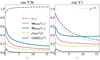 |
Fig. 9. Root mean square amplitude of fluctuations for runs Y3h (no expansion, left panel) and Y3 (ɛ0 = 0.4, right panel). Magnetic (green) and velocity (red) fluctuations are normalised to the average sound speed (magnetic fluctuations are expressed in Alfvén units before normalisation, see text), while density fluctuations (light green, dash-dotted) are normalised to the average density. The average sound speed and the square of the current density are also plotted with purple and black dashed lines, respectively. In the right panel, the predicted a−2/3 decay for sound speed is drawn as a grey dotted line. |
We consider first the non expanding case (left panel). Despite the presence of the flux rope, fluctuations are almost at equipartition at the initial time. Since fluctuations are initially excited at relatively large wave-numbers, turbulence develops very quickly and intense small-scale currents form very soon (recall χ≫1) and heat the plasma. Hence the rapid decay of the normalised velocity and magnetic fluctuations is due to both the development of turbulence that drains energy from fluctuations and to the increase of the sound speed. At later times t≳5, turbulence slows down, turbulent dissipation decreases, fluctuations decay more gently, and the sound speed only slightly increases. Fluctuations are subsonic initially and remain largely subsonic at later time, with δu/cs ≳δρ/〈ρ〉.
When expansion is switched on (right panel), the evolution at early times remains basically unchanged. In other words, the development of turbulence in response to the out-of-equilibrium initial conditions is the same and more rapid than the effects of expansion (recall ɛT≪1). Both the average density and temperature decrease according to Eqs. (7) and (10), and the plasma heating now shows up as an initial less-than-adiabatic decrease of the sound speed. After the initial phase, the sound speed follows an adiabatic decrease (grey dotted line), and the level of (normalised) velocity, magnetic, and density fluctuations settles to an approximately constant value that is larger than in the homogeneous case. Thus, velocity and magnetic fluctuations (the latter in Alfvén units) decay approximately as a−2/3, while density fluctuations as a−2. A small magnetic excess continues to develop at later times, possibly because of the persistence of the flux rope magnetic field.
For the expanding simulation Y3, the evolution of the omnidirectional spectra of velocity and magnetic fluctuations are shown in Fig. 10, the latter again expressed in Alfvén units, with lighter colours indicating successive times: t = 0.0,4.0,8.0,12.0,16.0, which correspond to an increase of the distance and transverse size up to a factor 7.4. In the plot, the abscissa is further normalised to the smallest wave-number, k0 = 2π/Lx, which is the same at all times. Initially (black line), the spectrum of velocity is flat and made of turbulent fluctuations only, while the magnetic field spectrum clearly shows the flux rope energy at k≤6. In both panels the secular decay due to the EBM frictional forces is apparent, with spectra decreasing as a whole at successive times, and faster for u than for b (cf. Eqs. (9)–(8)). Velocity fluctuations of small amplitude develop at large scales (k/k0≲6), while in the magnetic field spectrum this range is dominated by the flux rope that remains as a distinguishable feature at all times. At smaller scales, 15≲k/k0≲70, an inertial range develops with a power-law range, with a spectral slope slightly steeper than −5/3 for u and slightly steeper than −2 for b. In the magnetic spectrum the boundary between the flux rope and turbulent fluctuations at k/k0≈6 is smoothed out for large distances; this suggests a cross-scale interaction between turbulent vortexes and the flux rope. Finally, for larger wave-numbers the spectra drop significantly because of the stretching of the domain: at t = 4 the largest transverse wave-vector is  , and in the last spectrum it further reduces to
  . In other words, as the distance increases the omnidirectional spectra at the smallest scales are made mainly of radial wave-vectors.
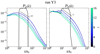 |
Fig. 10. Omnidirectional spectra of velocity and magnetic field (Eq. (19)) as a function of the normalised wave number for run Y3. Different times are shown as indicated in the colour bar. The spectrum corresponding to the flux rope is visible at k/k0≲6 in the magnetic spectrum. |
4.2. Radial expansion and ageing of turbulence
We now focus on the evolution of run Y3 in real space: the heliocentric evolution of the magnetic field intensity and field lines for run Y3 is shown in Fig. 11 with the same style and conventions as Fig. 3. The snapshots are taken at the same times of the omnidirectional spectra and span the whole duration of the simulation (unlike Fig. 3 which only covered t≤8.0), that is, t = 0.0,4.0,8.0,12.0,16.0 and a final domain stretching of 7.4. For better visual representation, |B| is compensated by a3/2 and the 2D maps only show a portion of the domain, x∈(−2.5,+2.5) and y∈(−8.5,+8.5), with the actual domain boundaries being located at x=±4 at all times, and at y=±14.8 at the final time. The random fluctuations quickly interact to form currents and turbulent vortexes that are about one third of the flux rope size in this initial phase. Turbulent vortexes are expanding as well and lose energy because of the turbulent cascade, so that on average their size decreases with respect to the flux rope. Around the boundaries of the flux rope (especially the radial ones) a number of small scale structures form that have isotropic shapes (e.g. vortex-like structures on the left) or vertical elongation (e.g. sheet-like structures on the right). Comparison of the total magnetic field (colour map) and in-plane magnetic field (black iso-contour) also reveals that the out-of-plane Bz is more intense in vortexes that are close to the flux rope's vertical edge. Since 2D turbulence is unlikely to develop a strong out-of-plane magnetic field, this must originate from the diffusion and/or transport of the axial field of the flux rope (for example in the small blob on the top left corner of the flux rope). We come back to this point later in this section.
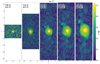 |
Fig. 11. Snapshots for successive times of the magnetic field for run Y3. The total magnetic field |B| is represented by the colour-coded map, and the in-plane magnetic field is shown with constant-Az black lines. Only a portion of the domain is shown, see text. |
The most striking fact emerging from Fig. 11 is that despite the strong turbulent field, the core of the flux rope remains clearly visible as the most intense magnetic field; as in the isolated case, the flux rope radial size grows, and its transverse size grows less than geometrically. We expect departures from the isolated case to be controlled by the age of expanding turbulence, or its inverse ɛT. In Fig. 12 we compare the final state (t = 16.0) of two runs with different ɛT: run Y3k with ɛT = 0.03 in the top row, and run Y3 with ɛT = 0.12 in the bottom row. The in-plane magnetic field intensity Bpl=(Bx2+By2)1/2 is shown in the left column, whereas the radial and transversal velocities ux and uy are shown in the central and right columns, respectively. In all panels, the pinch tracer is shown as a solid black line to indicate the flux rope boundaries; again, only a portion of the domain is shown for better visualisation. Let us focus on run Y3k (top panels) first. The in-plane magnetic field shows turbulent fluctuations that are filamented and about 10 times smaller in size and about 5 times smaller in amplitude than the flux rope field. The flux rope, as identified by the pinch tracer, is well bounded by the in-plane magnetic field in the radial direction. Instead, in the transverse direction its material is spread vertically, possibly because of diffusion outside the region bounded by magnetic tension. In the top right and central panels, the velocity profiles causing radial expansion and transversal contraction can be recognised as in Fig. 3. In addition, the vertical flows cause velocity shears uy(x) at the radial edges of the flux rope that in turn lead to an enhancement of the in-plane magnetic field, clearly visible in the top left panel. Summarising, at late times the kinematics is similar to the isolated case (run A3, Fig. 3 (b) and (c)) and turbulent fluctuations add a little perturbation to the flux rope structure. This is consistent with its ɛT≪1: the eddy turnover time is initially much shorter than the expansion time, so turbulence decays quickly and at later times few energy is left to perturb the flux rope, and the geometrical stretching forces the weakly interacting eddies into filamentary shapes.
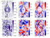 |
Fig. 12. Maps of the in-plane magnetic field, |
The situation is different for our fiducial case, run Y3 (bottom panels of Fig. 12). Turbulent fluctuations have a magnetic field intensity comparable to that of the flux rope, their size is relatively large (about 1/3 of the flux rope), and have mainly vortex-like shapes. A central core forms well inside the flux rope material identified by the tracer, and is surrounded by magnetic field enhancements at the flux rope edges. As before, dispersion in the vertical direction takes the form of filamentary structures at the top and bottom edges, but also vortex-like structures are present (e.g. in the top left corner). In the middle and right panels, the turbulent δux,y are comparable in size and magnitude to those of the flux rope, with clear vortex-like patterns. The ratio ɛT≲1 indicates that turbulence is dynamically relevant also at late times. The central core of the flux rope rotates counter-clock wise, while now velocity shears appear at both the radial and transverse edges. While it is clear that the transverse component of velocity has lost its dipolar structure at the vertical edges (right panel of Fig. 12), with the aid of the tracer in the middle panel one can recognise a profile of the radial velocity ux(x) resembling the unperturbed case. Thus, large-scale and large-amplitude turbulence is effective in perturbing the flux rope structure and dynamics along the transverse directions. Along the radial direction, the flux rope maintains approximately the radial velocity profile that was found in the isolated case and that defines radial expansion. Clearly both χ and ɛ0 control the impact of turbulence on the flux rope equilibrium and suggest that values of ɛT closer to unity are more effective in perturbing the flux rope equilibrium; a better handle on the final state is obtained by controlling separately kturb/kFR and δB/Bθ,0.
4.3. Magnetic field dispersion and size estimates
We now focus on the causes of the dispersion of the flux rope material in the vertical direction, and in particular on the role of transport and magnetic diffusion. On the one hand, transport is possible without diffusion because our initial equilibrium has a non-negligible axial field beyond the flux rope pinch (see Sect. 2.3 and Fig. 2). On the other hand, velocity maps display clear signatures of magnetic reconnection between the field of the flux rope and that of the vortexes (we note however that this process could be amplified by the presence of strong turbulent fluctuations inside the flux rope, arbitrarily set to δB/Bθ,0 = 1 in this work). To clarify the importance of both effects we compare in Fig. 13 the intensity map of the axial magnetic field at the final time for runs A3, Z3, and Y3, which correspond to an isolated case, a turbulent case with weaker fluctuations inside the flux rope, and uniform fluctuations, respectively. For easier comparison with the last panel in Fig. 11, on the colour map we superpose the iso-contour of the in-plane magnetic field with black lines; moreover, to identify the flux rope material, we draw the boundary of the pinch and the axial tracers in the top and bottom panels, respectively. We recall that the pinch tracer is initially limited to the region bounded by the in-plane magnetic field, while the axial tracer extends further out in the vertical direction to cover also the out-of-plane flux rope magnetic field (see Figs. 2 and 3).
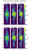 |
Fig. 13. Snapshot at t = 16.0 (a = 7.4) of the magnetic field for runs A3 (isolated flux rope), Z3 (with fluctuations smaller inside the flux rope by a factor 5), and Y3 (with equal fluctuation amplitude everywhere). The axial field Bz is represented by the colour-coded map, whereas the in-plane magnetic field is represented with constant-Az black lines. The two rows show the same fields (colour map and black iso-contours) but differ for the tracer, which is plotted with a thick white line: in the top row, we show the pinch tracer that is initially co-spatial with the in-plane (poloidal) magnetic field; in the bottom row, the white lines bound the axial tracer that is initialised in the same region occupied by the out-of-plane (axial) magnetic field. |
We first focus on the isolated case (left column). The axial field Bz extends well beyond the pinch tracer but is well bounded by the axial tracer. This axial field is transported away from the flux rope in the vertical direction because the plasma that initially lies outside the in-plane flux rope field is freely stretched in that direction without the restoring force provided by the magnetic tension. Thus, no magnetic diffusion is at work in the isolated case. When turbulent fluctuations are present, but with a smaller amplitude inside the flux rope than outside of it (middle panels), the axial field has a similar vertical extent, a more irregular pattern due to the turbulent motions, and about the same intensity. Now, the pinch tracer covers most of the axial field in the vicinity of the flux rope; this indicates that such intense Bz originates from diffusion (reconnection) and subsequent transport. Finally, the right panels show that if turbulent fluctuations are more intense inside the flux rope, diffusion is more effective and intense Bz can be transported further away, reaching distances comparable to the flux rope size. In the radial direction the two tracers are basically co-spatial; this indicates that reconnection and transport are effective only in the transverse direction.
Finally, we show the heliocentric evolution of radial and transverse sizes as measured with the pinch tracer for the turbulent runs, with run A3 as a reference. In Fig. 14 we plot again σx and σy as a function of distance for runs A3 (loosely dash-dotted), Y3k (densely dash-dotted), Y3 (dotted) and Z3 (dashed), with the same colour notation as in Fig. 6. As anticipated, the increase of the radial size is basically unchanged (all the lines are very close to each other): turbulence has a little effect despite its δB≈Bθ,0 and irrespective of the internal level of turbulence. On the contrary, the transverse size of the flux rope is strongly affected when the turbulence is durable (runs Y3 and Z3, dotted and dashed lines), and approaches the kinematic trend σy∝a in the more extreme case of run Y3; on the contrary, the short-lived turbulence of run Y3k shows little variation. We note, however, that the measure of the flux rope size, σx (σy), is obtained by averaging in the y (x) direction, thus it smears out the differences that are instead visible in the 2D maps of Fig. 13 and could be grasped by cutting the structure at its centre (which is more similar to what a spacecraft might see).
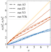 |
Fig. 14. Heliospheric evolution of the pinch tracer sizes (σx and σy) for runs A3 (no turbulence, dash-dotted line), Z3 (turbulence out greater than in, dashed line), Y3 (turbulence in and out, dotted line), and Y3k (turbulence in and out at smaller scales, densely dash-dotted line). The light blue (orange) broad line represents the expected ‘kinematic’ trend along x (y). |
5. Comparison with previous works and discussion
5.1. General features and comparison at 1AU
Our simulations naturally reproduce a configuration with a flux rope at a lower temperature than the surrounding solar wind of the same velocity (one of the main observational signatures of magnetic clouds, see e.g. Richardson & Cane 1995), and a decreasing plasma β inside the flux rope with heliocentric distance. The rarefaction (cooling) wavefront produced by the dynamical imbalance inside the flux rope accounts for the former, whereas the latter can be explained as a superposition of the spherical decay (magnetic pressure decreasing less than kinetic pressure) and the local advection motions (radial expansion) which stretch the magnetic field profile.
Previous studies (Démoulin et al. 2008; Démoulin & Dasso 2009; Gulisano et al. 2010) usually found the different heliocentric scaling laws of magnetic and kinetic pressures to be the main culprit for the radial expansion; while this remains true for our analysis, our results suggest that the anisotropy and spatial dilation due to the spherical nature of solar wind flow also play a role: they imply different behaviours for radial and transversal directions (affecting the section's final aspect ratio) and depend on the ratio between internal and external timescales (controlled here by the non-dimensional expansion rate ɛ0).
To relate our non-dimensional expansion rate ɛ0 to actual flux ropes and to compare our results to observed quantities at 1 AU, we choose as a reference the superposed epoch analysis at 1 AU reported in Salman et al. (2020a), Table 1, ‘Cat-III’ set (CMEs with no sheath, closer to our assumption of constant propagation speed). To obtain dimensional values from our runs, we fix the dimensional units at R0 = 30 R⊙: the flux rope axial field B0=BFR = 120 nT, the (uniform) mass density ρ0=ρbg = 236mp cm−3 and the initial flux rope width L0=LFR = 0.05 AU. This leaves ɛ0 to be determined from the (constant) propagation speed U0, or vice versa. For runs A3 and A6 we fix U0 using the respective values of ɛ0 indicated in Table 1; then we also consider one more simulation, run AR, for which we choose U0≃466 km/s (average of the leading edge speeds distribution traced up to 32 R⊙, from Gopalswamy et al. 2010) which implies ɛ0 = 1.0. If we considered all the dimensional parameters to be fixed except from U0, then the range of values of ɛ0 used in this study would correspond to constant radial speeds U0∼90 km/s to 1500 km/s. It should be stressed once more that these are just examples: the same value of ɛ0 can describe very different magnetic clouds, but at the same time two extremely similar magnetic clouds with different ejection speeds will have very different values of ɛ0.
Table 2 shows in the first row our reference, and in the other rows the results from our runs. We get values lower than average for magnetic field, density and radial size, and a higher than average plasma β; most of our estimates seem to fall within the standard deviations; a particularly good agreement is found for the expansion velocities, whereas the propagation velocity is clearly out of range because we assumed it constant. The higher 〈β〉 and the smaller radial extent might be attributed to our limitations on the values of β0 (see the next section for a further comment).
Comparison between averages based on a superposed epoch analysis at 1 AU (Salman et al. 2020a, Table 1, ‘Cat-III’ set) and our runs A3, AR, and A6, which correspond to different values of the non-dimensional expansion rate ɛ0.
5.2. Dimensionless estimates of radial expansion
Given the large variability of flux rope parameters, we can instead focus on dimensionless estimates. From our trends of σx(a) we can directly estimate the heliocentric scaling exponent of the flux rope's radial size, αR, defined such that S∝RαR, which is shown together with the trends in Fig. 15. The σx(a) we observe is made of an initial transient phase, which coincides with the span of non-zero radial dynamical imbalance (cf. the bottom left panel of Fig. 5) and whose duration in heliocentric coordinate depends on ɛ0 (Fig. 6), and of a second asymptotic linear phase. Because of the dynamical transient with little to no radial expansion, the effective scaling exponent is necessarily lower than its asymptotic value. To consider only the latter phase of constant radial expansion, we fix the fitting interval as a>2 (R>0.29 AU); this works very well for runs A2-A3, but we still get a transitional phase for runs A4-A6, which leads to a systematic underestimation of αR. Using this range, we find αR = 0.78 to 0.41 for runs A2 to A6 (ɛ0 = 0.2 to 3.2), which indicates a clear anti-correlation between αR and ɛ0. As was expected from visual inspection of Fig. 6, αR<1 for all the considered cases. We also draw as a grey shaded area the envelope between minimum and maximum slope obtained by randomly collecting 10 samples from each run and using the ensemble to perform a ‘statistical’ power-law fit, repeating for several random pickups. We can see that, based on which points we pick (i.e. on where we sample the different ‘events’) the asymptotic slopes of single kinds of CMEs can be under or overestimated, possibly overestimating our highest αR (consistently with previous discussions, e.g. in Salman et al. 2024). Most of our values of αR are consistent with previous works, such as 0.78±0.10 (Bothmer & Schwenn 1998), 0.92±0.07 (Liu et al. 2005), 0.61±0.09 (Leitner et al. 2007), 0.78±0.12 (Gulisano et al. 2010), even though they fall on the lower end.
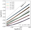 |
Fig. 15. Heliospheric evolution of the flux rope radial size S[AU] versus distance R[AU] for runs A2-A6. Only the range a>2 (R>0.29 AU) is considered, to avoid the first dynamical transient for most runs (even though it is still visible and important in runs A4-A6). The estimates of S using σx are drawn as markers (different shapes for different runs), and each run has been fitted with a power law (solid lines with different colours). The solid thin black line is the linear (αR≡1) trend. The shaded grey area highlights the range between the minimum and maximum αR values obtained by randomly sampling data points from the combined set of runs A2-A6 (see text for details). |
We also extract from our radial velocity profiles at 1 AU the non-dimensional expansion parameter ζ, which gives a local estimate of the radial expansion exponent, and is defined following Gulisano et al. (2010):

which, in our framework, is computed as

where Δx=xfront−xback and Δux is the corresponding radial velocity difference.
The values of ζ estimated from runs A2-A6 at 1 AU are shown in Fig. 16 together with the 1D radial profiles of local radial velocity (bottom panel) and total magnetic field (top panel) obtained by cutting through the axis; this also shows once more that the radial velocity peak acts on the edge of the flux rope. We find ζ = 0.85 to 0.49 for runs A2 to A6 (ɛ0 = 0.2 to 3.2), anti-correlated to ɛ0 similarly to αR. Moreover, for weaker expansion rates the final magnetic field is less intense and more spread, whereas for stronger expansion rates the magnetic field is more intense and compact; this can be easily seen comparing for example run A2 (ɛ0 = 0.2, blue lines) with run A6 (ɛ0 = 3.2, violet lines). These values are positively correlated to the values of αR discussed above; in particular, we find αR≲ζ for all our runs, meaning that at least for our conditions the local measure of expansion based on the velocity slope (ζ) seems to overestimate the actual heliocentric scaling exponent of the radial size of the flux rope (αR). We note that an intrinsic anti-correlation exists between ζ and ɛ0 by definition in Eq. (25), but the same reasoning as Sect. 3.4 holds: the radial expansion velocity scales more weakly with ɛ0 than does the available time. The range of ζ values we obtain for different EBM expansion rates is roughly consistent with the observational estimates of 0.81±0.19 by Démoulin (2010) and 0.91±0.23 by Gulisano et al. (2010), although we fall again on the lower end ζ≲0.8.
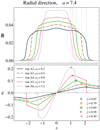 |
Fig. 16. Total magnetic field intensity |B| (top panel) and radial velocity ux (bottom panel) for runs A2-A6, along a radial cut through the flux rope axis, for the final times (R≃1 AU). In the bottom panel, the peak of ux is drawn with markers (the same as in Fig. 15 for each run) and labelled with the corresponding estimate of the non-dimensional expansion parameter ζ; the position corresponding to the peak is drawn as a light dashed vertical line in the top panels, to compare it to the magnetic boundaries. Run A3 is shown as a dash-dotted line in both panels. |
Finally, the flux rope's peak magnetic field intensity follows a heliocentric power-law decay |B|max∝RαB with exponent αB=−1.66 to −1.49 for runs A2 to A6 (ɛ0 = 0.2 to 3.2); the range is quite narrow and the values are again anti-correlated with ɛ0: higher expansion rates imply a slower magnetic field decay, as can be seen in the top panel of Fig. 16. The validity of |αB|/2 as a proxy for αR appears to be better for lower values of ɛ0 (i.e. tA≪texp). Our values of αB for |B|max are consistent with previous works based on observations, such as −1.64±0.40 (Leitner et al. 2007), −1.34±0.71 (Good et al. 2019), −1.41±0.49 (Vršnak et al. 2019), −1.91±0.25 (Salman et al. 2020b), −1.81±0.84 (Lugaz et al. 2020), −1.67±0.88 (Zhuang et al. 2023).
6. Conclusions
6.1. Summary and main results
In this study we performed MHD numerical simulations using the EBM to study the heliospheric evolution of the 2.5D section of a magnetic flux rope propagating with the spherically expanding solar wind. We first considered the flux rope in the spherical solar wind flow only, and varied two control parameters: the non-dimensional expansion rate, ɛ0 (how fast the flux rope propagates compared to its internal Alfvén times), and the effective plasma beta, β0 (how energetic the flux rope is compared to the environment).
With its intrinsic anisotropy, the spherical flow perturbs the flux rope, which reacts and develops a local dynamics: its radial size grows (action of magnetic pressure) and its transversal size resists spherical stretching (action of magnetic tension). The system eventually reaches a series of successive equilibria that include the local flows.
Stronger expansion rates imply a more dominant magnetic pressure but also faster transit and stretching, which results in a less effective internal dynamics, a more elongated aspect ratio, and an evolution close to spherical expansion. Lower beta values imply isotropically larger sizes because of the more predominant magnetic pressure. The internal dynamics is thus relevant especially for low β and weak expansion rates ɛ0=tA/texp<1.
In the relevant case of weak expansion, we also superposed turbulent fluctuations on the isolated configuration, introducing another timescale, the non-linear time, tNL. The transversal resistance to stretching is strongly affected, whereas the radial size growth is almost unaltered. The turbulent shearing and distorting motions transport the plasma (especially where magnetic tension is weaker), produce secondary structures, and shape the flux rope at small scales. Turbulence is only effective in perturbing the flux rope when it is long-lived with respect to the expansion timescale; energetic but short lived fluctuations have little effect. We suggest turbulence to be relevant when ɛT=tNL/texp≲1.
We validated our simulations by comparing the results to a superposed epoch analysis at 1 AU (Salman et al. 2020a, Table 1, ‘Cat-III’ set), and found a quite good agreement. However, in our simulations we underestimate plasma parameters such as density, magnetic field intensity, and radial size (see Table 2), probably due to our parameter limitations. We also estimated the non-dimensional expansion parameter, ζ, from the radial expansion velocity, and the radial size scaling exponent, αR, from the radial size increase with distance S∝RαR. We find such local and global radial expansion estimates to be comparable, and both clearly anti-correlated with our non-dimensional expansion rate, ɛ0. The peak magnetic field scaling exponent, αB, seems to work well as a proxy for αR (especially when tA≪texp). Estimating αR from a set of position-size data points randomly sampled from different simulations clearly masks the single events, and can even overestimate (underestimate) the strongest (weakest) radial expansion exponent, just because of chance.
Our results seem consistent with the widely accepted view that explains the radial expansion of magnetic clouds through the imbalance between magnetic and kinetic pressures (e.g. Démoulin & Dasso 2009). However, this work gives more details on the internal dynamical processes and shows that radial expansion survives in the presence of turbulence.
We stress that the dynamical imbalance that produces radial expansion in our simulations would still arise for different kinds of initial configurations: a purely magnetic force-free equilibrium would have different scaling laws for magnetic pressure and tension, and a pressure-confined axial flux tube (no magnetic tension) would have different scaling laws for magnetic and kinetic pressures. This kind of evolution is thus a direct consequence of the solar wind's spherically expanding geometry. We expect our results to be mainly valid for magnetic clouds without shock fronts, that is, those which propagate at velocities close to the ambient solar wind.
6.2. Limitations and perspectives
Our estimates of the radial size scaling exponent and the non-dimensional expansion parameter both fall in the lower end of the ranges that come from observations (see Sect. 5); both also show a less than linear (∝R) expansion; this might be due to our limited β range related to our choice of initial condition (see Sect. 2.3). Since the radial expansion effect increases in our simulations for decreasing β0 (see Sect. 3.4), we expect our results to approach the upper end of the observed values when we have lower β0 values.
Furthermore, assuming that the flux rope remains unperturbed at the starting radial position R0 = 30 R⊙ is probably not very realistic. We might be overestimating the duration of the dynamically imbalanced phase compared to the transit time, which means underestimating the duration of the successive phase of constant radial expansion, overall obtaining a radial size smaller than average at 1 AU.
Moreover, even though we fixed the helical twist parameter of our initial configuration by arbitrarily fixing Bθ,0/Bz,0 = 1/2, we expect flux ropes with different degrees of twist to have a different evolution (final radial size and aspect ratio) because of the different magnetic pressure-to-tension ratio, which introduces an additional parameter. A 3D extension of this study is probably needed to more completely assess such a dependence. The estimate of an EBM-like expansion parameter, ɛ0 (or its version considering the helical twist ɛ0,eff, see Sect. 3.4) for multiple in-situ magnetic clouds might be assessed in a subsequent study and would provide a further test for the general validity of our results.
Finally, the interaction with the interplanetary magnetic field and the presence of a velocity difference with solar wind, both neglected here, are expected to (strongly) perturb the evolution described in this work. The former would probably erode the magnetic cloud as it expands, also adding magnetic pressure all around it; the latter would likely produce a shock front and a sheath region that would also spark additional dynamics and higher dynamical pressure gradients, which might compress the flux rope in the radial direction and produce the well-known ‘pancaking’ effect.
Acknowledgments
We acknowledge partial financial support from the European Union – Next Generation EU – National Recovery and Resilience Plan (NRRP) – M4C2 Investment 1.4 – Research Programme CN00000013 “National Centre for HPC, Big Data and Quantum Computing” – CUP B83C22002830001 and by the European Union – Next Generation EU – National Recovery and Resilience Plan (NRRP) – M4C2 Investment 1.1- PRIN 2022 (D.D. 104 del 2/2/2022) – Project “Modeling Interplanetary Coronal Mass Ejections”, MUR code 31. 2022M5TKR2, CUP B53D23004860006. We acknowledge the CINECA award under the ISCRA initiative, for the availability of high performance computing resources and support from the Class C project TUCME, “Turbulent evolution of Coronal Mass Ejections”, code HP10C29IHP (PI: M. Sangalli). M. S. wishes to thank S. Antiochos for useful comments on an early presentation of this work; the authors also wish to thank L. Del Zanna for useful discussions. The authors wish to thank the referee for their comments which helped improve the manuscript.
Other dynamical terms arise after the first dynamical phase, in addition to the ones considered so far: mainly the advection −u·∇u and, along y, the EBM-related frictional deceleration  . Therefore, the total acceleration is not everywhere zero (cf. the inset in panel (c) of Fig. 4).
Actually, the effective timescale for the 2D communication mediated by magnetic tension would be better estimated as the time it takes for an Alfvén wave to travel along the elliptical arc of angular width π/2, varying minor and major axes LFR,x and LFR,y, with varying speeds cA,x and cA,y. It can however be approximated as τA∝a.
References
- Ala-Lahti, M., Ruohotie, J., Good, S., Kilpua, E. K. J., & Lugaz, N. 2020, J. Geophys. Res. (Space Phys.), 125, e2020JA028002 [Google Scholar]
- Borovsky, J. E., Denton, M. H., & Smith, C. W. 2019, J. Geophys. Res. (Space Phys.), 124, 2406 [Google Scholar]
- Bothmer, V., & Schwenn, R. 1998, Ann. Geophys., 16, 1 [Google Scholar]
- Bruno, R., & Carbone, V. 2013, Liv. Rev. Sol. Phys., 10, 2 [Google Scholar]
- Burlaga, L. F. 1988, J. Geophys. Res., 93, 7217 [NASA ADS] [CrossRef] [Google Scholar]
- Démoulin, P. 2010, in Twelfth International Solar Wind Conference, eds. M. Maksimovic, K. Issautier, N. Meyer-Vernet, M. Moncuquet, & F. Pantellini, AIP Conf. Ser., 1216, 329 [Google Scholar]
- Démoulin, P., & Dasso, S. 2009, A&A, 498, 551 [Google Scholar]
- Démoulin, P., Nakwacki, M. S., Dasso, S., & Mandrini, C. H. 2008, Sol. Phys., 250, 347 [Google Scholar]
- Dong, Y., Verdini, A., & Grappin, R. 2014, ApJ, 793, 118 [Google Scholar]
- Frigo, M., & Johnson, S. G. 2005, IEEE Proc., 93, 216 [Google Scholar]
- Goldstein, M. L., Roberts, D. A., & Matthaeus, W. H. 1995, ARA&A, 33, 283 [NASA ADS] [CrossRef] [Google Scholar]
- Good, S. W., Kilpua, E. K. J., LaMoury, A. T., et al. 2019, J. Geophys. Res. (Space Phys.), 124, 4960 [NASA ADS] [CrossRef] [Google Scholar]
- Good, S. W., Ala-Lahti, M., Palmerio, E., Kilpua, E. K. J., & Osmane, A. 2020, ApJ, 893, 110 [NASA ADS] [CrossRef] [Google Scholar]
- Good, S. W., Rantala, O. K., Jylhä, A. S. M., et al. 2023, ApJ, 956, L30 [Google Scholar]
- Gopalswamy, N., Akiyama, S., Yashiro, S., & Mäkelä, P. 2010, in Magnetic Coupling between the Interior and Atmosphere of the Sun, eds. S. S. Hasan, & R. J. Rutten, Astrophys. Space Sci. Proc., 19, 289 [Google Scholar]
- Gosling, J. T., Hildner, E., MacQueen, R. M., et al. 1975, Sol. Phys., 40, 439 [Google Scholar]
- Gosling, J. T., McComas, D. J., Phillips, J. L., & Bame, S. J. 1991, J. Geophys. Res, 96, 7831 [Google Scholar]
- Grappin, R., & Velli, M. 1996, J. Geophys. Res., 101, 425 [NASA ADS] [CrossRef] [Google Scholar]
- Grappin, R., Velli, M., & Mangeney, A. 1993, Phys. Rev. Lett., 70, 2190 [NASA ADS] [CrossRef] [Google Scholar]
- Gulisano, A. M., Démoulin, P., Dasso, S., Ruiz, M. E., & Marsch, E. 2010, A&A, 509, A39 [NASA ADS] [CrossRef] [EDP Sciences] [Google Scholar]
- Huttunen, K., & Koskinen, H. 2004, Ann. Geophys., 22, 1729 [NASA ADS] [CrossRef] [Google Scholar]
- Jian, L. K., Russell, C. T., Luhmann, J. G., Skoug, R. M., & Steinberg, J. T. 2008, Sol. Phys., 250, 375 [Google Scholar]
- Kataoka, R., Watari, S., Shimada, N., Shimazu, H., & Marubashi, K. 2005, Geophys. Res. Lett., 32, L12103 [Google Scholar]
- Kennel, C. F., Scarf, F. L., Coroniti, F. V., Smith, E. J., & Gurnett, D. A. 1982, J. Geophys. Res., 87, 17 [Google Scholar]
- Kilpua, E., Koskinen, H. E. J., & Pulkkinen, T. I. 2017, Liv. Rev. Sol. Phys., 14, 5 [Google Scholar]
- Kilpua, E. K. J., Fontaine, D., Good, S. W., et al. 2020, Ann. Geophys., 38, 999 [NASA ADS] [CrossRef] [Google Scholar]
- Klein, L. W., & Burlaga, L. F. 1982, J. Geophys. Res., 87, 613 [Google Scholar]
- Kumar, A., & Rust, D. M. 1996, J. Geophys. Res., 101, 15667 [Google Scholar]
- Leamon, R. J., Smith, C. W., & Ness, N. F. 1998, Geophys. Res. Lett., 25, 2505 [Google Scholar]
- Leitner, M., Farrugia, C. J., Möstl, C., et al. 2007, J. Geophys. Res. (Space Phys.), 112, A06113 [Google Scholar]
- Lepping, R. P., Berdichevsky, D. B., Szabo, A., Arqueros, C., & Lazarus, A. J. 2003, Sol. Phys., 212, 425 [Google Scholar]
- Lepping, R. P., Wu, C. C., Berdichevsky, D. B., & Ferguson, T. 2008, Ann. Geophys., 26, 1919 [Google Scholar]
- Liu, Y., Richardson, J. D., & Belcher, J. W. 2005, Planet. Space Sci., 53, 3 [Google Scholar]
- Lugaz, N., Farrugia, C. J., Winslow, R. M., et al. 2018, ApJ, 864, L7 [NASA ADS] [CrossRef] [Google Scholar]
- Lugaz, N., Salman, T. M., Winslow, R. M., et al. 2020, ApJ, 899, 119 [Google Scholar]
- Manchester, W., Kilpua, E. K. J., Liu, Y. D., et al. 2017, Space Sci. Rev., 212, 1159 [Google Scholar]
- Manoharan, P. K., Kojima, M., Gopalswamy, N., Kondo, T., & Smith, Z. 2000, ApJ, 530, 1061 [NASA ADS] [CrossRef] [Google Scholar]
- Márquez Rodríguez, R., Sorriso-Valvo, L., & Yordanova, E. 2023, Sol. Phys., 298, 54 [Google Scholar]
- Montagud-Camps, V., Grappin, R., & Verdini, A. 2018, ApJ, 853, 153 [NASA ADS] [CrossRef] [Google Scholar]
- Odstrcil, D., Riley, P., & Zhao, X. P. 2004, J. Geophys. Res. (Space Phys.), 109, A02116 [Google Scholar]
- Papini, E., Franci, L., Landi, S., et al. 2019, ApJ, 870, 52 [NASA ADS] [CrossRef] [Google Scholar]
- Papini, E., Cicone, A., Franci, L., et al. 2021, ApJ, 917, L12 [Google Scholar]
- Patsourakos, S., Vourlidas, A., & Kliem, B. 2010, A&A, 522, A100 [NASA ADS] [CrossRef] [EDP Sciences] [Google Scholar]
- Pezzi, O., Trotta, D., Benella, S., et al. 2024, A&A, 686, A116 [NASA ADS] [CrossRef] [EDP Sciences] [Google Scholar]
- Pomoell, J., & Poedts, S. 2018, J. Space Weather Space Clim., 8, A35 [NASA ADS] [CrossRef] [EDP Sciences] [Google Scholar]
- Rappazzo, A. F., Velli, M., Einaudi, G., & Dahlburg, R. B. 2005, ApJ, 633, 474 [NASA ADS] [CrossRef] [Google Scholar]
- Regnault, F., Janvier, M., Démoulin, P., et al. 2020, J. Geophys. Res. (Space Phys.), 125, e28150 [NASA ADS] [Google Scholar]
- Richardson, I. G., & Cane, H. V. 1995, J. Geophys. Res., 100, 23397 [Google Scholar]
- Richardson, I. G., & Cane, H. V. 2012, J. Space Weather Space Clim., 2, A01 [Google Scholar]
- Ruzmaikin, A., Feynman, J., & Smith, E. J. 1997, J. Geophys. Res., 102, 19753 [Google Scholar]
- Sachdeva, N., Subramanian, P., Colaninno, R., & Vourlidas, A. 2015, ApJ, 809, 158 [NASA ADS] [CrossRef] [Google Scholar]
- Salman, T. M., Lugaz, N., Farrugia, C. J., et al. 2020a, ApJ, 904, 177 [NASA ADS] [CrossRef] [Google Scholar]
- Salman, T. M., Winslow, R. M., & Lugaz, N. 2020b, J. Geophys. Res. (Space Phys.), 125, e27084 [NASA ADS] [Google Scholar]
- Salman, T. M., Nieves-Chinchilla, T., Jian, L. K., et al. 2024, ApJ, 966, 118 [NASA ADS] [CrossRef] [Google Scholar]
- Sheeley, N. R. J., Howard, R. A., & Michels, D. J., et al. 1985, J. Geophys. Res., 90, 163 [Google Scholar]
- Sorriso-Valvo, L., Yordanova, E., Dimmock, A. P., & Telloni, D. 2021, ApJ, 919, L30 [NASA ADS] [CrossRef] [Google Scholar]
- St. Cyr, O. C., Plunkett, S. P., & Michels, D. J., et al. 2000, J. Geophys. Res., 105, 18169 [Google Scholar]
- Subramanian, P., & Vourlidas, A. 2007, A&A, 467, 685 [NASA ADS] [CrossRef] [EDP Sciences] [Google Scholar]
- Vršnak, B., Amerstorfer, T., Dumbović, M., et al. 2019, ApJ, 877, 77 [Google Scholar]
- Wang, C., Du, D., & Richardson, J. D. 2005, J. Geophys. Res. (Space Phys.), 110, A10107 [NASA ADS] [CrossRef] [Google Scholar]
- Webb, D. F., & Howard, T. A. 2012, Liv. Rev. Sol. Phys., 9, 3 [Google Scholar]
- Webb, D. F., Cliver, E. W., Crooker, N. U., Cry, O. C. S., & Thompson, B. J. 2000, J. Geophys. Res., 105, 7491 [NASA ADS] [CrossRef] [Google Scholar]
- Wray, A. A. 1990, NASA Ames Research Center, California, Report No. MS, 202 [Google Scholar]
- Zhang, J., Richardson, I. G., Webb, D. F., et al. 2007, J. Geophys. Res. (Space Phys.), 112, A10102 [Google Scholar]
- Zhuang, B., Lugaz, N., Al-Haddad, N., et al. 2023, ApJ, 952, 7 [NASA ADS] [CrossRef] [Google Scholar]
Appendix A: Initial equilibrium condition
The local radial profiles f(r′) of the plasma parameters used in the initial equilibrium configuration described in Eq. (13), which is the same for all the simulations shown here, are the following (the primes are dropped for readability):


where
and where the parameters were chosen to be Δz=Δθ=Δ.
Appendix B: Equations for numerical integration
Our simulation code integrates the fully compressible, viscous and resistive EBM equations using rescaled variables following the appendix of Rappazzo et al. (2005), since such an approach allows one to integrate the out-of-plane magnetic potential Az instead of (Bx,By), which ensures zero-divergence since we are in 2.5D geometry. In particular, instead of using the EBM equations as described in Grappin et al. (1993), we rescale  in order to have unit-average density, and
  with
with  and
and  and
and  with
with  and
and  , in order to have an induction equation formally equivalent to the homogeneous MHD. This allows for the use of a scalar potential
  for the evolution of the (rescaled) in-plane magnetic field. The temperature T is not rescaled, so that
  . The EBM equations written here differ from those of Rappazzo et al. (2005) in that the effects of compression and heating are included in the temperature equation. The full EBM equations for the rescaled variables thus read:
![$$ \begin{aligned}\partial _t{{\hat {B}}_z} & = & \left [{\hat {\nabla }}\times {\left ({{{\mathbf {{\hat {u}}}}}}\times {{{\mathbf {{\hat {B}}}}}}\right )}\right ]\cdot {{\mathbf {{\hat {e}}}}}_z + \left (\partial _t{{\hat {B}}_z}\right )_\mathrm {diss} \end{aligned} $$](/articles/aa/full_html/2025/07/aa54559-25/aa54559-25-eq89.gif)
where the dissipation terms are defined as:
![$$ \left (\partial _t{{\hat {{{\mathbf {u}}}}}}\right )_\mathrm {diss} = \frac {\mu }{{\hat {\rho }}} \left [{\hat {\nabla }}^2 {{\mathbf {{\hat {u}}}}} +\frac {1}{3}{\hat {\nabla }}\left ({{\hat {\nabla }}}\cdot {{{\mathbf {{\hat {u}}}}}}\right ) \right ] $$](/articles/aa/full_html/2025/07/aa54559-25/aa54559-25-eq92.gif)
![$$ \begin{aligned}\left (\partial _t{{\hat {T}}}\right )_\mathrm {diss} = & -(\gamma -1) \left [ \frac {1}{{\hat {\rho }}}{{\mathbb {P}}_1} {{\mathbf {{\hat {B}}}}}\cdot \partial _t{{{\mathbf {{\hat {B}}}}}}|_\mathrm {d} + {{\mathbb {P}}_3}{{\mathbf {{\hat {u}}}}}\cdot \partial _t{{{\mathbf {{\hat {u}}}}}}|_\mathrm {d} \right ] \\ & + \frac {\kappa }{{\hat {\rho }}}{\hat {\nabla }}^2{\hat {T}} \end{aligned} $$](/articles/aa/full_html/2025/07/aa54559-25/aa54559-25-eq95.gif)
where the non-dimensional μ and κ are in units of ρ0(L0)2/t0, the non-dimensional η is in units of (L0)2/t0 and where the following 3×3 tensors are defined:
An artificial diffusion term is also added to the passive scalar evolution to limit numerical instabilities:

with a non-dimensional artificial diffusivity ξ.
The functional form of the  and
and  dissipative terms is the same as in standard (non expanding) MHD equations. However, such terms are computed using the numerical gradients and act on the rescaled fields. Thus, unlike the ideal terms, the dissipative ones do not come from a formal derivation starting from MHD dissipative terms (cf. section 2.2 of Montagud-Camps et al. 2018). Moreover, the dynamic viscosity μ, magnetic resistivity η and thermal diffusivity κ can be imposed to decrease with time/heliocentric distance; by doing so we can achieve the highest possible effective resolution without over-damping the fluctuations. Energy conservation is however self-consistent, since the same terms that dissipate kinetic and magnetic energy (including a possible dependence μ(R) = η(R) = κ(R)) are included as cooling/heating sources in the temperature equation, with anisotropic scaling factors (tensors
  and
and  ) so as to keep the total physical energy density constant throughout the simulation.
All Tables
Comparison between averages based on a superposed epoch analysis at 1 AU (Salman et al. 2020a, Table 1, ‘Cat-III’ set) and our runs A3, AR, and A6, which correspond to different values of the non-dimensional expansion rate ɛ0.
All Figures
|
Fig. 1. Geometry and coordinate system for the expanding box model. We define x as the spatial coordinate along the mean flow (local radial coordinate), z as the local direction of the flux rope axis (along which the fields are assumed to be invariant), and y completes the right-handed system. The flux rope has an initial circular section. The position of the box is R(t), which increases with time as the flux rope propagates away from the Sun. |
| In the text | |
|
Fig. 2. Initial configuration of the main plasma parameters for the reference run A3. The solid lines show the axial out-of-plane magnetic field, Bz (blue), the poloidal in-plane magnetic field, Bθ (violet), the kinetic pressure, P (orange), and the passive scalar, s, as pinch tracer (grey), respectively, all as a function of the local radial coordinate, r′. |
| In the text | |
|
Fig. 3. Run A3. From top to bottom: evolution of magnetic field |B| (a), velocity ux (b) and uy (c), and density ρ (d). For |B| and ρ, the fields’ decay with heliocentric distance has been compensated for better visualisation. The in-plane magnetic field is represented in panels (a-c) as constant-Az black lines, whereas the outermost boundary of the pinch tracer is represented in panel (d) as a dashed white line. All the quantities are in code units. |
| In the text | |
|
Fig. 4. Run A3. Evolution of the main dynamical terms (solid and dashed blue lines), their resultant (black line), and the velocity field (dash-dotted orange line, different scale), along both x (left panels) and y (right panels). The 1D cuts are taken at half domain (i.e. they intersect the flux rope axis). All the quantities are in code units and the dynamical terms are re-scaled relative to their maximum at t = 0. Only the right half of each 1D spatial domain is shown, since the dynamics is just inverted in the other half (axial symmetry). The computed (expected) pinch tracer size is shown as a filled light pink region (vertical line) for each snapshot. In the bottom right corner of each panel, an inset shows the resultant acceleration, |
| In the text | |
|
Fig. 5. Run A3. Evolution of the peaks of the dynamical terms with heliocentric distance, along x (left) and y (right). The peaks are computed inside the region of non-zero pinch tracer in order to filter out the shock fronts that propagate outwards. The top panels show the absolute value of the main terms: pushing and pulling terms are drawn with black and white filled circles, and magnetic tension with light grey circles; dotted black lines represent the predicted scaling laws for magnetic and kinetic pressure gradient terms as shown in Eq. (22). The bottom panels show the maximum and minimum of the resultant, in green and purple respectively. All the terms are in code units. |
| In the text | |
|
Fig. 6. Heliospheric evolution of the flux rope size estimates σx and σy (top panel) and the y-x aspect ratio (bottom panel) for runs A2, A3, A4, A5, and A6, that is, increasing ɛ0. Lighter shades represent increasing parameter values. Run A3 is represented as a dash-dotted line. The light blue (orange) broad line represents the expected ‘kinematic’ trend along x (y). |
| In the text | |
|
Fig. 7. Time evolution of the maximum of ux and minimum of uy (both computed across a 1D cut passing through the axis, as in Fig. 4) for runs A2-A6. The trends of |
| In the text | |
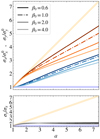 |
Fig. 8. Same as Fig. 6, this time for runs B3, A3, C3, and D3, that is, increasing β0. |
| In the text | |
|
Fig. 9. Root mean square amplitude of fluctuations for runs Y3h (no expansion, left panel) and Y3 (ɛ0 = 0.4, right panel). Magnetic (green) and velocity (red) fluctuations are normalised to the average sound speed (magnetic fluctuations are expressed in Alfvén units before normalisation, see text), while density fluctuations (light green, dash-dotted) are normalised to the average density. The average sound speed and the square of the current density are also plotted with purple and black dashed lines, respectively. In the right panel, the predicted a−2/3 decay for sound speed is drawn as a grey dotted line. |
| In the text | |
|
Fig. 10. Omnidirectional spectra of velocity and magnetic field (Eq. (19)) as a function of the normalised wave number for run Y3. Different times are shown as indicated in the colour bar. The spectrum corresponding to the flux rope is visible at k/k0≲6 in the magnetic spectrum. |
| In the text | |
|
Fig. 11. Snapshots for successive times of the magnetic field for run Y3. The total magnetic field |B| is represented by the colour-coded map, and the in-plane magnetic field is shown with constant-Az black lines. Only a portion of the domain is shown, see text. |
| In the text | |
|
Fig. 12. Maps of the in-plane magnetic field, |
| In the text | |
|
Fig. 13. Snapshot at t = 16.0 (a = 7.4) of the magnetic field for runs A3 (isolated flux rope), Z3 (with fluctuations smaller inside the flux rope by a factor 5), and Y3 (with equal fluctuation amplitude everywhere). The axial field Bz is represented by the colour-coded map, whereas the in-plane magnetic field is represented with constant-Az black lines. The two rows show the same fields (colour map and black iso-contours) but differ for the tracer, which is plotted with a thick white line: in the top row, we show the pinch tracer that is initially co-spatial with the in-plane (poloidal) magnetic field; in the bottom row, the white lines bound the axial tracer that is initialised in the same region occupied by the out-of-plane (axial) magnetic field. |
| In the text | |
|
Fig. 14. Heliospheric evolution of the pinch tracer sizes (σx and σy) for runs A3 (no turbulence, dash-dotted line), Z3 (turbulence out greater than in, dashed line), Y3 (turbulence in and out, dotted line), and Y3k (turbulence in and out at smaller scales, densely dash-dotted line). The light blue (orange) broad line represents the expected ‘kinematic’ trend along x (y). |
| In the text | |
|
Fig. 15. Heliospheric evolution of the flux rope radial size S[AU] versus distance R[AU] for runs A2-A6. Only the range a>2 (R>0.29 AU) is considered, to avoid the first dynamical transient for most runs (even though it is still visible and important in runs A4-A6). The estimates of S using σx are drawn as markers (different shapes for different runs), and each run has been fitted with a power law (solid lines with different colours). The solid thin black line is the linear (αR≡1) trend. The shaded grey area highlights the range between the minimum and maximum αR values obtained by randomly sampling data points from the combined set of runs A2-A6 (see text for details). |
| In the text | |
|
Fig. 16. Total magnetic field intensity |B| (top panel) and radial velocity ux (bottom panel) for runs A2-A6, along a radial cut through the flux rope axis, for the final times (R≃1 AU). In the bottom panel, the peak of ux is drawn with markers (the same as in Fig. 15 for each run) and labelled with the corresponding estimate of the non-dimensional expansion parameter ζ; the position corresponding to the peak is drawn as a light dashed vertical line in the top panels, to compare it to the magnetic boundaries. Run A3 is shown as a dash-dotted line in both panels. |
| In the text | |
Current usage metrics show cumulative count of Article Views (full-text article views including HTML views, PDF and ePub downloads, according to the available data) and Abstracts Views on Vision4Press platform.
Data correspond to usage on the plateform after 2015. The current usage metrics is available 48-96 hours after online publication and is updated daily on week days.
Initial download of the metrics may take a while.