| Issue |
A&A
Volume 699, July 2025
|
|
|---|---|---|
| Article Number | A159 | |
| Number of page(s) | 14 | |
| Section | Cosmology (including clusters of galaxies) | |
| DOI | https://doi.org/10.1051/0004-6361/202554502 | |
| Published online | 07 July 2025 | |
The ESPRESSO Redshift Drift Experiment⋆
I. High-resolution spectra of the Lyman-α forest of QSO J052915.80-435152.0
1
INAF – Osservatorio Astronomico di Trieste, Via G.B. Tiepolo, 11, I-34143 Trieste, Italy
2
Dipartimento di Fisica dell’Università di Trieste, Sezione di Astronomia, Via G.B. Tiepolo, 11, I-34143 Trieste, Italy
3
INFN – National Institute for Nuclear Physics, via Valerio 2, I-34127 Trieste, Italy
4
Centro de Astrofísica da Universidade do Porto, Rua das Estrelas, 4150-762 Porto, Portugal
5
Instituto de Astrof’ısica e Ciências do Espaço, Universidade do Porto, Rua das Estrelas, 4150-762 Porto, Portugal
6
Faculdade de Ciências, Universidade do Porto, Rua do Campo Alegre, 4150-007 Porto, Portugal
7
IFPU – Institute for Fundamental Physics of the Universe, via Beirut 2, I-34151 Trieste, Italy
8
Hamburger Sternwarte, Universitaet Hamburg, Gojenbergsweg 112, D-21029 Hamburg, Germany
9
European Southern Observatory (ESO), Karl-Schwarzschild-Str. 2, 85748 Garching bei Munchen, Germany
10
INAF – Arcetri Astrophysical Observatory, Largo E. Fermi 5, I-50125 Florence, Italy
11
Instituto de Astrofísica de Canarias (IAC), Calle Vía Láctea s/n, E-38205 La Laguna, Tenerife, Spain
12
Departamento de Astrofísica, Universidad de La Laguna (ULL), E-38206 La Laguna, Tenerife, Spain
13
Centre for Astrophysics and Supercomputing, Swinburne University of Technology, Hawthorn, Victoria 3122, Australia
14
Instituto de Astrofísica e Ciências do Espaço, Faculdade de Ciências da Universidade de Lisboa, Campo Grande, PT1749-016 Lisboa, Portugal
15
Departamento de Física da Faculdade de Ciências da Universidade de Lisboa, Edifício C8, 1749-016 Lisboa, Portugal
16
Observatoire Astronomique de l’Université de Genève, Chemin Pegasi 51, CH-1290 Versoix, Switzerland
17
Center for Space and Habitability, University of Bern, Gesellschaftsstrasse 6, Switzerland
18
Cerro Tololo Inter-American Observatory/NSF NOIRLab, Casilla 603, La Serena, Chile
19
INAF – Osservatorio Astronomico di Padova, Vicolo dell’Osservatorio 5, I-35122 Padova, Italy
20
INAF – Osservatorio Astrofisico di Torino, Via Osservatorio 20, I-10025 Pino Torinese, Italy
21
Centro de Astrobiología, CSIC-INTA, Camino Bajo del Castillo s/n, 28602 Villanueva de la Cañada, Madrid, Spain
⋆⋆ Corresponding author: This email address is being protected from spambots. You need JavaScript enabled to view it.
Received:
12
March
2025
Accepted:
27
May
2025
Abstract
Context. The measurement of the tiny temporal evolution in the redshift of distant objects, the redshift drift, is a powerful probe of universal expansion and cosmology.
Aims. We performed the first steps towards the measurement of such an effect using the Lyman-α forest in the spectra of bright quasars as a tracer of cosmological expansion. Our immediate goal is to determine to which precision a velocity shift measurement can be carried out with the signal-to-noise (S/N) level currently available and whether this precision aligns with previous theoretical expectations. A precise assessment of the achievable measurement precision is fundamental for estimating the time required to carry out the whole project. We also aim to study possible systematic effects of an astrophysical or instrumental nature arising in the measurement.
Methods. We acquired 12 hours of ESPRESSO observations distributed over 0.875 years of the brightest quasar known, J052915.80-435152.0 (zem = 3.962), to obtain high-resolution spectra of the Lyman-α forest, with a median S/N of ∼86 per 1 km s−1 pixel at the continuum. We divided the observations into two distinct epochs and analysed them using both a pixel-by-pixel method and a model-based approach. This comparison allows us to estimate the velocity shift between the epochs, as well as the velocity precision that can be achieved at this S/N. The model-based method is calibrated using high-resolution simulations of the intergalactic medium from the Sherwood Simulation Suite, and it provides greater accuracy compared to the pixel-by-pixel approach.
Results. We measure a velocity drift of the Lyman-α forest consistent with zero: Δv = −1.25−4.46+ 4.44 m s−1, equivalent to a cosmological drift of v˙ = −1.43−5.10+5.08 m s−1 or ż = −2.19−7.78+7.75 × 10⁻⁸ yr−1. The measurement uncertainties are on par with the expected precision. We estimate that reaching a 99% detection of the cosmic drift requires a monitoring campaign of 5400 hours of integration time over 54 years with an ELT and an ANDES-like high-resolution spectrograph.
Key words: instrumentation: spectrographs / quasars: absorption lines / cosmology: observations / quasars: individual: J052915.80-435152.0
Based on Guaranteed Time Observations collected at the European Southern Observatory under ESO programmes 110.247Q and 112.25K7 by the ESPRESSO Consortium.
© The Authors 2025
 Open Access article, published by EDP Sciences, under the terms of the Creative Commons Attribution License (https://creativecommons.org/licenses/by/4.0), which permits unrestricted use, distribution, and reproduction in any medium, provided the original work is properly cited.
This article is published in open access under the Subscribe to Open model. This email address is being protected from spambots. You need JavaScript enabled to view it. to support open access publication.
1. Introduction
Directly measuring the expansion history of the Universe is among the most pressing tasks of observational cosmology, especially considering the evidence of its recent acceleration phase (Riess et al. 1998, 2021; Garnavich et al. 1998; Albrecht et al. 2006; Dawson et al. 2013, 2016; Martins 2024; Adame et al. 2025). Most studies aiming to do this include specific assumptions on an underlying model, or class of models, leading to cosmological constraints that are model-dependent. A conceptual alternative, not yet realised in practice but expected to be achieved by forthcoming astrophysical facilities, is the redshift drift measurement, also known as the Sandage test.
As was first explored by Sandage (1962), the evolution of the Hubble expansion causes the redshift of distant objects participating in the Hubble flow to change slowly with time. Just as the cosmological redshift, z, provides evidence of the expansion, the drift in this redshift provides evidence of the expansion's acceleration or deceleration between the epoch z and the present one. This implies that the expansion history of the Universe can be detected and mapped, at least in principle, by means of a straightforward spectroscopic monitoring campaign.
For simplicity, we take a generic metric theory of gravity with the further assumption of homogeneity and isotropy, in which case the evolution of the metric tensor is entirely specified by the global scale factor, a(t). A photon emitted by some object at comoving distance, χ, at the time, tem, and observed by us at tobs, will have a redshift of
 (1)
(1)
Now consider how the redshift of an object at a fixed comoving distance, χ, evolves with tobs. Over a comparatively short timescale, Δtobs, it will drift by
 (2)
(2)
which, differentiating Eq. (1) with respect to tobs, leads to
![Mathematical equation: $$ \frac {dz_\chi }{dt_{\mathrm {obs}}}(t_{\mathrm {obs}}) = \left [1+z_{\chi }(t_{\mathrm {obs}})\right ]H(t_{\mathrm {obs}})-H(t_{\mathrm {em}}). $$](/articles/aa/full_html/2025/07/aa54502-25/aa54502-25-eq6.gif) (3)
(3)
Finally, we obtain, in a simplified form (McVittie 1962),
 (4)
(4)
Measuring ż for a number of objects at different z gives the function ȧ((z) and, given a(z), it is possible to reconstruct a(t). Therefore, a measurement of ż amounts to a purely dynamical and model-independent reconstruction of the expansion history of the Universe.
The effect is conceptually simple and provides a tool for key cosmological tests. Inter alia, one can easily verify that in decelerating universes, one expects a negative redshift drift at all redshifts. Conversely, a positive drift signal implies a violation of the strong energy condition, and hence the presence of some form of dark energy that accelerates the Universe (Liske et al. 2008; Uzan et al. 2008; Quercellini et al. 2012; Heinesen 2021). Mapping the redshift evolution of the drift can also lead to constraints on parameters in specific models, either alone or in combination with traditional cosmological probes (Alves et al. 2019; Rocha & Martins 2022; Marques et al. 2023, 2024).
The theoretical framework outlined above highlights the immense potential of redshift drift measurements to directly probe the expansion history of the Universe in a cosmological model-independent manner. However, achieving the sensitivity required to detect this effect is an observational challenge due to its exceedingly small expected magnitude. For instance, over a timescale of ∼10 years, the redshift drift, ż, in a Λ Cold Dark Matter cosmology (ΛCDM, Planck Collaboration VI 2020) is typically of the order of 10−10 to 10−9, or a few centimetres per second per decade in spectroscopic terms, for 0<z<6. Such precision necessitates both an adequate tracer population and a high-resolution spectroscopic capability that ensures the systematic uncertainties are smaller than the signal itself.
Among the possible tracers for this effect, the Lyman-α forest stands out as a particularly promising candidate (Loeb 1998). The Lyman-α forest consists of a series of absorption lines imprinted on the spectra of distant quasars due to intervening clouds of neutral hydrogen in the intergalactic medium (IGM). The suitability of the Lyman-α forest for redshift drift measurements arises from several key factors:
-
Low cosmic overdensities: The Lyman-α forest arises from sparse intergalactic neutral hydrogen, which is physically unconnected with the background source, faithfully tracing the Hubble flow, apart from seldom strong absorbers due to dense intervening galactic environments (Rauch 1998).
-
Abundance of tracers: The Lyman-α forest provides a dense sampling of absorption features along the line of sight (with number density dn/dz≈100−200 at z = 2−3, Kim et al. 2002), enabling the measurement of the redshift drift across numerous independent systems at varying redshifts.
-
Spectroscopic accessibility: Even though the Lyman-α lines are not particularly narrow, with a typical linewidth of ∼30 km s−1 (Kim et al. 2002), through the use of high-resolution spectroscopy their positions can be determined with sufficiently high precision to enable the measurement of the redshift drift. Moreover, the Lyman-α lines at z>1.5 are observable with large ground facilities.
-
High-redshift sensitivity: At high redshifts, specifically deep in the matter era where the Universe is decelerating, the term (1+z) in Eq. (4) amplifies the magnitude of the drift, making the signal more detectable (see Fig. 2 in Liske et al. 2008).
Thus far, no detection of this signal is available, and existing upper limits based on other probes such as H I 21cm absorption lines (Darling 2012) and narrow metal absorption lines (Cooke 2020), have error bars three orders of magnitude larger than the expected signal. The first detections of the signal are expected to come from the ArmazoNes high Dispersion Echelle Spectrograph (ANDES) at the ESO's Extremely Large Telescope (ELT) (Marconi et al. 2024; Martins 2024) and by the full configuration of the Square Kilometre Array (SKA) (Klöckner et al. 2015; Kang et al. 2025), which are sensitive to the high redshift (matter era) and low redshift (acceleration era), respectively.
The Echelle SPectrograph for Rocky Exoplanets and Stable Spectroscopic Observations (ESPRESSO) spectrograph at the combined Coudé focus of ESO's VLT (Pepe et al. 2021) has a similar design to ANDES and enables us to bridge the gap between the present and the future. As part of the ESPRESSO Science Team's guaranteed time observations (GTO), we are carrying out the first dedicated redshift drift experiment, with a nominal experiment time of one year and an observation time of four nights (ca. 40 hours). This paper presents the first results, derived from 12h of observations of one quasar target.
Our two overarching goals are to improve the aforementioned upper limits and to start developing, testing, and validating a full end-to-end analysis pipeline, which will provide a baseline for the corresponding pipeline for the ANDES redshift drift measurement. This is the first of a series of reports on this experiment.
Specifically, in this work we set the first two epochs of observations with high-resolution, high-stability ESPRESSO spectroscopy and estimate the achievable precision. We check whether this aligns with previous estimates and if systematic effects of astrophysical or instrumental nature appear at the present level of signal-to-noise (S/N). We extrapolate our estimates to a realistic ANDES observational campaign to estimate the amount of time required to achieve a significant detection of the cosmological expansion.
In Sect. 2 we present the quasar targeted for our study. In Sect. 3 we describe the observation taken with ESPRESSO, the data reduction, the definition of the two observational epochs, and the recognition of metal lines and strong absorbers throughout the spectrum. The expected precision of a velocity drift measurement at the current level of S/N is presented in Sect. 4. In Sect. 5 we apply a direct pixel-by-pixel method, based on the work of Bouchy et al. (2001), to estimate the velocity shift, Δv, that has occurred between the two epochs. A different method of performing the measurement, based on modelling the Lyman-α forest, is presented in Sect. 6. In Sect. 7 we investigate the validity of our estimates and tackle the possible systematic effects arising in the measurement due to astrophysical or instrumental effects. In Sect. 8 we extrapolate our results to estimate the total observational time required to carry out a significant detection of the cosmological drift, either with ESPRESSO or with ANDES. Finally, we summarise and discuss our results in Sect. 9.
2. Target selection
The QUBRICS (QUasars as BRIght beacons for Cosmology in the Southern hemisphere) survey (Cristiani et al. 2023) provides a golden sample of seven bright quasars specifically selected to carry out the measurement of the redshift drift, observing their Lyman-α forest with an ESPRESSO- or ANDES-like spectrograph. For the present case study and the first epoch observation, we consider the brightest object from the golden sample, J052915.80-435152.0, hereafter called Super Bright 2 (SB2). In a parallel paper (Marques et al. in prep.) we shall discuss the observation of the second-most luminous object of the sample J212540.97-171951.4 (hereafter called SB1)1. SB2 has the identifier QID 1128023 in the QUBRICS database (Calderone et al. 2019) with coordinates (J2000) RA 05:29:15.81 and Dec −43:51:52.1 and magnitudes r = 16.3005, i = 16.1184 (Onken et al. 2024) and G = 16.3452 (Gaia Collaboration 2021).
Besides being particularly suited for the Sandage test, SB2 is an outstanding object, the most luminous quasar known in the Universe. Medium resolution spectra taken with X-Shooter (Vernet et al. 2011) reveal that SB2 has a bolometric luminosity of log(Lbol/erg s−1) = 48.27, supported by an accretion of 370 M⊙ per year onto a supermassive black hole (SMBH) of mass log M/M⊙∼10.24 or, in other terms, about one solar mass per day accreting onto a SMBH of ∼17 billion solar masses. From the same data, Wolf et al. (2024) report an emission redshift for SB2 of zem = 3.962.
3. Data acquisition and treatment
In this work, we present high-resolution, high-S/N optical spectroscopy of this outstanding object obtained with ESPRESSO. ESPRESSO observations have been carried out using the single UT mode (Pepe et al. 2021) and achieve a resolving power of R=λ/Δλ∼135 000, where Δλ is the full width at half maximum of resolution element (∼2.2 km s−1 in velocity space), with a 4x2 detector binning, chosen to optimise the S/N in the region covering the Lyman-α forest. A summary of the observations is given in Table 1.
Summary of single observing blocks (OBs) of SB2 taken during observing periods P110 and P112.
The observations were reduced using the ESPRESSO Data Reduction Software2 (DRS, Di Marcantonio et al. 2018), version 3.1.0. Laser Frequency Combs (LFC) frames were used for wavelength calibration of the spectra. We also produced spectra calibrated on the Fabry-Pérot (FP) etalon combined with a ThAr lamp frames to investigate the presence of possible instrumental systematics due to calibration stability and accuracy (see Sect. 7.5).
The final products of the pipeline were flat-fielded, blaze-corrected, sky-subtracted, and wavelength-calibrated. The spectra were also corrected to the Solar System barycentre using standard pipeline procedures, employing INPOP13c ephemeris (Fienga et al. 2014). Earth's precession is taken into account in the correction, consistently with the requirements for achieving sub-meter-per-second precision (Wright & Eastman 2014).
Order-by-order spectra were optimally extracted along detector rows (in the cross-dispersion direction), retaining for each pixel the original calibrated wavelength of the rows themselves, while the order-merged spectra were rebinned to a common wavelength grid.
The coaddition of the extracted spectra was performed using the ASTROCOOK software3 (Cupani et al. 2020), following the ‘drizzling’-like approach described in Cupani et al. (2016). A wavelength grid was defined with a fixed step of 1 km s−1, and the pixels contributing to each bin in the grid were selected from the order-by-order spectra, to combine them all together in a single rebinning procedure. Contributing pixels were weighted by their associated error and by how much they overlapped with the wavelength range of the bins themselves. Order-by-order spectra were equalised prior to coaddition by multiplying their flux by scalars to get the same median flux level, to eliminate differences in flux levels due to varying observing conditions.
Coaddition of individual exposures resulted in a single spectrum, with a median S/N ∼ 86 per 1 km s−1 pixel at the continuum level in the forest, and ∼105 redwards of the Lyman-α emission, as shown in Fig. 1. The Lyman-α forest highlighted in the figure is defined as the spectral interval between the Lyman-α and Lyman-β emission of the quasar, namely 509−603 μm, shown in more detail in Fig. 2. This section of the spectrum contains Lyman-α absorption lines with 3.18≤z≤3.96, and no Lyman-β absorptions.
 |
Fig. 1. Combined spectrum of SB2. Top panel: Flux density in arbitrary units is shown in black, with the dashed purple line denoting the flux density error. Bottom panel: S/N per 1 km s−1 pixel. The shaded green area highlights the Lyman-α forest considered in the redshift drift measurement, bound by the Lyman-α and Lyman-β emissions of the quasar, namely between 509−603 m. |
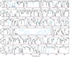 |
Fig. 2. Normalised transmitted flux of the Lyman-α forest in the combined spectrum of SB2 as a function of wavelength. The solid light blue line highlights the spectral regions masked due to metal absorption, the sub-DLA and bad pixels. The solid purple line reports the flux error. |
Observations taken in the two ESO observing periods P110 and P112 (see Table 1), respectively, were also combined separately to provide two independent spectra that were used as the two epochs of the Sandage test. The first (P110) and second (P112) epoch spectra have a median S/N level at the continuum in the Lyman-α forest of ∼47 and ∼72, respectively. We defined the temporal baseline occurring between the two epochs’ spectra as the difference between the mean observational date of each period Δt = 0.875 yr.
3.1. Removing metal transitions from the Lyman-α forest
As has been shown by Cristiani et al. (2024), Lyman-α and metal lines have significantly different dynamical behaviours on the temporal and physical scales probed by the experiment. The authors show that absorption lines due to neutral hydrogen on adjacent sightlines (with sub-kiloparsec separations) appear identical within the noise, whereas metal lines show significant differences in their velocity structure. These intrinsic dynamical effects can be a source of strong systematic effects, inducing a velocity shift in the metal lines up to a few centimetres per second per year, of the same order of magnitude as the expected cosmic signal. We therefore removed the metal-polluted regions from our analysis to reduce possible systematics.
This process was done using the ASTROCOOK software (Cupani et al. 2020) to provide a secure identification of metal lines in the spectrum. First, the quasar continuum emission was estimated by applying an iterative sigma-clipping procedure to remove absorption features while masking sky emission lines, telluric absorption lines, or spurious, narrow spikes in flux (e.g. ‘cosmic rays’ that were not removed by the coadding process), and manually correcting the continuum level where necessary. Sky and telluric lines were masked using a reference SKYCORR model (Noll et al. 2014) and empirically defining proper cuts to conservatively remove even the line wings. We performed a search for metal absorption lines throughout the spectrum, starting from line doublets (e.g. C IV, Si IV and Mg II) redwards of the Lyman-α emission and following up with associated lines, i.e. other ionic transitions at the same redshift as the found doublets. Table 2 reports the absorption systems, i.e. the groups of ionic transitions with the same redshift, found along the spectrum of SB2.
Metallic absorption systems identified in the spectrum of SB2.
Once identified, we fitted composite Voigt profiles to the metal absorption lines that fall redwards of the Lyman-α emission, estimating the absorber's redshift, column density, and Doppler broadening. Metal lines bluewards of the Lyman-α emission were not fitted, as this would require modelling multiple blended H I components, making the analysis significantly more complex. Since this is beyond the scope of the present study, we left it unaddressed and masked out such lines, removing the spectral regions in velocity space associated with higher wavelength transitions. A table reporting the fitted Voigt parameters for the metal transitions found redwards of the Lyman-α emission can be found in an electronic form at the CDS.
3.2. A sub-DLA at zabs = 3.63
As is visible in Fig. 1, the spectrum of SB2 presents a strong H I absorption at λ∼563 μm or z∼3.63. We study this absorbing system in more detail to understand, based on its column density, whether it might belong to a dense environment prone to proper motions related to galactic dynamical processes, or it stems from the sparse cosmic web following the Hubble flow and thus can be considered in the redshift drift measurement. We found strong and complex associated metal absorption redwards of the Lyman-α emission, stemming from ions with both low (O I, Al II, C II, Fe II, Si II) and high (C IV, Si IV) ionisation states. We fitted the Lyman-α absorber within Astrocook using 3 components, tying the redshifts of H I and low ionisation species. The total H I column density of the system is log NH I≈19.8, corresponding to a sub-Damped Lyman-α System (sub-DLA, Péroux et al. 2003).
Given this value, we decided to exclude the spectral range tied to this absorber from the analysis, as it is probably related to an intervening galactic system and could potentially induce systematics in the measurement due to its peculiar motions. We thus mask the region of the spectrum spanning ±2000 km s−1 from the column density weighted average redshift position of the system. The final masked spectra used in our analysis have 41 737 pixels (1 km s−1 wide) in the Lyman-α forest, compared to 50 805 pixels without mask. Meaning we consider only 82.15% of the total Lyman-α forest. Figure 2 shows the normalised flux of the Lyman-α forest in the spectrum of SB2, highlighting the masked-out regions.
4. Expected velocity precision
In a ΛCDM Universe (Planck Collaboration VI 2020), the expected cosmological redshift drift at redshift z = 3.573 (i.e. the middle of SB2's Lyman-α forest) is ż = −6.5 × 10⁻¹¹ yr−1, equivalent to  in velocity space. On the baseline of our experiment, the expected velocity shift between the two epoch spectra is therefore Δv=−0.38 cm s−1.
Liske et al. (2008) provided a practical formula to assess the precision expected from an experiment performed on the ELT based on an ensemble of quasars at different redshifts. We adapted this formula to estimate the precision expected from our data. Given the SB2 ESPRESSO spectra at the two epochs, we estimated the predicted precision in the velocity shift measurement, adapting the scaling relation of Liske et al. (2008)
 (5)
(5)
where S/N = 86 is the median S/N at the continuum level per 1 km s−1 pixel per object, accumulated over all observations (i.e. the S/N level of the combined spectrum). NQSO is the number of quasars in the sample (NQSO = 1 in our case), and zQSO = 3.962 is the redshift of the quasar. The γ exponent is 1.7 for zQSO≤4 and 0.9 above. The factor  is the fraction of the Lyman-α forest considered after masking. The factor g, called the ‘form factor’, depends on the observing strategy, being 1 if half of the exposures are taken at the beginning of the experiment and half at the end, and becoming larger if the measurements are spread out over time, reaching 1.7 for a uniform distribution (see Sect. 6 of Liske et al. 2008 for further details on the computation of the form factor). In our case, given the fact that 38% of the total integration time is collected at the first epoch, and 62% at the second, the form factor has a value of g = 1.03. From Eq. (5), we can estimate the expected maximum precision allowed by photon noise on our current data to be σv = 4.02 m s−1.
Note that in this work we have analysed only one sightline, whereas the relation from which Eq. (5) is derived has been calibrated on a measurement based on an ensemble of spectra. Sightline-to-sightline deviations from the predicted measurement precision due to cosmic variance are expected due to the varying number of Lyman-α lines and strong absorbers found in the spectra of different objects.
5. Redshift drift measurement: Pixel-by-pixel method
We first measured Δv using a method developed for measuring radial velocity shifts between repeated observations of stars for exoplanet search (Bouchy et al. 2001), which we refer to as the pixel-by-pixel method. In summary, due to the drift of the absorption lines, the flux of the i-th pixel at the second epoch, F2,i, can be expressed as a small perturbation of the flux in the same pixel at the first epoch, F1,i:
 (6)
(6)
where λi is the observed wavelength of the i-th pixel, and dFi/dλ is the slope of the spectrum at that pixel. The perturbation of the fluxes between two epochs defines, for each pixel, a small velocity shift, δvi. Note that Eq. (6) holds only for δvi much smaller than the typical line width (∼30 km s−1). The single pixel's velocities can be averaged over the whole spectrum to estimate the velocity drift occurring between the two epochs.
 (7)
(7)
where each pixel is weighted by  , i.e. the inverse variance of δvi. Accounting for the uncertainties in both epochs’ spectra and in their derivative, the variance becomes
![Mathematical equation: $$ \sigma ^2_{v_i} = \left [\frac {c}{\lambda _i (dF_i/d\lambda )}\right ]^2\left [\sigma _{1,i}^2+\sigma _{2,i}^2+ \frac {(F_{2,i} - F_{1,i})^2}{(dF_{i}/d\lambda )^2}\sigma ^2_{F'_i}\right ], $$](/articles/aa/full_html/2025/07/aa54502-25/aa54502-25-eq14.gif) (8)
(8)
where σ1,i and σ2,i are the i-th pixel flux error in the two spectra, and  is the error on the flux slope at the i-th pixel. With this choice of weights, the uncertainty on the final Δv estimate is
![Mathematical equation: $$ \sigma _v = \left [\sum _i \sigma ^{-2}_{v_i}\right ]^{-1/2}. $$](/articles/aa/full_html/2025/07/aa54502-25/aa54502-25-eq16.gif) (9)
(9)
It is worth noting that, at first order, the flux slope term dFi/dλ is epoch-invariant (under the assumption of very small shifts) and does not carry any epoch-dependent information. For this reason, we computed the flux derivative by means of finite differences of non-adjacent points, on the second epoch spectrum to exploit the higher S/N level and lower the noise in its evaluation.
We evaluated the velocity shift, δv, occurring between the two epochs, exploiting the normalised fluxes in the Lyman-α forest of the two spectra, where we have masked metal lines, the strong H I absorber at z∼3.63, and bad pixels. Our estimate yields Δv=−2.67±6.64 m s−1. Taking into account the mean baseline between the two epochs of Δt = 0.875 years, we estimate a drift of  , equivalent to a redshift drift of ż = (−0.47 ± 1.15) × 10−7 yr−1.
6. Redshift drift measurement: Model-based
The larger than expected uncertainty from the direct method is surprising and is not completely understood whether it stems from either instrumental systematics or problems in the measurement procedure, or whether it is intrinsic to our sightline. Loss of precision prolongs the time required for reliably detecting the redshift drift signal and raises the risk of critical failure. A secure estimate of the measurement uncertainty is therefore of crucial impact on the experiment timeline.
In this section, we develop a different approach to the measurement to investigate whether a higher precision can be achieved with the current data. Instead of directly comparing the two epochs’ spectra, we built an ensemble of analytical models of the forest of SB2 that are then correlated to the two epochs. The modelling procedure is calibrated on mock spectra extracted from state-of-the-art physical simulations of the IGM and is thus ‘informed’ on the spectral scales of the single Lyman-α lines and is able to de-prioritise pixels that might be affected by metal transitions or outlier pixels (e.g. non-removed cosmic rays). With this approach, we are capable of reducing the uncertainty in the measurement by a significant fraction and decreasing the total amount of integration time needed for the experiment.
Summarising, the main steps of the method are:
-
Production of realistic mock sightlines that reproduce the properties of the ESPRESSO spectra of SB2 considered in the measurement.
-
Calibration of the modelling procedure on the mock data.
-
Construction of an ensemble of models of the Lyman-α forest of SB2.
-
Evaluation of the velocity shift between the model ensemble and the first and second epoch data.
We stress that the mock data were only used to calibrate the modelling procedure and were not involved in the final measurement.
6.1. Mock spectra
We used realistic mock spectra that reproduce the properties of the three SB2 spectra (first epoch, second epoch, and combined) to calibrate the modelling pipeline and validate the measurement results. Starting from the hydrodynamical cosmological simulations of the IGM of the Sherwood Simulation Suite (Bolton et al. 2017) (with a box size of 10 Mpc/h and 2×10243 dark matter and gas particles), we extracted the gas particle data and computed the H I optical depth along 5000 skewers piercing the box at every redshift step Δz = 0.1, within 3.1≤z≤4. The optical depth of the spectra was rescaled to match the mean optical depth observed at z∼3.57 (centre of the forest) from Becker & Bolton (2013). The sightlines (10 Mpc/h long) are randomly selected from the appropriate redshift interval, shifted so that they begin and end with regions of no absorption, and stitched together to form 100 spectra that match the length of the Lyman-α of SB2 (∼421 Mpc/h long, or 50 321 km s−1).
The long spectra were then convolved with a Gaussian of FWHM ∼2.2 km s−1 to mimic ESPRESSO's resolution and re-binned to a grid of pixels 1 km s−1 wide (the average native pixel size extracted from the simulation was 0.593 km s−1), matching the binning of our data. The noise properties of the original spectrum were added to the mocks following the prescription of Rorai et al. (2017) (see also Trost et al. 2025). Summarising, the original first epoch spectrum was divided into ten chunks, ∼10 nm wide. For each of these chunks, we:
-
divided the pixels into 50 bins according to their normalised flux value, producing 50 corresponding noise distributions;
-
assigned a noise value to each simulated pixel, where the value was randomly sampled from the distribution associated with the pixel's flux value, as defined in the point above.
This procedure was repeated for each chunk of the first epoch spectrum and its corresponding mock spectra, to preserve the relation between S/N at the continuum level and wavelength.
The second epoch spectra were generated in the same way from the same sightlines. However, before sightline extraction, we artificially added a velocity drift of −0.38 cm s−1, i.e. the expected drift at z∼3.57 for a ΛCDM Universe during our baseline Δt = 0.875 yr, to the simulated particles’ velocities. These sightlines were then processed in the same way, and the noise of the second epoch was added to the flux, as explained above.
We combined the first and second epochs’ mock datasets via a weighted average, with weights proportional to the inverse of the pixels’ flux variance, to create the mock combined spectrum. Figure 3 shows the distribution of the S/N per pixel in the three mock datasets and the original spectra. To further validate the analysis (see Sect. 7), we also built second epoch mock datasets assuming either no drift between the two epochs or 103 and 104 years of temporal separation, adding a velocity drift to the simulation's particles of −3.8 m s−1 and −37.6 m s−1, respectively. On all spectra, we applied the same pixel masking of the original data, derived from metal, sub-DLA and bad pixels’ removal, to ensure the absence of systematics in the final measurement due to pixel masking and to conserve the total amount of pixels involved in the measurement.
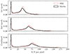 |
Fig. 3. Distribution of the S/N per pixel in the Lyman-α forest of the three spectra of SB2 (dashed red) and of the corresponding mock spectra (solid black). Upper panel: First epoch. Middle panel: Second epoch. Bottom panel: Combined spectrum. |
6.2. Model assessment
We relied on mock data to calibrate the modelling procedure before building the best possible model of SB2. Multiple sightlines were considered in the calibration to properly account for cosmic variance effects in the modelling procedure. Given the short timescales between the two epochs and that the total S/N is insufficient to detect the cosmic drift signal, we simplified the procedure by creating a fiducial model of the combined spectrum instead of modelling the two epoch spectra individually. A further simplification regards our decision to model the spectrum using cubic splines4 instead of the more traditional approach using Voigt profile decomposition. This was done because we were not interested in measuring physical properties of the gas but rather differences between the SB2's spectra in the two epochs, for which the spline method was sufficient.
In quasar spectra, Lyman-α lines have a typical width of ∼30 km s−1 (Kim et al. 2002), while outlier features (e.g. cosmic rays) and metal transitions are typically narrower (down to a few kilometres per second). We calibrated the spline knot spacing on mock spectra containing only Lyman-α absorption, so that our procedure was ‘informed’ on the scales that we want to probe. Then, by generating an ensemble of models for SB2, we recovered a higher variance among models in the regions that might be affected by sharp non-Lyman-α absorption and could de-prioritise such features in the final measurement of Δv. The described procedure also prevents over-fitting of the noise.
In practice, let Sk(λ|n(A,ϕ)) be the spline model fitted on the k-th spectrum of the combined mock dataset described in the previous section, using the square inverse of the flux noise as weights in the fit, where n is a vector defining the positions of the spline knots along the spectrum. The knots are equispaced in velocity space, separated by a constant velocity, A, starting from an initial position (or phase) 0<ϕ<A with respect to the beginning of the Lyman-α forest.
Goodness of fit for the model was determined from its residuals to the data,  . We considered a model to be good if the residuals are centred at zero with a variance equal to unity,
  .
.
One hundred mock spectra were fitted in this way, varying both the inter-nodal distance A and the initial phase ϕ, and their residuals were calculated as above. For each value of A and ϕ, we calculated the mean and the variance of the residuals for all 100 mock spectra. The optimal value of A was determined by examining which combination of parameters results in residuals most closely matching values drawn from  . Mathematically, we searched for a value of A that minimises:
 (10)
(10)
where σR(A) is the standard deviation of the fit residuals of splines with internodal distance A, averaged over all spectra and all considered initial node phases.  is the variance of the quantity σR(A) due to sightline variance and variations in the initial node phase. Figure 4 shows σR−1 and its variance as a function of internodal distance A. Minimising Eq. (10) yields a best inter-nodal distance of
  . Note that this value of A is valid only for this precise S/N level, resolution, pixel size, and redshift. For any change in the spectral properties, A should be re-evaluated.
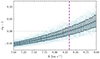 |
Fig. 4. Standard deviation of the fit residuals between the combined mock spectra's flux and the spline model with internodal distance A. The blue squares describe the σR of models on different mock spectra and randomly drawn initial node phase ϕ. The black error bars define the average and standard deviation of σR(A)−1. The vertical dashed purple line denotes the optimal value of A. |
6.3. Building the forest model
Given the optimal knot spacing and its uncertainty, A and σA, we were able to construct a large number of models of the Lyman-α forest of SB2 that describe the data equally well in terms of a goodness-of-fit statistic (e.g. χ2). This allowed us to more thoroughly assess the impact of model non-uniqueness on the final result. This is conceptually similar to the approach taken by, for example, Lee et al. (2021), Milaković et al. (2024), Webb et al. (2025) in the context of fundamental constant and isotopic ratio measurements. Additionally, we identified parts of the spectrum where model non-uniqueness was minimal so that those regions could be prioritised in our analysis, whereas regions where model diversity (and hence uncertainty) was larger are considered ‘less trustworthy’. Moreover, we implemented a weighting scheme based on the model's gradient and its uncertainty, mimicking the pixel-by-pixel method (Sect. 5), to achieve a larger sensitivity to velocity shifts. Both aspects are major benefits of the model-based method, which results in a better handling of uncertainties.
We started by fitting the combined SB2 spectrum with N = 500 splines, Sj(λ | nj). The node positions of the j-th model, nj, were generated starting from an equispaced sequence of nodes in velocity space, nj,0, with inter-nodal separation, Aj, drawn from a normal distribution,  , and initial phase 0≤ϕj<Aj, drawn with uniform probability. The node positions were then perturbed by adding random noise in velocity space as nj=nj,0+m, where each element of the m array was randomly drawn from a normal distribution,
  .
.
From the ensemble of spline models, we evaluated the mean model,  , and the variance between the models,
  .
.
Figure 5 shows a region of the first, second, and combined spectra, alongside the mean spline model. In the figure, flux noise and model variance are shown in the middle panel. The periodic pattern found in the flux noise results from the coaddition of several exposures and the subsequent rebinning to a fixed grid, which creates an aliasing effect in the error arrays, whose frequency depends on the position of the pixels within the spectral order. The bottom panel shows the pixel weights used in the measurement (see Eq. (12)), proportional to the local model derivative.
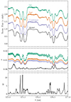 |
Fig. 5. Section of the SB2 spectrum. Top panel: Normalised flux of the first epoch (green), second epoch (orange), and combined (purple) spectra. The mean model, |


6.4. Velocity drift estimate
Strictly speaking, |ż| is larger at the red end of the Lyman-α forest than at its blue end, causing a redshift dependent compression of features in our spectrum. However, this effect is tiny and completely negligible at the S/N of our data. We therefore ignored the redshift dependence of ż and assumed that only a rigid translation Δv, in velocity space, occurred between the two epochs. Δv was measured indirectly, by first calculating the velocity shifts δv occurring between individual epochs and the model. The measured shift between two epochs is then: Δv=δv2−δv1, where subscripts identify the epoch.
The value of δv was obtained through a Monte Carlo Markov chain (MCMC) process with a modified Gaussian likelihood of the form:
 (11)
(11)
where the sum was performed over all non-masked pixels. F and σF are the normalised flux and its uncertainty, respectively, of either the first or second epoch spectra of SB2. Npix is the number of non-masked pixels,  is the mean spline model, and
  is the variance within the ensemble of spline models, where the latter is included as an additional term at the denominator to effectively consider the pixels for which the ensemble's models are not consistent as less trustworthy. For both terms, the dependence on δv denotes the fact that the splines’ nodes have been solidly shifted by δv in velocity space, and the models are re-evaluated on the spectrum's pixel grid at each step of the MCMC process. The term W contains information on pixel weights.
Similarly to Bouchy et al. (2001), we wanted to assign a higher weight to pixels sensitive to velocity shifts, such as those with large flux gradients (i.e. the sides of the lines) and those for which variance in the flux gradient is minimal (i.e. for which models are consistent). The former aspect is similar to what is done in Sect. 5, but the latter aspect was only possible because we produced a large number of spline models. The two contributions were defined by evaluating the mean derivative (in absolute values)  and the standard deviation within first derivatives’ magnitudes in the model ensemble σS′. The weights were therefore defined as
![Mathematical equation: $$ W(\lambda _i|\delta v) = N_{pix}\frac {\bar {S}'(\lambda _i|\delta v)}{\sigma _{S'}(\lambda _i|\delta v)} \left [\sum _j^{N_{pix}} \frac {\bar {S}'(\lambda _j|\delta v)}{\sigma _{S'}(\lambda _j|\delta v)}\right ]^{-1}, $$](/articles/aa/full_html/2025/07/aa54502-25/aa54502-25-eq34.gif) (12)
(12)
where  and σS′ are the mean absolute model derivative and its standard deviation among models. The normalisation of the W term is assumed such that
 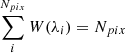 , as in the non-weighted case (W(λi) = 1 for all pixels). As
  and
and  , W is also recalculated at each step of the MCMC process. In practice, the new scheme resulted in weighting line edges more strongly than the continuum and other flat regions, as seen in the bottom panel of Fig. 5.
We ran MCMC to estimate δv for each epoch independently. Figure 6 shows the posterior probability distributions probed by the MCMC analysis for δv1 (filled green) and δv2 (orange). The obtained results for the shifts are 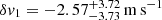 and
and 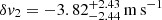 , where the uncertainties correspond to the 16th and 84th percentiles of the posterior distribution and should be considered equivalent to the 68% confidence interval. Taking the difference between the two values above and propagating their uncertainties, we obtained a velocity shift between the two epochs of
 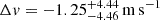 , which translates into a drift of
  or
or 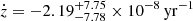 .
.
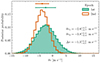 |
Fig. 6. Posterior probability distributions obtained by the MCMC analysis comparing the mean model to the spectra of epoch 1 (filled green) and epoch 2 (orange) through the likelihood defined in Eq. (11) (see Sect. 6.4). Scatter points with error bars define the median values and the 68% confidence intervals. |
Both estimates of δvi have negative values. While this may first seem surprising, there is an easily understandable explanation related to the weighting scheme implemented in Eq. (11). To demonstrate this, we carried out a simple test of measuring δv on the combined spectrum, i.e. the same spectrum used to produce our 500 models. Naïvely, this should return a shift consistent with zero. Applying our measurement method to this data resulted in 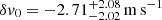 , a value that is negative and marginally inconsistent with zero. However, temporarily fixing W = 1 in Eq. (11) resulted in
 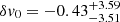 , consistent with zero. Obviously, our choice of W has given more weight to pixels with negative contributions to δv while simultaneously decreasing measuring uncertainties. Another way of looking at this is through a comparison of δv0 with δv1 and δv2. Comparing their values, one sees that δv0 falls in between δv1 and δv2, as expected. In that sense, the obtained values of δv1 and δv2 are not surprising.
7. Validation and systematics
7.1. Measurement validation
We validated the measurement procedures by applying the pixel-by-pixel (see Sect. 5) and the model-based (see Sect. 6.4) methods to a synthetic sample of mock spectra for which we know a priori the velocity shift occurring between the two epochs. We thus produced mock datasets assuming the same S/N distribution, pixel size, spectral range, and resolution of the SB2 spectra, simulating a Δv of 0 cm s−1, −0.38 cm s−1, −4.3 m s−1, and −42.9 m s−1, corresponding to a temporal baseline of zero, 0.875, 103 and 104 years in a ΛCDM Universe.
We applied our methods to ten random sightlines from each mock dataset, with the results shown in Fig. 7. The top panel shows the measured velocity shifts, Δv, obtained with the pixel-by-pixel (blue) and model-based (red) methods in the four baseline cases. Both methods were applied to the same set of 10 sightlines. We found that the two methods are capable of recovering the imposed drift, with an uncertainty that depends solely on the S/N level of the two spectra (matched to the SB2 data, regardless of the simulated Δv) and on the number of Lyman-α lines contained in each sightline. The scatter among the ten measured velocity shifts is consistent with the estimated uncertainties. Notably, the pixel-by-pixel method shows a slight discrepancy between the expected signal and the mean measured Δv when applied to the longest baseline of 10 000 years. The cause of such bias is not clear, although it could stem from the perturbative assumption taken in Eq. (6) that might not hold any longer for the large shift imposed in this simulated case. Nonetheless, our aim is to measure very small shifts for which such an assumption is solid. The model-based method recovers the imposed shift well in all instances.
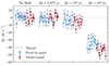 |
Fig. 7. Velocity shift, Δv, measured on ten random mock sightline pairs with both the pixel-by-pixel (blue square scatter points, see Sect. 5) and model-based methods (red diamond scatter points, see Sect. 6.4) where a different baseline is assumed between the two epochs. The horizontal blue dotted and dashed red lines report the average Δv measured with the pixel-by-pixel and the model-based methods, respectively. From left to right, the mock datasets are built assuming no shift (Δvexp = 0 m s−1), Δt = 0.875 yr (the same time elapsed between the two observed spectra, Δvexp=−0.38 cm s−1), Δt = 103 yr (Δvexp=−4.3 m s−1), and Δt = 104 yr (Δvexp=−42.9 m s−1). The dashed grey lines report the assumed shift. |
7.2. Uncertainty across the spectrum
It is possible that a narrow segment of the Lyman-α forest contains unidentified contaminants that spoil the measurement on Δv. We investigated this possibility by dividing the Lyman-α forest into ten equally sized chunks (of width 9.4 nm) and measuring Δv over each individual one, using both the pixel-by-pixel and model-based methods, following the usual procedures described in Sects. 5 and 6.4.
Figure 8 shows the measured Δv for each chunk, as a function of the chunk's central wavelength λc, in the upper panel. The middle panel shows the velocity shift uncertainty, σv, computed on each chunk with the pixel-by-pixel (blue) and model-based (red) methods. In the absence of systematics, the measurement uncertainty is expected to depend solely on the median S/N at continuum and the number of pixels (or the fraction of the forest  ) in each chunk, scaling as
  . The expected measurement uncertainty is shown in the middle panel as a dash-dotted (dashed) grey line, scaled by the pixel-by-pixel (model-based) uncertainty obtained on the full spectrum. The estimated uncertainties closely follow the scaling expectations for both methods, highlighting the absence of wavelength-dependent systematic effects.
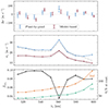 |
Fig. 8. Estimated velocity shift, Δv, computed on ten equispaced sections of the Lyman-α forest. Top panel: Δv estimated on each spectral chunk with the pixel-by-pixel (blue squares) and model-based (red diamonds) methods, as a function of the section's central wavelength λc. Middle panel: Measurement uncertainty, σv, for the two methods, shown with the same colour coding as the panel above. The dash-dotted and dashed grey lines report the expected uncertainty of the two methods, based on the median S/N and pixel number of each chunk. Bottom panel: Fraction of the Lyman-α forest |

7.3. Influence of the quasar
Given the extraordinary nature of SB2 (Wolf et al. 2024), with its high black hole accretion rate (Ṁ ∼ 370 M⊙ yr−1) and luminosity variability (∼15% over the last 6 years), one would expect to find a strong signature of IGM photoionisation in the Lyman-α forest close to the quasar emission redshift. However, our data do not show an important decrease in strength and number of Lyman-α lines close to zem, nor a significant variability of such lines, which could be related to the quasar's strong activity. Therefore, in our previous analysis, we based the redshift drift measurement on the whole forest, without excluding the proximity region, about 5000 km s−1 from the quasar emission redshift.
We checked for systematic effects due to the proximity to the quasar by performing the same measurement as before, but excluding such a region, and measured a velocity drift between the two epochs of Δv = 3.88±5.08 m s−1. Having excluded the proximity region reduces the number of pixels used in the measurement to ∼37 400, or ∼74% of the total amount found in the forest. When ignoring the proximity region, we excluded the range close to the Lyman-α emission where the spectra have the highest S/N levels at the continuum, with a median of 89, 134 and 161 per pixel in the first epoch, second epoch, and combined spectra, respectively, and performed the measurement on spectra with effectively lower S/N. Therefore, the uncertainty grows not only due to a reduced pixel sample, but also due to a smaller median S/N level (∼82 per pixel at the continuum in the combined spectrum) outside of the proximity region. These two effects add up to a scaling factor  , explaining the new uncertainty. Still, the measurement is compatible with the expected value, and no systematic effect due to excluding or taking into account the proximity region is clearly visible.
7.4. Influence of local motions
As is shown by Inoue et al. (2020), the mass of the Milky Way (MW) and the other galaxies in the Local Group (LG), especially the Large Magellanic Cloud and M31, have a non-negligible impact on the proper motion of the Sun, providing a local source of acceleration along a certain sightline. Left uncorrected, this effect will impact the cosmological redshift drift signal measurement. The amplitude of this effect is sightline dependent and, in the case of SB2, induces an additional systematic drift in the Lyman-α lines of  . This is of the same order of magnitude as the cosmological signal we want to measure. Thus, the expected velocity shift between two epochs of SB2 grows effectively to
  , implying it can be measured on a shorter temporal baseline, at fixed total integration time.
However, such a shift is the composite of the local and cosmological effects, where the former should be removed from the measured shift to infer the actual redshift drift. The required duration of the experiment is not affected by the local component, if not for the fact that its amplitude is inferred from measurements of the MW and LG's galaxies masses, and has an uncertainty that will be propagated to the redshift drift measurement's uncertainty. Such an uncertainty is one order of magnitude smaller than the expected redshift drift, of the order of 0.04 cm s−1 yr−1, where the cosmological signal is ∼−0.429 cm s−1 yr−1, and its propagation in the actual measurement is sub-dominant with respect to the measurement uncertainty related to the spectral analysis (see Sect. 8).
7.5. Instrumental systematics
ESPRESSO's wavelength calibration is a crucial aspect for robustly measuring the redshift drift signal. Previous studies identified differences as large as 20 m s−1 between the two calibration methods available on ESPRESSO, the LFC and the Fabry-Pérot (FP) etalon combined with a ThAr lamp (Schmidt et al. 2021). Their impact is expected to decrease by considering a large number of lines over a broad spectral range, but the true quantification on a real measurement was so far lacking. We therefore repeated our analysis on SB2 observations calibrated using ThAr+FP frames instead of LFC, created specifically for this purpose following the same procedures used previously in Sects. 6.3 and 6.4. We measured  from these data, a change of +0.44 m s−1 with respect to LFC-calibrated data. The two measurements agree within uncertainties.
Another source of uncertainty relates to assumptions on the shape of the line-spread function (LSF), used for determining line centres during wavelength calibration. The standard ESPRESSO DRS wavelength calibration procedures assume a Gaussian LSF shape and, because this cannot be modified without significant changes to the entire procedure, we were unable to directly quantify the impact of this assumption on our results. However, considering that using a Gaussian LSF should introduce wavelength calibration errors similar to the differences observed between using LFC and ThAr+FP (i.e. 20 m s−1, Schmidt et al. 2021; Schmidt 2024), a reasonable expected additional systematic uncertainty is ∼0.5 m s−1 through analogy with the previous paragraph.
8. Future perspectives
Based on our results, we estimated the time required for a statistically significant detection of the cosmological signal with ESPRESSO and ANDES. We envision an observational monitoring programme, carried out for Ne epochs, with a cadence of T hours of ESPRESSO integration of SB2 each year. The precision on the measurement of the cosmic acceleration ( ) scales in time, adapting Eq. (5) to account for the additional temporal dependency, as
 (13)
(13)
where the experiment baseline is Δt=Ne−1 (e.g. 1 year of the programme has 2 epochs, 2 years of the programme have 3 epochs, and so on), and the total S/N obtained after Ne epochs scales as 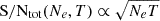 . The form factor, g(Ne), depends on the distribution across time of the observational epochs, which was 1.7 for the continuous monitoring programme that we considered.
Figure 9 shows the acceleration measurement uncertainty,  , achieved with ESPRESSO as a function of the temporal baseline of our experiment, starting from the data already collected, and following up with a monitoring campaign of 10, 100, or 1000 hours of integration time each year. The vertical solid lines denote at what epoch we can achieve a 3σ (or 5σ vertical dotted lines) detection of the cosmological signal in the three cases. The estimates of the required baseline for a detection are also reported in Table 3.
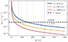 |
Fig. 9. Velocity shift uncertainty reached with ESPRESSO spectra of SB2, as a function of total temporal baseline of the experiment, assuming three different observational strategies with an integration time of 10 hours per year (blue), 100 hours per year (yellow), and 1000 hours per year (red). The horizontal dashed black line defines the magnitude of the cosmological signal expected for a ΛCDM Universe at the average redshift of SB2's Lyman-α forest. Vertical lines define the time needed to achieve a 3σ (solid) and 5σ (dotted) detection for the three observational strategies. |
Temporal baselines required to achieve a 1σ, 3σ, or 5σ detection following up the SB2 spectra with a total integration time of 10, 100, or 1000 hours per year, if performed with ESPRESSO or ANDES (assuming a 10% efficiency).
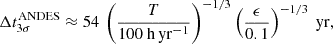
Clearly, the timescales for the experiment are long due to the limited collecting area of VLT. However, these results can be used to estimate, at first order, what the impact will be of moving the observational campaign to the ELT/ANDES spectrograph (Marconi et al. 2024). Assuming that the total efficiencies of the ESPRESSO and ANDES spectrographs are similar (about 10%), since the latter is fed by a telescope with a collecting area ∼20 times larger than the area of one VLT unit, the same accuracy in measuring Δv can be reached in 1/20-th of the total ESPRESSO integration time. By this logic, a 3σ (5σ) detection of the redshift drift can be carried out observing SB2 with ANDES in 68 years (95 years), with 50 hours of total integration time per year, instead of 1000 hours per year as in the case of ESPRESSO.
Similarly, assuming a fixed yearly integration time, the same level of precision in the measurement of the cosmic acceleration  can be achieved with ANDES with a temporal baseline that is a factor 201/3∼2.714 shorter than in the case of an ESPRESSO experiment, due to the scaling of Eq. (13). In this case, a 3σ (5σ) detection of the redshift drift can be carried out by means of a monitoring campaign of SB2 with 100 hours of integration per year, in 54 years (75 years) with ANDES, instead of 145 years (203 years) with ESPRESSO. Table 3 reports the temporal baselines required for detection in an ANDES-based experiment, when allocating 10, 100, or 1000 total hours of exposure per year.
The ANDES spectrograph is yet to be constructed, and its efficiency could change in the future design phases. We can easily parametrise the required baseline of the measurement to reach a 3σ detection, letting the total efficiency of ANDES, ϵ, as a free parameter:
 (14)
(14)
where T is the total integration time of an ANDES-like spectrograph per year of the experiment. The total amount of integration hours needed for a 3σ detection is simply
 (15)
(15)
depending on the amount of telescope time that can be continuously allocated to this project.
9. Results and discussion
We set out to assess the feasibility of measuring the redshift drift signal using Lyman-α forest spectroscopy, based on the highest-quality data available prior to the commissioning of ELT/ANDES. We used new, high-resolution, and high-S/N spectra of the most luminous known quasar in the Universe, J052915.80-435152.0 (SB2; zem = 3.962), obtained with ESPRESSO at the VLT. This exceptionally bright object is especially suited to perform the Sandage test of cosmic redshift drift, owing to its luminosity and emission redshift. We began this decades-long experiment with the ultra-stable spectrograph ESPRESSO over a one-year baseline. The primary goal is to investigate the measurement's intrinsic systematics and validate the predictions on the expected total integration time required to achieve a statistically significant detection. This work presents the first two epochs of the experiment, intended to serve as an anchor for comparison to future observations, initially carried out with ESPRESSO and subsequently with ELT/ANDES.
Our main results are:
-
Applying the pixel-by-pixel method of Bouchy et al. (2001) (Sect. 5), we measured a velocity shift between two epochs of Δv=−2.67±6.64 m s−1. These uncertainties are 65% above the prediction made by Liske et al. (2008) (σv,Liske = 4.02 m s−1, see Eq. (5)).
-
Using an ensemble of 500 models specifically tailored to the resolution, pixel size, and S/N of our data (Sect. 6), we identified spectral regions more sensitive to velocity shifts and gave them more weight in our analysis, obtaining
 . This is a 30% improvement in statistical uncertainty over the direct method, and only 10% greater than the value predicted by Liske et al. (2008).
 -
The redshift drift measured between the two epochs turns out to be
 at 〈z〉 = 3.57, which represents the main result of this paper. This value is fully consistent with the value expected within the ΛCDM model, −6.6×10⁻¹¹ yr−1. The quoted uncertainties are only statistical and three orders of magnitude larger than the cosmological signal. Systematic uncertainties due to the motion of the Solar System, temporal variability of SB2's luminosity, and wavelength calibration are currently sub-dominant.
 -
Based on these findings, we estimate that a 3σ detection of the redshift drift could be achieved with ESPRESSO (ANDES) after 145 (54) years, assuming 100 hours of observation per year for SB2 (Table 3).
The best current upper limit on cosmic acceleration is  at a 1σ confidence level (Darling 2012). Our measurement of
  translates into
 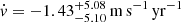 (Sect. 6), making our limit a factor of 2.3 larger than that of Darling (2012). However, their result is based on observations of H I 21 cm absorption line systems in ten objects over a baseline of 13 years, while we obtained a comparable result with only 12.4h of Lyman-α forest and a ∼1 year baseline. By expanding our dataset by another 12 hours over the next 1.5 years, we expect to match the uncertainty in the measurement of Darling (2012), showcasing the power of Lyman-α observations for ż measurements.
Interestingly, neither the pixel-by-pixel method (Sect. 5) nor our newly developed method based on splines (Sect. 6) precisely reproduce the uncertainties predicted by the scaling relation of Liske et al. (2008). This discrepancy may arise because the Liske et al. (2008) relation was calibrated assuming a measurement carried out on a sample of multiple objects, whereas we analysed a single sightline. Sightline-to-sightline fluctuations in the measurement uncertainties are expected due to cosmic variance, where the analysis of SB1 will provide further insights into this issue (Marques et al., in prep.).
We examined the validity of our methods and some potential sources of systematic uncertainties in Sect. 7. While both the direct and the spline methods recover simulated Δv (within uncertainties) for |Δv|<5 m s−1, the pixel-by-pixel method shows a systematic underestimation of the shift when recovering the simulated |Δv|≈40 m s−1 (Fig. 7). Such a result is not currently understood. Solar System accelerations add ∼1 cm s−1 yr−1 to the expected signal, being negligible at the current level of S/N. The presence of such an effect does not alter the experiment's expected temporal baseline (see Sect. 7.4). Excluding the quasar proximity zone from our analysis shifts Δv by 5.14 m s−1, a value only marginally inconsistent (∼1.01σ) with the statistical uncertainty (Sect. 7.3). The shift is likely a consequence of a large (10%) decrease in the number of available pixels, and not a true estimate of uncertainty from quasar variability. More data and longer time baselines are needed to confirm whether temporal variability in quasar flux causes a systematic effect on Δv. Wavelength calibration uncertainties are estimated to be ≈1 m s−1 (Sect. 7.5). Considering the latter is approximately one fourth of the statistical uncertainty, we expect that systematic effects will start playing a significant role in the error budget (in SB2 measurements) once the total S/N quadruples (see Eq. (5)).
A caveat of both methods used in this paper is that they are unable to disentangle a real velocity shift in the data from any changes to the instrument properties, such as its LSF. The LSF is known to change when important components are replaced (Lo Curto et al. 2015), and is likely to occur in experiments spanning several decades. There were no major interventions in ESPRESSO over the time period spanning observations presented here that would raise concerns about LSF or other instrument properties varying. However, removing instrumental imprints will be important in the future; for example, by employing advanced data reduction frameworks such as ‘spectro-perfectionism’ (Bolton & Schlegel 2010) or similar (Piskunov et al. 2021).
Based on considerations presented in Sect. 8, a 3σ detection of ż using SB2 will require 54 years of observations with ANDES when allocating 12.5 nights per year to this project (Table 3). Shorter timescales can be achieved with a more intensive campaign or by increasing the total efficiency of ANDES (see Eq. (14)). For obvious reasons, an intensive monitoring campaign of such magnitude focusing on only one object is not ideal. In a more realistic case, multiple bright objects will be observed simultaneously, spread over a large range of right ascensions. A golden sample of seven quasars compiled with this goal in mind has already been proposed by Cristiani et al. (2023). In such a case, SB2 being the brightest quasar of the sample, the experiment baseline will slightly increase with respect to Eq. (14) at fixed total observational cadence, T, with time shared among multiple targets. However, the other quasar's sightline might be better suited for the test, with more narrow lines, fewer strong absorbers, and a larger fraction of the forest available for the measurement than what we found on SB2. A measurement on such sightlines would have smaller uncertainties and counterbalance the lower S/N related to the fainter objects. At this level, it is not straightforward to formally predict the consequences of such effects on the baseline of an experiment involving all seven quasars of the golden sample. In a parallel paper (Marques et al, in prep.), we shall analyse the spectrum of SB1, the second brightest object of the sample, in order to address this point.
Data availability
Table A.1 is available at the CDS via anonymous ftp to cdsarc.cds.unistra.fr (130.79.128.5) or via https://cdsarc.cds.unistra.fr/viz-bin/cat/J/A+A/699/A159
Acknowledgments
AT is grateful to Vid Iršič for the prolific discussions. The INAF authors acknowledge financial support of the Italian Ministry of Education, University, and Research with PRIN 201278X4FL and the “Progetti Premiali” funding scheme. This work was financed by Portuguese funds through FCT (Fundação para a Ciência e a Tecnologia) in the framework of the project 2022.04048.PTDC (Phi in the Sky, DOI 10.54499/2022.04048.PTDC). CJM also acknowledges FCT and POCH/FSE (EC) support through Investigador FCT Contract 2021.01214.CEECIND/CP1658/CT0001 (DOI 10.54499/2021.01214.CEECIND/CP1658/CT0001). CMJM is supported by an FCT fellowship, grant number 2023.03984.BD. MTM acknowledges the support of the Australian Research Council through Future Fellowship grant FT180100194 and through the Australian Research Council Centre of Excellence in Optical Microcombs for Breakthrough Science (project number CE230100006) funded by the Australian Government. TMS acknowledges the support from the SNF synergia grant CRSII5-193689 (BLUVES). The work of KB is supported by NOIRLab, which is managed by the Association of Universities for Research in Astronomy (AURA) under a cooperative agreement with the U.S. National Science Foundation. EP acknowledges financial support from the Agencia Estatal de Investigación of the Ministerio de Ciencia e Innovación MCIN/AEI/10.13039/501100011033 and the ERDF “A way of making Europe” through project PID2021-125627OB-C32, and from the Centre of Excellence “Severo Ochoa” award to the Instituto de Astrofisica de Canarias. ASM and JIGH acknowledge financial support from the Spanish Ministry of Science, Innovation and Universities (MICIU) projects PID2020-117493GB-I00 and PID2023-149982NB-I00. NS and NN acknowledge financial support by FCT - Fundação para a Ciência e a Tecnologia through national funds by these grants: UIDB/04434/2020 DOI: 10.54499/UIDB/04434/2020, UIDP/04434/2020 DOI: 10.54499/UIDP/04434/2020. FP would like to acknowledge the Swiss National Science Foundation (SNSF) for supporting research with ESPRESSO through the SNSF grants nr. 140649, 152721, 166227, 184618 and 215190. The ESPRESSO Instrument Project was partially funded through SNSF's FLARE Programme for large infrastructures.
The terminology “Super Bright quasars” used in this paper is purely chronological and does not reflect hierarchy based on luminosity, originating from the observation sequence: J212540.97 was identified at an earlier stage in the QUBRICS survey and is designated as SB1, whereas the brighter J052915.80 was discovered later.
Using higher order splines does not affect the results of the analysis.
References
- Adame, A. G., Aguilar, J., Ahlen, S., et al. 2025, JCAP, 2025, 021 [CrossRef] [Google Scholar]
- Albrecht, A., Bernstein, G., Cahn, R., et al. 2006, arXiv e-prints [astro-ph/0609591] [Google Scholar]
- Alves, C. S., Leite, A. C. O., Martins, C. J. A. P., Matos, J. G. B., & Silva, T. A. 2019, MNRAS, 488, 3607 [NASA ADS] [CrossRef] [Google Scholar]
- Becker, G. D., & Bolton, J. S. 2013, MNRAS, 436, 1023 [Google Scholar]
- Bolton, A. S., & Schlegel, D. J. 2010, PASP, 122, 248 [NASA ADS] [Google Scholar]
- Bolton, J. S., Puchwein, E., Sijacki, D., et al. 2017, MNRAS, 464, 897 [NASA ADS] [CrossRef] [Google Scholar]
- Bouchy, F., Pepe, F., & Queloz, D. 2001, A&A, 374, 733 [NASA ADS] [CrossRef] [EDP Sciences] [Google Scholar]
- Calderone, G., Boutsia, K., Cristiani, S., et al. 2019, ApJ, 887, 268 [NASA ADS] [CrossRef] [Google Scholar]
- Cooke, R. 2020, MNRAS, 492, 2044 [Google Scholar]
- Cristiani, S., Porru, M., Guarneri, F., et al. 2023, MNRAS, 522, 2019 [NASA ADS] [CrossRef] [Google Scholar]
- Cristiani, S., Cupani, G., Trost, A., et al. 2024, MNRAS, 528, 6845 [Google Scholar]
- Cupani, G., D’Odorico, V., Cristiani, S., et al. 2016, in Software and Cyberinfrastructure for Astronomy IV, eds. G. Chiozzi, & J. C. Guzman, SPIE Conf. Ser., 9913, 99131T [Google Scholar]
- Cupani, G., D’Odorico, V., Cristiani, S., et al. 2020, in Software and Cyberinfrastructure for Astronomy VI, eds. J. C. Guzman, & J. Ibsen, Int. Soc. Opt. Photon. (SPIE), 11452, 372 [Google Scholar]
- Darling, J. 2012, ApJ, 761, L26 [Google Scholar]
- Dawson, K. S., Schlegel, D. J., Ahn, C. P., et al. 2013, AJ, 145, 10 [Google Scholar]
- Dawson, K. S., Kneib, J. -P., Percival, W. J., et al. 2016, AJ, 151, 44 [NASA ADS] [CrossRef] [Google Scholar]
- Di Marcantonio, P., Sosnowska, D., Cupani, G., et al. 2018, in Observatory Operations: Strategies, Processes, and Systems VII, SPIE Conf. Ser., 10704, 107040F [Google Scholar]
- Fienga, A., Manche, H., Laskar, J., Gastineau, M., & Verma, A. 2014, arXiv e-prints [1405.0484] [Google Scholar]
- Gaia Collaboration (Brown, A. G. A., et al.) 2021, A&A, 649, A1 [NASA ADS] [CrossRef] [EDP Sciences] [Google Scholar]
- Garnavich, P. M., Kirshner, R. P., Challis, P., et al. 1998, ApJ, 493, L53 [Google Scholar]
- Heinesen, A. 2021, Phys. Rev. D, 103, L081302 [Google Scholar]
- Inoue, T., Komatsu, E., Aoki, W., et al. 2020, PASJ, 72, L1 [Google Scholar]
- Kang, J., Zhang, T. -J., He, P., & Zhu, M. 2025, ApJ, 982, 177 [Google Scholar]
- Kim, T. S., Carswell, R. F., Cristiani, S., D’Odorico, S., & Giallongo, E. 2002, MNRAS, 335, 555 [NASA ADS] [CrossRef] [Google Scholar]
- Klöckner, H. R., Obreschkow, D., Martins, C., et al. 2015, PoS, AASKA14, 027 [Google Scholar]
- Lee, C. -C., Webb, J. K., Milaković, D., & Carswell, R. F. 2021, MNRAS, 507, 27 [NASA ADS] [CrossRef] [Google Scholar]
- Liske, J., Grazian, A., Vanzella, E., et al. 2008, MNRAS, 386, 1192 [NASA ADS] [CrossRef] [Google Scholar]
- Lo Curto, G., Pepe, F., Avila, G., et al. 2015, The Messenger, 162, 9 [NASA ADS] [Google Scholar]
- Loeb, A. 1998, ApJ, 499, L111 [NASA ADS] [CrossRef] [Google Scholar]
- Marconi, A., Abreu, M., Adibekyan, V., et al. 2024, in Ground-based and Airborne Instrumentation for Astronomy X, eds. J. J. Bryant, K. Motohara, & J. R. D.Vernet, SPIE Conf. Ser., 13096, 1309613 [Google Scholar]
- Marques, C. M. J., Martins, C. J. A. P., & Alves, C. S. 2023, MNRAS, 522, 5973 [Google Scholar]
- Marques, C. M. J., Martins, C. J. A. P., & Gilabert López, B. 2024, MNRAS, 527, 9918 [Google Scholar]
- Martins, C. J. A. P., et al. 2024, Exper. Astron., 57, 5 [Google Scholar]
- McVittie, G. C. 1962, ApJ, 136, 334 [Google Scholar]
- Milaković, D., Webb, J. K., Molaro, P., et al. 2024, MNRAS, 534, 12 [Google Scholar]
- Noll, S., Kausch, W., Kimeswenger, S., et al. 2014, A&A, 567, A25 [NASA ADS] [CrossRef] [EDP Sciences] [Google Scholar]
- Onken, C. A., Wolf, C., Bessell, M. S., et al. 2024, PASA, 41 [Google Scholar]
- Pepe, F., Cristiani, S., Rebolo, R., et al. 2021, A&A, 645, A96 [NASA ADS] [CrossRef] [EDP Sciences] [Google Scholar]
- Péroux, C., McMahon, R. G., Storrie-Lombardi, L. J., & Irwin, M. J. 2003, MNRAS, 346, 1103 [Google Scholar]
- Piskunov, N., Wehrhahn, A., & Marquart, T. 2021, A&A, 646, A32 [NASA ADS] [CrossRef] [EDP Sciences] [Google Scholar]
- Planck Collaboration VI. 2020, A&A, 641, A6 [NASA ADS] [CrossRef] [EDP Sciences] [Google Scholar]
- Quercellini, C., Amendola, L., Balbi, A., Cabella, P., & Quartin, M. 2012, Phys. Rept., 521, 95 [Google Scholar]
- Rauch, M. 1998, ARA&A, 36, 267 [Google Scholar]
- Riess, A. G., Filippenko, A. V., Challis, P., et al. 1998, AJ, 116, 1009 [Google Scholar]
- Riess, A. G., Casertano, S., Yuan, W., et al. 2021, ApJ, 908, L6 [NASA ADS] [CrossRef] [Google Scholar]
- Rocha, B. A. R., & Martins, C. J. A. P. 2022, MNRAS, 518, 2853 [Google Scholar]
- Rorai, A., Becker, G. D., Haehnelt, M. G., et al. 2017, MNRAS, 466, 2690 [Google Scholar]
- Sandage, A. 1962, ApJ, 136, 319 [CrossRef] [Google Scholar]
- Schmidt, T. M. 2024, MNRAS, 532, 1635 [Google Scholar]
- Schmidt, T. M., Molaro, P., Murphy, M. T., et al. 2021, A&A, 646, A144 [NASA ADS] [CrossRef] [EDP Sciences] [Google Scholar]
- Trost, A., Bolton, J. S., Caputo, A., et al. 2025, Phys. Rev. D, 111, 083034 [Google Scholar]
- Uzan, J. -P., Clarkson, C., & Ellis, G. F. R. 2008, Phys. Rev. Lett., 100, 191303 [Google Scholar]
- Vernet, J., Dekker, H., D’Odorico, S., et al. 2011, A&A, 536, A105 [NASA ADS] [CrossRef] [EDP Sciences] [Google Scholar]
- Webb, J. K., Lee, C. C., Milaković, D., et al. 2025, MNRAS, 539, L1 [Google Scholar]
- Wolf, C., Lai, S., Onken, C. A., et al. 2024, Nat. Astron., 8, 520 [Google Scholar]
- Wright, J. T., & Eastman, J. D. 2014, PASP, 126, 838 [Google Scholar]
All Tables
Summary of single observing blocks (OBs) of SB2 taken during observing periods P110 and P112.
Temporal baselines required to achieve a 1σ, 3σ, or 5σ detection following up the SB2 spectra with a total integration time of 10, 100, or 1000 hours per year, if performed with ESPRESSO or ANDES (assuming a 10% efficiency).
All Figures
|
Fig. 1. Combined spectrum of SB2. Top panel: Flux density in arbitrary units is shown in black, with the dashed purple line denoting the flux density error. Bottom panel: S/N per 1 km s−1 pixel. The shaded green area highlights the Lyman-α forest considered in the redshift drift measurement, bound by the Lyman-α and Lyman-β emissions of the quasar, namely between 509−603 m. |
| In the text | |
|
Fig. 2. Normalised transmitted flux of the Lyman-α forest in the combined spectrum of SB2 as a function of wavelength. The solid light blue line highlights the spectral regions masked due to metal absorption, the sub-DLA and bad pixels. The solid purple line reports the flux error. |
| In the text | |
|
Fig. 3. Distribution of the S/N per pixel in the Lyman-α forest of the three spectra of SB2 (dashed red) and of the corresponding mock spectra (solid black). Upper panel: First epoch. Middle panel: Second epoch. Bottom panel: Combined spectrum. |
| In the text | |
|
Fig. 4. Standard deviation of the fit residuals between the combined mock spectra's flux and the spline model with internodal distance A. The blue squares describe the σR of models on different mock spectra and randomly drawn initial node phase ϕ. The black error bars define the average and standard deviation of σR(A)−1. The vertical dashed purple line denotes the optimal value of A. |
| In the text | |
|
Fig. 5. Section of the SB2 spectrum. Top panel: Normalised flux of the first epoch (green), second epoch (orange), and combined (purple) spectra. The mean model, |
| In the text | |
|
Fig. 6. Posterior probability distributions obtained by the MCMC analysis comparing the mean model to the spectra of epoch 1 (filled green) and epoch 2 (orange) through the likelihood defined in Eq. (11) (see Sect. 6.4). Scatter points with error bars define the median values and the 68% confidence intervals. |
| In the text | |
|
Fig. 7. Velocity shift, Δv, measured on ten random mock sightline pairs with both the pixel-by-pixel (blue square scatter points, see Sect. 5) and model-based methods (red diamond scatter points, see Sect. 6.4) where a different baseline is assumed between the two epochs. The horizontal blue dotted and dashed red lines report the average Δv measured with the pixel-by-pixel and the model-based methods, respectively. From left to right, the mock datasets are built assuming no shift (Δvexp = 0 m s−1), Δt = 0.875 yr (the same time elapsed between the two observed spectra, Δvexp=−0.38 cm s−1), Δt = 103 yr (Δvexp=−4.3 m s−1), and Δt = 104 yr (Δvexp=−42.9 m s−1). The dashed grey lines report the assumed shift. |
| In the text | |
|
Fig. 8. Estimated velocity shift, Δv, computed on ten equispaced sections of the Lyman-α forest. Top panel: Δv estimated on each spectral chunk with the pixel-by-pixel (blue squares) and model-based (red diamonds) methods, as a function of the section's central wavelength λc. Middle panel: Measurement uncertainty, σv, for the two methods, shown with the same colour coding as the panel above. The dash-dotted and dashed grey lines report the expected uncertainty of the two methods, based on the median S/N and pixel number of each chunk. Bottom panel: Fraction of the Lyman-α forest |
| In the text | |
|
Fig. 9. Velocity shift uncertainty reached with ESPRESSO spectra of SB2, as a function of total temporal baseline of the experiment, assuming three different observational strategies with an integration time of 10 hours per year (blue), 100 hours per year (yellow), and 1000 hours per year (red). The horizontal dashed black line defines the magnitude of the cosmological signal expected for a ΛCDM Universe at the average redshift of SB2's Lyman-α forest. Vertical lines define the time needed to achieve a 3σ (solid) and 5σ (dotted) detection for the three observational strategies. |
| In the text | |
Current usage metrics show cumulative count of Article Views (full-text article views including HTML views, PDF and ePub downloads, according to the available data) and Abstracts Views on Vision4Press platform.
Data correspond to usage on the plateform after 2015. The current usage metrics is available 48-96 hours after online publication and is updated daily on week days.
Initial download of the metrics may take a while.