| Issue |
A&A
Volume 688, August 2024
|
|
|---|---|---|
| Article Number | L26 | |
| Number of page(s) | 9 | |
| Section | Letters to the Editor | |
| DOI | https://doi.org/10.1051/0004-6361/202450798 | |
| Published online | 14 August 2024 | |
Letter to the Editor
Damping wings in the Lyman-α forest: A model-independent measurement of the neutral fraction at 5.4 < z < 6.1
1
Institute for Theoretical Physics, Heidelberg University, Philosophenweg 12, 69120 Heidelberg, Germany
2
Max-Planck-Institut für Astronomie, Königstuhl 17, 69117 Heidelberg, Germany
3
Steward Observatory, University of Arizona, 933 North Cherry Avenue, Tucson, AZ 85721, USA
4
Department of Physics & Astronomy, University of California, Riverside, CA 92521, USA
Received:
20
May
2024
Accepted:
24
July
2024
Abstract
Context. Recent observations have positioned the end point of the Epoch of Reionization (EoR) at a redshift of z ∼ 5.3. However, observations of the Lyman-α forest have not yet been able to discern whether reionization occurred slowly and late, with substantial neutral hydrogen persisting at a redshift of ∼6, or rapidly and earlier, with the apparent late end driven by the fluctuating ultraviolet background. Gunn-Peterson (GP) absorption troughs are solid indicators that reionization is not complete until z = 5.3, but whether they contain significantly neutral gas has not yet been proven.
Aims. We aim to answer this question by directly measuring, for the first time, the neutral hydrogen fraction (xHI) at the end of the EoR (5 ≲ z ≲ 6) in high-redshift quasar spectra.
Methods. For high neutral fractions, xHI ≳ 0.1, GP troughs exhibit damping wing (DW) absorption extending over 1000 km s−1 beyond the troughs. While conclusively detected in Lyman-α emission lines of quasars at z ≥ 7, DWs are challenging to observe in the general Lyman-α forest due to absorption complexities and small-scale stochastic transmission features.
Results. We report the first successful identification of the stochastic DW signal adjacent to GP troughs at redshifts of z = 5.6 through careful stacking of the dark gaps in the Lyman-α forest (S/N = 6.3). We use the signal to present a measurement of the corresponding global xHI = 0.19 ± 0.07 (−0.16+0.11) at 1σ (2σ) at z = 5.6 and a limit of xHI < 0.44 at z = 5.9.
Conclusions. The detection of this signal demonstrates the existence of substantially neutral islands near the conclusion of the EoR, unequivocally signaling a late-and-slow reionization scenario.
Key words: intergalactic medium / quasars: absorption lines / dark ages, reionization, first stars
Corresponding author; This email address is being protected from spambots. You need JavaScript enabled to view it. .
© The Authors 2024
 Open Access article, published by EDP Sciences, under the terms of the Creative Commons Attribution License (https://creativecommons.org/licenses/by/4.0), which permits unrestricted use, distribution, and reproduction in any medium, provided the original work is properly cited.
This article is published in open access under the Subscribe to Open model. This email address is being protected from spambots. You need JavaScript enabled to view it. to support open access publication.
1. Introduction
The Gunn-Peterson (GP) effect is pivotal to constraining the Epoch of Reionization (EoR); that is, the transition of the intergalactic medium (IGM) from a predominantly neutral state to an ionized one (Gunn & Peterson 1965). The effect is observed as “GP troughs” showing nearly complete absorption of rest-frame 1215.67 Å photons by neutral hydrogen with an H I fraction of xHI ≳ 10−4 along the lines of sight to background quasars (Fan et al. 2006; Becker et al. 2015; Bosman et al. 2022). Gunn-Peterson troughs more than 30 cMpc in length are found in the spectra of more than half of quasars at z > 5.7 and persist down to z = 5.3 (Zhu et al. 2021), an observation that rules out a uniformly ionized Universe. However, whether those GP troughs correspond to significantly “neutral islands” of gas with xHI ≃ 1 or to fluctuations in the ultraviolet ionizing background (UVB) in near-fully ionized gas with xHI ≲ 0.01 at z = 6 is still unknown (Gaikwad et al. 2023; Davies et al. 2024). The most stringent upper limit on xHI, based on the total absorbed fraction of the Lyman-α (Lyα) forest, permits xHI < 0.6 at z = 6 (McGreer et al. 2015), while the most stringent lower limit from the Lyα forest at this redshift is xHI > 7 × 10⁻⁵ from fluctuations in the optical depth (Bosman et al. 2022). Models of the end of reionization between these extremes have until now remained indistinguishable.
At high neutral fractions of xHI ≳ 0.1, GP troughs start exhibiting absorption in damping wings (DWs) extending over 1000 km s−1 beyond the troughs themselves. This DW absorption has been detected conclusively over the Lyα emission lines of quasars when the neutral gas is located relatively close to them, giving the first and most robust detections of reionization-related neutral IGM gas (xHI ∼ 0.5) at z ≥ 7 (Mortlock et al. 2011; Davies et al. 2018; Greig et al. 2022). However, DWs cannot be detected on an individual basis in the general Lyα forest due to (1) significant absorption throughout the forest at z > 5 and (2) strong small-scale stochastic transmission features (“transmission spikes”). In this Letter, we present a successful detection of the DW signal around GP troughs at z = 5.6 and z = 5.9 from stacking of GP troughs in the Lyα forest, an idea first proposed by Malloy & Lidz (2015). A detection and measurement of the corresponding necessary global xHI is made possible by the great increase in data quality and quantity from the XQR-30 survey (D’Odorico et al. 2023) and by several improvements to the originally proposed method.
In Sect. 2, we present our observational sample consisting of 38 X-shooter spectra of quasars at 5.4 < z < 6.5. Our method is described in Sect. 3, including GP trough identification (3.1) and stacking (3.2) and xHI estimation (3.3). We present our measurements of the global xHI fraction at z = 5.6 and a limit at z = 5.9 in Sect. 4. Throughout the Letter, we use a Planck flat LCDM cosmology (Planck Collaboration VI 2020), distances are given in comoving units, and xHI is volume-averaged.
2. Sample
Our observational sample consists of 38 X-shooter spectra selected from Bosman et al. (2022). We require the quasars to lie in the redshift range of 5.4 < z < 6.5 and to have a minimum signal-to-noise ratio (S/N) of > 20 per 10 km s−1 pixel. The resolution of the spectra is ∼34 km s−1 over the Lyα forest (see D’Odorico et al. 2023). A list of the quasars in the sample with redshifts and S/N is presented in Appendix A.
The Lyα and Lyman-β (Lyβ) forests of the quasars were normalized using reconstructed underlying continua, as is described in Bosman et al. (2022) and Zhu et al. (2022), which employ the same spectral regions of the same spectra. We used a near-linear log-PCA approach based on the method of Davies et al. (2018), with the improvements described in Bosman et al. (2021).
3. Methods
The Lyα forest saturates at the mean cosmic density as soon as the neutral fraction of the absorbing gas reaches xHI = 10−4. However, multiple models predict that the GP troughs observed down to z = 5.3 are highly neutral, with xHI > 0.1 (Kulkarni et al. 2019). While saturation of the forest on its own is not sensitive in this regime, such large column densities of neutral gas should start to produce DWs out to large velocity separations, Δv > 1000 km s−1 from the GP troughs. While Lyα transmission is too highly stochastic to allow one to observe DWs around individual troughs, in theory the mean neutral fraction of GP troughs can be recovered through the detection of the DW in a deep stack of spectra – a method first suggested theoretically by Malloy & Lidz (2015). We are now in a position to detect this signal in practice for the first time. We largely followed the method outlined by those authors, with changes specifically noted.
In order to select and stack absorption gaps that potentially contain neutral gas, we searched for regions of the forest that are fully absorbed in both Lyα and Lyβ. Those gaps were then stacked using the edge of the Lyβ trough as a point of alignment. Indeed, transmission in the Lyβ forest (or any other higher-order forest) indicates that the gas is not opaque at the Lyman limit; that is, it cannot constitute a damped Lyα absorber (DLA). Since accurate methods of reconstructing the intrinsic quasars continua are not available beyond the Lyβ forest, we do not use higher-order transitions in this Letter.
3.1. Gap finding
First, we excluded an ∼5000 km s−1 region on the blue side of the Lyα (Lyβ) emission line. This exclusion window was sufficient for all but three quasars, where we manually extended the masked region due to unusually long proximity effects.
In order to identify absorbed regions in both the Lyα and Lyβ forests, we must contend with (at least) two sources of contamination: sky-line residuals that may artifically “split” the gaps, and DLAs, which are known to be associated with galactic metal systems rather than the IGM. Our spectra contain residuals due to the removal of sky lines. Under the assumption that sky-line residual spikes are narrow and affect only a limited number of adjacent pixels, and that the genuine transmission spikes will have an S/N per pixel of at least 2.5, we cleaned our signal of sky-line residuals in the following way. First, we smoothed the spectrum with a Gaussian filter with a width of 2 pixels, and compared the smoothed and unsmoothed signals. If the difference between the smoothed and unsmoothed signal exceeded 2.5 times the observational uncertainty at any pixel, we considered it to be affected by sky-line residuals. We then replaced the value of the contaminated pixel with the value of the smoothed signal (re-computed after masking). In this way, pixels most likely to be intrinsically absorbed were assumed to be opaque, and pixels more likely to be transmissive were given flux marking them as not being gaps.
We then identified statistically significant absorbed gaps and determined their edges. The flux distribution of the cleaned signal reveals two distinct features: firstly, a Gaussian-like distribution centered around zero, representing expected fluctuations in the spectral noise; and secondly, a broader distribution reaching higher flux values, indicative of transmission peaks. Utilizing the Gaussian-like noise distribution, we established a threshold for significant detection, denoted as ν. Peaks in the broader distribution are considered genuine if they exhibit an S/N per pixel of at least three compared to the noise distribution.
Further contamination arises from galactic DLA systems along the line of sight, which may be mistaken for GP troughs. We used the catalog of metal absorbers identified by (Davies et al. 2023) to exclude any gaps that are potentially galactic DLAs. We excluded gaps in Lyα that could be caused by either low-ionization or high-ionization systems, and gaps in Lyβ that could be caused by lower-redshift Lyα absorption from low-ionization systems. We retained low-redshift, high-ionization systems that would affect the Lyβ forest alone, since they are very numerous and typically only have modest Lyα absorption, and since their effects do not mimic the signal we are looking for; they only potentially increase the stochastic noise.
Finally, we identified which gaps to stack. We started with all of the foreground regions that were opaque in both Lyα and Lyβ. To increase the sensitivity of the measurement, we modified the approach of Malloy & Lidz (2015) to use both sides of such gaps (red and blue), since DWs are expected to affect both nearly equally. Further, we tried to mitigate the effect of contamination of the Lyβ forest by overlapping lower-redshift Lyα absorption. We note that there is no physical reason, other than contamination, for the Lyβ forest to saturate while Lyα does not. We therefore excluded from the stack all gap edges that are “terminated” or split by Lyα transmission, since that fact makes it clear that the gap has run into highly ionized gas.
In Fig. 1, we illustrate our gap-finding algorithm for a single sight line. The Lyα and Lyβ spectra are shown with colored bands indicating identified gaps. We identify in gray the gaps that were excluded due to corresponding to potential DLAs identified through metal absorption, while the white regions are not gaps (i.e. transmission spikes, or the quasar proximity zone).
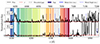 |
Fig. 1. Example of the gap-finding procedure for the sight line toward quasar ATLAS J029.9915−36.5658. The Lyα (bottom) and Lyβ (top) spectra are depicted along with identified gaps (colored bands). Contamination from metal systems is also displayed (vertical blue lines) and corresponding gaps have been removed (gray-strip bands). In this example, a high-ionization metal system potentially affecting the Lyα forest is identified, leading to the removal of three joint gaps. |
3.2. Gap stacking
We stacked the gaps that we identified, as is outlined above. The gaps were stacked at their edges, ideally corresponding to the H I/H II region limit. Prior to stacking, we normalized the flux using the global mean flux as a function of redshift, using the functional form given in Bosman et al. (2022). To enhance the robustness of our analysis and expand our sample, we employed a strategy of flipping and stacking the blue edges of the gaps with the red edges. We computed uncertainties through a bootstrap procedure on the selected gaps.
We explored the redshift dependence of the H I fraction by dividing our sample into two redshift bins, 5.4 ≤ z < 5.8 (⟨z⟩ = 5.67) and 5.8 ≤ z < 6.1 (⟨z⟩ = 5.89). Following the methodology established in Malloy & Lidz (2015), we began by comparing stacks of the Lyα forest around “short” and “long” gaps. The rationale behind this comparison lies in the expectation that short gaps, originating from H II regions, should contain minimal H I content. By contrast, we anticipate long gaps to exhibit an excess of H I.
Short gaps were defined as those with a velocity width less than 200 km s−1, while long gaps were determined by a threshold parameter, Lthres. A higher value of Lthres limits the stack to longer gaps that are more likely to be highly neutral, but at the cost of the sample size. In the analysis of the signal below, we usually marginalized over Lthres in order to remain agnostic as to the minimum length of gaps that are significantly neutral.
As will be shown in Sect. 4 and Fig. 2, we achieve a detection of the statistical DW signal in the lower-redshift bin at z = 5.6. To interpret this signal without relying on existing model-dependent simulations, we develop a simple analytical framework to estimate the most likely value of the global xHI giving rise to the observations.
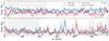 |
Fig. 2. Stacked spectrum around long and short gaps for two redshift bins (top: z = 5.6, bottom: z = 5.9). In each panel, the red and blue curves depict the stacked profiles of long and short gaps, respectively, with their widths being the uncertainties from bootstrap resampling. The continuous light blue line and the dotted orange line indicate the best-fit transmission model fit to the stack around long gaps for the step-function model and the piecewise model, respectively. Long gaps are defined as those with velocity widths greater than 340 km s−1, while short gaps have lengths under 200 km s−1. The curves in the bottom panel show the models that are permitted at a 2σ level. |
3.3. Constraints on the H I fraction
We employed two toy models to capture the distribution of neutral gas among gaps of varying lengths. The simplest model is a step-function relation, whereby gaps longer than a threshold, LC, originate from completely neutral hydrogen, while shorter gaps arise from H II regions. The local H I fraction  of such gaps is given by
 (1)
(1)
In an attempt to make the distribution more realistic, we also explore a piecewise relation. In this model, we allow for a mixture of neutral and ionized hydrogen clouds to populate gaps. The H I fraction,  , of gaps is then given by
 (2)
(2)
We based this model on the findings of Zhu et al. (2022), in which a similar functional form was the best explanation for the observed trough lengths in the Lyα and Lyβ forests. We allowed the mean flux, T, to vary. Since the gaps were normalized by the mean flux at the redshift considered, such a free parameter should not be necessary. However, the strong correlation of the Lyα forest on very large scales around gaps of different lengths prevents the mean flux from converging to 1, as we shall discuss in Sect. 4. The parameter T is dominated by the behavior of the stacked flux at large velocity separations and is tightly constrained, so we hold it fixed at its optimal value rather than marginalizing over it in the analysis.
Both of these simple models contain only one parameter, LC, which is the gap length above which full neutrality of the gas is assumed. For each value of LC, we generated the shape of the expected stacked DW via
![Mathematical equation: $$ \begin{aligned} \langle F \rangle = \left[\left(1 - x_{\rm HI}^L \right) e^{-\tau _D \left(x_{\rm HI}^L = 0\right)} + x_{\rm HI}^L e^{-\tau _D \left(x_{\rm HI}^L = 1\right)}\right]T, \end{aligned} $$](/articles/aa/full_html/2024/08/aa50798-24/aa50798-24-eq6.gif) (3)
(3)
where τD(xHI) is the conventional GP DW optical depth (Mortlock 2016).
We fit this functional shape to the signal using χ2 minimization. We made use of the stacked signal over a velocity range of 150 < Δv < 3000 km s−1 at z = 5.6 and 180 < Δv < 3000 at z = 5.9, but we did not use the signal beyond the Δv where less than 100 spectra were stacked. Since the covariance matrix of the stacked signal contains strong non-diagonal elements that prevent inversion, we performed parameter inference empirically instead. We performed 5000 draws of the stacked signal via bootstrap and obtained posteriors on LC from the distribution of their optima. We then repeated this procedure for a variant of the signal using a different Lthresh, the lower limit for a long gap. Finally, we marginalized over Lthresh to obtain the final posterior on LC.
The central value of LC and its uncertainties can be translated into a global neutral fraction, xHI. To do this, we assigned to each gap used in the analysis its own local neutral fraction according to Eqs. (1) or (2), and we assigned a value, xHI = 0, to the un-masked, non-gap portion of the quasar sight lines. The resulting volume-average is our estimate of the global xHI.
4. Results
4.1. Detection of a statistical damping wing signal
By comparing the stacked Lyα flux around short and long gaps at z = 5.6, we detect a very strong signal at Δv < 500 km s−1 that is consistent with qualitative expectations from a statistical DW (Fig. 2). The decrement is significant at S/N = 6.3, as was determined by re-binning the signal on a matching scale of 80 km s−1 and computing the bootstrap uncertainties on the range. The S/N does not scale well with binning, since the source of the uncertainties is predominantly in cosmic variance. We repeated this procedure for the rest of the stack over the usable velocity range, and found no other features significant at S/N > 4. We show the S/N distributions in Appendix B.
The upturn in transmission around H II regions, predicted by Malloy & Lidz (2015), occurs because the edges of Lyα and Lyβ gaps align when the IGM is ionized and over-dense. This results in the first pixel of the Lyα stack being above the mean flux. The detection of this feature in small gaps confirms they contain mostly ionized gas, while its partial presence in long gaps suggests these gaps either contain ionized gas or are caused by foreground contamination from lower-redshift Lyα absorption in the Lyβ forest.
However, other features and differences are also visible in stacked flux, and were not predicted by, for example, the forecasts of Malloy & Lidz (2015). In the central ∼3 velocity pixels, corresponding to Δv < 150 km s−1, the flux stacks around both the long and short gaps show a clear excess compared to larger separations. We suspect that this is due a large fraction of the gaps having a very low xHI, causing the edges of the Lyα and Lyβ gaps to overlap. For such gaps, the next pixels past the edge of the gap are far more likely to be a spike than in the general IGM, causing the stacked signal to shoot up above the mean. The fact that this boost persists to ∼500 km s−1 in the stack around short gaps indicates that transmission spikes are likely clustered, something which has been theorized and predicted to occur on exactly these scales (Wolfson et al. 2024).
Another unexpected effect is that the mean fluxes around short gaps and long gaps do not converge even up to Δv = 6000 km s−1, corresponding to a distance of 62 Mpc. This is indicative of extremely long correlation scales in Lyα transmission at the end of the EoR, as is hinted at by the existence of individual GP troughs over 110 Mpc in length (Becker et al. 2015). Long gaps are more likely to be located in sight lines that are more opaque than average on large scales.
No difference between the flux stack around short and long gaps is visible at z = 5.9. The mean transmission at this redshift is four times lower than at z = 5.6, as only ∼1% of quasar emission is transmitted in the forest (Bosman et al. 2022). Despite our analysis containing more gaps and gap edges at z = 5.9, the S/N of the stack is most likely not sufficient to detect the signal. We used the z = 5.9 stack to impose a limit on xHI. A similar signal was seen independently by Zhu et al. (2024).
4.2. Implications for the neutral fraction
We used our analytical framework as a first estimate of the rough global xHI required by the strength of the signal. To achieve this, we masked the central 150 km s−1 of the signal and allowed the mean transmission at large separations to vary (T), as was outlined in the previous section. The best fits to the z = 5.6 signal are shown in the top panel of Fig. 2 as solid blue and dashed orange curves, corresponding to a step function and a piecewise function distribution of neutral gas as a function of gap length, respectively. While the two models agree well, they are both relatively poor fits to the shape of the signal. Nevertheless, we propagated the uncertainties to achieve a measurement of xHI = 0.19 ± 0.07  at 1σ (2σ) by taking the mean and the outer envelope of constraints from the step and piecewise functions. We briefly investigated the effect of the maximum fraction of gaps that are neutral being dropped to 75% in the piecewise assumption: we then would recover a value of xHI that is ∼15% higher (but comfortably within our uncertainties). At z = 5.9, the posterior returns an upper limit on xHI < 0.44 at 2σ.
We compare these values to the literature in Fig. 3. While the z = 5.9 limit is broadly consistent with other tracers, the value we find of xHI ∼ 0.2 at z = 5.6 is in mild tension with evidence from dark pixels (McGreer et al. 2015) and the distribution of dark gap lengths (Zhu et al. 2022). A neutral fraction of 20% at z = 5.6 is higher than predicted by models even with ultra-late reionization (Kulkarni et al. 2019; Asthana et al. 2024). We note that, although the shape of the signal appears to be poorly captured by our simple analytic form, the strength of the signal is stronger than our fit (Fig. 2), especially when compared to the stack around short absorption gaps.
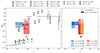 |
Fig. 3. Constraints on the neutral fraction across cosmic time. The solid and dashed colored boxes indicate our 1σ and 2σ constraints, respectively. Right: constraints obtained in this work, in the two redshift bins and with the two xHI − L relations proposed. Left: existing constraints from the literature: McGreer et al. (2015), Greig et al. (2017), Greig et al. (2019), Davies et al. (2018), Mason et al. (2018), Mason et al. (2019), Wang et al. (2020), Yang et al. (2020a,b), Zhu et al. (2022), Bosman et al. (2022), Jin et al. (2023), Zhu et al. (2024). Some of the literature points have been slightly shifted in redshift, and the constraints of Greig et al. (2024) have been combined for improved clarity. |
However, the extra features observed in the z = 5.6 spectral stack suggest that our simple analytical model might not be sufficient to characterize the signal and extract a global neutral fraction. In future work, we shall employ simulation suites to hopefully model the signal and its contamination fully. Still, we note that even the largest existing cosmological simulations struggle to reproduce the very large scales over which coherence in the mean flux is seen, while maintaining a sufficient resolution to reproduce the clustering of transmission spikes. We are looking forward to more detailed modeling in future work.
5. Summary
We conducted a search for DWs inside the Lyα forest at the end of the EoR. Following the method laid out by Malloy & Lidz (2015), we identified IGM regions opaque to both Lyα and Lyβ that may therefore contain significantly neutral gas.
We stacked the Lyα forest past the edge of these dark gaps, identified by the end of the trough in Lyβ. Following Malloy & Lidz (2015), we compare the stacked flux seen around short gaps (length < 200 km s−1) and longer gaps (with a variable threshold; 340 km s−1 is shown in Fig. 2). We find a clear signal consistent with a stacked DW on scales of ∼300 km s−1 around the long gaps and not the short gaps at z = 5.6, but no such signal at z = 5.9 where our S/N is significantly lower.
In addition to the DW signal, the stacked flux around the long gaps also displays two unexpected features: a boost in the very central pixels, which we attribute to contamination by highly ionized gaps, and a systematic shift toward a lower mean flux compared to the short gaps on very large scales of > 60 Mpc, probably due to large-scale correlations in the UVB. These features were not predicted by forecasts of this signal.
We nevertheless attempted to model the stack around long gaps after masking the central contamination boost. We assigned to each gap a neutral fraction as a function of its length via two toy models that give consistent results. The resulting best fit implies a high neutral fraction of xHI = 0.19 ± 0.07, or xHI > 0.03 at 2σ. At z = 5.9, we can only impose an upper limit of xHI < 0.44. While more modeling is needed to understand the complexities of the stacked DW signal, the fact that it is detected at all in the z = 5.6 IGM is an unequivocal sign of the existence of significantly neutral islands at the end of the EoR.
Acknowledgments
The authors thank the helpful anonymous referee who contributed valuable comments which improved the manuscript. BS and SEIB are supported by the Deutsche Forschungsgemeinschaft (DFG) under Emmy Noether grant number BO 5771/1-1. Part of this work is based on observations collected at the European Southern Observatory under ESO programme 1103.A-0817. This work made use of the publicly available software package CORECON (Garaldi 2023).
References
- Asthana, S., Haehnelt, M. G., Kulkarni, G., et al. 2024, ArXiv e-prints [arXiv:2404.06548] [Google Scholar]
- Becker, G. D., Bolton, J. S., Madau, P., et al. 2015, MNRAS, 447, 3402 [Google Scholar]
- Bosman, S. E. I., Ďurovčíková, D., Davies, F. B., & Eilers, A.-C. 2021, MNRAS, 503, 2077 [CrossRef] [Google Scholar]
- Bosman, S. E. I., Davies, F. B., Becker, G. D., et al. 2022, MNRAS, 514, 55 [NASA ADS] [CrossRef] [Google Scholar]
- Davies, F. B., Hennawi, J. F., Bañados, E., et al. 2018, ApJ, 864, 142 [NASA ADS] [CrossRef] [Google Scholar]
- Davies, R. L., Ryan-Weber, E., D’Odorico, V., et al. 2023, MNRAS, 521, 289 [NASA ADS] [CrossRef] [Google Scholar]
- Davies, F. B., Bosman, S. E. I., Gaikwad, P., et al. 2024, ApJ, 965, 134 [NASA ADS] [CrossRef] [Google Scholar]
- D’Odorico, V., Bañados, E., Becker, G. D., et al. 2023, MNRAS, 523, 1399 [CrossRef] [Google Scholar]
- Fan, X., Strauss, M. A., Becker, R. H., et al. 2006, AJ, 132, 117 [NASA ADS] [CrossRef] [Google Scholar]
- Gaikwad, P., Haehnelt, M. G., Davies, F. B., et al. 2023, MNRAS, 525, 4093 [NASA ADS] [CrossRef] [Google Scholar]
- Garaldi, E. 2023, J. Open Source Softw., 8, 5407 [NASA ADS] [CrossRef] [Google Scholar]
- Greig, B., Mesinger, A., Haiman, Z., & Simcoe, R. A. 2017, MNRAS, 466, 4239 [Google Scholar]
- Greig, B., Mesinger, A., & Bañados, E. 2019, MNRAS, 484, 5094 [NASA ADS] [CrossRef] [Google Scholar]
- Greig, B., Mesinger, A., Davies, F. B., et al. 2022, MNRAS, 512, 5390 [NASA ADS] [CrossRef] [Google Scholar]
- Greig, B., Mesinger, A., Bañados, E., et al. 2024, MNRAS, 530, 3208 [NASA ADS] [CrossRef] [Google Scholar]
- Gunn, J. E., & Peterson, B. A. 1965, ApJ, 142, 1633 [Google Scholar]
- Jin, X., Yang, J., Fan, X., et al. 2023, ApJ, 942, 59 [NASA ADS] [CrossRef] [Google Scholar]
- Kulkarni, G., Keating, L. C., Haehnelt, M. G., et al. 2019, MNRAS, 485, L24 [Google Scholar]
- Malloy, M., & Lidz, A. 2015, ApJ, 799, 179 [NASA ADS] [CrossRef] [Google Scholar]
- Mason, C. A., Treu, T., Dijkstra, M., et al. 2018, ApJ, 856, 2 [Google Scholar]
- Mason, C. A., Fontana, A., Treu, T., et al. 2019, MNRAS, 485, 3947 [NASA ADS] [CrossRef] [Google Scholar]
- McGreer, I. D., Mesinger, A., & D’Odorico, V. 2015, MNRAS, 447, 499 [NASA ADS] [CrossRef] [Google Scholar]
- Mortlock, D. 2016, Astrophys. Space Sci. Lib., 423, 187 [NASA ADS] [CrossRef] [Google Scholar]
- Mortlock, D. J., Warren, S. J., Venemans, B. P., et al. 2011, Nature, 474, 616 [Google Scholar]
- Planck Collaboration VI. 2020, A&A, 641, A6 [NASA ADS] [CrossRef] [EDP Sciences] [Google Scholar]
- Wang, F., Davies, F. B., Yang, J., et al. 2020, ApJ, 896, 23 [NASA ADS] [CrossRef] [Google Scholar]
- Wolfson, M., Hennawi, J. F., Bosman, S. E. I., et al. 2024, MNRAS, 531, 3069 [NASA ADS] [CrossRef] [Google Scholar]
- Yang, J., Wang, F., Fan, X., et al. 2020a, ApJ, 897, L14 [Google Scholar]
- Yang, J., Wang, F., Fan, X., et al. 2020b, ApJ, 904, 26 [Google Scholar]
- Zhu, Y., Becker, G. D., Bosman, S. E. I., et al. 2021, ApJ, 923, 223 [NASA ADS] [CrossRef] [Google Scholar]
- Zhu, Y., Becker, G. D., Bosman, S. E. I., et al. 2022, ApJ, 932, 76 [NASA ADS] [CrossRef] [Google Scholar]
- Zhu, Y., Becker, G. D., Bosman, S. E. I., et al. 2024, MNRAS, 533, L49 [NASA ADS] [CrossRef] [Google Scholar]
Appendix A: QSO list
We report in Table the sample selected for the analysis, selected from Bosman et al. (2022).
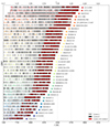 |
Fig. A.1. Overview of dark gaps identified in the Lyα and Lyβ forests from our sample of 38 QSO spectra. Light (dark) gray shaded regions identify the gaps in the Lyα (Lyβ) region. The red shaded regions show the combination of such gaps. |
Sample from Bosman et al. (2022).
Appendix B: Robustness of the DW signal
We test the robustness of the DW signal by looking at the difference between the flux in the long and short gap stacks close to Δν = 0. In Fig. B.1, we display the significance of such flux decrement with different binning windows (W = 40 km s−1, as for our nominal bining scale, and W = 80 km s−1) for the two redshift bins. Our analysis shows that at z ∼ 5.6 there is not another large-flux decrement in the spectrum similar to the one near Δν = 0. An S/N per pixel of ≳6 is found only for 180 km s−1 ≲ Δν ≲ 260 km s−1 at z ∼ 5.6.
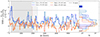 |
Fig. B.1. Significance of the flux decrement near Δν = 0. In the left panel, the S/N per pixel is illustrated for different binning windows for the two redshift bins. The gray shadow area corresponds to the fit region, while FS (σS) and FL (σL) represent the (errors on the) flux of the short and long gaps respectively. The right panel shows the significance distribution within the (gray) fit region. The pixels with an S/N larger than 5 are highlighted. |
All Tables
All Figures
|
Fig. 1. Example of the gap-finding procedure for the sight line toward quasar ATLAS J029.9915−36.5658. The Lyα (bottom) and Lyβ (top) spectra are depicted along with identified gaps (colored bands). Contamination from metal systems is also displayed (vertical blue lines) and corresponding gaps have been removed (gray-strip bands). In this example, a high-ionization metal system potentially affecting the Lyα forest is identified, leading to the removal of three joint gaps. |
| In the text | |
|
Fig. 2. Stacked spectrum around long and short gaps for two redshift bins (top: z = 5.6, bottom: z = 5.9). In each panel, the red and blue curves depict the stacked profiles of long and short gaps, respectively, with their widths being the uncertainties from bootstrap resampling. The continuous light blue line and the dotted orange line indicate the best-fit transmission model fit to the stack around long gaps for the step-function model and the piecewise model, respectively. Long gaps are defined as those with velocity widths greater than 340 km s−1, while short gaps have lengths under 200 km s−1. The curves in the bottom panel show the models that are permitted at a 2σ level. |
| In the text | |
|
Fig. 3. Constraints on the neutral fraction across cosmic time. The solid and dashed colored boxes indicate our 1σ and 2σ constraints, respectively. Right: constraints obtained in this work, in the two redshift bins and with the two xHI − L relations proposed. Left: existing constraints from the literature: McGreer et al. (2015), Greig et al. (2017), Greig et al. (2019), Davies et al. (2018), Mason et al. (2018), Mason et al. (2019), Wang et al. (2020), Yang et al. (2020a,b), Zhu et al. (2022), Bosman et al. (2022), Jin et al. (2023), Zhu et al. (2024). Some of the literature points have been slightly shifted in redshift, and the constraints of Greig et al. (2024) have been combined for improved clarity. |
| In the text | |
|
Fig. A.1. Overview of dark gaps identified in the Lyα and Lyβ forests from our sample of 38 QSO spectra. Light (dark) gray shaded regions identify the gaps in the Lyα (Lyβ) region. The red shaded regions show the combination of such gaps. |
| In the text | |
|
Fig. B.1. Significance of the flux decrement near Δν = 0. In the left panel, the S/N per pixel is illustrated for different binning windows for the two redshift bins. The gray shadow area corresponds to the fit region, while FS (σS) and FL (σL) represent the (errors on the) flux of the short and long gaps respectively. The right panel shows the significance distribution within the (gray) fit region. The pixels with an S/N larger than 5 are highlighted. |
| In the text | |
Current usage metrics show cumulative count of Article Views (full-text article views including HTML views, PDF and ePub downloads, according to the available data) and Abstracts Views on Vision4Press platform.
Data correspond to usage on the plateform after 2015. The current usage metrics is available 48-96 hours after online publication and is updated daily on week days.
Initial download of the metrics may take a while.