| Issue |
A&A
Volume 559, November 2013
|
|
|---|---|---|
| Article Number | A85 | |
| Number of page(s) | 19 | |
| Section | Cosmology (including clusters of galaxies) | |
| DOI | https://doi.org/10.1051/0004-6361/201322130 | |
| Published online | 19 November 2013 | |
The one-dimensional Lyα forest power spectrum from BOSS⋆
1
CEA, Centre de Saclay, Irfu/SPP,
91191
Gif-sur-Yvette,
France
e-mail:
This email address is being protected from spambots. You need JavaScript enabled to view it.
2
INAF, Osservatorio Astronomico di Trieste, via G. B. Tiepolo 11,
34131
Trieste,
Italy
3
INFN/National Institute for Nuclear Physics,
via Valerio 2,
34127
Trieste,
Italy
4
APC, Université Paris Diderot-Paris 7, CNRS/IN2P3, CEA,
Observatoire de Paris, 10 rue A.
Domon & L. Duquet, 75205
Paris,
France
5
Lawrence Berkeley National Laboratory,
1 Cyclotron Road,
Berkeley, CA
94720,
USA
6
Bruce and Astrid McWilliams Center for Cosmology, Carnegie Mellon
University, Pittsburgh, PA
15213,
USA
7
Department of Physics and Astronomy, University of
Utah, 115 S 1400 E,
Salt Lake City, UT
84112,
USA
8
Institute of Theoretical Physics, University of Zurich,
8057
Zurich,
Switzerland
9
Department of Physics and Astronomy, University of
California, Irvine,
CA
92697,
USA
10
Max-Planck-Institut für Astronomie, Königstuhl 17, 69117
Heidelberg,
Germany
11
Institució Catalana de Recerca i Estudis Avançats,
Barcelona,
Catalonia
12
Institut de Ciències del Cosmos, Universitat de
Barcelona/IEEC, Barcelona
08028, Catalonia
13
Department of Physics and Astronomy, University of
Wyoming, Laramie,
WY
82071,
USA
14
Université Paris 6 et CNRS, Institut d’Astrophysique de Paris,
98bis Bd. Arago,
75014
Paris,
France
15
Departamento de Astronomía, Universidad de Chile,
36-D Casilla, Santiago, Chile
16
Institute of Cosmology and Gravitation, Dennis Sciama Building,
University of Portsmouth, Portsmouth, PO1
3FX, UK
17
Brookhaven National Laboratory, Bldg 510, Upton, NY
11973,
USA
18
Department of Physics and Center for Cosmology and Astro-Particle
Physics, Ohio State University, Columbus, OH
43210,
USA
19
School of Physics and Astronomy, University of Nottingham,
University Park, Nottingham, NG7
2RD, UK
20
Department of Astronomy and Astrophysics, The Pennsylvania State
University, University
Park, PA
16802,
USA
21
Institute for Gravitation and the Cosmos, The Pennsylvania State
University, University
Park, PA
16802,
USA
22
Department of Astronomy, Ohio State University,
Columbus, OH, 43210, USA
Received:
24
June
2013
Accepted:
5
September
2013
Abstract
We have developed two independent methods for measuring the one-dimensional power spectrum of the transmitted flux in the Lyman-α forest. The first method is based on a Fourier transform and the second on a maximum-likelihood estimator. The two methods are independent and have different systematic uncertainties. Determination of the noise level in the data spectra was subject to a new treatment, because of its significant impact on the derived power spectrum. We applied the two methods to 13 821 quasar spectra from SDSS-III/BOSS DR9 selected from a larger sample of over 60 000 spectra on the basis of their high quality, high signal-to-noise ratio (S/N), and good spectral resolution. The power spectra measured using either approach are in good agreement over all twelve redshift bins from ⟨z⟩ = 2.2 to ⟨z⟩ = 4.4, and scales from 0.001 km s-1 to 0.02 km s-1. We determined the methodological andinstrumental systematic uncertainties of our measurements. We provide a preliminary cosmological interpretation of our measurements using available hydrodynamical simulations. The improvement in precision over previously published results from SDSS is a factor 2–3 for constraints on relevant cosmological parameters. For a ΛCDM model and using a constraint on H0 that encompasses measurements based on the local distance ladder and on CMB anisotropies, we infer σ8 = 0.83 ± 0.03 and ns = 0.97 ± 0.02 based on H i absorption in the range 2.1 < z < 3.7.
Key words: cosmology: observations / large-scale structure of Universe / intergalactic medium / cosmological parameters
The measured values of the power spectrum and correlation matrices for all scales and all redshifts (full Tables 4 and 5) are only available at the CDS via anonymous ftp to cdsarc.u-strasbg.fr (130.79.128.5) or via http://cdsarc.u-strasbg.fr/viz-bin/qcat?J/A+A/559/A85
© ESO, 2013
1. Introduction
Neutral hydrogen in the intergalactic medium scatters light at the Lyman-α absorption wavelength λLyα ~ 1216 Å, producing an absorption spectrum that is observed on any background source as a map of transmission fraction as a function of redshift (Lynds 1971). At high redshift, when the typical absorption from intergalactic matter is sufficiently strong, the continuous nature of the absorption spectrum is easily observable as the Lyman-α (or Lyα) forest. Even though this spectrum may be fitted as a series of merged absorption lines, simulations reveal that it is in reality a map of the density fluctuations in the intervening intergalactic medium seen in redshift space, with peaks of absorption at the density peaks of the absorbing gas (Bi et al. 1992; Miralda-Escudé & Rees 1993). In fact, the fluctuations in the Lyα forest absorption can be used as a tracer of the varying density of intergalactic gas expected from the growth of structure from primordial fluctuations in the Universe (Croft et al. 1998). The physics at play is understood well for an intergalactic medium that is heated exclusively by photoionization, and it can be modeled with hydrodynamic simulations (Cen et al. 1994; Zhang et al. 1995; Hernquist et al. 1996; Hui & Gnedin 1997; Hui et al. 1997), although additional heating mechanisms, such as radiative transfer effects during hydrogen and helium reionization (Abel & Haehnelt 1999), and the complex mechanical effects of galactic winds and quasar outflows may modify this simple picture.
The information embedded in the Lyα forest can be used to probe the amplitude and shape of the power spectrum of mass fluctuations (Croft et al. 1998; Gnedin 1998; Hui et al. 1999; Gaztañaga & Croft 1999; Nusser & Haehnelt 1999; Feng & Fang 2000; McDonald et al. 2000; Hui et al. 2001) and to constrain cosmology through the study of redshift-space distortions and the Alcock-Paczynski test (Alcock & Paczynski 1979; Hui et al. 1999; McDonald & Miralda-Escudé 1999; Croft et al. 2002), the mass of neutrinos (Seljak et al. 2005; Viel et al. 2010), or the BAO peak position (McDonald & Eisenstein 2007). Initially, the Lyα forest power spectrum was studied exclusively along the line of sight by measuring the correlation separately in each quasar spectrum, starting with the use of small numbers of high-resolution spectra: 1 Keck HIRES spectrum (Croft et al. 1998), 19 spectra from the Hershel telescope on La Palma or the AAT (Croft et al. 1999), 8 Keck HIRES spectra (McDonald et al. 2000), a set of 30 Keck HIRES and 23 Keck LRIS spectra (Croft et al. 2002), or a set of 27 high-resolution UVES/VLT QSO spectra at redshifts ~2 to 3 (Kim et al. 2004b,a; Viel et al. 2004).
A substantial breakthrough was achieved with the measurement of the Lyα forest power spectrum based on the much larger sample of 3035 medium-resolution (R = Δλ/λ ≈ 2000) quasar spectra from the Sloan Digital Sky Survey (York et al. 2000) by McDonald et al. (2006). The large number of observed quasars allowed detailed measurements with well characterized errors of the power spectrum up to larger scales, probing the linear regime and providing cosmological constraints (McDonald et al. 2005b; Seljak et al. 2005).
Recently, the Sloan Digital Sky Survey III (Eisenstein et al. 2011) has carried out the Baryon Oscillation Spectroscopic Survey (Dawson et al. 2013). This new survey has been especially designed to target quasars at redshift z > 2, which are useful for the Lyα forest analysis and to obtain spectra of many more of them than in the previous phases of SDSS (see Dawson et al. 2013 and references therein). This large number of quasars allowed for a detailed measurement of the Lyα power spectrum in 3D redshift space (as a function of the transverse and parallel directions) in Slosar et al. (2011), using the first 14 000 quasars of the BOSS survey. For the first time, the redshift distortions predicted in linear theory of large-scale structure by gravitational evolution (Kaiser 1987) were detected in the Lyα forest. This is in fact the highest redshift detection of redshift distortions that has been achieved in observational cosmology with any large-scale structure tracer. With the quasars in the Data Release 9 (Ahn et al. 2012), containing more than 60 000 quasars with observed Lyα forest absorption (Pâris et al. 2012; Lee et al. 2013), the measurement of the redshift space power spectrum has been extended up to the scales of the Baryon acoustic oscillations (BAO), yielding the highest redshift measurement of the BAO peak position and providing new constraints on the history of the expansion of the universe (Busca et al. 2013; Slosar et al. 2013; Kirkby et al. 2013).
The measurement of the 3D power spectrum uses only information from the flux correlation of
pixel pairs in different quasar spectra that are relatively close in the sky. However, the
correlation of pixel pairs on the same quasar spectrum provides complementary, useful
information on the Lyα correlation along the line of sight, which is also
important for constraining the physical parameters of the Lyα forest. The
1D power spectrum,
P1D(k∥) (equal to
the 1D Fourier transform (FT) of the correlation function along the line of sight), is
related to the 3D one by 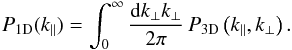 (1)If
all the relevant scales could be treated with in the limit of linear theory, the 3D power
spectrum should be simply related to the mass power spectrum according to
(1)If
all the relevant scales could be treated with in the limit of linear theory, the 3D power
spectrum should be simply related to the mass power spectrum according to
 , where
 , and
bδ and β are the density
bias and redshift distortion parameters of the Lyα forest (McDonald 2003; Slosar et
al. 2011). However, linear theory is valid only on large scales, and even though
the linear expression is valid for P3D when k
is small, the 1D P1D is affected by the non-linearities of small
scales even for very low values of k∥ in Eq. (1). The theoretical interpretation of
measurements of P1D is therefore always dependent on the
nonlinear physics of the intergalactic medium on small scales.
, and
bδ and β are the density
bias and redshift distortion parameters of the Lyα forest (McDonald 2003; Slosar et
al. 2011). However, linear theory is valid only on large scales, and even though
the linear expression is valid for P3D when k
is small, the 1D P1D is affected by the non-linearities of small
scales even for very low values of k∥ in Eq. (1). The theoretical interpretation of
measurements of P1D is therefore always dependent on the
nonlinear physics of the intergalactic medium on small scales.
In the present paper, we measure the 1D transmission power spectrum of the Lyα forest from a sample of 13 821 quasar spectra, which are selected as the highest quality spectra among the set of 61 931 quasars at z > 2.15 from the DR9 quasar catalog of Pâris et al. (2012).
Historically, two approaches have been used to measure the 1D power spectrum of the fluctuations in the transmitted flux fraction F. The first is done directly in Fourier space by computing the FT of δ = F/ ⟨F⟩ − 1 for each quasar spectrum and obtaining the power spectrum from these Fourier modes, as in Croft et al. (1998, 2002) and Viel et al. (2004). The second approach uses a likelihood method to compute the covariance matrix of δ in real space (or line-of-sight correlation function) as a function of the pixel pair separation in the spectra (McDonald et al. 2006). The 1D power spectrum is the FT of the Lyα correlation function obtained in this way. The two methods have their own advantages and drawbacks in terms of, for example, robustness, processing speed, accounting of instrumental effects, precision, etc. To benefit from their complementarity, we have developed independent analysis pipelines based on either technique. In this paper we present and compare the results obtained with the two approaches.
The outline of our paper is as follows. In Sect. 2, we present the BOSS data and explain how we calibrate the level of noise in the spectra and determine the spectrograph resolution. The selection of the quasar spectra and the different steps of the data preparation are presented in Sect. 3. In Sect. 4, we describe the two complementary methods we have developed to analyze the data. We present in Sect. 5 our estimates of the systematic uncertainties associated with each method or due to our imperfect knowledge of the instrument performances. The final results are given in Sect. 6, and a preliminary cosmological interpretation is presented in Sect. 7, along with a comparison to previously published constraints. Conclusions and perspectives are presented in Sect. 8.
2. Data calibration
2.1. BOSS survey
The Sloan Digital Sky Survey (York et al. 2000) mapped over one quarter of the sky using the dedicated 2.5-m Sloan Telescope (Gunn et al. 2006) located at Apache Point Observatory in New Mexico. A mosaic CCD camera (Gunn et al. 1998) used in drift-scanning mode imaged this area in five photometric bandpasses (Fukugita et al. 1996; Smith et al. 2002; Doi et al. 2010) to a limiting magnitude of g ≃ 22.8. The imaging data were processed through a series of pipelines (Stoughton et al. 2002) that performed astrometric calibration, photometric reduction, and photometric calibration. The magnitudes were corrected for Galactic extinction using the maps of Schlegel et al. (1998). As part of the SDSS-III survey (Eisenstein et al. 2011), BOSS imaged an additional 3000 square degrees of sky over that of SDSS-II (Abazajian et al. 2009) in the southern Galactic sky and in a manner identical to the original SDSS imaging. This increased the total imaging SDSS footprint to 14 055 square degrees, with 7600 square degrees at Galactic latitude | b| > 20° in the northern Galactic cap and 3000 square degrees at | b| > 20° in the southern Galactic cap. All of the imaging was reprocessed and released as part of SDSS Data Release 8 (Aihara et al. 2011).
BOSS is a spectroscopic survey primarily designed to obtain spectra and redshifts over a footprint covering 10 000 square degrees for 1.35 million galaxies, 160 000 quasars, and approximately 100 000 ancillary targets. The quasars, whose spectra cover the Lyα forest of interest for this work, are selected with several algorithms based on the SDSS imaging (Yèche et al. 2010; Kirkpatrick et al. 2011; Bovy et al. 2011; Palanque-Delabrouille et al. 2011), which are all summarized in Ross et al. (2012). A full description of the BOSS survey design is given in Dawson et al. (2013). Aluminum plates are drilled with 1000 holes whose positions correspond to the positions of the targets on the focal plane of the telescope. They are manually plugged with optical fibers that feed a pair of double spectrographs. The double-armed BOSS spectrographs are significantly upgraded from those used by SDSS-I/II, covering the wavelength range 3600 Å to 10 000 Å with a resolving power of 1500 to 2600 (Smee et al. 2013). In addition to expanding the wavelength coverage relative to the previous 3850–9200 Å range of SDSS-I, the throughputs have been increased with new CCDs, gratings, and improved optical elements, and the 640-fiber cartridges with 3′′ apertures have been replaced with 1000-fiber cartridges with 2′′ apertures. Each observation is performed in a series of 900-s exposures, integrating until a minimum S/N is achieved for the faint galaxy targets.
2.2. BOSS reduction pipeline
The data are reduced using a pipeline adapted for BOSS from the SDSS-II spectroscopic reduction pipeline (Bolton et al. 2012). All the spectra are wavelength-calibrated, sky-subtracted, and flux-calibrated. The final spectrum for a given object is produced by the coaddition of typically four to seven 900-s individual exposures that can be distributed over several nights of observations. The coadded spectrum is rebinned onto a uniform baseline of Δlog 10(λ) = 10-4 per pixel. The pipeline computes a statistical error estimate for each pixel, incorporating photon noise, CCD read-out noise, and sky-subtraction errors.
For each spectrum, the pipeline also provides a spectral classification and a redshift for the extragalactic objects. A visual inspection is then performed on the spectra of all quasar targets to provide the final classification and redshifts (Pâris et al. 2012).
At low redshift (z < 2.5), the 1D power spectrum has a significant contribution from photon noise, so it is quite sensitive to the precision with which the noise level in the data is known. The spectrograph wavelength resolution is also a major issue on small scales (i.e., large k-modes) where it abruptly reduces the power spectrum by a factor of ~2 at k = 0.01km s-1 and by a factor of 5–10 at k = 0.02km s-1. The accuracy with which noise and spectrograph resolution are determined in the automated pipeline is insufficient for the purpose of this analysis. We have therefore developed techniques to derive corrections, described in the following sections. These refinements were not necessary for measuring the large-scale 3D Lyα correlation function (Busca et al. 2013; Slosar et al. 2013) since the BAO feature occurs on much larger scales than the size of the resolution element, and the noise in the data only affects the amplitude of the power spectrum and not the correlation function where the BAO peak is seen. Instead, we here aim at measuring the absolute level of the power spectrum, which is directly affected by the level of noise, down to scales of a few Mpc, i.e., of a few pixels, where an accurate knowledge of the spectrograph resolution is crucial.
2.3. Calibration of pixel noise
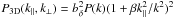
The noise provided by the SDSS-III pipeline is known to suffer from systematic underestimates e.g., (McDonald et al. 2006; Desjacques et al. 2007). To investigate the extent of this issue, we examined the pixel variance in spectral regions that are intrinsically smooth and flat. We used two 50 Å regions of quasar spectra (hereafter “side-bands”), redwards of the Lyα peak: 1330 < λRF < 1380 Å and 1450 < λRF < 1500 Å. These bands are not affected by Lyα forest absorption and have a quasar unabsorbed flux that is relatively flat with wavelength. For each individual quasar, we computed the ratio of the mean pipeline error estimate in the band, ⟨σp⟩, to the root-mean-square (rms) of the pixel-to-pixel flux dispersion within the same band. This quantity is averaged over all DR9 quasars, giving us a wavelength-dependent measure of the accuracy of the pipeline noise estimate because of the distribution of quasar redshifts (see Fig. 1). For a perfect noise estimation, the plotted quantity should be unity at all wavelengths; on the other hand, under (over) estimates will produce values below (above) unity. The flux dispersion in the blue part of the spectra (λ < 4000 Å) is seen to be about 15% larger than expected from the noise level given by the pipeline. The discrepancy decreases with increasing wavelength, and the two estimates are in agreement at λ ≃ 5700 Å.
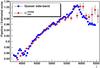 |
Fig. 1 Ratio of the pipeline noise estimate to the actual flux dispersion in the spectra. The blue squares denote this ratio as estimated from the quasar 1330 < λRF < 1380 Å and 1450 < λRF < 1500 Å sidebands. The red points indicate the correction from our procedure (Eq. (2)) as a function of mean forest wavelength. |
This test clearly indicates a wavelength-dependent miscalibration of the noise. However, since some of the flux dispersion in the quasar sidebands can arise from intervening metals along the sightline (see correction of the metal contribution to the power spectrum in Sect. 6.1), this procedure could overestimate the true noise. In Lee et al. (2013), we provided a per-quasar correction to the pipeline noise that was sufficient for BAO studies, but still not accurate enough for this power-spectrum analysis. Here, we recalibrate the pixel noise for each quasar as described below. This new correction deviates from the one described in Lee et al. (2013) at most by a few percent.
We made use of the typically four to seven individual exposures that contribute to a
given quasar spectrum and split them into two interleaved sets: one containing the odd and
the other the even exposures. For each set, we computed the weighted average spectrum with
weights equal to the pixel inverse variance  given by the pipeline of BOSS, binned into pixels of width
Δlog 10(λ) = 10-4 as for the final coadded
spectrum. We then computed a “difference spectrum” Δφ by subtracting the
spectrum obtained for one set from the one for the other set. In this process, we mask all
pixels affected by sky emission lines (cf. Sect. 5.1) by setting to 0 the value of the corresponding pixel in the difference
spectrum. The difference spectrum should have all physical signal removed and only contain
signal fluctuations. It can therefore be used to directly determine the level of noise in
the data, irrespective of any miscalibration of the pixel noise in the reduction pipeline.
This procedure also has the advantage of evaluating the noise level for each individual
spectrum and not on a statistical basis.
given by the pipeline of BOSS, binned into pixels of width
Δlog 10(λ) = 10-4 as for the final coadded
spectrum. We then computed a “difference spectrum” Δφ by subtracting the
spectrum obtained for one set from the one for the other set. In this process, we mask all
pixels affected by sky emission lines (cf. Sect. 5.1) by setting to 0 the value of the corresponding pixel in the difference
spectrum. The difference spectrum should have all physical signal removed and only contain
signal fluctuations. It can therefore be used to directly determine the level of noise in
the data, irrespective of any miscalibration of the pixel noise in the reduction pipeline.
This procedure also has the advantage of evaluating the noise level for each individual
spectrum and not on a statistical basis.
We computed the quantity  , where
ℱ(Δφ) is the FT of the difference spectrum Δφ. In Fig.
2, we plot the average of
, where
ℱ(Δφ) is the FT of the difference spectrum Δφ. In Fig.
2, we plot the average of
 computed over
the Lyα forest of quasars, for three ranges in Lyα
redshifts (or equivalently three ranges in observed wavelength). The noise is expected to
be white, and is indeed seen
to be scale-independent to an accuracy sufficient for our purposes. For comparison, we
also show in the figure the power spectrum of coadded spectra where both signal and noise
are present. The noise power spectrum approaches the same order of magnitude as the raw
power spectrum on small scales (k ~ 0.02km s-1) and low
redshifts (z < 2.4). This is therefore the region
where it is most important to accurately determine its contribution.
computed over
the Lyα forest of quasars, for three ranges in Lyα
redshifts (or equivalently three ranges in observed wavelength). The noise is expected to
be white, and is indeed seen
to be scale-independent to an accuracy sufficient for our purposes. For comparison, we
also show in the figure the power spectrum of coadded spectra where both signal and noise
are present. The noise power spectrum approaches the same order of magnitude as the raw
power spectrum on small scales (k ~ 0.02km s-1) and low
redshifts (z < 2.4). This is therefore the region
where it is most important to accurately determine its contribution.
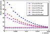 |
Fig. 2 Average power spectra of the raw (filled dots) and of the difference (open circles) signal for three ranges in Lyα redshifts. |
We derived the “pipeline noise power spectrum”  from the error
σp given by the pipeline in each pixel.
would be the
true noise power spectrum if the pipeline error estimate were correct. For each individual
quasar, we thus derive a correction coefficient of the pixel flux error as
from the error
σp given by the pipeline in each pixel.
would be the
true noise power spectrum if the pipeline error estimate were correct. For each individual
quasar, we thus derive a correction coefficient of the pixel flux error as  (2)where
the power spectra are computed in both cases over the pixels in the quasar forest and
averaged over k. In Fig. 1, the
value of the correction term is shown, averaged over all the DR9 quasars; as before, the
distribution of quasar redshifts provides a wavelength-dependent measurement. We observe,
on average, excellent agreement between
(2)where
the power spectra are computed in both cases over the pixels in the quasar forest and
averaged over k. In Fig. 1, the
value of the correction term is shown, averaged over all the DR9 quasars; as before, the
distribution of quasar redshifts provides a wavelength-dependent measurement. We observe,
on average, excellent agreement between  and the
noise miscalibration estimated in quasar sidebands. In the latter case, however, the
estimate is derived from lower redshift quasars whose sideband covers the same wavelength
region as the Lyα forest of higher redshift quasars. The method based on
spectrum differences, in contrast, uses the forest data directly and is thus a better
estimate of the noise in each quasar spectrum. For each quasar, the corrected pixel error
σ is derived from the pipeline pixel error
σp by
and the
noise miscalibration estimated in quasar sidebands. In the latter case, however, the
estimate is derived from lower redshift quasars whose sideband covers the same wavelength
region as the Lyα forest of higher redshift quasars. The method based on
spectrum differences, in contrast, uses the forest data directly and is thus a better
estimate of the noise in each quasar spectrum. For each quasar, the corrected pixel error
σ is derived from the pipeline pixel error
σp by 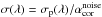 .
.
2.4. Calibration of spectrograph resolution
For each co-added spectrum, the spectral resolution is provided by the BOSS reduction pipeline (Bolton et al. 2012). Since the measurement of the 1D power spectrum on small scales is extremely sensitive to the spectrograph resolution, we first investigated the resolution given by the pipeline and we determined a correction table.
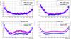 |
Fig. 3 Comparison of the resolution given by the pipeline (blue circles) and our computation (purple crosses) for arc lamp or sky line as a function of fiber number (i.e. position of spectrum on CCD). Upper left: comparison with arc lamp for a mercury line at ~3650 Å. Upper right: comparison with arc lamp for a cadmium line at ~4800 Å. Lower left: comparison with arc lamp for a mercury line at ~5461 Å. Lower right: comparison with the OI sky line at ~5577 Å. |
2.4.1. Spectrograph resolution in the BOSS pipeline
In BOSS, spectral lamps are used to provide the wavelength calibration, as described in Smee et al. (2013). In the present work, we are mostly interested in the calibration of the blue CCD, which is obtained from its illumination with a mercury-cadmium arc lamp (with seven principal emission lines in the blue and the green parts of the spectrum).
The spectral resolution is measured from calibration arc lamp images taken before each set of science exposures. The pipeline procedure fits a Gaussian distribution around the position of the mercury and cadmium lines. The mean mλ and the width σλ of the Gaussian determine the absolute wavelength on the CCD and the resolution of the spectrograph, respectively. A fourth-order Legendre polynomial is fit to the derived σλ as a function of wavelength to model the dispersion over the full wavelength range.
2.4.2. Precision of pipeline resolution
The BOSS reduction pipeline provides the spectrograph resolution σλ,i for each pixel i of each spectrum. On a set of plates, we performed our own Gaussian fits on the mercury and cadmium lines, and we compared our measurement to the resolution given by the BOSS pipeline. We observe systematic shifts that depend on two parameters: wavelength (given by the emission wavelength of the line), and position of the spectrum on the CCD (given by the fiber number). Each CCD has 500 fibers, with numbers 1 and 500 corresponding to CCD edges while numbers near 250 correspond to the central region of the CCD. This comparison is illustrated as a function of fiber number with the first three plots of Fig. 3, corresponding to three lines of mercury and cadmium. The disagreement is at most of a few percent. It is greater in the central region of the CCD and less on the edges. The disagreement increases with wavelength and reaches 10% on the blue CCD, near λ = 6000 Å.
We also checked the wavelength calibration using the brightest sky line observed on the blue CCD: the OI line at ~5577 Å. The comparison between the BOSS pipeline and our computation of the resolution (see fourth plot of Fig. 3) shows a similar discrepancy as that observed directly with the mercury arc lamp for similar wavelengths.
2.4.3. Correction of pipeline resolution
In our analysis, we start from the resolution given by the BOSS reduction pipeline, to which we apply a correction to take the discrepancy into account that we observe between the pipeline resolution and our estimate, whether with the arc lamp or a skyline. The top plot of Fig. 4 shows the correction as a function of wavelength for spectra in the central region of the CCD. The amplitude of this correction is small, on the order of 10% in the worst case (central spectra and large wavelength for the blue CCD). The bottom plot of Fig. 4 shows the 2D correction to the resolution that we apply in our analysis, as a function of wavelength (second-order polynomial) and fiber number (bounded first-order polynomial).
 |
Fig. 4 Top: correction of the pipeline resolution for spectra in the middle of the CCD (fiber numbers ~250). The curve is the best second-order polynomial fit to the measurements at the arc-lamp wavelengths. Bottom: 2D correction table of the pipeline resolution as a function of fiber number (ie. position of spectrum on CCD) and wavelength. |
3. Quasar selection and data preparation
3.1. Data selection
We define the Lyα forest by the range 1050 < λRF < 1180 Å, thus at least 7000 km s-1 away from the quasar Lyβ and Lyα emission peaks. We limit the spectra to wavelengths above the detector cutoff, i.e., to λ > 3650 Å, corresponding to an absorber redshift of z = 2.0.
The Lyα forest spans a redshift range Δz ~ 0.4 for a quasar at a redshift zqso = 2.5, and Δz ~ 0.6 for a quasar redshift zqso = 5.0. To improve our redshift resolution to Δz < 0.2 without overly affecting the k-resolution and at the same time, to reduce the computation time for the likelihood approach (details in the analysis part, Sect. 4), we split the Lyα forest into two or three (depending on the length of the Lyα forest) consecutive and non-overlapping subregions of equal length, hereafter called “z-sectors”. A non-truncated Lyα forest contains 507 pixels and is divided into three z-sectors of 169 pixels each. At low redshift (zqso < 2.5) the forest extension is limited by the CCD UV cutoff. In practice, the forest is divided into three z-sectors down to a forest length of 180 pixels, into two z-sectors for a forest length between 90 and 180 pixels and not subdivided otherwise. This procedure ensures that the redshift range spanned by a z-sector is at most 0.2.
With a pixel size Δv = cΔλ/λ = 69km s-1, the smallest k-mode is therefore between kmin = 5 × 10⁻⁴ km s-1 and kmin = 10-3 km s-1 depending on the actual z-sector length. Our largest possible mode is determined by the Nyquist-Shannon limit at kNyquist = π/Δv = 4.5 × 10⁻² km s-1, but we limit our analysis to kmax = 0.02km s-1 because of the large window function correction (mostly due to the spectrograph resolution, cf. Fig. 10) for modes of larger k.
We used the quasars from the DR9 quasar catalog of BOSS (Pâris et al. 2012). The full catalog contains 61 931 quasars, of which we
selected the best 13 821 on the basis of their mean S/N in the Lyα
forest, spectrograph resolution ( ), and
quality flags on the pixels. Flags were also set during the visual scanning of the
spectra. We rejected all quasars that have broad absorption line features (BAL), damped
Lyman alpha (DLA) or detectable Lyman limit systems (LLS) in their forest.
), and
quality flags on the pixels. Flags were also set during the visual scanning of the
spectra. We rejected all quasars that have broad absorption line features (BAL), damped
Lyman alpha (DLA) or detectable Lyman limit systems (LLS) in their forest.
The total noise per pixel decreases on average with wavelength by about a factor of 2
between 3650 and 4000 Å and by another factor of 2 between 4000 and 6000 Å. We reject
quasars with
S/N < 2,
where the S/N is averaged over the Lyα forest. This criterion mostly
removes low-redshift quasars, since they have their Lyα forest in the
blue, hence noisiest, part of the spectrograph. The spectrograph resolution
R varies slightly with wavelength, from typically
~82 km s-1 (at 1σ) at 3650 Å to
~61 km s-1 at 6000 Å. It also varies with the position of the spectrum on
the CCD (cf. Fig. 3), with a resolution in the
central part that is about 7 km s-1 lower than in the outer regions. We reject
quasars with a resolution, averaged over the Lyα forest,
 to limit the effect of the velocity resolution in the derived power spectrum. We also
remove quasars with pixels in their Lyα forest that are masked by the
pipeline (<2% of the sample). The purpose of these restrictions is
to ensure that the systematic uncertainty coming from the precision with which the
spectrograph noise and resolution can be calibrated remains less than the statistical
uncertainty of the estimated power spectra. These uncertainties will be explained in Sect.
5.2. Because both the noise and the resolution are
worse in the blue part of the spectrograph, these cuts affect the low-redshift more than
the high-redshift quasars. Since the former are also much more numerous, we can thus
improve the quality of our sample in a region where the systematic uncertainties would
otherwise dominate the statistical ones.
to limit the effect of the velocity resolution in the derived power spectrum. We also
remove quasars with pixels in their Lyα forest that are masked by the
pipeline (<2% of the sample). The purpose of these restrictions is
to ensure that the systematic uncertainty coming from the precision with which the
spectrograph noise and resolution can be calibrated remains less than the statistical
uncertainty of the estimated power spectra. These uncertainties will be explained in Sect.
5.2. Because both the noise and the resolution are
worse in the blue part of the spectrograph, these cuts affect the low-redshift more than
the high-redshift quasars. Since the former are also much more numerous, we can thus
improve the quality of our sample in a region where the systematic uncertainties would
otherwise dominate the statistical ones.
Table 1 summarizes the impact of our cuts on the quasar sample. Figure 5 shows the distributions of the quasar redshifts and of the z-sector mean redshifts for the quasars and z-sectors that pass these criteria.
Summary of main quasar selection cuts and fraction of quasars passing previous cuts rejected at each step.
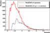 |
Fig. 5 Redshift distribution of the 13 821 quasars selected in the analysis, and mean redshift distribution of each z-sector of their Lyα forest. |
In Fig. 6, we show average quasar spectra obtained by averaging the spectra of all the DR9 BOSS quasars passing the above cuts, split into five redshift bins from z = 2.3 to 4.3. Broad quasar emission lines are clearly visible, such as Lyβ at λRF ~ 1026 Å, Lyα at λRF ~ 1216 Å, N v at λRF ~ 1240 Å, Si iv at λRF ~ 1400 Å and C iv at λRF ~ 1549 Å. The absorption by Lyα absorbers along the quasar line of sight appears blueward of the quasar Lyα emission peak, with more absorption (and thus less transmitted flux) at high redshift.
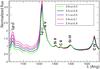 |
Fig. 6 Average quasar spectra in five redshift bins. All spectra are normalized at λ = 1280 Å. |
We calculate the 1D power spectra in twelve redshift bins of width Δz = 0.2 and centered on zc = 2.2 to zc = 4.4. The mean redshift of the Lyα absorbers of a given z-sector determines the redshift bin to which it contributes. While the Lyα forest of a quasar spectrum may cover several redshift bins, a given z-sector only contributes to a single bin, thus avoiding correlations between redshift bins. The redshift span of a z-sector, at most 0.2, is adapted well to the size of our redshift bins.
3.2. Sky line masking
Sky lines affect the data quality by increasing significantly the pixel noise. The procedure used to identify them is detailed in Lee et al. (2013). We briefly summarize it here.
We use the sky calibration fibers and compute the mean and the rms of the residuals measured on the sky-subtracted spectrum obtained with the standard BOSS pipeline. We define a “sky continuum” as the running average of the residual rms fluctuation centered on a ± 25 pixel window, and generate a list of sky lines from all the wavelengths that are above 1.25 × the sky continuum. The continuum, measured with the unmasked pixels, and the sky line list are iterated until they converge. To this list, we add the calcium H and K Galactic absorption lines near λ = 3933.7 Å and λ = 3968.5 Å. We then mask all pixels that are within 1.5 Å of the listed wavelengths.
We apply the mask differently in the FT and the likelihood methods. For the FT, we replace the flux of each masked pixel by the average value of the flux over the unmasked forest. This procedure introduces a k-dependent bias in the resulting power spectrum that reaches at most 15% at small k for the 3.5 < z < 3.7 redshift bin, which contains 5577 Å OI, the strongest sky emission line. We correct for this bias a posteriori, as explained in Sect. 5.1. For the likelihood method, the masked pixels are simply omitted from the data vector. We have checked (see details in Sect. 5.1) that in this case we observe no bias on the resulting power spectrum.
3.3. Quasar continuum
The normalized transmitted flux fraction δ(λ) is
estimated from the pixel flux f(λ) by: 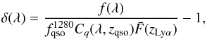 (3)where
 is a
normalization equal to the mean flux in a 20 Å window about
λRF = 1280 Å,
Cq(λ,zqso)
is the normalized unabsorbed flux (the mean quasar “continuum”) and
is a
normalization equal to the mean flux in a 20 Å window about
λRF = 1280 Å,
Cq(λ,zqso)
is the normalized unabsorbed flux (the mean quasar “continuum”) and
 is the mean transmitted flux fraction at the H i absorber redshift. Pixels
affected by sky line emission are not included when computing the normalization. Since the
mean quasar continuum is flat in the normalization region, the rejection of a few pixels
does not bias the mean pixel value. The product
is the mean transmitted flux fraction at the H i absorber redshift. Pixels
affected by sky line emission are not included when computing the normalization. Since the
mean quasar continuum is flat in the normalization region, the rejection of a few pixels
does not bias the mean pixel value. The product  is assumed to be universal for all quasars at redshift zqso
and is computed by stacking appropriately normalized quasar spectra
is assumed to be universal for all quasars at redshift zqso
and is computed by stacking appropriately normalized quasar spectra
 , thus
averaging out the fluctuating Lyα absorption. The product
, thus
averaging out the fluctuating Lyα absorption. The product
 represents the mean expected
flux, and the transmitted flux fraction is given by
represents the mean expected
flux, and the transmitted flux fraction is given by
 . For a
pixel at rest-frame wavelength λRF of a quasar at redshift
zqso, the corresponding H i absorber redshift
zLyα can be inferred from
1 + zLyα = λRF/λLyα × (1 + zqso),
where λLyα ≃ 1216 Å.
. For a
pixel at rest-frame wavelength λRF of a quasar at redshift
zqso, the corresponding H i absorber redshift
zLyα can be inferred from
1 + zLyα = λRF/λLyα × (1 + zqso),
where λLyα ≃ 1216 Å.
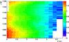 |
Fig. 7 Product of the quasar continuum
Cq(λ,zqso)
by the mean transmitted flux fraction |
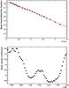 |
Fig. 8 Top: mean transmitted fraction
|
Figure 7 shows the product
 of the quasar continuum with the mean transmitted flux fraction as a function of
rest-frame wavelength and Lyα redshift. Figure 8 shows the projection of the 2D distribution of Fig. 7 onto the redshift or the wavelength axis. The former
shows
of the quasar continuum with the mean transmitted flux fraction as a function of
rest-frame wavelength and Lyα redshift. Figure 8 shows the projection of the 2D distribution of Fig. 7 onto the redshift or the wavelength axis. The former
shows  averaged over wavelength and is proportional to the mean transmitted flux fraction, and
the latter shows the mean unabsorbed quasar spectrum
Cq(λ) normalized to
. The
mean transmitted flux fraction is well fit by a function of the form
exp [−α(1 + z)β], with
α ~ 0.0046 and β ~ 3.3, in agreement with previous
measurements of the optical depth τeff where
averaged over wavelength and is proportional to the mean transmitted flux fraction, and
the latter shows the mean unabsorbed quasar spectrum
Cq(λ) normalized to
. The
mean transmitted flux fraction is well fit by a function of the form
exp [−α(1 + z)β], with
α ~ 0.0046 and β ~ 3.3, in agreement with previous
measurements of the optical depth τeff where
 (see e.g. Meiksin 2009, for a review).
The values in the 2D table, ,
differ from those of the product  by up to 5%, possibly due to variations in the mean quasar continuum with redshift.
Despite its lower statistical precision for a given wavelength and redshift, we therefore
use the 2D table.
by up to 5%, possibly due to variations in the mean quasar continuum with redshift.
Despite its lower statistical precision for a given wavelength and redshift, we therefore
use the 2D table.
Figure 9 shows the resulting mean δ as a function of observed wavelength. The mean fluctuates about zero at the 2% level with correlated features that are due to imperfect spectrograph calibration and absorption. These features include the calcium H-K doublet at (3934, 3968 Å) from Milky Way absorption, and Balmer lines Hγ, δ, ϵ at (4341, 4102, 3970 Å) that are residuals from the use of F-stars as spectrocalibration standards. Busca et al. (2013) have studied these features in detail and concluded that they had quasar-to-quasar variations of less than 20% of the mean Balmer artifact deviations. To remove their contribution to the Lyα power spectrum, we subtract the mean residual of Fig. 9 from δ(λ).
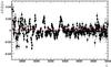 |
Fig. 9 Mean of δ(λ) as a function of wavelength in Å. Systematic offsets from zero are seen at the 2% level due to imperfections in the spectrograph calibration. |
4. Methods for determining P(k)
We apply two methods to compute the one-dimensional power spectrum. The first one is based on a FT. It is fast and robust, thus allowing many tests leading to a better understanding of the impact of the different ingredients entering the analysis. We use it to test the impact of, for instance, different selections of quasars on the precision of the resulting power spectra or various algorithms to mask sky emission lines. The second method relies upon a maximum likelihood estimator in real space. It can take variations in the noise or in the spectrograph resolution at the pixel level into account instead of through global factors, and is therefore expected to be more precise than a FT. It also offers a natural way to mask pixels affected by sky emission lines, as explained in Sect. 4.2. However, it is more sensitive than the FT to details in the implementation of the method, is susceptible to convergence problems in the presence of noisy spectra and is more time-consuming. It is therefore not as flexible for algorithm testing. The power spectra obtained with the two approaches are in good agreement. Their comparison provides an estimate of the systematic uncertainty on our measurement (cf. Sect. 6.3).
4.1. Fourier transform approach
4.1.1. Measurement of the power spectrum with a Fourier transform
To measure the 1D power spectrum P1D(k) we decompose each absorption spectrum δΔv into Fourier modes and estimate their variance as a function of wave number. In practice, we do this by computing the discrete FT of the flux transmission fraction δ = F/ ⟨F⟩ −1 as described in Croft et al. (1998), using a fast Fourier transform (FFT) algorithm. Using a FFT requires that the pixels be equally spaced. This condition is satisfied with the quasar coadded spectra provided by the SDSS pipeline (Bolton et al. 2012): the spectra are computed with a constant pixel width Δ [log (λ)] = 10-4, and the velocity difference between pixels, i.e., the relative velocity of absorption systems at wavelengths λ + Δλ/2 and λ − Δλ/2, is Δv = c Δλ/λ = c Δ [ln(λ)]. The coadded spectra thus have equally spaced pixels in Δv. Throughout this paper we therefore use velocity instead of observed wavelength. Similarly, the wave vector k ≡ 2π/Δv is measured in km s-1.
In the absence of instrumental effects (noise and resolution of the spectrograph), the 1D power spectrum can be simply written as the ensemble average over quasar spectra of Praw(k) ≡ |ℱ(δΔv)|2, where ℱ(δΔv) is the FT of the normalized flux transmission fraction δΔv in the quasar Lyα forest binned in pixels of width Δv.
When taking the noise in the data and the impact of the spectral resolution of the
spectrograph into account, δ can be expressed as
δ = s + n, with s
the signal and n the noise, and the estimator of the 1D power spectrum
is 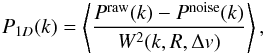 (4)where
⟨ ⟩ denotes the ensemble average over quasar spectra and where
(4)where
⟨ ⟩ denotes the ensemble average over quasar spectra and where
 (5)The
window function corresponding to the spectral response of the spectrograph is defined by
(5)The
window function corresponding to the spectral response of the spectrograph is defined by
 (6)where
Δv and R are the pixel width and the spectrograph
resolution, respectively. Both quantities are in km s-1, and
R should not be confused with the dimensionless resolving power of
the spectrograph. We illustrate in Fig. 10 the
spectrograph resolution on the window function
(6)where
Δv and R are the pixel width and the spectrograph
resolution, respectively. Both quantities are in km s-1, and
R should not be confused with the dimensionless resolving power of
the spectrograph. We illustrate in Fig. 10 the
spectrograph resolution on the window function  for different values of
  .
.
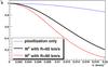 |
Fig. 10 Window function |


4.1.2. Computation of P1D(k) with an FFT
We compute the FT using the efficient FFTW package1. Compared to the likelihood approach described in the next section, the Fourier transform is much faster, but it requires some simplifying hypotheses in the treatment of the noise and of the spectrograph resolution. We explain these simplifications below. Sky emission lines are also treated in a simplified way as described in Sect. 3.2. The results provided by this simple method are complementary to the likelihood approach.
Although the redshift of the absorbing hydrogen increases with wavelength along the spectrum of a given quasar, the power spectrum is considered to be computed at their average redshift. As explained in Sect. 3.1, we improve the redshift resolution of the measured power spectra by splitting the Lyα forest of each quasar into redshift subregions (or z-sectors, see Sect. 3.1). The computation is done separately on each z-sector instead of on the entire Lyα forest. The mean redshift of the Lyα absorbers in the z-sector determines the redshift bin to which the z-sector contributes.
The noise power spectrum Pnoise(k,z) is
taken as the power spectrum on the
z-sector, computed as explained in Sect. 2.3. Since is flat with
k, we improve the statistical precision on our determination of the
level of the noise power spectrum by taking the average of
 for
k < 0.02 km s-1.
for
k < 0.02 km s-1.
Finally, we apply the correction of the spectrograph resolution by dividing by
 ,
where
,
where  is the
mean value of the spectral resolution R averaged over the
z-sector. The value of R is given by the pipeline
and corrected following the prescription described in Sect. 2.4. For a given spectrum, R varies by less than 10%
over the Lyα forest (less than 3% over a z-sector),
and the impact of this simplification is negligible.
is the
mean value of the spectral resolution R averaged over the
z-sector. The value of R is given by the pipeline
and corrected following the prescription described in Sect. 2.4. For a given spectrum, R varies by less than 10%
over the Lyα forest (less than 3% over a z-sector),
and the impact of this simplification is negligible.
We rebin the final power spectrum onto a predefined grid in k-space, giving equal weight to the different Fourier modes that enter each bin. The final 1D power spectrum is obtained by averaging the corrected power spectra of all the contributing z-sectors of all selected quasars, as expressed in Eq. (4).
4.2. Likelihood approach
We estimate P1D(k) using a maximum likelihood estimator derived from methods developed for studies of the cosmic microwave background anisotropy (Bond et al. 1998; Seljak 1998). This method guarantees optimal performance for Gaussian or nearly Gaussian distributions, and can be applied here ensuring minimal variance, although the power spectrum estimates are not Gaussian distributed. Our approach involves a direct maximization of the likelihood function and is not based on the quadratic maximum estimation as in McDonald et al. (2006). It is slower but provides the values of P1D(k) with their covariance matrix at the maximum of the likelihood.
4.2.1. The likelihood function
We model the normalized flux transmission fraction
δi = Fi/ ⟨F⟩ − 1
measured in pixel i as contributions from signal and noise:
δi = si + ni.
We assume that signal and noise are independent, with zero mean and covariance matrices
given by  (7)where
δij is the Kronecker symbol and
(7)where
δij is the Kronecker symbol and
 (pipeline
estimate and its correction). The total covariance matrix can therefore be written as
(pipeline
estimate and its correction). The total covariance matrix can therefore be written as
 (8)The
signal covariance matrix can be derived from the 1D power spectrum by
(8)The
signal covariance matrix can be derived from the 1D power spectrum by
![Mathematical equation: \begin{eqnarray*} C_{ ij}^S & = & \int_{-\infty}^{+\infty}P_{1D}(k)\cdot\exp\left[ -{\rm i}k\Delta v \times (i-j)\right] {\rm d}k \\ & = &\int_{0}^{+\infty}P_{1D}(k)\cdot 2\cos\left[ k\Delta v \times (i-j) \right] \, {\rm d}k . \\ \end{eqnarray*}](/articles/aa/full_html/2013/11/aa22130-13/aa22130-13-eq187.png) We
can approximate P1D by
P = (P1,...Pℓ...,PNℓ),
a discrete set of Nℓ values of
We
can approximate P1D by
P = (P1,...Pℓ...,PNℓ),
a discrete set of Nℓ values of
 for the modes kℓ. The previous integral can
then be approximated by
for the modes kℓ. The previous integral can
then be approximated by ![Mathematical equation: \begin{eqnarray} C_{ ij}^S(\boldsymbol{P} ) & = & \sum_{\ell=1}^{N_\ell} P_\ell \cdot \int_{k_{\ell-1}}^{k_\ell} 2\cos\left[ k\Delta v\times (i-j)\right] \, {\rm d}k . \end{eqnarray}](/articles/aa/full_html/2013/11/aa22130-13/aa22130-13-eq193.png) (9)Taking
the spectrograph resolution into account and using the definition of the window function
given in Eq. (6), the covariance matrix
becomes
(9)Taking
the spectrograph resolution into account and using the definition of the window function
given in Eq. (6), the covariance matrix
becomes ![Mathematical equation: \begin{eqnarray*} C_{ ij}^S(\boldsymbol{P} ) &=& \sum_{\ell=1}^{N_\ell} P_\ell \cdot \int_{k_{\ell-1}}^{k_\ell} 2 \cos\left[ k \Delta v\times (i-j)\right] \\ & & \times~W(k,R_i,\Delta v) W(k,R_j,\Delta v)\, {\rm d}k \end{eqnarray*}](/articles/aa/full_html/2013/11/aa22130-13/aa22130-13-eq194.png) where
Ri and Δv are
respectively the spectrograph resolution for pixel i and the pixel
width (same for all pixels).
where
Ri and Δv are
respectively the spectrograph resolution for pixel i and the pixel
width (same for all pixels).
For spectrum sp containing  pixels, we can
define the likelihood function ℒsp as
pixels, we can
define the likelihood function ℒsp as
 (10)For
stability reasons, we do not fit a single spectrum at a time but instead combine
Nsp spectra corresponding to the same redshift bin into a
common likelihood. The likelihood is the product:
(10)For
stability reasons, we do not fit a single spectrum at a time but instead combine
Nsp spectra corresponding to the same redshift bin into a
common likelihood. The likelihood is the product:  (11)We
can then search for the vector P(z) (i.e.
the parameters Pℓ(z)) that
maximizes this likelihood.
(11)We
can then search for the vector P(z) (i.e.
the parameters Pℓ(z)) that
maximizes this likelihood.
4.2.2. Extraction of P1D(k)
We extract the P1D(k) power spectrum from the likelihood ℒ(P(z)) that combines several spectra in the same redshift bin. We use the MINUIT (James & Ross 1975) package to minimize the term −2ln(ℒ). This minimization provides the value and the error of each Pℓ(z) and the covariance matrix between the different Pℓ(z). The method implemented in MINUIT package may be slow but it is robust, because it seldom falls into secondary minima.
As the minimization can take a few hundred iterations, we have optimized our fitting procedure. The computation time of the likelihood is limited by the inversion of the covariance matrix C. Therefore, to reduce the size of the matrix C (number of pixels), we do the computation on the “z-sectors” defined in Sect. 3.1, instead of on the entire Lyα forest.
The noise covariance matrix is assumed diagonal, i.e., without correlation terms. Each
diagonal element is equal to the square of the pixel error estimated by the pipeline,
σp, multiplied by the square of the
correction factor defined in
Eq. (2).
We use the Cholesky decomposition to increase the speed of the matrix inversion of the positive-definite matrix C. The Cholesky decomposition is roughly twice as efficient as the LU decomposition, and it is numerically more precise.
Finally, in the product of the individual likelihoods of Eq. (11), we take
Nsp = 100 where in practice Nsp
is the number of z-sectors and not the number of quasar spectra. While
a large Nsp improves the fit convergence by making the fit
more stable, we nevertheless restrict the number of z-sectors to be
fitted simultaneously in order to limit the minimization to a reasonable CPU time. We
determine the final P(z) by averaging
over the Nb bunches of
Nspz-sectors (with
Nb × Nsp being the total
number of z-sectors that enter a given redshift bin). The total
covariance matrix  is computed as
 .
.
The typical CPU time for the minimization of one bunch of 100 z-sectors is about 10 to 15 min, performing between 500 and 600 iterations before convergence. For this analysis, we ran on a farm of 24 computers, which allowed us to compute the independent power spectra for different redshift bins in parallel. The total wall-clock time for the full analysis is approximately 12 h.
5. Systematic uncertainties
In this section, we study the biases and systematic uncertainties that affect our analysis. We correct our result for the identified biases, and we estimate systematic uncertainties that we summarize in Sect. 6 (Tables 4 and 5), along with our measured power spectrum.
The biases and uncertainties arise from two different origins. In Sect. 5.1, the biases related to the analysis methods, either FT or likelihood, are presented assuming that the instrumental noise and resolution are perfectly known. Then in Sect. 5.2, the systematics due to our imperfect knowledge of the instrument characteristics are described and quantified using the data themselves.
5.1. Biases in the analyses and related systematics
We study here the biases and systematic uncertainties introduced at each step of the data analysis. We estimate their impact using mock spectra. We compute the “bias” of the method as the ratio of the measured flux power spectrum to the flux power spectrum that was generated in the mock spectra.
We generated mock spectra with the following procedure. First, a redshift and a g-magnitude are chosen at random from the real BOSS spectra. Second, an unabsorbed flux spectrum is drawn for each quasar from a random selection of PCA amplitudes following the procedure of Pâris et al. (2011) and flux-normalized to the selected g magnitude. Third, the Lyα forest absorption is generated following a procedure adapted from Font-Ribera et al. (2012). They provide an algorithm for generating any spectrum of the transmitted flux fraction F(λ) from a Gaussian random field g(λ). Specifically, they present a recipe for choosing the parameters a and b and the power spectrum Pg(k) such that the transformation F(λ) = exp [−aexp (bg(λ))] yields the desired power spectrum and mean value of F(λ). In practice we generate a suite of transmitted-flux-fraction spectra for twelve redshifts that reproduce the observed power. For each wavelength pixel, F(λ) is obtained by interpolation between redshifts according to the actual Lyα absorption redshift of the pixel. The unabsorbed flux is multiplied by F(λ) and convolved with the spectrograph resolution. In practice, the spectra are generated with a pixel width that is one third of an SDSS pixel, and about one third of the spectral resolution. We checked that this size was small enough to take the spectral resolution into account properly. Finally, noise is added according to BOSS throughput and sky noise measurements as was done in Le Goff et al. (2011), and the spectrum is rebinned to the SDSS bin size.
The determination of the transmitted flux fraction requires an estimate of the quasar
unabsorbed flux obtained as explained in Eq. (3) of Sect. 3.3. As a starting point, we
have checked that using the generated values for the quasar continuum
Cq(λ) and for the mean
transmitted flux  allows recovery of exactly the input power spectra in the absence of noise. Using instead
our estimated value of
allows recovery of exactly the input power spectra in the absence of noise. Using instead
our estimated value of  produces an overestimate of the power spectrum of order 2%, and is
k-independent over the k-range of interest. To have a
better estimate of the continuum on a quasar-by-quasar basis and allow for tilts in the
flux calibration, we considered an improved method consisting of multiplying the average
shape by a factor A + BλRF
where A and B were fitted for each quasar. This method
was not retained, however, because it generated a larger overestimate (~6%).
produces an overestimate of the power spectrum of order 2%, and is
k-independent over the k-range of interest. To have a
better estimate of the continuum on a quasar-by-quasar basis and allow for tilts in the
flux calibration, we considered an improved method consisting of multiplying the average
shape by a factor A + BλRF
where A and B were fitted for each quasar. This method
was not retained, however, because it generated a larger overestimate (~6%).
We studied the impact of our correction for the spectrograph spectral resolution W(k,R,Δv) by using mocks where W was either similar to that of BOSS (including both pixellization and spectrograph resolution) or reduced to the contribution of pixellization alone (cf. Fig. 10). We found negligible bias (less than 0.1%) in both the FT and the likelihood methods.
The removal of the noise contribution to the Lyα power spectrum introduces a bias in both methods. For mock spectra, the noise power spectrum is white, and we determine its level directly from the pixel errors. For the FT approach, the removal of the noise power spectrum on mock spectra analyzed with the true quasar continuum produces a small (2%) underestimate.
The likelihood method is much more sensitive than the Fourier transform approach to the level of noise and to the relative levels of noise and signal power spectra. It results in biases that can reach ~13% at low redshift (z < 2.3) and on small scales (k > 0.015), where noise is high and signal is low (cf. Fig. 2). The cause of this bias has not been identified. To correct for it, we produced mock spectra covering the range in Pnoise and Praw observed in the data. While the noise is white, the k-dependence of Praw provides a wide range of relative values of Pnoise and Praw with each power spectrum. We measured a systematic overestimate of the power spectrum (cf. Fig. 11), which we modeled by c0 + c1 × Pnoise/Praw + c2 × Pnoise. We found c0 = 0.999, c1 = 0.082, and c2 = 0.007. This bias is determined from a full analysis (determination of the quasar continuum, correction for spectrograph resolution and for noise); it thus takes the systematic biases from all the above steps into account. We assign a systematic uncertainty on the resulting power spectrum equal to the 30% of the correction (cf. Fig. 12).
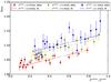 |
Fig. 11 Overestimate of the mock power spectrum determined from the likelihood method as a function of Pnoise/Praw, for different values of Pnoise. The curves illustrate the best fit model. |
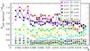 |
Fig. 12 Systematic uncertainty related to the correction of the noise-related bias in the likelihood method, relative to the statistical uncertainty, for each redshift bin. |
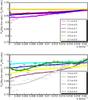 |
Fig. 13 Underestimate of the power spectrum due to the masking of the sky emission lines for the FT approach. The curves are polynomial fits to the measured k-dependent bias for each redshift bin. No strong sky lines enter the forest in 2.7 < z < 3.3, implying no systematic uncertainty in this redshift range. |
The masking of the sky emission lines is implemented in different ways in the two analysis methods. In the likelihood approach, where the relevant pixels are simply omitted, the masking procedure results in no measurable bias. For the FT approach, we estimate the impact of the masking procedure by applying it on mock spectra that do not include emission from sky lines. The result is illustrated in Fig. 13. No strong sky line enters the forest for the redshift range 2.7 < z < 3.3, which explains why no bias is observed in the corresponding redshift bins. The largest bias occurs for large-scale modes where most of the effect is related to the relative number of masked pixels in the forest. The effect on small scales is more sensitive to the distribution and size of the masked regions. The bias tends to decrease with increasing k, to become negligible near k = 0.02km s-1. It is modeled by a third-degree polynomial (except for the 4.3 < z < 4.5 redshift bin where a fourth-degree polynomial is used) that is used to correct the measured power spectrum. We assign a systematic uncertainty on the resulting power spectrum equal to the 30% of the correction. As illustrated in Fig. 14, the systematic uncertainty is greater at small k, but it remains subdominant compared to the statistical uncertainty for all modes.
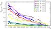 |
Fig. 14 Systematic uncertainty related to the masking of the sky lines in the FT approach, relative to the statistical uncertainty, for each redshift bin. |
Table 2 summarizes the sources of bias identified in both analysis methods. The final power spectra are corrected for these under- or overestimations. As explained above, we infer k- and z-dependent systematic uncertainties associated with these corrections. Their values are given along with the power spectrum measurements in Sect. 6.
Bias introduced at different steps of the analyses.
5.2. Instrumental uncertainties and associated systematics
The two main sources of instrumental uncertainties are related to the estimate of the noise and the resolution. The techniques to correct these two effects are respectively described in Sects. 2.3 and 2.4. Here we present the associated systematics.
The power spectrum of the noise is obtained by computing the Fourier transform of a “difference spectrum” between the individual exposures of a single quasar. In a similar way as in Fig. 1, we compare the side-band measurement of the noise (estimated as the flux rms in the 1330 < λRF < 1380 Å side-band of a quasar) either to the pipeline noise or to our determination of the noise from the difference power spectrum. Using the distribution of quasar redshifts, we show these distributions as a function of wavelength in the left-hand plot of Fig. 15: the red curve shows the ratio of the average pipeline noise over the side-band noise; the green curve is the ratio of our estimate of the pixel noise, using the correction factor given in Eq. (2), over the side-band noise. After correction, the distribution is flat in wavelength and centered on 1.0, as expected. The right-hand plot of Fig. 15 shows the distribution of the residuals after correction. Its spread provides an estimate of the remaining uncertainty on the noise. From a Gaussian fit as shown in right-hand plot of Fig. 15, we assign a conservative ~1.5% systematic error on the noise estimate.
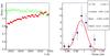 |
Fig. 15 Left: ratio of pipeline to side-band estimates of the noise as a function of the wavelength without correction (red dots) and when including the correction of Eq. (2) (green circles). Right: distribution of the residuals of the noise ratio including noise correction; the rms of the green distribution, ~1.5%, gives an estimate of the uncertainty on the noise correction. |
We applied a similar method to derive the systematic error related to the resolution. In this case, we plotted the ratio of our resolution measurement to the resolution given by the pipeline (red) as a function of the fiber number (see the left plot of Fig. 16). In green, the pipeline resolution is corrected by our model of Sect. 2.4. The rms of the residual distribution with respect to 1.0 yields a value of about 3% for the systematic error on the spectrograph resolution.
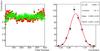 |
Fig. 16 Left: discrepancy between pipeline and arc lamp resolution as a function of the fiber number before correction (red dots) and after correction of Sect. 2.4 (green circles). This plot is obtained for the Cd line at ~4800 Å. Right: distribution of the residuals of the resolution correction; the rms of the green distribution, ~3.0%, provides an estimate of the uncertainty on the resolution correction. |
We determine the final impact of each of these two systematic effects using the data. We
increase, for instance, our estimate of the noise for all the quasar spectra selected for
the data analysis by the observed dispersion of 1.5%. We then apply the full procedure to
measure the 1D power spectrum P(k,z) with this new
estimate of the noise. Finally, for each bin, we compare the new power spectrum,
Pnew(k,z), to the nominal power spectrum
Pinit(k,z). We define the systematic error
to be  . This is a conservative approach
since we here consider a systematic effect acting in the same direction
for all the quasars. The impact on the power spectrum of these systematic uncertainties
are illustrated in Fig. 17. The systematic on the
noise estimate is the largest for low-redshift bins; with the cut we have applied on the
spectrum S/N, its contribution is at most of 70% of σstat. The
systematic on the resolution estimate becomes dominant, over all other sources of
uncertainties, on small scales for z < 3.0. The
stringent cut we have applied on the mean resolution in the forest
(
. This is a conservative approach
since we here consider a systematic effect acting in the same direction
for all the quasars. The impact on the power spectrum of these systematic uncertainties
are illustrated in Fig. 17. The systematic on the
noise estimate is the largest for low-redshift bins; with the cut we have applied on the
spectrum S/N, its contribution is at most of 70% of σstat. The
systematic on the resolution estimate becomes dominant, over all other sources of
uncertainties, on small scales for z < 3.0. The
stringent cut we have applied on the mean resolution in the forest
( km s-1), however, has limited this uncertainty by almost a factor 5 compared
to its value in the absence of such a cut.
km s-1), however, has limited this uncertainty by almost a factor 5 compared
to its value in the absence of such a cut.
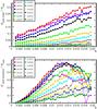 |
Fig. 17 Systematic uncertainty related to the estimate of the noise (upper plot) or of the spectrograph resolution (bottom plot), relative to the statistical uncertainty, for each redshift bin. |
6. Power spectrum measurement
We apply the methods presented previously to the BOSS data and measure the flux power spectrum in the Lyα forest region. It contains two components: the signal arising from H i absorption, and the background due to absorption by all species other than atomic hydrogen (hereafter “metals”). In this section, we explain how we separate each contribution and conclude by summarizing the obtained results.
Absorption at an observed wavelength λ receives contributions from any atomic species, i, absorbing at wavelength λi, if the absorption redshift zi + 1 = λ/λi satisfies zi < zqso. We want to subtract the background from metals. To do this, we use two methods that work for species with λi > λLyα and λi ~ λLyα.
For the first case, the wavelength of the metal line is far from Lyα. If its absorption falls in the Lyα forest of a quasar, then the Lyα absorption from the same redshift absorber is outside (bluer than) the forest wavelength range. It therefore presents no correlation with the Lyα absorption. The summed absorption at λ due to all such species can be determined by studying absorption at λ in quasars with zqso + 1 < λ/λLyα for which Lyα absorption makes no contribution. The subtraction of the background for this first case is described in Sect. 6.1. For the second case, atomic hydrogen and the metal species produce correlated absorption within the Lyα forest (Pieri et al. 2010). The 1D correlation function will have a peak at wavelength separations corresponding to hydrogen and metallic absorption at the same redshift: Δλ/λ = 1 − λi/λLyα. The main contribution in this second case comes from Si iii. The strategy adopted to subtract this second category of background is described in Sect. 6.2. Then, in Sect. 6.3, we present the final results in such a way that the reader can access directly the signal power spectrum and the different contaminating components.
6.1. Uncorrelated background subtraction
The uncorrelated background due to metal absorption in the Lyα forest cannot be estimated directly from the power spectrum measured in this region. We address this issue by estimating the background components in sidebands located at longer wavelengths than the Lyα forest region. We measure the power spectrum in these sidebands and subtract it from the Lyα power spectrum measured in the same gas redshift range. This method is purely statistical; we use different quasars to compute the Lyα forest and the metal power spectra for a given redshift bin. This approach is inspired by the method described in McDonald et al. (2006). However, our approach is simpler and more robust because it only relies on control samples and does not require any modeling.
In practice, we define two sidebands that correspond, in the quasar rest frame, to the wavelength ranges 1270 < λRF < 1380 Å and 1410 < λRF < 1520 Å. The power spectrum measured in the first sideband includes the contribution from all metals with λRF > 1380 Å, including absorption from Si iv and C iv. The second sideband also includes C iv but excludes the Si iv absorption. For our analysis, we use the first sideband (1270 < λRF < 1380 Å) to subtract the metal contribution in the power spectrum, and measurement in the second sideband constitutes an important consistency check.
We determine the metal power spectrum in the same observed wavelength range as the Lyα forest power spectrum from which it is being subtracted. For instance, for the first redshift bin, 2.1 < z < 2.3, we measure the power spectrum in the first sideband, corresponding to 3650 < λ < 4011 Å, i.e., using quasars with a redshift z ~ 1.9. Quasars in a given redshift window have their two sidebands corresponding to fixed observed wavelength windows, which in turn match a specific redshift window of Lyα forest.
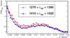 |
Fig. 18 Power spectrum PSB(k) computed for sideband regions above the Lyα forest region. The red dots and the blue squares are for the two sidebands defined in the rest frame by 1270 < λRF < 1380 Å and 1410 < λRF < 1520 Å respectively. Each power spectrum is fitted with a sixth-degree polynomial. |
The power spectra PSB(k) shown in Fig. 18 are obtained with ~40 000 quasars with redshift in the range 1.7 < z < 4.0, passing similar quality cuts as the quasars for the Lyα forest analysis. The shapes of PSB(k) are similar for the two sidebands. As expected, for the second sideband, corresponding to 1410 < λRF < 1520 Å, which excludes Si iv, the magnitude of PSB(k) is smaller. We fit the distribution PSB(k) with a sixth-degree polynomial. We use this fitted function as a template to parametrize the PSB(k) measured for each wavelength window (see Fig. 19).
As the shape and the magnitude of the power spectrum vary from one wavelength window to another, we have parameterized this as the product of the fixed shape obtained in Fig 18, with a variable first-degree polynomial, with two free parameters that are different for each wavelength window. This adequately fits the measured power in all the wavelength windows (see Fig. 19). From these parametric functions, we extract the value of the power spectrum PSB(k) for each k and for each Lyα redshift window.
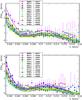 |
Fig. 19 Power spectrum P(k) computed for sideband regions above the Lyα forest region for different λ windows. Each λ region corresponds to one redshift bin. The top and bottom plots correspond respectively to the two sidebands defined in the rest frame by 1270 < λRF < 1380 Å and 1410 < λRF < 1520 Å. Each power spectrum is fitted by the product of the sixth-degree polynomial obtained in Fig. 18 and a first-degree polynomial in which the 2 parameters are free. |
The statistical uncertainty on PSB is strongest where we have the lowest number of quasars to measure the metal contribution. This occurs in the z ~ 2.2 redshift bin for which we only have ~400 quasars (at zqso ~ 1.7) instead of about 4000 on average for the other bins. For z ~ 2.2, the uncertainty on the metal correction, derived from the statistical precision on the first-degree polynomial fit, is around 10%.
An uncertainty on our metal correction will have the strongest impact relative to the measured P(k) in the Lyα region when the absolute P(k) has the lowest value. This again occurs for z ~ 2.2, which therefore constitutes the worst case both in terms of statistical uncertainty and relative level of the correction. Even in this worst case, the metal power spectrum is less than 10% of the Lyα power spectrum. The uncertainty of the metal correction is therefore less than 1% of the LyαP(k) across our whole sample.
6.2. Si iii cross-correlation
The correlated background due to absorption by Lyα and Si iii
from the same gas cloud along the quasar line of sight can be estimated directly in
the power spectrum. Since Si iii absorbs at λ = 1206.50 Å, it
appears in the data auto-correlation function
ξtot(v) = ⟨δ(x)δ(x + v) ⟩
as a bump at Δv = 2271 km s-1, and in the power spectrum as
wiggles with peak separations of
Δk = 2π/Δv = 0.0028km s-1.
Following the approach suggested by McDonald et al.
(2006), we model the Si iii structure as being equal to that of the
Lyα forest up to an overall normalization:
δtot = δ(v) + aδ(v + Δv)
where δ(v) is only for Lyα. The
corresponding correlation function is
 (12)and
the corresponding power spectrum
(12)and
the corresponding power spectrum  (13)where
ξ(v) and P(k) are
for Lyα-Lyα correlations. We clearly detect, in the
power spectrum, the oscillatory pattern due to the Si iii-Lyα
cross correlation (cf. Fig. 20), or equivalently a
peak near Δλ = 9.2 Å in the correlation function. We do not observe any
other significant metal features seen in Pieri et al.
(2010), such as Si ii lines (at 22.4 Å and 25.3 Å) or N v lines
(at 23.2 Å and 27.1Å). However, some weak contribution may be present from metals where
they do not produce signal distinct from each other or from the greater
Lyα signal.
(13)where
ξ(v) and P(k) are
for Lyα-Lyα correlations. We clearly detect, in the
power spectrum, the oscillatory pattern due to the Si iii-Lyα
cross correlation (cf. Fig. 20), or equivalently a
peak near Δλ = 9.2 Å in the correlation function. We do not observe any
other significant metal features seen in Pieri et al.
(2010), such as Si ii lines (at 22.4 Å and 25.3 Å) or N v lines
(at 23.2 Å and 27.1Å). However, some weak contribution may be present from metals where
they do not produce signal distinct from each other or from the greater
Lyα signal.
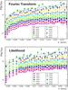 |
Fig. 20 One-dimensional Lyα forest power spectrum obtained with the Fourier transform method (top plot) and the likelihood method (bottom plot). The metal contribution estimated in Sect. 6.1 is subtracted. The power spectrum is fitted with the empirical function of Eq. (14). |
The measured normalization evolves with redshift roughly as
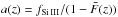 ,
where
is the mean transmitted fraction defined in Sect. 3.3. With a simple fit, we find a normalization factor
fSi III = 0.008 ± 0.001, similar to the value
f ~ 0.011 measured by McDonald et al.
(2006) on a sample of 3000 SDSS quasars, and in agreement with the value derived
in Sect. 7 from a completely independent fit to a
cosmological model.
,
where
is the mean transmitted fraction defined in Sect. 3.3. With a simple fit, we find a normalization factor
fSi III = 0.008 ± 0.001, similar to the value
f ~ 0.011 measured by McDonald et al.
(2006) on a sample of 3000 SDSS quasars, and in agreement with the value derived
in Sect. 7 from a completely independent fit to a
cosmological model.
6.3. Summary of experimental results
Figure 20 shows the one-dimensional Lyα forest power spectrum obtained with the Fourier transform and the likelihood method. Figure 21 demonstrates good agreement between the methods, although they are quite different in the treatment of the sky line masking, the noise subtraction, and the resolution correction. Moreover, the agreement with the previous SDSS measurements (McDonald et al. 2006) is also remarkable. The only significant discrepancy between SDSS and BOSS is observed for the low z and high k region where the noise subtraction is difficult. The uncertainty in this region is covered either by the use of the systematics errors given in Sect. 5.2 or by introducing nuisance parameters. The latter option is the one we have chosen for the cosmological interpretation of our results (see Sect. 7.2).
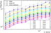 |
Fig. 21 Comparison of the 1D Lyα forest power spectrum obtained in BOSS and in SDSS (see McDonald et al. 2006) over the redshift range, z = [2.1−4.3]. For BOSS, we show the results for the two methods, Fourier transform and likelihood, and we use the same k bins as in McDonald et al. (2006). |
P1D results obtained with the FT method for each k and z bin (top table), and correlation matrices between k bins for each z bin (following tables).
To compare the measured power spectrum for SDSS and BOSS, and also to compare the results
of the Fourier transform and the likelihood methods in a quantitively way, we define an
empirical function Pemp with which we fit each power spectrum
distribution. This function, written in Eq. (14), has five free physical parameters: an amplitude
AF corresponding to the amplitude of the
power spectrum at the pivot mode k0 and redshift
z0, a slope
nF = dlnP/dlnk|(k0,z0),
a curvature
αF = dlnnF/dlnk|(k0,z0),
and two parameters, BF and
βF, that model the redshift evolution of
the power spectrum. In addition, we introduce nuisance parameters to take the correlation
between H i and Si iii into account (parameter a in Eq.
(14)), and the imperfection of our
resolution and noise models. We choose a pivot point in the middle of our measurements,
k0 = 0.009 km s-1 and
z0 = 3.0. The results of the fits are summarized in Table
3. Agreement between the different methods and
datasets is good. All five parameters are within 1 or 2σ of one another.
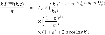 (14)Tables
4 and 5
summarize, for each redshift bin, the results for the 1D Lyα forest power
spectrum. They are available in their entirety at the CDS. The different components
(P1D, Pnoise and
Pmetals) are given in these tables. In
Pmetals we consider only the uncorrelated background
computed in Sect. 6.1. The last two columns
represent the statistical and systematical uncertainty on
P1D. We added in quadrature all the
systematic uncertainties studied in Sect. 5.2. The
correlation matrices are illustrated in Fig. 22 for
the first eight redshift bins that are used in Sect. 7 for the cosmological interpretation. The maximum correlation is at the level
of ~20% for neighboring k-modes, and the correlation rapidly drops to
<10%.
(14)Tables
4 and 5
summarize, for each redshift bin, the results for the 1D Lyα forest power
spectrum. They are available in their entirety at the CDS. The different components
(P1D, Pnoise and
Pmetals) are given in these tables. In
Pmetals we consider only the uncorrelated background
computed in Sect. 6.1. The last two columns
represent the statistical and systematical uncertainty on
P1D. We added in quadrature all the
systematic uncertainties studied in Sect. 5.2. The
correlation matrices are illustrated in Fig. 22 for
the first eight redshift bins that are used in Sect. 7 for the cosmological interpretation. The maximum correlation is at the level
of ~20% for neighboring k-modes, and the correlation rapidly drops to
<10%.
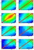 |
Fig. 22 Correlation matrices between the different k-modes for the first 8 redshift bins (z = [2.1−3.7]), smoothed by 2D second-degree polynomials, for the FT method. The color range is identical in all 8 plots, with red for all values above 0.25. |
7. Cosmological constraints
In this paper, we present a preliminary cosmological interpretation of our results. Our intention is to demonstrate the improvements in our measurements over the previous publication of SDSS presented in McDonald et al. (2006). We use an approach developed by Viel & Haehnelt (2006). This method is well adapted to the statistical accuracy of SDSS and is sufficient to give some results on the two cosmological parameters (σ8,ns) from our measurement of the 1D power spectrum.
In this interpretation, we only use the first eight redshift bins (i.e. z = [2.1−3.7]) as recommended in Viel & Haehnelt (2006). Moreover, to break the degeneracies between the cosmological parameters, we use a constraint on H0 that encompasses the measurements of Riess et al. (2011) and of Planck Collaboration (2013). This section should be seen as an exploration of potential cosmology from the 1D power spectrum.
As was shown in the previous section, the FT and the likelihood methods yield compatible results. We therefore restrict the cosmological fits of this section to the power spectrum obtained with the Fourier transform only.
7.1. Simulations
We computed the constraints from our measurements of the flux power spectrum following Viel & Haehnelt (2006) and Viel et al. (2009) where all the details can be found. We only give a brief summary here.
They used a grid of full hydrodynamical simulations run with the Tree-smoothed particle hydrodynamics code gadget-2 (Springel 2005) to model the nonlinear relation between the flux and the matter power spectra. The flux power spectrum was calculated using a second-order Taylor expansion (without cross terms). They ran several hydrodynamical simulations around the best estimated value for each cosmological and astrophysical parameter to compute the derivatives required for the Taylor expansion. The central cosmology used in the simulation grid is a ΛCDM model with σ8 = 0.85, ns = 0.95, Ωm = 0.26, and H0 = 72 km s-1 Mpc-1. The cosmological parameters are close to the values obtained by WMAP (Hinshaw et al. 2013), and the predicted flux statistics are derived by expanding around a model with γ ~ 1. This parameter defines the density-temperature relation of the IGM by the approximate relation T = T0(1 + δ)γ−1.
More complex astrophysical effects on statistics of the Lyα flux have been discussed in Viel et al. (2013), where it has been explicitly shown that the overall distribution of the gas in the T − ρ plane can affect the flux power in a redshift- and scale-dependent way for different physical models that include active galactic nuclei feedback or galactic winds. The effect is of similar magnitude as the statistical uncertainty of the data. A robust and conservative analysis of the 1D power should properly take the impact that astrophysics has on the final observable into account, and model this to a high level of precision. These effects have not been addressed in this work since the simulations used do not allow such refinements. It is however unlikely that the scale and redshift dependence of feedback models on the flux power is similar to that induced by cosmological parameters.
The standard simulations corresponded to a box of length L = 60 h-1 Mpc with 2 × 4003 (gas + dark matter) particles. They are corrected for box size effects using simulations with the same number of particles but L = 120 h-1 Mpc, and for resolution effects using simulations with L = 60 h-1 Mpc and 2 × 5123 particles.
7.2. Parameters
We have introduced four categories of parameters that are floated in the maximization of the likelihood. The first category describes the cosmological model in the simplest case of ΛCDM assuming a flat Universe with a zero neutrino mass. The second category models the astrophysics within the IGM and the relation between temperature and density for the gas. The purpose of the third category is to describe the imperfections of our measurement of the 1D power spectrum. By fitting the parameters of the latter category, we improve significantly the goodness of the fit but we reduce the sensitivity on the other parameters. Finally, a last parameter allows for a residual contamination from damped Lyα systems in our selected sample of quasar lines of sight.
-
Cosmological parameters: our ΛCDM cosmology is described by the fluctuation amplitude of the matter power spectrum σ8, the spectral index of primordial density fluctuations, ns, the matter density Ωm, and the Hubble constant H0.
-
Astrophysical parameters: two parameters describe the effective optical depth assuming a power law evolution,
![Mathematical equation: \hbox{$\tau_{\rm eff}(z) = \tau_{{\rm eff,}z\,=\,3}^A\times [(1+z)/4 ]^{\tau_{\rm eff}^S}$}](/articles/aa/full_html/2013/11/aa22130-13/aa22130-13-eq344.png) .
The evolution with redshift of γ and T0
are also modeled with power laws. For the temperature, we have two parameters:
.
The evolution with redshift of γ and T0
are also modeled with power laws. For the temperature, we have two parameters:
 , the
temperature at z = 3, and the slope (or exponent)
, the
temperature at z = 3, and the slope (or exponent)
 .
Similarly for γ, we have two parameters:
.
Similarly for γ, we have two parameters:
 , the
value at z = 3, and the slope
γS. To account for the effect of
the correlated Si iii absorption, we introduce a multiplicative term,
1 + a2 + 2acos(vk)
with
, the
value at z = 3, and the slope
γS. To account for the effect of
the correlated Si iii absorption, we introduce a multiplicative term,
1 + a2 + 2acos(vk)
with  as in Sect. 6.2 following the suggestion of
McDonald et al. (2006). The parameter
fSi III is free in the fit, and v
is fixed at 2271 km s-1.
as in Sect. 6.2 following the suggestion of
McDonald et al. (2006). The parameter
fSi III is free in the fit, and v
is fixed at 2271 km s-1. -
Nuisance parameters: we take the imperfection of our resolution model into account by floating one multiplicative term. We allow for imperfection in our noise estimate by floating eight additive terms (one for each redshift bin).
-
Damped Lyα system: in McDonald et al. (2005a), the effect of the DLA was modeled on the power spectrum. We included this correction using their k dependence. We have the possibility of fitting the amplitude of this correction with the parameter Adamp.
7.3. Fit to the SDSS and BOSS data
For a given cosmological model defined by the n cosmological,
astrophysical and nuisance parameters
Θ = (θ1,...,θn),
and for a data set of power spectra
P(ki,zj)
measured with Gaussian experimental errors
σi,j, the likelihood function can be
written as ![Mathematical equation: \begin{eqnarray*} {\cal L}\bigl(P,\sigma;\Theta\bigr) = \prod_{i,j}\frac{1}{\sqrt{2\pi}\sigma_{i,j}} \exp\left( -\frac{[P(k_i,z_j) - P^{\rm th}(k_i,z_j) ]^2}{2\sigma_{i,j}^2} \right)\nonumber \end{eqnarray*}](/articles/aa/full_html/2013/11/aa22130-13/aa22130-13-eq359.png) where
Pth(ki,zj)
is the predicted value of the power spectrum for the bin
ki and redshift
zj.
where
Pth(ki,zj)
is the predicted value of the power spectrum for the bin
ki and redshift
zj.
In the rest of this paper, we adopt a χ2 notation, which
means that the following quantity is minimized:  (15)The
second term of Eq. (15) represents the
external constraint on H0. Because the value obtained from HST
observations (
(15)The
second term of Eq. (15) represents the
external constraint on H0. Because the value obtained from HST
observations ( )
given in Riess et al. (2011) and the value from
Planck (
)
given in Riess et al. (2011) and the value from
Planck (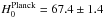 )
given in Planck Collaboration (2013) differ by over
2σ, we write this H0 constraint so as to
give equal weight to both measurements:
)
given in Planck Collaboration (2013) differ by over
2σ, we write this H0 constraint so as to
give equal weight to both measurements: 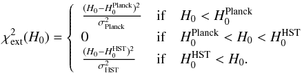 The
purpose of this section is to compare the SDSS and BOSS measured power spectra. We
therefore use the same binning in k and z and the same
strategy for the fit as in McDonald et al. (2006).
In this study, the minimization of χ2(P,σ;Θ)
was performed with the MINUIT package (James &
Ross 1975). Figure 23 shows the
P(ki,zj)
measurements of the power spectrum with the
Pth(k,z) function adjusted by the
minimization of χ2(P,σ;Θ). The results of the
fit are given in Table 6, and the determination of
the error with a frequentist interpretation is discussed in the next paragraph.
The
purpose of this section is to compare the SDSS and BOSS measured power spectra. We
therefore use the same binning in k and z and the same
strategy for the fit as in McDonald et al. (2006).
In this study, the minimization of χ2(P,σ;Θ)
was performed with the MINUIT package (James &
Ross 1975). Figure 23 shows the
P(ki,zj)
measurements of the power spectrum with the
Pth(k,z) function adjusted by the
minimization of χ2(P,σ;Θ). The results of the
fit are given in Table 6, and the determination of
the error with a frequentist interpretation is discussed in the next paragraph.
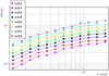 |
Fig. 23 Fit of the power spectrum measured with BOSS in the range z = [2.1−3.7]; the z and k binning of McDonald et al. (2006) is adopted. |
Results of the fit (frequentist approach) to the measured P(ki,zj) for the first eight redshift bins covering the z = [2.1−3.7] region.
7.4. Frequentist interpretation
Most recent Lyα analyses use Markov Chain Monte Carlo simulations (Viel et al. 2010) with Bayesian inference. The debate between the Bayesian and the frequentist statistical approaches is beyond the scope of this paper. The philosophical difference between the two methods should not generally lead, in the end, to major differences in determining physical parameters and their confidence intervals when the parameters stay in a physical region (see Yèche et al. 2006).
Our work is based on the “frequentist” (or “classical”) confidence-level method originally defined by Neyman (1937). This avoids any potential bias due to the choice of priors. In addition, we have also found ways to improve the calculation speed, which gives our program some advantages over Bayesian programs.
We first determine the minimum  of
χ2(x,σx;Θ)
leaving all the cosmological parameters free. Then, to set a confidence level (CL) on any
individual cosmological parameter θi, we scan
the variable θi: for each fixed value of
θi, we again minimize
χ2(x,σx;Θ)
but with n − 1 free parameters. The χ2
difference,
Δχ2(θi),
between the new minimum and , allows us to
compute the CL on the variable, assuming that the experimental errors are Gaussian,
of
χ2(x,σx;Θ)
leaving all the cosmological parameters free. Then, to set a confidence level (CL) on any
individual cosmological parameter θi, we scan
the variable θi: for each fixed value of
θi, we again minimize
χ2(x,σx;Θ)
but with n − 1 free parameters. The χ2
difference,
Δχ2(θi),
between the new minimum and , allows us to
compute the CL on the variable, assuming that the experimental errors are Gaussian,
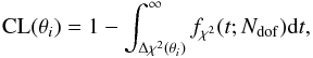 (16)with
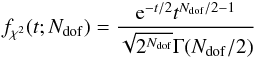 (17)where
Γ is the Gamma function and the number of degrees of freedom
Ndof is equal to 1. This method can be easily extended to
two variables. In this case, the minimizations are performed for n − 2
free parameters and the confidence level
CL(θi,θj)
is derived from Eq. (16) with
Ndof = 2.
(17)where
Γ is the Gamma function and the number of degrees of freedom
Ndof is equal to 1. This method can be easily extended to
two variables. In this case, the minimizations are performed for n − 2
free parameters and the confidence level
CL(θi,θj)
is derived from Eq. (16) with
Ndof = 2.
By definition, this frequentist approach does not require any marginalization to determine the sensitivity on a single individual cosmological parameter. Moreover, in contrast to Bayesian treatment, no prior on the cosmological parameters is needed. With this approach, the correlations between the variables are naturally taken into account and the minimization fit can explore the whole phase space of the cosmological, astrophysics, and nuisance parameters.
It is difficult to define the goodness of fit to the data with the absolute value of
 since we do not know the actual number of degrees of freedom of our problem because of
correlations between the fit parameters. Therefore, we perform 1000 simulations of the
measured power spectrum (96 measurements) and repeat the fit for each simulation. The
distribution of the χ2 can be used to derive the goodness of
fit. A fit of the distribution of Fig. 24 indicates
a number of degrees of freedom equal to 87.6 ± 0.4. The fraction of simulations having a
χ2 value higher than is six
percent.
since we do not know the actual number of degrees of freedom of our problem because of
correlations between the fit parameters. Therefore, we perform 1000 simulations of the
measured power spectrum (96 measurements) and repeat the fit for each simulation. The
distribution of the χ2 can be used to derive the goodness of
fit. A fit of the distribution of Fig. 24 indicates
a number of degrees of freedom equal to 87.6 ± 0.4. The fraction of simulations having a
χ2 value higher than is six
percent.
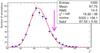 |
Fig. 24 Distribution of the χ2 obtained for 1000 simulations reproducing the 1D power spectrum measured by BOSS. The mean of the distribution is 87.8 and a fit of the distribution following a χ2 law defined in Eq. (17) gives a number of degrees of freedom equal to 87.6 ± 0.4. |
7.5. Results on σ8 and ns
Table 6 shows the results for the cosmological and the astrophysical parameters. Since the hydrodynamical simulations are preliminary versions of simulations that we are currently developing, we only focus here on the measurement of the two cosmological parameters σ8 and ns in the case of ΛCDM, assuming a flat Universe with three neutrinos with ∑ mν = 0. In this interpretation section, the other parameters should be considered as nuisance parameters, and the constraints obtained are only indicative. They will be refined in future work. Figures 25 and 26 present the confidence level obtained with Eq. (16) on ns and σ8. The central values of the fits on the SDSS measurements of McDonald et al. (2006) and on the BOSS measurements agree within 1σ. The comparison of the confidence level curves shows an improvement by a factor 2–3 in the constraint on these parameters with the BOSS data compared to the SDSS data. We measure σ8 = 0.83 ± 0.03 and ns = 0.97 ± 0.02 in the H i absorption range z = [2.1−3.7].
Since the two measurements of H0 by HST and by Planck are not fully consistent, we have chosen to use a conservative constraint on H0 that encompasses both and has a constant probability between the two measurements.
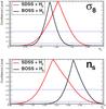 |
Fig. 25 Confidence level for the σ8 and ns cosmological parameters with a frequentist interpretation. The red and black curves are obtained respectively for SDSS and BOSS measurements of the power spectrum. |
In our quasar selection, we removed a large portion of the DLA. Therefore in our likelihood we have fixed to zero the amplitude Adamp of the component modeling the effect of the DLA in the power spectrum. If we float this parameter, we get Adamp = 0.14 ± 0.10, which is close to 0 as expected, and the values of σ8 and ns are unchanged.
The possible systematic uncertainties are included through nuisance parameters in the fit. The errors on σ8 and ns are not dominated by a unique category of parameters. Smaller errors by factor ~2 (respectively ~3) would be obtained on both parameters if we ignore nuisance parameters (resp. astrophysical parameters).
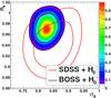 |
Fig. 26 2D confidence level contours for the σ8 and ns cosmological parameters with a frequentist interpretation. The red and black curves are obtained respectively for SDSS and BOSS measurements of the power spectrum. |
7.6. Discussion and prospects for future simulations
The preliminary cosmological results presented in the previous section are based on a set of hydrodynamical simulations by Viel & Haehnelt (2006), which are sufficient for our purposes but can be improved to meet the more stringent requirements of the BOSS survey. The restriction to only eight redshift bins is dictated by the set of simulations currently available for the analysis. Our next goal is to use the full redshift information in the 1D power spectrum, with all twelve redshift bins up to z = 4.5. To this end, we are following two lines of research, which will be presented in forthcoming publications. One is to upgrade the quality of the hydrodynamical simulations for the Lyman-α forest, both in resolution (i.e. number of particles) and box size. The other is to include massive neutrinos in our hydrodynamical simulations at the sensitivity of the BOSS survey, along with a number of technical and conceptual improvements, with the aim of constraining or measuring the sum of neutrino masses.
8. Conclusions
We have developed two independent methods for measuring the 1D power spectrum of the transmitted flux in the Lyα forest. The first method is based on a Fourier transform, and the second approach relies upon a maximum likelihood estimator. The two methods are independent and present different systematic uncertainties owing to the techniques used to mask pixels contaminated by sky emission lines or to take the spectrograph resolution and the noise contribution to the Lyα power spectrum into account, which differ in the two approaches. Determining the noise level in the data spectra was subject to a novel treatment, because of its significant impact on the derived power spectrum.
We applied these two methods to 13 821 quasar spectra from SDSS-III/BOSS, that were selected from a larger sample of almost 90 000 DR9 BOSS spectra on the basis of their high quality, high S/N, and the low value of the spectral resolution. The power spectra measured using either method are in good agreement over all twelve redshift bins from ⟨z⟩ = 2.2 to ⟨z⟩ = 4.4. We determined the systematic uncertainties on our measurements coming both from the analysis method and from our knowledge of the instrument characteristics.
We presented a preliminary cosmological interpretation of our experimental results, along the lines of Viel & Haehnelt (2006), limiting the analysis to the first eight redshift bins up to z = 3.7. The improvement in precision over previous studies from SDSS (McDonald et al. 2006) allows for a factor 2–3 tighter constraints on relevant cosmological parameters. In particular, for a ΛCDM model and using a constraint on H0 encompassing measurements from the HST and from Planck, we measure σ8 = 0.83 ± 0.03 and ns = 0.97 ± 0.02 in the H i absorption range 2.1 < z < 3.7.
These results were obtained by assuming a flat ΛCDM model with no massive neutrinos. In the near future, we will update the cosmological interpretation of our results by using the full information contained in the 1D power spectrum over all twelve redshift bins up to z = 4.5. This will be done thanks a new set of hydrodynamical simulations for the Lyα forest that we will run with an upgrade in both resolution and box size to match the sensitivity of our measurement and, in addition, which will include massive neutrinos.
http://www.fftw.org The FFTW package was developed by M. Frigo and S. G. Johnson, 1998.
Acknowledgments
Funding for SDSS-III has been provided by the Alfred P. Sloan Foundation, the Participating Institutions, the National Science Foundation, and the U.S. Department of Energy. The SDSS-III web site is http://www.sdss3.org/. The BOSS French Participation Group is supported by Agence Nationale de la Recherche under grant ANR-08-BLAN-0222. A.B., N.P.-D., G.R., and Ch.Y. acknowledge support from grant ANR-11-JS04-011-01 of Agence Nationale de la Recherche. M.V. is supported by ERC-StG “CosmoIGM”. SDSS-III is managed by the Astrophysical Research Consortium for the Participating Institutions of the SDSS-III Collaboration including the University of Arizona, the Brazilian Participation Group, Brookhaven National Laboratory, University of Cambridge, University of Florida, the French Participation Group, the German Participation Group, the Instituto de Astrofisica de Canarias, the Michigan State/Notre Dame/JINA Participation Group, Johns Hopkins University, Lawrence Berkeley National Laboratory, Max Planck Institute for Astrophysics, New Mexico State University, New York University, the Ohio State University, the Penn State University, University of Portsmouth, Princeton University, University of Tokyo, the University of Utah, Vanderbilt University, University of Virginia, University of Washington, and Yale University.
References
- Abazajian, K. N., Adelman-McCarthy, J. K., Agüeros, M. A., et al. 2009, ApJS, 182, 543 [NASA ADS] [CrossRef] [Google Scholar]
- Abel, T., & Haehnelt, M. G. 1999, ApJ, 520, L13 [NASA ADS] [CrossRef] [Google Scholar]
- Ahn, C. P., Alexandroff, R., Allen de Prieto, C., et al. 2012, ApJS, 203, 21 [NASA ADS] [CrossRef] [Google Scholar]
- Aihara, H., Allen de Prieto, C., An, D., et al. 2011, ApJS, 193, 29 [NASA ADS] [CrossRef] [Google Scholar]
- Alcock, C., & Paczynski, B. 1979, Nature, 281, 358 [NASA ADS] [CrossRef] [Google Scholar]
- Bi, H. G., Boerner, G., & Chu, Y. 1992, A&A, 266, 1 [NASA ADS] [Google Scholar]
- Bolton, A. S., Schlegel, D. J., Aubourg, É., et al. 2012, AJ, 144, 144 [NASA ADS] [CrossRef] [Google Scholar]
- Bond, J. R., Jaffe, A. H., & Knox, L. 1998, Phys. Rev. D, 57, 2117 [NASA ADS] [CrossRef] [Google Scholar]
- Bovy, J., Hennawi, J. F., Hogg, D. W., et al. 2011, ApJ, 729, 141 [NASA ADS] [CrossRef] [Google Scholar]
- Busca, N. G., Delubac, T., Rich, J., et al. 2013, A&A, 552, A96 [NASA ADS] [CrossRef] [EDP Sciences] [Google Scholar]
- Cen, R., Miralda-Escudé, J., Ostriker, J. P., & Rauch, M. 1994, ApJ, 437, L9 [Google Scholar]
- Croft, R. A. C., Weinberg, D. H., Katz, N., & Hernquist, L. 1998, ApJ, 495, 44 [NASA ADS] [CrossRef] [Google Scholar]
- Croft, R. A. C., Weinberg, D. H., Pettini, M., Hernquist, L., & Katz, N. 1999, ApJ, 520, 1 [NASA ADS] [CrossRef] [Google Scholar]
- Croft, R. A. C., Weinberg, D. H., Bolte, M., et al. 2002, ApJ, 581, 20 [NASA ADS] [CrossRef] [Google Scholar]
- Dawson, K. S., Schlegel, D. J., Ahn, C. P., et al. 2013, AJ, 145, 10 [Google Scholar]
- Desjacques, V., Nusser, A., & Sheth, R. K. 2007, MNRAS, 374, 206 [NASA ADS] [CrossRef] [Google Scholar]
- Doi, M., Tanaka, M., Fukugita, M., et al. 2010, AJ, 139, 1628 [NASA ADS] [CrossRef] [Google Scholar]
- Eisenstein, D. J., Weinberg, D. H., Agol, E., et al. 2011, AJ, 142, 72 [Google Scholar]
- Feng, L.-L., & Fang, L.-Z. 2000, ApJ, 535, 519 [NASA ADS] [CrossRef] [Google Scholar]
- Font-Ribera, A., McDonald, P., & Miralda-Escudé, J. 2012, JCAP, 1, 1 [Google Scholar]
- Fukugita, M., Ichikawa, T., Gunn, J. E., et al. 1996, AJ, 111, 1748 [NASA ADS] [CrossRef] [Google Scholar]
- Gaztañaga, E., & Croft, R. A. C. 1999, MNRAS, 309, 885 [NASA ADS] [CrossRef] [Google Scholar]
- Gnedin, N. Y. 1998, MNRAS, 299, 392 [Google Scholar]
- Gunn, J. E., Carr, M., Rockosi, C., et al. 1998, AJ, 116, 3040 [NASA ADS] [CrossRef] [Google Scholar]
- Gunn, J. E., Siegmund, W. A., Mannery, E. J., et al. 2006, AJ, 131, 2332 [NASA ADS] [CrossRef] [Google Scholar]
- Hernquist, L., Katz, N., Weinberg, D. H., & Miralda-Escudé, J. 1996, ApJ, 457, L51 [NASA ADS] [CrossRef] [Google Scholar]
- Hinshaw, G., Larson, D., Komatsu, E., et al. 2013, ApJS, 208, 19 [NASA ADS] [CrossRef] [Google Scholar]
- Hui, L., & Gnedin, N. Y. 1997, MNRAS, 292, 27 [Google Scholar]
- Hui, L., Gnedin, N. Y., & Zhang, Y. 1997, ApJ, 486, 599 [NASA ADS] [CrossRef] [MathSciNet] [Google Scholar]
- Hui, L., Stebbins, A., & Burles, S. 1999, ApJ, 511, L5 [NASA ADS] [CrossRef] [Google Scholar]
- Hui, L., Burles, S., Seljak, U., et al. 2001, ApJ, 552, 15 [NASA ADS] [CrossRef] [Google Scholar]
- James, F., & Ross, M. 1975, Comput. Phys. Commun., 10, 343 [NASA ADS] [CrossRef] [PubMed] [Google Scholar]
- Kaiser, N. 1987, MNRAS, 227, 1 [NASA ADS] [CrossRef] [Google Scholar]
- Kim, T.-S., Viel, M., Haehnelt, M. G., Carswell, B., & Cristiani, S. 2004a, MNRAS, 351, 1471 [NASA ADS] [CrossRef] [Google Scholar]
- Kim, T.-S., Viel, M., Haehnelt, M. G., Carswell, R. F., & Cristiani, S. 2004b, MNRAS, 347, 355 [NASA ADS] [CrossRef] [Google Scholar]
- Kirkby, D., Margala, D., Slosar, A., et al. 2013, JCAP, 3, 24 [Google Scholar]
- Kirkpatrick, J. A., Schlegel, D. J., Ross, N. P., et al. 2011, ApJ, 743, 125 [NASA ADS] [CrossRef] [Google Scholar]
- LeGoff, J. M., Magneville, C., Rollinde, E., et al. 2011, A&A, 534, A135 [NASA ADS] [CrossRef] [EDP Sciences] [Google Scholar]
- Lee, K.-G., Bailey, S., Bartsch, L. E., et al. 2013, AJ, 145, 69 [Google Scholar]
- Lynds, R. 1971, ApJ, 164, L73 [NASA ADS] [CrossRef] [Google Scholar]
- McDonald, P. 2003, ApJ, 585, 34 [NASA ADS] [CrossRef] [Google Scholar]
- McDonald, P., & Eisenstein, D. J. 2007, Phys. Rev. D, 76, 063009 [NASA ADS] [CrossRef] [Google Scholar]
- McDonald, P., & Miralda-Escudé, J. 1999, ApJ, 518, 24 [NASA ADS] [CrossRef] [Google Scholar]
- McDonald, P., Miralda-Escudé, J., Rauch, M., et al. 2000, ApJ, 543, 1 [NASA ADS] [CrossRef] [Google Scholar]
- McDonald, P., Seljak, U., Cen, R., Bode, P., & Ostriker, J. P. 2005a, MNRAS, 360, 1471 [NASA ADS] [CrossRef] [Google Scholar]
- McDonald, P., Seljak, U., Cen, R., et al. 2005b, ApJ, 635, 761 [NASA ADS] [CrossRef] [Google Scholar]
- McDonald, P., Seljak, U., Burles, S., et al. 2006, ApJS, 163, 80 [NASA ADS] [CrossRef] [Google Scholar]
- Meiksin, A. A. 2009, Rev. Mod. Phys., 81, 1405 [NASA ADS] [CrossRef] [Google Scholar]
- Miralda-Escudé, J., & Rees, M. J. 1993, MNRAS, 260, 617 [NASA ADS] [Google Scholar]
- Neyman, J. 1937, Phil. Trans. Royal Soc. London, Series A, 236, 333 [Google Scholar]
- Nusser, A., & Haehnelt, M. 1999, MNRAS, 303, 179 [NASA ADS] [CrossRef] [Google Scholar]
- Palanque-Delabrouille, N., Yeche, C., Myers, A. D., et al. 2011, A&A, 530, A122 [NASA ADS] [CrossRef] [EDP Sciences] [Google Scholar]
- Pâris, I., Petitjean, P., Rollinde, E., et al. 2011, A&A, 530, A50 [NASA ADS] [CrossRef] [EDP Sciences] [Google Scholar]
- Pâris, I., Petitjean, P., Aubourg, É., et al. 2012, A&A, 548, A66 [NASA ADS] [CrossRef] [EDP Sciences] [Google Scholar]
- Pieri, M. M., Frank, S., Weinberg, D. H., Mathur, S., & York, D. G. 2010, ApJ, 724, L69 [NASA ADS] [CrossRef] [Google Scholar]
- Planck Collaboration 2013, A&A, submitted [arXiv:1303.5076] [Google Scholar]
- Riess, A. G., Macri, L., Casertano, S., et al. 2011, ApJ, 730, 119 [NASA ADS] [CrossRef] [Google Scholar]
- Ross, N. P., Myers, A. D., Sheldon, E. S., et al. 2012, ApJS, 199, 3 [NASA ADS] [CrossRef] [Google Scholar]
- Schlegel, D. J., Finkbeiner, D. P., & Davis, M. 1998, ApJ, 500, 525 [NASA ADS] [CrossRef] [Google Scholar]
- Seljak, U. 1998, ApJ, 506, 64 [Google Scholar]
- Seljak, U., Makarov, A., McDonald, P., et al. 2005, Phys. Rev. D, 71, 103515 [NASA ADS] [CrossRef] [Google Scholar]
- Slosar, A., Font-Ribera, A., Pieri, M. M., et al. 2011, JCAP, 9, 1 [Google Scholar]
- Slosar, A., Iršič, V., Kirkby, D., et al. 2013, JCAP, 4, 26 [Google Scholar]
- Smee, S. A., Gunn, J. E., Uomoto, A., et al. 2013, AJ, 146, 32 [Google Scholar]
- Smith, J. A., Tucker, D. L., Kent, S., et al. 2002, AJ, 123, 2121 [Google Scholar]
- Springel, V. 2005, MNRAS, 364, 1105 [NASA ADS] [CrossRef] [Google Scholar]
- Stoughton, C., Lupton, R. H., Bernardi, M., et al. 2002, AJ, 123, 485 [NASA ADS] [CrossRef] [Google Scholar]
- Viel, M., & Haehnelt, M. G. 2006, MNRAS, 365, 231 [NASA ADS] [CrossRef] [Google Scholar]
- Viel, M., Haehnelt, M. G., & Springel, V. 2004, MNRAS, 354, 684 [NASA ADS] [CrossRef] [Google Scholar]
- Viel, M., Bolton, J. S., & Haehnelt, M. G. 2009, MNRAS, 399, L39 [NASA ADS] [CrossRef] [Google Scholar]
- Viel, M., Haehnelt, M. G., & Springel, V. 2010, JCAP, 6, 15 [Google Scholar]
- Viel, M., Schaye, J., & Booth, C. M. 2013, MNRAS, 429, 1734 [NASA ADS] [CrossRef] [Google Scholar]
- Yèche, C., Ealet, A., Réfrégier, A., et al. 2006, A&A, 448, 831 [NASA ADS] [CrossRef] [EDP Sciences] [Google Scholar]
- Yèche, C., Petitjean, P., Rich, J., et al. 2010, A&A, 523, A14 [NASA ADS] [CrossRef] [EDP Sciences] [Google Scholar]
- York, D. G., Adelman, J., Anderson, Jr., J. E., et al. 2000, AJ, 120, 1579 [Google Scholar]
- Zhang, Y., Anninos, P., & Norman, M. L. 1995, ApJ, 453, L57 [NASA ADS] [CrossRef] [Google Scholar]
All Tables
Summary of main quasar selection cuts and fraction of quasars passing previous cuts rejected at each step.
P1D results obtained with the FT method for each k and z bin (top table), and correlation matrices between k bins for each z bin (following tables).
Results of the fit (frequentist approach) to the measured P(ki,zj) for the first eight redshift bins covering the z = [2.1−3.7] region.
All Figures
|
Fig. 1 Ratio of the pipeline noise estimate to the actual flux dispersion in the spectra. The blue squares denote this ratio as estimated from the quasar 1330 < λRF < 1380 Å and 1450 < λRF < 1500 Å sidebands. The red points indicate the correction from our procedure (Eq. (2)) as a function of mean forest wavelength. |
| In the text | |
|
Fig. 2 Average power spectra of the raw (filled dots) and of the difference (open circles) signal for three ranges in Lyα redshifts. |
| In the text | |
|
Fig. 3 Comparison of the resolution given by the pipeline (blue circles) and our computation (purple crosses) for arc lamp or sky line as a function of fiber number (i.e. position of spectrum on CCD). Upper left: comparison with arc lamp for a mercury line at ~3650 Å. Upper right: comparison with arc lamp for a cadmium line at ~4800 Å. Lower left: comparison with arc lamp for a mercury line at ~5461 Å. Lower right: comparison with the OI sky line at ~5577 Å. |
| In the text | |
|
Fig. 4 Top: correction of the pipeline resolution for spectra in the middle of the CCD (fiber numbers ~250). The curve is the best second-order polynomial fit to the measurements at the arc-lamp wavelengths. Bottom: 2D correction table of the pipeline resolution as a function of fiber number (ie. position of spectrum on CCD) and wavelength. |
| In the text | |
|
Fig. 5 Redshift distribution of the 13 821 quasars selected in the analysis, and mean redshift distribution of each z-sector of their Lyα forest. |
| In the text | |
|
Fig. 6 Average quasar spectra in five redshift bins. All spectra are normalized at λ = 1280 Å. |
| In the text | |
|
Fig. 7 Product of the quasar continuum
Cq(λ,zqso)
by the mean transmitted flux fraction |
| In the text | |
|
Fig. 8 Top: mean transmitted fraction
|
| In the text | |
|
Fig. 9 Mean of δ(λ) as a function of wavelength in Å. Systematic offsets from zero are seen at the 2% level due to imperfections in the spectrograph calibration. |
| In the text | |
|
Fig. 10 Window function |
| In the text | |
|
Fig. 11 Overestimate of the mock power spectrum determined from the likelihood method as a function of Pnoise/Praw, for different values of Pnoise. The curves illustrate the best fit model. |
| In the text | |
|
Fig. 12 Systematic uncertainty related to the correction of the noise-related bias in the likelihood method, relative to the statistical uncertainty, for each redshift bin. |
| In the text | |
|
Fig. 13 Underestimate of the power spectrum due to the masking of the sky emission lines for the FT approach. The curves are polynomial fits to the measured k-dependent bias for each redshift bin. No strong sky lines enter the forest in 2.7 < z < 3.3, implying no systematic uncertainty in this redshift range. |
| In the text | |
|
Fig. 14 Systematic uncertainty related to the masking of the sky lines in the FT approach, relative to the statistical uncertainty, for each redshift bin. |
| In the text | |
|
Fig. 15 Left: ratio of pipeline to side-band estimates of the noise as a function of the wavelength without correction (red dots) and when including the correction of Eq. (2) (green circles). Right: distribution of the residuals of the noise ratio including noise correction; the rms of the green distribution, ~1.5%, gives an estimate of the uncertainty on the noise correction. |
| In the text | |
|
Fig. 16 Left: discrepancy between pipeline and arc lamp resolution as a function of the fiber number before correction (red dots) and after correction of Sect. 2.4 (green circles). This plot is obtained for the Cd line at ~4800 Å. Right: distribution of the residuals of the resolution correction; the rms of the green distribution, ~3.0%, provides an estimate of the uncertainty on the resolution correction. |
| In the text | |
|
Fig. 17 Systematic uncertainty related to the estimate of the noise (upper plot) or of the spectrograph resolution (bottom plot), relative to the statistical uncertainty, for each redshift bin. |
| In the text | |
|
Fig. 18 Power spectrum PSB(k) computed for sideband regions above the Lyα forest region. The red dots and the blue squares are for the two sidebands defined in the rest frame by 1270 < λRF < 1380 Å and 1410 < λRF < 1520 Å respectively. Each power spectrum is fitted with a sixth-degree polynomial. |
| In the text | |
|
Fig. 19 Power spectrum P(k) computed for sideband regions above the Lyα forest region for different λ windows. Each λ region corresponds to one redshift bin. The top and bottom plots correspond respectively to the two sidebands defined in the rest frame by 1270 < λRF < 1380 Å and 1410 < λRF < 1520 Å. Each power spectrum is fitted by the product of the sixth-degree polynomial obtained in Fig. 18 and a first-degree polynomial in which the 2 parameters are free. |
| In the text | |
|
Fig. 20 One-dimensional Lyα forest power spectrum obtained with the Fourier transform method (top plot) and the likelihood method (bottom plot). The metal contribution estimated in Sect. 6.1 is subtracted. The power spectrum is fitted with the empirical function of Eq. (14). |
| In the text | |
|
Fig. 21 Comparison of the 1D Lyα forest power spectrum obtained in BOSS and in SDSS (see McDonald et al. 2006) over the redshift range, z = [2.1−4.3]. For BOSS, we show the results for the two methods, Fourier transform and likelihood, and we use the same k bins as in McDonald et al. (2006). |
| In the text | |
|
Fig. 22 Correlation matrices between the different k-modes for the first 8 redshift bins (z = [2.1−3.7]), smoothed by 2D second-degree polynomials, for the FT method. The color range is identical in all 8 plots, with red for all values above 0.25. |
| In the text | |
|
Fig. 23 Fit of the power spectrum measured with BOSS in the range z = [2.1−3.7]; the z and k binning of McDonald et al. (2006) is adopted. |
| In the text | |
|
Fig. 24 Distribution of the χ2 obtained for 1000 simulations reproducing the 1D power spectrum measured by BOSS. The mean of the distribution is 87.8 and a fit of the distribution following a χ2 law defined in Eq. (17) gives a number of degrees of freedom equal to 87.6 ± 0.4. |
| In the text | |
|
Fig. 25 Confidence level for the σ8 and ns cosmological parameters with a frequentist interpretation. The red and black curves are obtained respectively for SDSS and BOSS measurements of the power spectrum. |
| In the text | |
|
Fig. 26 2D confidence level contours for the σ8 and ns cosmological parameters with a frequentist interpretation. The red and black curves are obtained respectively for SDSS and BOSS measurements of the power spectrum. |
| In the text | |
Current usage metrics show cumulative count of Article Views (full-text article views including HTML views, PDF and ePub downloads, according to the available data) and Abstracts Views on Vision4Press platform.
Data correspond to usage on the plateform after 2015. The current usage metrics is available 48-96 hours after online publication and is updated daily on week days.
Initial download of the metrics may take a while.