| Issue |
A&A
Volume 699, July 2025
|
|
|---|---|---|
| Article Number | A140 | |
| Number of page(s) | 16 | |
| Section | Astrophysical processes | |
| DOI | https://doi.org/10.1051/0004-6361/202554102 | |
| Published online | 03 July 2025 | |
The long-term evolution of razor-thin galactic discs: Balescu–Lenard prediction and perspectives
1
Institut d’Astrophysique de Paris, CNRS and Sorbonne Université, UMR 7095, 98 bis Boulevard Arago, F-75014 Paris, France
2
Institut de Physique Théorique, DRF-INP, UMR 3680, CEA, L’Orme des Merisiers, Bât 774, 91191 Gif-sur-Yvette, France
3
Kyung Hee University, Dept. of Astronomy & Space Science, Yongin-shi, Gyeonggi-do 17104, Republic of Korea
4
Laboratoire de Physique Théorique, Université de Toulouse, CNRS, UPS, Toulouse, France
⋆ Corresponding author: This email address is being protected from spambots. You need JavaScript enabled to view it.
Received:
11
February
2025
Accepted:
18
April
2025
Abstract
In the last five decades, numerical simulations have provided invaluable insights into the evolution of galactic discs over cosmic times. As a complementary approach, developments in kinetic theory now also offer a theoretical framework to understand statistically their long-term evolution up to the onset of gravitational instability. The current state-of-the-art kinetic theory of isolated stellar systems is the inhomogeneous Balescu–Lenard equation. It can describe the long-term evolution of a self-gravitating razor-thin disc under the effect of resonant interactions between collectively amplified noise-driven fluctuations. In this work, comparing theoretical predictions to numerical simulations, we quantitatively show that kinetic theory indeed captures the average long-term evolution of cold stellar discs. Leveraging the versatility of kinetic methods, we then offer some new perspectives on this problem, namely (i) the crucial impact of collective effects in accelerating the relaxation; (ii) the role of (weakly) damped modes in shaping the disc’s orbital heating; (iii) the bias introduced by gravitational softening on long timescales when compared with non-softened theoretical predictions; (iv) the resurgence of strong stochasticity near marginal stability. These elements call for an appropriate choice of softening kernel when simulating the long-term evolution of razor-thin discs and for an extension of kinetic theory beyond the average evolution. Nevertheless, kinetic theory captures quantitatively the ensemble-averaged long-term response of such discs.
Key words: diffusion / gravitation / galaxies: kinematics and dynamics / galaxies: spiral
© The Authors 2025
 Open Access article, published by EDP Sciences, under the terms of the Creative Commons Attribution License (https://creativecommons.org/licenses/by/4.0), which permits unrestricted use, distribution, and reproduction in any medium, provided the original work is properly cited.
This article is published in open access under the Subscribe to Open model. This email address is being protected from spambots. You need JavaScript enabled to view it. to support open access publication.
1. Introduction
The aim of kinetic theory is to describe statistically the evolution of many-body systems over long timescales. This endeavour is timely, given the wealth of observational data recently available (e.g. Gaia Collaboration 2016) that offers an unprecedented view on the dynamical state of the Milky Way (e.g. Trick et al. 2019; Hunt et al. 2019), as well as large surveys (e.g. JWST; Gardner & Mather 2006) that give access to samples of galaxies with various morphological types across cosmic times (Kuhn et al. 2024). To leverage this statistical sample of galactic observations, the goal of kinetic theory is to capture their long-term evolution via a collision operator that describes quantitatively these system’s mean relaxation; i.e. the dynamical rearrangement of their orbital distribution. We refer to Chavanis (2013, 2024) for a thorough historical account on kinetic theory applied to self-gravitating systems. In this work we focus on the use of kinetic theory to describe the self-induced relaxation of galactic discs, a key ingredient of their morphological transformation.
If one’s goal is to describe the long-term evolution of a stellar disc, a few key properties must be accounted for. First, galactic discs are spatially inhomogeneous (i.e. stars follow intricate orbits), as described by angle-action coordinates (Binney & Tremaine 2008). Second, galactic discs are resonant (i.e. stellar orbits may resonate with one another), for example to source dynamical friction (Lynden-Bell & Kalnajs 1972). Third, galactic discs are self-gravitating (i.e. discs strongly enhance perturbations), for example through swing amplification arising from collective effects (Julian & Toomre 1966). Fourth, galactic discs are discrete (i.e. they are composed of a finite number of constituents), and hence unavoidably subject to intrinsic Poisson fluctuations.
It is only recently that a fully self-consistent kinetic theory has managed to take into account all these defining features. It is the celebrated inhomogeneous Balescu–Lenard equation (Heyvaerts 2010; Chavanis 2012). This kinetic equation fully embraces spatial inhomogeneity to describe the average long-term impact of resonantly coupled, collectively amplified, and internally driven fluctuations on the orbital distribution of a stellar system. Phrased differently, this master equation, on paper at least, encompasses all the key dynamical properties of isolated stellar discs. Since its derivation, this equation has been successfully and quantitatively applied to various systems such as the Hamiltonian mean field (HMF) model (Benetti & Marcos 2017), galactic nuclei (Fouvry & Bar-Or 2018), globular clusters (Fouvry et al. 2021) and one-dimensional gravity (Roule et al. 2022). Even so, its validation on cold galactic discs1 has remained qualitative at best (Fouvry et al. 2015).
This paper addresses two key questions regarding the fate of isolated stellar discs: (i) how resonant interactions and collective effects shape the long-term evolution of stellar discs, and (ii) the limitations of kinetic theories in predicting the evolution of these cold self-gravitating systems. For these purposes, we studied the Mestel disc (Zang 1976) as the testbed of kinetic theory.
This paper is organised as follows. Section 2 presents the disc model we consider and reviews previous works. Section 3 then considers the disc’s averaged long-term evolution as measured in N–body simulations and predicted by the Balescu–Lenard (BL) equation. Section 4 discusses in turn the impact of self-gravity, damped modes, softening, and long-term stochasticity near phase transition. Finally, in Section 5 we present our conclusions and offer some perspectives for future investigations. Throughout the main text, technical details are kept to a minimum; we refer to the Appendices or to the relevant references.
2. Model and earlier results
2.1. Razor-thin disc model
We focus on tapered Mestel discs (Mestel 1963), whose dynamics has been extensively studied (e.g. Zang 1976; Toomre 1981; Evans & Read 1998; Sellwood & Evans 2001; Sellwood 2012; Fouvry et al. 2015). A razor-thin Mestel disc has constant circular velocity, V0, to mimic the relatively flat rotation curve of the Milky Way (see e.g. Eilers et al. 2019). The associated potential is
 (1)
(1)
which sets the dynamical time to tdyn = V0/R0. In the following, we work within the units G = R0 = V0 = 1. Mestel discs have infinite mass and their orbital frequencies diverge as 1/r in the centre2. A compatible distribution function (DF) for a Mestel disc is given by (see e.g. Chakrabarty 2004)
 (2)
(2)
where σ, to be interpreted as a velocity dispersion, controls the disc’s dynamical temperature, q = q(σ), and C is a normalisation constant. Finally, to mimic the disc’s inner bulge and make the disc’s total mass finite, we also introduce an inner and an outer tapering in the distribution, as detailed in Appendix A.2.
The present study was motivated by the work of Sellwood (2012, hereafter S12) and Fouvry et al. (2015, hereafter F+15) which investigated a particular razor-thin model of this family (see Appendix A.2 for detailed parameters). More precisely, S12 used N–body simulations, while F+15 implemented BL. We now revisit their main result before investigating further.
2.2. N–body results from Sellwood (2012)
First, S12 performed long-term simulations of a razor-thin Mestel disc, limiting themselves solely to the ℓ = 2 fluctuations. In their Figure 2, S12 showed that, although initially stable, the disc becomes linearly unstable, and that the time at which the instability sets in depends on the number of particles, N. To prove that the disc was indeed unstable at late times, S12 stopped the simulations at different times, and restarted them after reshuffling the stars’ orbital phases. Even if this killed, de facto, any coherent bisymmetric feature, the disc was still developing a clear instability (Figure 5 therein). The later the reshuffling, the stronger the instability.
Such a transition from a stable to an unstable distribution cannot be explained by linear theory. It necessarily involves changing the disc’s mean DF. When looking at the distribution of orbits in action space, S12 reported on (i) a localised depletion of circular orbits (or groove) before the instability kicks in (Figure 10 therein) and (ii) the presence of a strong sharp ridge at resonance with the instability before it saturates (Figure 8 therein). The groove generated during step (i) is responsible for the nascent instability in step (ii) (Sellwood & Kahn 1991; De Rijcke et al. 2019a).
More recently, Sellwood (2020) confirmed that their results were left unchanged when changing the N–body code from a polar to a Cartesian grid. Different individual realisations also gave similar evolution tracks for the fluctuations3. The slow growth of the fluctuations during the onset of relaxation still needed to be explained.
2.3. Results from Fouvry et al. (2015)
Later, F+15 investigated the same disc as S12 by running their own numerical simulations as well as by implementing the corresponding kinetic theory. With their simulations, F+15 showed that (i) the disc’s early relaxation happens on a timescale proportional to N and (ii) increasing the disc’s active fraction, ξ (Equation A.2), accelerates the relaxation in a non-linear fashion. Then, implementing the inhomogeneous BL Equation (3), F+15 found that the relaxation of the DF predicted by BL was qualitatively consistent with the measurement in one N–body simulation that exhibited a ridge in action space. Importantly, they emphasised how collective amplification considerably reshapes the properties of the relaxation.
Taken together, S12 and F+15 offer a convincing picture for the long-term evolution of razor-thin discs. Initially stable, the disc first evolves under the collisional effects of swing amplified finite-N fluctuations. This long-term relaxation is characterised by a strong heating and churning (Sellwood & Binney 2002) of circular orbits. Ultimately, the new DF becomes linearly unstable hence allowing an exponential growth of fluctuations.
Even so, a few potential caveats in this story can be raised and deserve further investigation.
-
The ridge presented in the simulation of S12 is measured when the instability is already present. This ridge might not correspond to the initial change in the DF, but is instead induced by a new instability. Measurements at earlier time (see S12, Figure 10 therein) show a much broader depletion of circular orbits.
-
BL (Equation 3) predicts the mean evolution of the DF averaged over different realisations. BL does not predict the evolution of a single (quiet start) N–body realisation; i.e. what was measured by S12.
-
The agreement between the N–body measurements from S12 and the kinetic prediction from F+15 is more qualitative than quantitative. The predicted ridge and the measured ridge are not at the same location nor with a precisely matching amplitude.
We now rely on recent improvements to numerical kinetic theory and our own set of N–body simulations to elucidate these elements.
3. Long-term evolution
3.1. Balescu–Lenard equation
The long-term relaxation of self-gravitating stellar systems driven by finite-N fluctuations is governed by the inhomogeneous BL equation (Heyvaerts 2010; Chavanis 2012). It reads
![Mathematical equation: $$ \begin{aligned} \frac{{\partial } F (\mathbf{J }, t)}{{\partial } t}&\!=\! - \pi (2\pi )^{d} \, m \, \frac{{\partial }}{{\partial }\mathbf{J }} \!\cdot \! \!\bigg [\sum _{\mathbf{k }, \mathbf{k }\prime } \mathbf{k } \!\! \int \!\! {\mathrm{d} } \mathbf{J }\prime \underbrace{\big | U^{{\mathrm{d} }}_{\mathbf{k }\mathbf{k }\prime } (\mathbf{J }, \mathbf{J }\prime , \mathbf{k }\!\cdot \!{\boldsymbol{\Omega }}) \big |^{2}}_{\text{dressed} \text{ coupling}}\nonumber \\&\times \underbrace{{\delta _{{\mathrm{D} }}} ( \mathbf{k }\!\cdot \!{\boldsymbol{\Omega }} \!-\! \mathbf{k }\prime \!\cdot \!{\boldsymbol{\Omega }}\prime ) }_{\text{resonance} \text{ condition}} \underbrace{\left(\!\mathbf{k }\prime \!\cdot \!\frac{{\partial }}{{\partial } \mathbf{J }\prime }\right.}_{\text{friction}} \!-\!\underbrace{\left.\mathbf{k }\!\cdot \!\frac{{\partial }}{{\partial }\mathbf{J }} \!\right)}_{\text{diffusion}} \underbrace{F (\mathbf{J }, t) \, F(\mathbf{J }\prime , t)}_{\text{orbital} \text{ population}}\bigg ] , \end{aligned} $$](/articles/aa/full_html/2025/07/aa54102-25/aa54102-25-eq3.gif) (3)
(3)
with Ω = Ω(J), the vector of orbital frequencies, and similarly Ω′ = Ω(J′). This is the master equation of self-induced orbital relaxation. This non-linear equation describes how the mean orbital population distribution F(J, t), with J the action (Appendix A.1), evolves through the correlated effects of Poisson noise, i.e. finite-N effects (with m ∝ 1/N one star’s mass). Importantly, Equation (3) conserves mass, energy, and satisfies an H-theorem for Boltzmann entropy (Heyvaerts 2010). It captures the small but cumulative effects of resonant encounters between stars, whose efficiency is ‘dressed’ by collective effects. The sum and the integral in this equation is over the discrete resonances, (k, k′), and over the orbital space, ∫dJ′, picking contributions from all the possible populated resonances. These resonances are selected through the resonance condition, k ⋅ Ω − k′ ⋅ Ω′ = 0.
In Equation (3) the efficiency of a given resonant coupling is set by the dressed coupling coefficients,  . These coefficients encompass all the details of the linear response theory. This is briefly reviewed and validated in Appendix C. As the upcoming sections show, these coefficients play an extremely important role in defining the disc’s relaxation. Once linear response is under control, one may proceed with the evaluation of the BL relaxation rate, as detailed in Appendix D. Naturally, the dynamics of the Mestel disc can also be investigated using N–body simulations. We detail our set-up in Appendix B.
3.2. Dynamical phase transition
As a first inspection of this disc’s evolution, we present in Figure 1, the time evolution of bisymmetric fluctuations in the disc, as observed in the N–body simulations. In that figure the different lines correspond to different realisations of the same disc; i.e. they only differ in their initial conditions. First, we can note that for t ≲ 200 tdyn, the evolution of the discs seems rather smooth and quiescent. This is the phase of collisional evolution, driven by finite-N fluctuations and described by BL. During this period, the DF changes with time but remains dynamically (Vlasov) stable. Then, for t ≳ 200 tdyn, the DF becomes dynamically (Vlasov) unstable because of the formation of a groove, the discs change evolution regime, and the growth of the fluctuations becomes much more rapid. The discs go through a dynamical phase transition towards instability (see e.g. Campa et al. 2008, for similar behaviour in another long-range interacting system). In Figure 2, we illustrate one disc simulation in these two regimes.
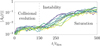 |
Fig. 1. Time evolution of the bisymmetric fluctuations (Equation B.6) in 12 different N–body realisations of the Mestel disc, with N = 25 × 106 particles each, using a running average over 30 dynamical times. The disc is initially stable and slowly relaxes towards an unstable state. Once unstable, the evolution is dominated by an exponentially growing mode before it saturates. The disc’s configuration is illustrated in Figure 2. Interestingly, the dispersion among realisations greatly increases close to the instability. The dashed line at t/tdyn = 150 is the time at which the changes in the DF are measured in Figure 3. |
 |
Fig. 2. Illustration of the typical evolution of a Mestel disc in one N–body simulation, via the surface density (up to R = 8R0) at two different times. During the collisional phase (left), the disc remains reasonably axisymmetric, displaying recurrent weak transient spirals. After the phase transition (right), the disc develops strong bisymmetric fluctuations, which ultimately saturate (Figure 1), up to the late formation of a bar (see Figure 10 in F+15). |
In Figure 1 we note that the dispersion among the different realisations gets much larger as the phase transition is approached. Heuristically, this increased scatter is caused by the fact that fluctuations get ever more amplified by collective effects, as the system nears the gravitational instability. During the phase transition, linear theory even predicts a divergence of the amplitude of fluctuations, a process sometimes called critical opalescence (see e.g. Chavanis 2023). In that case, Poisson fluctuations get larger, hence naturally driving a larger scatter among independent realisations. In practice, close to a phase transition, long-range interacting systems can even exhibit strange scaling in their finite-N fluctuations differing from simple Poisson statistics (see e.g. Yamaguchi 2016, for a detailed investigation in the context of the HMF model). Given the close similarities between stellar bar instability and the HMF (Lynden-Bell 1979; Rozier et al. 2019), it is likely that this strange scaling, not predicted by classical statistical mechanics, is responsible for the boosted dispersion observed during the unstable regime of Figure 1. This will be the topic of future work.
3.3. Ensemble-averaged relaxation rate
We now focus on the first stage of evolution and consider the averaged relaxation rate in action space, ∂F(J, t)/∂t, at the time t = 150 tdyn. This is what we present in Figure 3, one of the main result of the present work. In that figure we compare the BL prediction of the relaxation rate (top panel) with the ensemble-averaged relaxation rate measured in N–body simulations. As expected, we recover that the discs are heated up by resonant encounters, and the orbits diffuse from quasi-circular orbits to more eccentric ones. We find that the kinetic prediction and the N–body measurements are in quantitative agreement. The two approaches predict similar shapes for the relaxation rate in action space and, importantly, with similar amplitudes. Using the same criterion as in Equation (12) of Tep et al. (2022), we find that ∫dJ F |∂F/∂t| agrees within 10% between both panels. This is an important validation of BL.
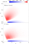 |
Fig. 3. Top: Local relaxation rate, ∂F/∂t, in action space as predicted by BL (Equation 3) for the Mestel disc (Section 2.1), computed in the centre of the action bins. The red regions correspond to an increase in the number of particles, while the blue contours correspond to a depletion. Bottom: Relaxation rate measured in N–body simulations of the same disc, averaged over 1 000 realisations with N = 25 × 106 particles each. The changes in the DF are computed at t/tdyn = 150, safely before the discs become unstable (Figure 1). The prediction and measurement are in good agreement, both in shape and amplitude. Slices in action space are illustrated in Figure 4. Collective effects play a crucial role in shaping the long-term evolution of razor-thin discs. |
In Figure 4 we present slices of Figure 3 through action space. These slices show that the qualitative agreement seen in Figure 3 is indeed quantitative. The amplitude of the BL predictions falls within the distribution of simulated relaxation rates. This figure also highlights the large spread in the relaxation rate already visible in Figure 1. Such an agreement between BL and N–body simulations was definitely not a given. Indeed, the present discs are close to being marginally stable. This corresponds to a dynamical regime where strong collective amplification via the contributions from damped modes may have a significant impact on long-term relaxation (see e.g. Hamilton & Heinemann 2020).
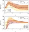 |
Fig. 4. Slices of the local relaxation rate, ∂F/∂t, from Figure 3 for fixed Jr (top) or fixed L (bottom), as predicted from BL (dashed) and measured in N–body simulations (full lines). Here, ∂F/∂t in the top (resp. bottom) panel has been averaged over an interval of width δJr = ± 0.02 (resp. δL = 0.06) and subsequently smoothed with a running average of width δL = 0.03 (resp. δJr = 0.01). For the N–body, we measured ∂F/∂t in each realisation independently, estimated the standard deviation among the sample of realisations, and represented the level lines one standard deviation away from the mean value. |
The diffusion captured by BL is quasi-linear in the sense that its derivation assumes that the system’s (small) finite-N fluctuations follow the disc’s unperturbed orbits (see e.g. Chavanis 2012). Since it is 2D and axisymmetric, the mean orbital structure of the present disc is fully regular. As such, BL does not encapsulate any relaxation driven by chaotic diffusion (see e.g. Lichtenberg & Lieberman 1983). The good agreement observed in Figure 3 between BL and the N-body measurements is a testimony to the fact that chaotic diffusion is weak here, at least before the onset of gravitational instability. In practice, this could have been expected since the present system is low-dimensional and weakly deviates from axial symmetry (see the left panel of Figure 2), therefore remaining close to integrability. As a result, the web of overlap between chaotic regions is bound to be limited, hence making chaotic diffusion quite inefficient (Lichtenberg & Lieberman 1983). Nevertheless, quantifying precisely the efficiency of such stochastic effects as relaxation proceeds would be a worthwhile future investigation.
After the onset of the gravitational instability, BL does not apply any longer. Nonetheless, in Appendix B.5, we repeat the N-body measurement from Figure 3 focusing there on longer timescales. We recover the boost in the relaxation rate close to instability, as well as large scatters among the independent realisations. We also find imprints, in action space, of resonant interactions between the disc’s strong non-axisymmetric perturbations and the bulk of the other stars.
4. Discussion
Following Figure 3, one could be tempted to conclude that BL effectively predicts the initial evolution of razor-thin self-gravitating discs, and to consider the matter settled. However, a closer examination reveals significant discrepancies between the results of S12, F+15, and our findings. Specifically, the timing of linear instability in Figure 1 and the shape of the flux in Figure 3 deserve further scrutiny. We note that the ensemble-averaged predictions as well as measurements from Figure 3 present rather broad signatures in action space. These differ from the sharp ridge-like features presented in the N–body simulation of S12 and the BL prediction from F+15. Furthermore, the overall amplitude of the flux is yet to be convincingly explained.
To explore these issues, we now address the questions of (i) the long-term impact of collective effects; (ii) the role that (weakly) damped modes play in this long-term evolution; (iii) whether softening has any long-term signatures; and (iv) the similarity of an individual disc to the ensemble average. We investigate these questions in order.
4.1. Neglecting collective effects
In dynamically hot systems, i.e. systems with large velocity dispersions, collective effects can be neglected. Then, BL reduces to the Landau equation (see Chavanis 2013, and references therein). As detailed in Appendix F, this amounts to replacing the dressed susceptibility coefficients,  , in Equation (3) with their bare counterpart, Ukk′. Figure 5 presents the relaxation rate in action space, as predicted by the inhomogeneous Landau equation. There are two main takeaways from this figure.
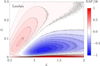 |
Fig. 5. Relaxation rate, ∂F/∂t, as predicted by the Landau equation (see Appendix F), using the same convention as in Figure 3. The Landau equation predicts a more isotropic diffusion. In addition, the relaxation time predicted by BL is three orders of magnitude shorter than that predicted by Landau: the collective amplification is instrumental. |
First, as already pointed out by F+15, the BL relaxation rate is larger than the Landau value by three orders of magnitude. Phrased differently, collective effects considerably accelerate the relaxation. In the present half-mass Mestel disc (Q = 1.5), Toomre (1981) has shown that collective effects can swing amplify (Goldreich & Lynden-Bell 1965; Julian & Toomre 1966) perturbations by a factor  (Figure 7 therein). Since BL involves the dressing squared, i.e.
  , this leads to a considerable acceleration of the relaxation. We obtain
  .
.
Second, we note that the BL relaxation rate (Figure 3) presents much sharper structures in action space compared to the Landau rate (Figure 5). However, both kinetic equations are inhomogeneous and account for resonant encounters. We argue that the narrower features predicted by BL stem from the imprint of the disc’s weakly damped modes. These modes drive strong localised responses in the disc. This is what we explore in the next section.
4.2. Weakly damped modes
To understand the role played by weakly damped modes we illustrate, in Figure 6, the BL relaxation rate in addition to the disc’s linear susceptibility. Figure 6 is an intricate figure, that we now describe carefully.
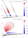 |
Fig. 6. Illustration of the connexion between a disc’s long-term relaxation and the disc’s linear damped modes. In each panel, we represent in the top plot the relaxation rate in action space, predicted by BL, using the same convention as in Figure 3. In the bottom plot, we represent the disc’s susceptibility, |N(ω)| (Equation C.6) represented at the circular angular momentum corresponding to their ILR (see Equation 4). The numerical saturation of the susceptibility for damped frequencies, γ < 0, is to be expected (see e.g. Appendix B in Petersen et al. 2024). Top: Prediction purposely using an insufficient number of basis elements (Appendix C.1) and too few resonances, for illustration purposes. In that case, the disc’s susceptibility contains three clear damped modes. These modes have a direct signature in the BL relaxation rate. The black line corresponds to the ILR resonance line associated with each mode, while the dashed lines correspond to the direction of diffusion. The proximity of these two lines enhances the efficiency of ILR for heating the disc. Bottom: Same as above, but using a numerically converged linear susceptibility, namely using the same parameters as in Figure 3. In both figures we show that the disc’s long-term heating is strongly enhanced at resonance with the underlying weakly damped modes. |
Figure 6 is composed of two panels, each of them with two sub-plots. In both panels, the top plot is the BL relaxation rate in action space, using the same convention as in Figure 3. The bottom plot represents the disc’s susceptibility, through the determinant of the susceptibility matrix, |N(ω)| (Equation C.6). A mode corresponds to a (complex) frequency, ω, such that |N(ω)| diverges, i.e. they appear as poles in this panel. However, here we do not represent the susceptibility in frequency space, but rather translate Re[ω] into an action through the circular angular momentum of the associated inner Lindblad resonance (ILR). More precisely, to any Re[ω], we can unambiguously associate an angular momentum, L, by solving
![Mathematical equation: $$ \begin{aligned} \mathbf{k }_{\mathrm{ILR} } \!\cdot \! {\boldsymbol{\Omega }} (J_{r} \!=\! 0 , L) = {\mathrm{Re} }[\omega ] , \end{aligned} $$](/articles/aa/full_html/2025/07/aa54102-25/aa54102-25-eq9.gif) (4)
(4)
with the resonance vector  . With this convention, if a quasi-circular orbit resonates with the mode through its ILR, then the location of the orbit in action space will lie just above the associated mode in the susceptibility plot.
In Figure 6, the two panels correspond to the same disc model, but use different calculations of the linear susceptibility. The top panel intentionally includes a reduced number of basis elements (Appendix C.1), and hence degrades the convergence of the linear predictions. This allows the physical processes at play here to appear more clearly. The bottom panel uses the same parameters as in Figure 3, with a much larger number of basis elements. It therefore relies on a converged estimation of the linear susceptibility.
We now focus on the top panel of Figure 6. In that degraded case, the linear calculation predicts (at least) three weakly damped modes. In the associated BL prediction, we note that each of these modes is at the origin of a sharp resonant ridge in action space. More precisely, the real part of the mode’s frequency dictates the position of the induced ridge in action: the larger the mode’s pattern speed, the further in the resonant ridge appears. The imaginary part of the mode’s frequency dictates the width of the induced ridge in action space: the faster the mode’s damping, the wider the imprint of the ridge in action space. Overall, we note that the resonant signatures of the damped modes, because they drive such a strong collective amplification, fully dominate the long-term relaxation predicted by BL.
The same mechanism is operating in the bottom panel of Figure 6. In this case, the disc’s linear susceptibility along the real axis is large within a broad frequency region, and does not display sharp signatures of distinguishable damped modes (given the shapes of the isocontours). This, in turn, drives significant amplification across a wide range of angular momenta, resulting in the broader heating in action space predicted by BL. As a consequence, BL does not exhibit distinct ridges in action space. Naturally, it would be highly valuable to refine our current implementation of linear response theory to overcome the numerical saturation evident in Figure 6 and gain a clearer understanding of the modal structure of the Mestel disc.
Orbits that resonate with a mode through their ILR flow in action space along the direction of kILR. Phrased differently, these orbits are heated towards more eccentric orbits with smaller guiding radii. It is worth noting that, coincidentally for the ILR, this direction of diffusion aligns closely with the associated resonance line, i.e. the line of constant kILR ⋅ Ω(J) (black line in the top panel of Figure 6). This alignment makes the ILR a particularly efficient resonance for heating the disc.
Interestingly, S12 observed the local power spectrum of fluctuations in their N–body simulations, before any instability has kicked in. Their resulting Figure 4 is reproduced here in Figure 7. In that figure, three peaks can be observed in the power spectrum, each corresponding to its respective ILR radius. These peaks are possibly associated with weakly damped modes excited by Poisson shot noise. While their number appears tentatively comparable to our results, any such comparison should be approached with caution. The prediction in the top panel of Figure 6 was degraded for illustration purposes. Obviously, improving the convergence of the linear predictions is necessary for more quantitative comparisons. In addition, one could also experiment with the method from Weinberg (1994), Heggie et al. (2020) to track damped modes in N–body simulations.
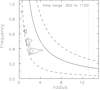 |
Fig. 7. Figure from S12. Power spectra of the ℓ = 2 fluctuations as a function of radius in their N–body simulation. The presence of three peaks in these early power spectra, and their location at their respective ILR, is likely the resonant signature of weakly damped modes. |
Finally, we briefly comment on the difference between the BL prediction from F+15 (Figure 4 therein) and our current BL prediction (Figure 3). In F+15, BL predicted a single sharp ridge in action space, whereas in the present work BL predicts broader heating in action space. Since the prediction from BL is closely tied to the accuracy of the linear susceptibility, the discrepancy between these two studies stems from the computation of the dressed coupling coefficients,  , which were badly converged in F+15. Appendix E details the improved methodology used in the present work to compute these coefficients more accurately.
4.3. Impact of softening
In Appendix G, following De Rijcke et al. (2019b), we investigate how softening affects the complex frequency of growing modes in an unstable disc. In particular, in Figure G.1, we show that Plummer softening (Equation G.2) tends to shift unstable modes towards a lower pattern speed and lower growth rate. As a consequence, if the same trend also applies to damped modes, we expect that the stronger the softening, the faster the damping of the modes. Rephrased using the insight from Figure 6, we expect that when the softening is stronger, (i) the action space ridges should appear later and (ii) these ridges would move towards higher angular momenta. We set out to investigate these trends in N–body simulations.
In Figure 8, we illustrate the long-term evolution of bisymmetric fluctuations in N–body simulations for the two softening kernels presented in Appendix G with different values of the softening length, ε. In that figure, it is clear for the Plummer softening kernel that increasing ε delays the phase transition towards instability. We claim that this is so because softening affects the collisionless properties of the disc, and consequently its collisional dressed resonant relaxation. Phrased differently, Plummer softening makes the disc more linearly stable than it should be. Consequently, softening reduces swing amplification and ultimately delays relaxation4.
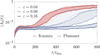 |
Fig. 8. Same as Figure 1, but for various softening lengths, ε, and two different softening kernels (Appendix G). The level of transparency corresponds to different softening lengths (Equation G.1) with the bottom (resp. top) line corresponding to 20% (resp. 80%) contours over 100 independent realisations with N = 25 × 106 particles. The case Kuzmin ε = 0.16 corresponds to Figure 1. For the Plummer kernel, the larger the softening length, the slower the relaxation, and the more delayed the transition to instability. This kernel introduces a strong gravitational bias when compared with non-softened theoretical predictions (Figure G.1). On the contrary, simulations using the Kuzmin kernel behave similarly across softening lengths. Interestingly, we note that, in every case, the dispersion among realisations increases near phase transition. |
The trend from Figure 8 also explains the difference in the time of phase transition between the simulation of S12 and ours. In Figure 2 of S12, the instability sets in at t ≃ 1 200 tdyn using the Plummer softening with ε = 0.125 and N = 50 × 106. In our case (Figure 8), using N = 25 × 106, the instability sets in at t ≃ 400 tdyn (resp. 800) for the Plummer softening with ε ≃ 0.08 (resp. 0.16). Once accounting for the rescaling by the factor 1/N, these timescales are nicely consistent.
We conclude this section by emphasising the importance of accounting for the bias introduced by softening when comparing N–body simulations with linear response and kinetic theory that both assume the (non-softened) Newtonian pairwise interaction. In Figure 3, we carefully chose a softening kernel, namely Kuzmin softening (Equation G.3), so that the corresponding bias is small. This kernel affects much less the disc’s linear response (see Figure G.1), so that varying the softening length does not bias as much their long-term relaxation compared to the case of the (non-softened) Newtonian interaction (Figure 8).
4.4. Long-term stochasticity
BL predicts the ensemble-averaged evolution, i.e. averaged over different initial conditions drawn from the same DF. It is also of interest to investigate the dispersion that may exist among different realisations of the same disc. To do so, we represent in Figure 9 the relaxation rate measured in 12 independent simulations whose fluctuations are presented in Figure 1.
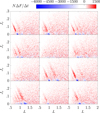 |
Fig. 9. Relaxation rate, ∂F/∂t, measured in 12 independent N–body realisations, using the same convention as in Figure 3. The number, location, amplitude, and birth time of the action ridges vary strongly from one realisation to another. This is a measure of a long-term stochasticity in the vicinity of the phase transition (see also Figure 4). |
In Figure 9, we note that individual realisations are very different from the averaged one (Figure 3). In the ensemble-averaged figure, all the circular orbits (0.75 ≲ L ≲ 1.5) are depopulated while more eccentric orbits get further populated. However, in individual realisations, the changes in the DF are much more localised and concentrated along one or multiple sharp ridges in action space. These ridges come in different number, locations, and at different time and amplitude in each realisation5. We note that their individual intensity is up to 2–3 times higher than the averaged value. In Figure B.2, we present the standard deviation of the relaxation rate over the independent realisations; we also recover the renewal of stochasticity near marginal stability.
BL is, by design, unable to predict such a diversity. Predicting the scatter among realisations could be addressed within the context of the theory of large deviations (see e.g. Feliachi & Bouchet 2022). However, the inclusion of collective effects in this context is still an open question (Feliachi & Fouvry 2024). As such, the details of the processes responsible for this long-term stochasticity are still to be understood.
5. Conclusion
We presented applications of the BL kinetic theory to the self-induced long-term evolution of razor-thin self-gravitating discs. We showed that the inhomogeneous BL Equation (3) is able to quantitatively predict the mean long-term evolution of these systems up to the onset of gravitational instability. The kinetic predictions were successfully compared with N–body simulations averaged over many realisations (Figure 3). Doing so, we highlighted the importance of resonant encounters and collective effects in driving the relaxation of stellar discs. The consequences of self-gravity proved to be particularly diverse (Figure 5) and would have been difficult to predict a priori without the valuable insights provided by BL.
In these marginally stable systems, fluctuations are strongly swing amplified by resonating with the disc’s underlying weakly damped modes (Figure 6). The disc’s long-term evolution is therefore particularly sensitive to the collisionless linear response of the disc. By stabilising the disc, we showed that softening delays the phase transition to instability (Figure 8). We also showed that the choice of softening kernel was critical when compared with non-softened theoretical predictions. In that view, the Plummer softening, when used to simulate razor-thin discs, introduces a much larger bias than the Kuzmin softening. Finally, we noted that, in this regime, the average relaxation rate is not representative of the individual realisations. As the disc nears marginal stability, the variance among realisations becomes increasingly large (Figure 9). In that sense, the average cold galaxy does not exist. We conclude with a few prospects worth exploring to further our theoretical understanding of the long-term evolution of self-gravitating discs.
-
Small scales versus large scales – BL diverges on small scales (see e.g. Chavanis 2013). Chandrasekhar (1943) did regularise the deflections on small scales, and took hard encounters into account. This regularisation should be adapted to the resonant kinetic theories (see e.g. Fouvry et al. 2021), therefore weighing the respective impact of small versus large scales on long-term relaxation. In (cold) razor-thin galactic discs, the long-range dressing by collective effects is likely to dominate, but this remains to be accurately quantified.
-
Time evolution – A direct follow-up of this work would involve integrating BL forward in time, beyond the onset of relaxation. However, integrating these equations is challenging (Weinberg 2001). There are two main difficulties to overcome: computing the resonant diffusion coefficients and determining the self-consistent potential (and actions) as the disc evolves. One potential approach is to integrate the corresponding stochastic Langevin equation (see e.g. Hénon 1971; Cohn 1979; Giersz 1998; Fu et al. 2025). This could ultimately serve to validate N–body codes on longer timescales.
-
Crossing marginal stability – BL unrealistically diverges at marginal stability (Weinberg 1993), though we showed here that BL is still accurate relatively close to the phase transition. However, if one were to evolve BL in time, it would inevitably break at some point. This divergence must be regularised by considering mode-particle interactions, in the spirit of the so-called quasi-linear theory in plasma physics (see e.g. Rogister & Oberman 1968; Hamilton & Heinemann 2020, 2023).
-
Non-linear regime – After the phase transition, the disc’s evolution is dominated by the emerging unstable mode. As this mode grows, non-linear contributions become increasingly important, up to the point of saturation and trapping at resonances (see e.g. Hamilton 2024). Investigating this late-time non-linear regime is an interesting venue.
-
Beyond average predictions – As highlighted in Figure 9, near marginal stability the variance among different realisations increases tremendously. Predicting this scatter is crucial to assess the likelihood of a given realisation. This is beyond the reach of BL, but the theory of large deviations offers promising perspectives (see e.g. Bouchet 2020; Feliachi & Bouchet 2022; Feliachi & Fouvry 2024). Ultimately, this should pave the way for the comparison of theoretical predictions of the scatter with observations andcosmological simulations.
-
Thick discs – The models studied here are not perfect representation of genuine galactic discs. While the case of spherically symmetric systems is well captured by BL (Rozier et al. 2019; Fouvry et al. 2021; Tep et al. 2022), the extension to thick discs or flattened spheres is yet to be achieved beyond the WKB approximation (Fouvry et al. 2017). One of the potential issues in these systems is the possible lack of integrability (see e.g. Weinberg 2015) beyond the Stäckel family (Tep et al. 2024).
-
Coupled halo-disc evolution – We assumed that the disc was embedded within a static, rigid dark matter halo. However, the dark matter halo, albeit dynamically hotter, is also subject to fluctuations. Accounting for the coupling between the disc and the halo should provide a more realistic picture of the long-term evolution of galaxies (see e.g. Johnson et al. 2023).
-
Impact of morphological type – The present analysis focused on the Mestel disc. It would be of interest to study the efficiency of orbital diffusion on more realistic exponential disc models (see e.g. De Rijcke et al. 2019a), for example while varying the bulge to disc mass, when scanning late galaxy types of the Hubble sequence (Reddish et al. 2022).
-
Open dissipative systems – Finally, galaxies are not isolated objects. The Milky Way for instance is continuously perturbed by external sources triggering various response features (see e.g. Grion Filho et al. 2021, for a review) that operate concurrently in open systems. In addition, the accounting of dissipative processes within the baryonic component can drive unlikely evolutionary pathways, possibly leading to self-regulation (Pichon 2023). This should also be the topic of future work.
Data availability
The data underlying this article are available through reasonable request to the author. The code for the diffusion coefficient, written in julia (Bezanson et al. 2017), is available online6. The N–body code (courtesy of John Magorrian) is also publicly available7.
Here we refer to the discs as cold to emphasise that their small, but non-zero, velocity dispersion causes them to support strong linear amplification (Toomre 1964). These should not be confused with infinitely cold discs, i.e. discs with exactly zero velocity dispersion (see e.g. Erickson 1974; Miller 1974).
To ease the numerics, we soften Equation (1) with  , with ϵ ≪ 1. We checked that this softening had no impact on our predictions.
In both cases the initial conditions were from a quiet start (Debattista & Sellwood 2000; Sellwood 2024). It would be interesting to investigate whether such non-Poisson-like initial conditions can bias the disc’s long-term relaxation.
The same trend with softening would also happen if the disc’s relaxation were driven by two-body local encounters (Theis 1998). However, such local contributions are absent from our experiments since our simulations are, by design, limited to ℓ = 2 fluctuations.
S12 and F+15 focused on a single realisation and did not perform any ensemble average.
As in F+15, we interpret this constraint as ‘no particles with orbits that extend beyond Rmax’, i.e. F(E, L) = 0 when E > ψeff(Rmax), and not ψ(Rmax) (see S12).
For example, we checked that using the same control parameters as F+15 within LinearResponse.jl (Petersen et al. 2024) leads to the incorrect prediction that the half-mass Mestel disc is unstable.
This kernel mimics the effect of finite thickness (Sellwood 2014).
Acknowledgments
This work is partially supported by grant Segal ANR-19-CE31-0017 of the French Agence Nationale de la Recherche, by the Idex Sorbonne Université, and in part by grant NSF PHY-2309135 to the Kavli Institute for Theoretical Physics (KITP). We are grateful to J. Barré, E. Donghia, S. Flores, E. Ko, J. Magorrian, M. Petersen, K. Tep, and M. Weinberg for constructive comments. We thank J. Magorrian for providing us with his code, and Stéphane Rouberol for the smooth running of the Infinity cluster, where the simulations were performed.
References
- Aarseth, S. J. 1963, MNRAS, 126, 223 [NASA ADS] [Google Scholar]
- Benetti, F. P. C., & Marcos, B. 2017, Phys. Rev. E, 95, 022111 [Google Scholar]
- Bezanson, J., Edelman, A., Karpinski, S., & Shah, V. B. 2017, SIAM Rev., 59, 65 [Google Scholar]
- Binney, J., & Tremaine, S. 2008, Galactic Dynamics, 2nd edn. (Princeton Univ Press) [Google Scholar]
- Bouchet, F. 2020, J. Stat. Phys., 181, 515 [Google Scholar]
- Campa, A., Chavanis, P.-H., Giansanti, A., & Morelli, G. 2008, Phys. Rev. E, 78, 040102 [Google Scholar]
- Chakrabarty, D. 2004, MNRAS, 352, 427 [Google Scholar]
- Chandrasekhar, S. 1943, ApJ, 97, 255 [Google Scholar]
- Chavanis, P.-H. 2012, Phys. A, 391, 3680 [CrossRef] [MathSciNet] [Google Scholar]
- Chavanis, P.-H. 2013, A&A, 556, A93 [NASA ADS] [CrossRef] [EDP Sciences] [Google Scholar]
- Chavanis, P.-H. 2023, Universe, 9, 68 [Google Scholar]
- Chavanis, P.-H. 2024, Eur. Phys. J. Plus, 139, 51 [Google Scholar]
- Clutton-Brock, M. 1972, Ap&SS, 16, 101 [NASA ADS] [CrossRef] [Google Scholar]
- Cohn, H. 1979, ApJ, 234, 1036 [NASA ADS] [CrossRef] [Google Scholar]
- Debattista, V. P., & Sellwood, J. A. 2000, ApJ, 543, 704 [Google Scholar]
- Dehnen, W. 2001, MNRAS, 324, 273 [NASA ADS] [CrossRef] [Google Scholar]
- De Rijcke, S., Fouvry, J.-B., & Pichon, C. 2019a, MNRAS, 484, 3198 [Google Scholar]
- De Rijcke, S., Fouvry, J.-B., & Dehnen, W. 2019b, MNRAS, 485, 150 [Google Scholar]
- Earn, D. J. D., & Sellwood, J. A. 1995, ApJ, 451, 533 [Google Scholar]
- Eilers, A.-C., Hogg, D. W., Rix, H.-W., & Ness, M. K. 2019, ApJ, 871, 120 [Google Scholar]
- Erickson, Jr., S. A. 1974, Ph.D. Thesis, Massachusetts Institute of Technology, USA [Google Scholar]
- Evans, N. W., & Read, J. C. A. 1998, MNRAS, 300, 106 [Google Scholar]
- Feliachi, O., & Bouchet, F. 2022, J. Stat. Phys., 186, 22 [Google Scholar]
- Feliachi, O., & Fouvry, J.-B. 2024, Phys. Rev. E, 110, 024108 [Google Scholar]
- Fouvry, J.-B., & Bar-Or, B. 2018, MNRAS, 481, 4566 [Google Scholar]
- Fouvry, J.-B., & Prunet, S. 2022, MNRAS, 509, 2443 [NASA ADS] [Google Scholar]
- Fouvry, J.-B., Pichon, C., Magorrian, J., & Chavanis, P.-H. 2015, A&A, 584, A129 [NASA ADS] [CrossRef] [EDP Sciences] [Google Scholar]
- Fouvry, J.-B., Pichon, C., Chavanis, P.-H., & Monk, L. 2017, MNRAS, 471, 2642 [Google Scholar]
- Fouvry, J.-B., Hamilton, C., Rozier, S., & Pichon, C. 2021, MNRAS, 508, 2210 [CrossRef] [Google Scholar]
- Fu, Y., Angus, J. R., Qin, H., & Geyko, V. I. 2025, Phys. Rev. E, 111, 025211 [Google Scholar]
- Gaia Collaboration 2016, A&A, 595, A2 [NASA ADS] [CrossRef] [EDP Sciences] [Google Scholar]
- Gardner, J. P., Mather, J. C., et al. 2006, Space Sci. Rev., 123, 485 [Google Scholar]
- Giersz, M. 1998, MNRAS, 298, 1239 [NASA ADS] [CrossRef] [Google Scholar]
- Goldreich, P., & Lynden-Bell, D. 1965, MNRAS, 130, 125 [Google Scholar]
- Grion Filho, D., Johnston, K. V., Poggio, E., et al. 2021, MNRAS, 507, 2825 [NASA ADS] [CrossRef] [Google Scholar]
- Hamilton, C. 2024, MNRAS, 528, 5286 [Google Scholar]
- Hamilton, C., & Heinemann, T. 2020, ArXiv e-prints [arXiv: 2011.14812] [Google Scholar]
- Hamilton, C., & Heinemann, T. 2023, MNRAS, 525, 4161 [Google Scholar]
- Heggie, D. C., Breen, P. G., & Varri, A. L. 2020, MNRAS, 492, 6019 [Google Scholar]
- Hénon, M. 1971, Ap&SS, 14, 151 [NASA ADS] [CrossRef] [Google Scholar]
- Hernquist, L., & Ostriker, J. P. 1992, ApJ, 386, 375 [Google Scholar]
- Heyvaerts, J. 2010, MNRAS, 407, 355 [NASA ADS] [CrossRef] [Google Scholar]
- Hunt, J. A. S., Bub, M. W., Bovy, J., et al. 2019, MNRAS, 490, 1026 [NASA ADS] [CrossRef] [Google Scholar]
- Johnson, A. C., Petersen, M. S., Johnston, K. V., & Weinberg, M. D. 2023, MNRAS, 521, 1757 [CrossRef] [Google Scholar]
- Julian, W. H., & Toomre, A. 1966, ApJ, 146, 810 [NASA ADS] [CrossRef] [Google Scholar]
- Kalnajs, A. J. 1976, ApJ, 205, 745 [CrossRef] [Google Scholar]
- Kuhn, V., Guo, Y., Martin, A., et al. 2024, ApJ, 968, L15 [NASA ADS] [CrossRef] [Google Scholar]
- Lichtenberg, A. J., & Lieberman, M. A. 1983, Regular and stochastic motion (Springer) [CrossRef] [Google Scholar]
- Lynden-Bell, D. 1979, MNRAS, 187, 101 [Google Scholar]
- Lynden-Bell, D., & Kalnajs, A. J. 1972, MNRAS, 157, 1 [Google Scholar]
- Magorrian, J. 2007, MNRAS, 381, 1663 [Google Scholar]
- Merritt, D. 1996, AJ, 111, 2462 [Google Scholar]
- Mestel, L. 1963, MNRAS, 126, 553 [NASA ADS] [CrossRef] [Google Scholar]
- Miller, R. H. 1971, Ap&SS, 14, 73 [Google Scholar]
- Miller, R. H. 1974, ApJ, 190, 539 [Google Scholar]
- Petersen, M. S., Roule, M., Fouvry, J.-B., Pichon, C., & Tep, K. 2024, MNRAS, 530, 4378 [Google Scholar]
- Pichon, C. 2023, KITP (Santa Barbara), https://doi.org/10.26081/K6BD50 [Google Scholar]
- Polyachenko, E. V. 2013, Astro. Lett., 39, 72 [Google Scholar]
- Reddish, J., Kraljic, K., Petersen, M. S., et al. 2022, MNRAS, 512, 160 [NASA ADS] [CrossRef] [Google Scholar]
- Rogister, A., & Oberman, C. 1968, J. Plasma Phys., 2, 33 [Google Scholar]
- Romeo, A. B. 1994, A&A, 286, 799 [NASA ADS] [Google Scholar]
- Romeo, A. B. 1997, A&A, 324, 523 [NASA ADS] [Google Scholar]
- Romeo, A. B. 1998, A&A, 335, 922 [Google Scholar]
- Roule, M., Fouvry, J.-B., Pichon, C., & Chavanis, P.-H. 2022, Phys. Rev. E, 106, 044118 [Google Scholar]
- Rozier, S., Fouvry, J. B., Breen, P. G., et al. 2019, MNRAS, 487, 711 [CrossRef] [Google Scholar]
- Rybicki, G. B. 1972, in Gravitational N-Body Problem, ed. M. Lecar, 31, 22 [Google Scholar]
- Salo, H., & Laurikainen, E. 2000, MNRAS, 319, 393 [NASA ADS] [Google Scholar]
- Sellwood, J. A. 2012, ApJ, 751, 44 [NASA ADS] [CrossRef] [Google Scholar]
- Sellwood, J. A. 2014, Rev. Mod. Phys., 86, 1 [Google Scholar]
- Sellwood, J. A. 2020, MNRAS, 492, 3103 [Google Scholar]
- Sellwood, J. A. 2024, MNRAS, 529, 3035 [Google Scholar]
- Sellwood, J. A., & Binney, J. J. 2002, MNRAS, 336, 785 [Google Scholar]
- Sellwood, J. A., & Evans, N. W. 2001, ApJ, 546, 176 [NASA ADS] [CrossRef] [Google Scholar]
- Sellwood, J. A., & Kahn, F. D. 1991, MNRAS, 250, 278 [NASA ADS] [Google Scholar]
- Sun, W., Shen, H., Jiang, B., & Liu, X. 2025, ApJ, 979, 103 [Google Scholar]
- Tep, K., Fouvry, J.-B., & Pichon, C. 2022, MNRAS, 514, 875 [CrossRef] [Google Scholar]
- Tep, K., Pichon, C., & Petersen, M. S. 2024, ArXiv e-prints [arXiv:2412.15033] [Google Scholar]
- Theis, C. 1998, A&A, 330, 1180 [Google Scholar]
- Toomre, A. 1964, ApJ, 139, 1217 [Google Scholar]
- Toomre, A. 1981, Structure and Evolution of Normal Galaxies, 111 [Google Scholar]
- Tremaine, S., & Weinberg, M. D. 1984, MNRAS, 209, 729 [Google Scholar]
- Trick, W. H., Coronado, J., & Rix, H.-W. 2019, MNRAS, 484, 3291 [NASA ADS] [CrossRef] [Google Scholar]
- Weinberg, M. D. 1993, ApJ, 410, 543 [Google Scholar]
- Weinberg, M. D. 1994, ApJ, 421, 481 [NASA ADS] [CrossRef] [Google Scholar]
- Weinberg, M. D. 2001, MNRAS, 328, 311 [Google Scholar]
- Weinberg, M. D. 2015, ArXiv e-prints [arXiv:1508.06855] [Google Scholar]
- White, R. L. 1988, ApJ, 330, 26 [Google Scholar]
- Yamaguchi, Y. Y. 2016, Phys. Rev. E, 94, 012133 [Google Scholar]
- Yu, J., & Liu, C. 2018, MNRAS, 475, 1093 [Google Scholar]
- Zang, T. A. 1976, Ph.D. Thesis, Massachusetts Institute of Technology, USA [Google Scholar]
Appendix A: Razor-thin disc
A.1. Angle-action coordinates
Axisymmetric razor-thin discs are integrable, i.e. appropriate angle-action coordinates can explicitly be constructed for them (Lynden-Bell & Kalnajs 1972). In practice, we follow the same approach as in the library OrbitalElements.jl, whose main conventions we recall here (see Appendix A1 in PR+24).
Orbits in a razor-thin disc can be equivalently labelled by their energy and angular momentum, (E, L), their action (Jr, L) – with Jr the radial action, or with their pericentre and apocentre, (rp, ra) (see Equations A1–A3 in PR+24). Orbits are skimmed with frequencies (Ωr, Ωϕ) = (αΩ0, αβΩ0), with Ω0 some frequency scale. The frequency ratios (α, β) readily follow from the angle-action mapping (see Equation A4 in PR+24). Following Appendix A1.1 in PR+24, all angular integrals are performed using the so-called Hénon anomaly, with additional interpolations to handle extreme orbits, e.g. exactly circular or radial orbits.
A.2. Distribution function
The DF of the Mestel disc from Equation (2) satisfies (Equation 4.163 in Binney & Tremaine 2008)
![Mathematical equation: $$ \begin{aligned} q \!=\! \bigg ( \frac{V_0}{\sigma } \bigg )^2 \!\!-\! 1 , \,\, C \!=\! \frac{V_0^2}{2^{q/2+1}\pi ^{3/2}\,G\;\Gamma [\tfrac{q+1}{2}] \sigma ^{q+2}R_0^{q+1}} . \end{aligned} $$](/articles/aa/full_html/2025/07/aa54102-25/aa54102-25-eq13.gif) (A.1)
(A.1)
In order to deal with the central singularity and the disc’s infinite mass, we follow Evans & Read (1998) and introduce an inner and outer tapering in the DF, leaving the mean potential unchanged. The total potential is then generated by (i) an inert bulge, (ii) an inert halo, and (iii) the self-gravitating disc. In addition, one may vary the overall amplitude of the DF with the active fraction ξ. This acts as a proxy for the relative masses of the disc and its surrounding halo. The disc’s DF reads
 (A.2)
(A.2)
In this equation, the tapers read
 (A.3)
(A.3)
The sharpness of the inner (resp. outer) taper is controlled by the power index ν (resp. μ), while its location is set by the radius Rin (resp. Rout). The outer taper was introduced by Evans & Read (1998), and is mandatory in N–body simulations to ensure that the disc is of finite mass.
The exact set of parameters we used are the same as in S12 and F+15. More precisely, in Figure 3, we take G = R0 = V0 = 1 and use these units throughout the paper. We also imposed ξ = 0.5 (half-mass disc), ϵ = 10−5 for the potential truncation (see footnote 2), and fixed the tapers to Rin = 1, Rout = 11.5, μ = 5, and ν = 4. Finally, we set the disc’s velocity dispersion to q = 11.4. The value of q slightly differs between S12 (q = 11.44) and F+15 (q = 11.4). In practice, this only changes the velocity dispersion by 0.1% and we checked that it did not impact our predictions. The value from S12 had a simple motivation: having nominal Toomre’s factor Q = 1.5.
Appendix B: N–body simulations
To perform our N–body simulation, we adapted the particle-mesh code used in F+15 (courtesy of John Magorrian), a simpler 2D version of the GROMMET code (Magorrian 2007). We refer to Section 5.1 of F+15 for a detailed description of the code. The N–body code (courtesy of John Magorrian) is publicly available8.
B.1. Sampling
Improving upon Appendix E of F+15, we sample the DF from (A.2) in (rp, ra)–space rather than in (E, L)–space. We briefly detail our approach.
Following Equation (A.2), we need to sample the DF
 (B.1)
(B.1)
complemented with the truncation constraint9
 (B.2)
(B.2)
In Equation (B.1), the constant Csp ensures that Fsp is normalised to unity when integrated with respect to dxdv. We report the values used in table B.1.
Sampling of the DFs from Equation (B.1).
The constraint from Equation (B.2) imposes that the populated domain in the (rp, ra)–space is a triangle. Accounting carefully for the Jacobian of the transformation (Jr, L) → (rp, ra), the density of state in (rp, ra) is
 (B.3)
(B.3)
where the (2π)2 factor comes from integrating over the angles, and the Jacobian |∂(E, L)/∂(rp, ra)| is computed using OrbitalElements.jl (PR+24).
To sample p(rp, ra), we use a rejection sampling against the uniform distribution
with the rejection constant M satisfying
 (B.4)
(B.4)
The values used for this rejection constant are given in table B.1.
B.2. Measuring fluctuations and modes
We now describe our method to measure the fluctuation’s strength (Figures 1 and 8) and to estimate the frequency and growth rate of the dominant mode in N–body simulations of unstable discs (Appendix G). We follow an approach similar to Appendix C in F+15.
Considering that the system’s density fluctuations are well described by a single dominant mode, they read
 (B.5)
(B.5)
with ρM the shape of the mode and ωM its (complex) frequency. The density fluctuation can be projected on any spatial function, f(r) = f(r) eiℓϕ, to give
![Mathematical equation: $$ \begin{aligned} A_\ell (t) = \!\!\int \!\! {\mathrm{d} } \mathbf{r } f(\mathbf{r }) \, \delta \rho (\mathbf{r },t) = m \sum _{i = 1}^{N} f[r_i(t)] \, {\mathrm{e} }^{{\mathrm{i} }\ell \phi _i(t)}, \end{aligned} $$](/articles/aa/full_html/2025/07/aa54102-25/aa54102-25-eq22.gif) (B.6)
(B.6)
From the time series t → Aℓ(t), one expects then the behaviour
![Mathematical equation: $$ \begin{aligned} |A_\ell (t)| \propto {\mathrm{e} }^{{\gamma _{{m }}} t}; \quad \arg [A_\ell (t)] \propto {\Omega _{{m }}} t , \end{aligned} $$](/articles/aa/full_html/2025/07/aa54102-25/aa54102-25-eq23.gif) (B.7)
(B.7)
provided one unwraps the phases. In Figure B.1, we illustrate such time series for an unstable Mestel disc (namely, Zang’s ν = 4 disc, Zang 1976).
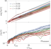 |
Fig. B.1. Time series of the unwrapped phase (top) and the norm (bottom) of the bisymmetric fluctuations probed by A2(t) from Equation (B.6) over ten independent realisations of the unstable Zang ν = 4 disc (Zang 1976). Each simulation is performed with N = 2 × 10⁸ particles using the Plummer softening kernel (Equation G.2) and for varying softening lengths, ε. For each ε, the same ten initial conditions are used and shown in the same colour. The frequency ΩM (resp. growth rate γM) of the mode are estimated by a linear fit of the phase (resp. log of the norm) of such time series, only using t ≥ Tmin = 10 tdyn. The growth of the phase is generically more regular than the growth of the norm. The Plummer softening kernel introduces a strong gravity bias when compared with (non-softened) theoretical predictions. |
To measure the dominant mode’s frequency, we use the log-normal function
![Mathematical equation: $$ \begin{aligned} f(r) = \exp \!\left[-\frac{\ln (r/R_0)^2}{2\sigma ^2}\right], \end{aligned} $$](/articles/aa/full_html/2025/07/aa54102-25/aa54102-25-eq24.gif) (B.8)
(B.8)
with r0 = 1.33 and σ = 0.45. This mimics the radial shape of the mode, hence easing the measurement. If one uses multiple functions for the projections, one could also estimate the mode’s shape.
To investigate the long-term evolution of fluctuations in Figures 1 and 8, we use the simpler identity function
 (B.9)
(B.9)
with (rmin, rmax) = (1.5 r0, 4.5 r0). This removes the contributions from the disc’s central and outer regions, where very few particles are present.
B.3. Measuring the relaxation rate
To measure the BL relaxation rate in numerical simulations (Figure 3), we performed 1 000 realisations of the Mestel disc, each with N = 25 × 106 particles. We used the Kuzmin softening (Equation G.3) with ε = 0.16 sufficiently small so that the gravitational bias is negligible with respect to non-softened theoretical predictions (see Figure G.1). For the numerical integration, we used a leapfrog scheme with timestep δt = 10−2 tdyn. The forces are estimated using a Cartesian grid that extends to ±xmax = 20 with nx × ny = 1 0242 cells. The ℓ = 2 fluctuations are selected using the same method as in Section 5.1 of F+15, with a polar grid of nr = 8 192 radial rings and nϕ = 2 048 points in the azimuthal direction.
For post-processing, we use OrbitalElements.jl to compute the particles’ actions (Jr, L) within the mean potential from Equation (1). We count their number, n(Ji, Lj), in bins of width δJr = 1/300, δL = 1/100. From these bin counts, the DF and its changes are obtained through
 (B.10)
where the (2π)2 prefactor comes from the integration over dθrdθϕ. To estimate ∂F/∂t in Figure 3, we computed the difference between t = 150 tdyn and t = 0.
In Figure B.2, we present the same measurement as in Figure 3, but focusing on the standard deviation of the local relaxation rate among the different realisations.
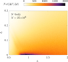 |
Fig. B.2. Same as in the bottom panel of Figure 3, but presenting here the standard deviation of the local relaxation rate, Nσ(∂F/∂t), over the available realisations. The scatter among different realisations is particularly significant, when compared with the average amplitude from Figure 3. |
In that figure, we find that, close to the region where the ridges form, the dispersion among realisations is of similar order than the average relaxation rate itself (Figure 3). This is the imprint of the resurgence of stochasticity near marginal stability, as also visible in Figure 9.
B.4. Convergence
In order to check the appropriate (statistical) convergence of the numerical measurements, in Figure B.3, we present the same measurement as in Figure 3 but varying the control parameters of the N-body code. More precisely, using the exact same measurement protocol in both figures, we either halved the integration timestep, δt, halved the softening length, ε, or doubled the sizes of the code’s various grids, via nx, nr, and nϕ. In Figure B.3, we find that the measurements of the averaged relaxation rate all agree with one another: this is a reassuring check.
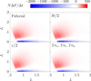 |
Fig. B.3. Same as in the bottom panel of Figure 3. Compared to the fiducial run (top left), we either halved the integration timestep (top right); halved the softening length (bottom left); or doubled the sizes of the Cartesian, radial, and azimuthal grids (bottom right). In all cases, the measurements of the local relaxation rate are fully consistent with one another. Here, the use of the Kuzmin softening kernel (Appendix G) is instrumental to obtain consistent results over a wide range of softening lengths (see Section 4.3). |
In Figure B.4, we repeat the same experiment, this time focusing on a single realisation. All measurements agree with one another. This strengthens our confidence in the appropriate convergence of the numerical integration.
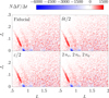 |
Fig. B.4. Same as Figure B.3 but, here, focusing on a single realisation. The structures of the relaxation rate in action space are all consistent with one another. |
B.5. Long-term relaxation
In this appendix, we use N-body simulations to briefly explore the long-term evolution of the discs as they undergo their dynamical transition towards instability (see Figure 1).
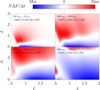 |
Fig. B.5. Same as in the bottom panel of Figure 3, but focusing here on later times, i.e. beyond the disc’s initial slow collisional evolution (Figure 1). The rate of change of the DF is estimated through simple time differences, as indicated in each panel. In each panel, the colours are rescaled to the minimum and maximum value of the local relaxation rate in that panel, as indicated therein. For simplicity, even at late times, actions remain evaluated within the disc’s initial unperturbed axisymmetric potential from Equation (1). |
This is first illustrated in Figure B.5, where we focus on the ensemble-averaged relaxation rate. One can make a few remarks from that figure: (i) Near the dynamical phase transition, i.e. for 150 tdyn ≤ t ≤ 450 tdyn (see Figure 3), the amplitude of the relaxation rate is greatly magnified. (ii) At all times, diffusion typically leads to the dynamical heating of quasi-circular orbits towards more eccentric ones. (iii) Finally, although here we are looking at relaxation within the disc’s initial axisymmetric angle-action coordinates, one should recall that during such late stages of relaxation, the disc contains strong non-axisymmetric perturbations, as visible in Figure 2, possibly trapping particles at resonance (see e.g. Tremaine & Weinberg 1984).
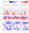 |
Fig. B.6. Same as Figure B.5, focusing here on three independent realisations (different columns). The structures of the diffusion in action space differ widely between realisations. Stochasticity is significantly enhanced during the disc’s dynamical phase transition throughinstability. |
In Figure B.6, we repeat the same measurement as in Figure B.5, this time focusing on three independent realisations. For each realisation, we typically find the same signatures as in the ensemble-averaged measurement from Figure B.5, although the diversity and scatter among the different realisations is very significant. Finally, at late times, i.e. within the non-linear regime, we note sharp resonant ridges in action space. These are caused by the resonant interactions between the disc’s non-axisymmetric perturbations (Figure 2) and the rest of the stars (see e.g. Sellwood & Kahn 1991).
Appendix C: Linear response theory
As shown in Equation (3), collective effects play a critical role in shaping the long-term relaxation of dynamically cold systems. Therefore, it is essential to handle the numerical aspects of linear response theory with precision. To do so, we use the publicly available library LinearResponse.jl (PR+24) and its associated dependencies. In this section, we briefly outline the main building blocks of this calculation.
C.1. Biorthogonal bases
Following the convention from AstroBasis.jl (PR+24), we introduce a basis of potential-density pairs
 (C.1)
(C.1)
 (C.2)
(C.2)
with U = − G/|r − r′| the gravitational potential. From these basis elements, the interaction potential takes the pseudo-separable form (Hernquist & Ostriker 1992)
 (C.3)
(C.3)
In the present case, the disc’s axisymmetry entices us to introduce basis elements of the form  with
with  . In practice, we use the radial basis elements from Clutton-Brock (1972) available in AstroBasis.jl. Advantageously, this basis is (i) global (one only has to set one scale radius); (ii) has infinite extent; (iii) can be computed via a numerically stable recurrence relation.
C.2. Response matrix
Linear response is generically captured by the response matrix M(ω) (see e.g. Equation 5.94 in Binney & Tremaine 2008) whose elements generically read
 (C.4)
(C.4)
with the Fourier transformed basis elements
 (C.5)
(C.5)
The definition from Equation (C.4) holds as such only for Im(ω) > 0. It must be analytically continued to the rest of the complex plane (see e.g. Fouvry & Prunet 2022).
From the response matrix, one defines the susceptibility matrix, N = [I − M(ω)]−1. The dressed coupling coefficients then read (see e.g. Equation 35 in Heyvaerts 2010)
 (C.6)
(C.6)
These coefficients describe how stellar orbits collectively interact with one another.
C.3. Computations parameters
To compute the response matrix used in Figure 3, we used the LinearResponse.jl library with the same parameters as PR+24 (see tables F1 therein) which checked for convergence using the unstable Zang ν = 4 disc. Importantly, except when stated differently, we used 100 basis elements and summed over 21 resonances (i.e. for |kr| ≤ 10 in Equation C.4). In the top panel of Figure 6, the same parameters are used, except for the (specified) number of basis elements and resonances.
Appendix D: Balescu–Lenard equation
The Balescu–Lenard equation (Equation 3) is a diffusion equation in action space. Hence, it can be rewritten as ∂F(J, t)/∂t = − ∂/∂J ⋅ ℱ(J). The associated flux, ℱ(J), is driven by resonances so that ℱ(J) = ∑k, k′ℱkk′(J) with
![Mathematical equation: $$ \begin{aligned} {\boldsymbol{\mathcal{F} }}_{\mathbf{k }\mathbf{k }^{\prime }}(\mathbf{J }) = \!\! \int \!\! {\mathrm{d} }\mathbf{J }^{\prime } \, G_{\mathbf{k }\mathbf{k }^{\prime }} (\mathbf{J } , \mathbf{J }^{\prime }) \, {\delta _{{\mathrm{D} }}} [f_{\mathbf{k }\mathbf{k }^{\prime }}(\mathbf{J },\mathbf{J }^{\prime })] , \end{aligned} $$](/articles/aa/full_html/2025/07/aa54102-25/aa54102-25-eq35.gif) (D.1)
(D.1)
Here, we introduced the integrand
![Mathematical equation: $$ \begin{aligned} G_{\mathbf{k }\mathbf{k }^{\prime }}(\mathbf{J },\mathbf{J }^{\prime }) =&\pi (2\pi )^d \, m \, \mathbf{k } \, \big |U^{{\mathrm{d} }}_{\mathbf{k }\mathbf{k }^{\prime }} (\mathbf{J }, \mathbf{J }^{\prime }, \mathbf{k }\!\cdot \!{\boldsymbol{\Omega }}) \big |^{2} \nonumber \\&\times \bigg [ \mathbf{k }^{\prime }\!\cdot \!\frac{{\partial } F}{{\partial } \mathbf{J }^{\prime }}\,F(\mathbf{J }) \!-\! \mathbf{k }\!\cdot \!\frac{{\partial } F}{{\partial } \mathbf{J }}\,F(\mathbf{J }^{\prime }) \bigg ] . \end{aligned} $$](/articles/aa/full_html/2025/07/aa54102-25/aa54102-25-eq36.gif) (D.2)
(D.2)
and the resonance condition fkk′(J, J′) = k ⋅ Ω − k′ ⋅ Ω′.
For a fixed value of (k, k′,J), we must integrate along the resonance line in J′ given by fkk′(J, J′) = f(J′) = 0. To do so, we use the same resonant coordinates, (u, v), as in Appendix A1.3 of PR+24 (see also Appendix B of Fouvry & Prunet 2022). We refer to these papers for definitions and notations. Within these coordinates, the resonance condition becomes
 (D.3)
(D.3)
with the resonant value
 (D.4)
(D.4)
where
 (D.5)
(D.5)
In Equations (D.3–D.5), we introduced the frequency scale, Ω0 = V0/R0, along with  and
and  , where
  (resp.
  ) is the minimum (resp. maximum) value reached by the (dimensionless) resonance frequency
  . These extrema can be determined following Appendix B of Fouvry & Prunet (2022). Performing the change of variables J′ → (u′,v′) in Equation (D.1) and using the property δD(αx) = δD(x)/|α|, the flux ultimately reads
![Mathematical equation: $$ \begin{aligned} {\boldsymbol{\mathcal{F} }}_{\mathbf{k }\mathbf{k }^{\prime }}(\mathbf{J }) \!=\! H(u_{{\mathrm{res} }})\!\! \int _{-1}^{1} \! \frac{{\mathrm{d} } v^{\prime }}{\Omega _0 \Delta _{\mathbf{k }^{\prime }}} \left| \frac{{\partial } \mathbf{J }^{\prime }}{{\partial } (u^{\prime },v^{\prime })} \right| G_{\mathbf{k }\mathbf{k }^{\prime }}[\mathbf{J },\mathbf{J }^{\prime }(u_{{\mathrm{res} }},v^{\prime })] , \nonumber \end{aligned} $$](/articles/aa/full_html/2025/07/aa54102-25/aa54102-25-eq45.gif) (D.6)
(D.6)
with the rectangular Heaviside function, H = 𝟙[ − 1, 1], imposing |ures| ≤ 1. In practice, we performed these integrals using the midpoint rule with 100 sampling points. Following Appendices A4.1 and F of PR+24, the resonance coordinate v′ is chosen to spread more evenly along the resonance line using vmapn = 2 (see Equation A18 therein). The dressed coupling coefficients in the integrand,  (Equation D.2), are computed via Equation (C.6) using 100 basis elements. The response matrix is computed with LinearResponse.jl, as detailed in Appendix C.3.
To compute the relaxation rate in Figure 3, we finally need to sum over the pairs of resonance numbers, (k, k′). For discs, symmetry imposes  , with ℓ the considered harmonic number. In practice, following F+15, we limited ourselves to the inner Lindblad resonance k = (−1, 2), the outer Lindblad resonance k = (1, 2), and the corotation resonance k = (0, 2), accounting for the harmonics ℓ = ± 2. In practice, we also checked that increasing the number of radial resonances beyond |kr| = 1 had a negligible impact on the kinetic prediction. Finally, the relaxation rate, ∂F/∂t, is computed from the flux using finite differences with the step distance, δJr = δL = 10−3.
Appendix E: Linear response implementation
We list the main differences between F+15 and our work regarding the implementation of linear response: (i) F+15 used the bi-orthogonal basis from Kalnajs (1976), while we used the one from Clutton-Brock (1972). This latter basis does not suffer from numerically unstable recurrence relations. (ii) F+15 used only 9 basis functions, but did not perform any convergence check with respect to these parameters10. In the present work, we used 100 basis elements to obtain Figure 3. We also tried to ensure the numerical convergence of the susceptibility coefficients. (iii) F+15 computed the resonant integral from Equation (C.4) in pericentre and apocentre compared to our tailored resonant coordinates (see Appendix A1.3 of PR+24 and Appendix B of Fouvry & Prunet 2022). But, more worryingly, F+15 was not able to evaluate  for purely real frequencies, and resorted to computing it for slightly imaginary frequencies. Our use of the analytical continuation proposed by Fouvry & Prunet (2022) allowed us to explicitly circumvent this issue.
The combination of all these elements lead us to believe that the dressed coupling coefficients computed by F+15 were not converged. Since an incorrect linear response calculation can lead to an incorrect BL prediction (Figure 6), the BL prediction presented in F+15 should, surely, be considered with great circonspection.
Appendix F: Landau equation
In the absence of collective amplification, BL becomes the Landau equation (see e.g. Chavanis 2013). This amounts to making the replacement  in Equation (3). The bare susceptibility coefficients,
  , are the Fourier transform in angles of the pairwise interaction potential, i.e. they read
![Mathematical equation: $$ \begin{aligned} U_{\mathbf{k }\mathbf{k }^{\prime }} (\mathbf{J } , \mathbf{J }^{\prime }) &= \!\! \int \!\! \frac{{\mathrm{d} } {\boldsymbol{\theta }}}{(2 \pi )^{d}} \frac{{\mathrm{d} } {\boldsymbol{\theta }}^{\prime }}{(2 \pi )^{d}} \, U \big [ ({\boldsymbol{\theta }} , \mathbf{J }) , ({\boldsymbol{\theta }}^{\prime } , \mathbf{J }^{\prime }) \big ] \, {\mathrm{e} }^{- {\mathrm{i} } (\mathbf{k } \cdot {\boldsymbol{\theta }} - \mathbf{k }^{\prime } \cdot {\boldsymbol{\theta }}^{\prime })}\,. \nonumber \\ &= - \sum _{p} \psi ^{(p)}_{\mathbf{k }}(\mathbf{J }) \, \psi ^{(p)*}_{\mathbf{k }^{\prime }}(\mathbf{J }^{\prime }) \end{aligned} $$](/articles/aa/full_html/2025/07/aa54102-25/aa54102-25-eq51.gif) (F.1)
(F.1)
In the razor-thin axisymmetric case, we can expand the interaction potential in the polar coordinates (r, ϕ) to give
![Mathematical equation: $$ \begin{aligned} U ([r , \phi ] , [r^{\prime } , \phi ^{\prime }]) = \sum _{\ell } U^{\ell } (r , r^{\prime }) \, {\mathrm{e} }^{{\mathrm{i} } \ell (\phi - \phi ^{\prime })}\,, \end{aligned} $$](/articles/aa/full_html/2025/07/aa54102-25/aa54102-25-eq52.gif) (F.2)
(F.2)
with
 (F.3)
(F.3)
This last function can be written as
![Mathematical equation: $$ \begin{aligned} \nonumber U^{\ell }_{\mathbf{k }\mathbf{k }^{\prime }} (\mathbf{J },\mathbf{J }^{\prime }) =& \frac{\delta ^{\ell }_{k_{\phi }}\delta ^{\ell }_{k_{\phi }^{\prime }}}{\pi ^2} \int _0^{\pi } \!\! {\mathrm{d} }\theta _r \!\! \int _0^{\pi } \!\! {\mathrm{d} }\theta _r^{\prime } \, U^{\ell } (r,r^{\prime }) \\ \nonumber&\times \cos \!\left[k_r \theta _r \!+\! k_{\phi }(\theta _{\phi }\!-\!\phi )\right] \\&\times \cos \!\left[k_r^{\prime } \theta _r^{\prime } \!+\! k_{\phi }^{\prime }(\theta _{\phi }^{\prime }\!-\!\phi ^{\prime })\right]. \end{aligned} $$](/articles/aa/full_html/2025/07/aa54102-25/aa54102-25-eq54.gif) (F.4)
(F.4)
For the gravitational case, we have
 (F.5)
(F.5)
from which we find
![Mathematical equation: $$ \begin{aligned} U^{\ell }(r,r^{\prime }) \!=\! \frac{-G}{\overline{r}} \frac{_3\tilde{F}_2\!\left[({\tfrac{1}{2}},{\tfrac{1}{2}},1),(1\!-\!\ell ,1\!+\!\ell ), 2a/(1\!+\!a)\right]}{\sqrt{1+a}}, \end{aligned} $$](/articles/aa/full_html/2025/07/aa54102-25/aa54102-25-eq56.gif) (F.6)
(F.6)
where  ,
,  and
and  is the regularised (generalised) hypergeometric function. Equation (F.6) diverges for r = r′, but this divergence is to be integrated over through Equation (F.4). In practice, to avoid numerical instabilities, we regularise the interaction potential by using the Plummer softened potential, Uε (Aarseth 1963; Dehnen 2001)
 (F.7)
(F.7)
with ε/R0 = 10−5. Fortunately, even with softening,  still follows Equation (F.6) with the change
  .
.
In practice, the double integral in Equation (F.4) can be computed using the midpoint rule. This calculation is useful to benchmark the biorthogonal basis calculations, by comparing the two expressions from Equation (F.1). Reassuringly, we find that both approaches are in satisfactory agreement with one another. In practice, we used Equation (F.1) with 100 basis elements to compute the Landau prediction presented in Figure 5. All the other parameters of the computation are kept the same as for the BL prediction (Appendix D).
Appendix G: Softening
In N–body simulations, the Newtonian interaction potential, U(r) = − G/r, diverges at small separations. As a result, one typically softens the interaction potential via (Dehnen 2001)
 (G.1)
(G.1)
with f a dimensionless kernel and ε the softening length.
The impact of softening on the stability of self-gravitating systems has been well studied (see e.g. Miller 1971; Salo & Laurikainen 2000; Sellwood & Evans 2001; Polyachenko 2013). Typically, too much softening leads to a strong bias in the gravitational force, while too little softening leads to numerical instabilities (Merritt 1996). This is a classical bias-variance trade-off. In particular, one ought to consider two important aspects of the problem of softening in N-body simulations of 2D stellar discs.
The first aspect concerns the relaxation properties of these discs. Indeed, 2D stellar discs with Newtonian gravity are always collision-dominated (Rybicki 1972; White 1988), while in real galactic discs relaxation effects become appreciable only on cosmic timescales (see e.g. Yu & Liu 2018; Sun et al. 2025). The welcome effect of softening is to reduce unphysical small-scale fluctuations, induced by the artificial 2D geometry, and partly responsible for such a rapid relaxation. In particular, White (1988) analysed the diverse phenomenology of relaxation in simulated 2D discs, offering general guidelines about the choice of softening. In the present work, the contribution from these small-scale effects is further quenched by the fact that simulations only include the contributions from bi-symmetric ℓ = 2 fluctuations (see Section B).
A second aspect of softening relates to the gravitational instabilities it may prevent. In particular, gravity softening has a stabilising effect that, with an appropriately chosen softening length, can mimic the natural influence of the disc’s finite thickness. Moreover, excessively large softening lengths can artificially stabilise the disc by suppressing large-scale perturbations. This was analysed in detail in Romeo (1994, 1997, 1998) where the complex phenomenology of gravitational instability in simulated 2D discs is described in detail. In particular, these works provided specific prescriptions for optimising the choice of softening so as to satisfy both gravitational instability and relaxation requirements.
More recently, De Rijcke et al. (2019b) (hereafter DR+19b) investigated specifically the impact of the softening kernel on the instabilities of self-gravitating discs, when compared with (non-softened) theoretical predictions. In particular, DR+19b considered two softening kernels, namely the Plummer kernel11
 (G.2)
(G.2)
and the (modified) Kuzmin kernel
 (G.3)
(G.3)
Interestingly, DR+19b showed that the Plummer softening impacts the disc’s unstable modes at order 𝒪(ε), while the Kuzmin kernel only impacts at order 𝒪(ε2). This makes it a preferred kernel for the razor-thin geometry. DR+19b compared their theoretical predictions of linear instabilities with the Plummer softening against the N–body simulations of Earn & Sellwood (1995) (isochrone disc) and Sellwood & Evans (2001) (Mestel disc). A good agreement was found on the modes’ frequencies.
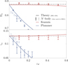 |
Fig. G.1. Pattern speed (top) and growth rate (bottom) of the dominant mode in Zang ν = 4 disc (Zang 1976), as a function of the rescaled softening length, εF (Equation G.5), for the Plummer softening kernel (blue – Equation G.2) and the Kuzmin kernel (red – Equation G.3). The theoretical predictions (plain lines) are reproduced from DR+19b (Figure 3 therein), with the dashed line corresponding to the Newtonian (non-softened) prediction from Evans & Read (1998) (table D1b therein). The N–body measurements are from Sellwood & Evans (2001) (faint dots SE01 – Plummer softening only – Figure 1 panel b therein), and our own measurements (plain dots – both kernels). Here, we recover that the Plummer kernel has a strong gravity bias, i.e. a predicted change in the mode’s property |
In this appendix, we conduct a similar investigation for the Zang ν = 4 disc (same as Sellwood & Evans 2001), using both the Plummer and Kuzmin kernels. The results are presented in Figure G.1. On the N–body front, for each kernel and softening length, we performed 10 independent realisations with N = 2 × 10⁸ particles each. We found that the unstable modes were indeed less affected by the Kuzmin kernel compared to the Plummer kernel. Our numerical measurements align with the predictions from DR+19b as well as the earlier results of Sellwood & Evans (2001). However, it is important to note that in this figure, the N–body errors are likely underestimated: Sellwood & Evans (2001) did not account for the scatter among different realisations, while we did not include any uncertainties in the mode fits.
In Figure G.1, the softening length, ε, is rescaled. Since Equation (G.1) is invariant under the transformation (Section 2.3 of DR+19b)
 (G.4)
(G.4)
one ought to be careful when comparing softening lengths. Here, we follow DR+19b, and compare the kernels using
 (G.5)
(G.5)
with f′max the maximum value of the derivative of the softening (dimensionless) kernel. Setting εF/ε = 1 for the Plummer softening, one has εF/ε ≈ 2.568 for the Kuzmin softening (table 1 in DR+19b).
All Tables
All Figures
|
Fig. 1. Time evolution of the bisymmetric fluctuations (Equation B.6) in 12 different N–body realisations of the Mestel disc, with N = 25 × 106 particles each, using a running average over 30 dynamical times. The disc is initially stable and slowly relaxes towards an unstable state. Once unstable, the evolution is dominated by an exponentially growing mode before it saturates. The disc’s configuration is illustrated in Figure 2. Interestingly, the dispersion among realisations greatly increases close to the instability. The dashed line at t/tdyn = 150 is the time at which the changes in the DF are measured in Figure 3. |
| In the text | |
|
Fig. 2. Illustration of the typical evolution of a Mestel disc in one N–body simulation, via the surface density (up to R = 8R0) at two different times. During the collisional phase (left), the disc remains reasonably axisymmetric, displaying recurrent weak transient spirals. After the phase transition (right), the disc develops strong bisymmetric fluctuations, which ultimately saturate (Figure 1), up to the late formation of a bar (see Figure 10 in F+15). |
| In the text | |
|
Fig. 3. Top: Local relaxation rate, ∂F/∂t, in action space as predicted by BL (Equation 3) for the Mestel disc (Section 2.1), computed in the centre of the action bins. The red regions correspond to an increase in the number of particles, while the blue contours correspond to a depletion. Bottom: Relaxation rate measured in N–body simulations of the same disc, averaged over 1 000 realisations with N = 25 × 106 particles each. The changes in the DF are computed at t/tdyn = 150, safely before the discs become unstable (Figure 1). The prediction and measurement are in good agreement, both in shape and amplitude. Slices in action space are illustrated in Figure 4. Collective effects play a crucial role in shaping the long-term evolution of razor-thin discs. |
| In the text | |
|
Fig. 4. Slices of the local relaxation rate, ∂F/∂t, from Figure 3 for fixed Jr (top) or fixed L (bottom), as predicted from BL (dashed) and measured in N–body simulations (full lines). Here, ∂F/∂t in the top (resp. bottom) panel has been averaged over an interval of width δJr = ± 0.02 (resp. δL = 0.06) and subsequently smoothed with a running average of width δL = 0.03 (resp. δJr = 0.01). For the N–body, we measured ∂F/∂t in each realisation independently, estimated the standard deviation among the sample of realisations, and represented the level lines one standard deviation away from the mean value. |
| In the text | |
|
Fig. 5. Relaxation rate, ∂F/∂t, as predicted by the Landau equation (see Appendix F), using the same convention as in Figure 3. The Landau equation predicts a more isotropic diffusion. In addition, the relaxation time predicted by BL is three orders of magnitude shorter than that predicted by Landau: the collective amplification is instrumental. |
| In the text | |
|
Fig. 6. Illustration of the connexion between a disc’s long-term relaxation and the disc’s linear damped modes. In each panel, we represent in the top plot the relaxation rate in action space, predicted by BL, using the same convention as in Figure 3. In the bottom plot, we represent the disc’s susceptibility, |N(ω)| (Equation C.6) represented at the circular angular momentum corresponding to their ILR (see Equation 4). The numerical saturation of the susceptibility for damped frequencies, γ < 0, is to be expected (see e.g. Appendix B in Petersen et al. 2024). Top: Prediction purposely using an insufficient number of basis elements (Appendix C.1) and too few resonances, for illustration purposes. In that case, the disc’s susceptibility contains three clear damped modes. These modes have a direct signature in the BL relaxation rate. The black line corresponds to the ILR resonance line associated with each mode, while the dashed lines correspond to the direction of diffusion. The proximity of these two lines enhances the efficiency of ILR for heating the disc. Bottom: Same as above, but using a numerically converged linear susceptibility, namely using the same parameters as in Figure 3. In both figures we show that the disc’s long-term heating is strongly enhanced at resonance with the underlying weakly damped modes. |
| In the text | |
|
Fig. 7. Figure from S12. Power spectra of the ℓ = 2 fluctuations as a function of radius in their N–body simulation. The presence of three peaks in these early power spectra, and their location at their respective ILR, is likely the resonant signature of weakly damped modes. |
| In the text | |
|
Fig. 8. Same as Figure 1, but for various softening lengths, ε, and two different softening kernels (Appendix G). The level of transparency corresponds to different softening lengths (Equation G.1) with the bottom (resp. top) line corresponding to 20% (resp. 80%) contours over 100 independent realisations with N = 25 × 106 particles. The case Kuzmin ε = 0.16 corresponds to Figure 1. For the Plummer kernel, the larger the softening length, the slower the relaxation, and the more delayed the transition to instability. This kernel introduces a strong gravitational bias when compared with non-softened theoretical predictions (Figure G.1). On the contrary, simulations using the Kuzmin kernel behave similarly across softening lengths. Interestingly, we note that, in every case, the dispersion among realisations increases near phase transition. |
| In the text | |
|
Fig. 9. Relaxation rate, ∂F/∂t, measured in 12 independent N–body realisations, using the same convention as in Figure 3. The number, location, amplitude, and birth time of the action ridges vary strongly from one realisation to another. This is a measure of a long-term stochasticity in the vicinity of the phase transition (see also Figure 4). |
| In the text | |
|
Fig. B.1. Time series of the unwrapped phase (top) and the norm (bottom) of the bisymmetric fluctuations probed by A2(t) from Equation (B.6) over ten independent realisations of the unstable Zang ν = 4 disc (Zang 1976). Each simulation is performed with N = 2 × 10⁸ particles using the Plummer softening kernel (Equation G.2) and for varying softening lengths, ε. For each ε, the same ten initial conditions are used and shown in the same colour. The frequency ΩM (resp. growth rate γM) of the mode are estimated by a linear fit of the phase (resp. log of the norm) of such time series, only using t ≥ Tmin = 10 tdyn. The growth of the phase is generically more regular than the growth of the norm. The Plummer softening kernel introduces a strong gravity bias when compared with (non-softened) theoretical predictions. |
| In the text | |
|
Fig. B.2. Same as in the bottom panel of Figure 3, but presenting here the standard deviation of the local relaxation rate, Nσ(∂F/∂t), over the available realisations. The scatter among different realisations is particularly significant, when compared with the average amplitude from Figure 3. |
| In the text | |
|
Fig. B.3. Same as in the bottom panel of Figure 3. Compared to the fiducial run (top left), we either halved the integration timestep (top right); halved the softening length (bottom left); or doubled the sizes of the Cartesian, radial, and azimuthal grids (bottom right). In all cases, the measurements of the local relaxation rate are fully consistent with one another. Here, the use of the Kuzmin softening kernel (Appendix G) is instrumental to obtain consistent results over a wide range of softening lengths (see Section 4.3). |
| In the text | |
|
Fig. B.4. Same as Figure B.3 but, here, focusing on a single realisation. The structures of the relaxation rate in action space are all consistent with one another. |
| In the text | |
|
Fig. B.5. Same as in the bottom panel of Figure 3, but focusing here on later times, i.e. beyond the disc’s initial slow collisional evolution (Figure 1). The rate of change of the DF is estimated through simple time differences, as indicated in each panel. In each panel, the colours are rescaled to the minimum and maximum value of the local relaxation rate in that panel, as indicated therein. For simplicity, even at late times, actions remain evaluated within the disc’s initial unperturbed axisymmetric potential from Equation (1). |
| In the text | |
|
Fig. B.6. Same as Figure B.5, focusing here on three independent realisations (different columns). The structures of the diffusion in action space differ widely between realisations. Stochasticity is significantly enhanced during the disc’s dynamical phase transition throughinstability. |
| In the text | |
|
Fig. G.1. Pattern speed (top) and growth rate (bottom) of the dominant mode in Zang ν = 4 disc (Zang 1976), as a function of the rescaled softening length, εF (Equation G.5), for the Plummer softening kernel (blue – Equation G.2) and the Kuzmin kernel (red – Equation G.3). The theoretical predictions (plain lines) are reproduced from DR+19b (Figure 3 therein), with the dashed line corresponding to the Newtonian (non-softened) prediction from Evans & Read (1998) (table D1b therein). The N–body measurements are from Sellwood & Evans (2001) (faint dots SE01 – Plummer softening only – Figure 1 panel b therein), and our own measurements (plain dots – both kernels). Here, we recover that the Plummer kernel has a strong gravity bias, i.e. a predicted change in the mode’s property |
| In the text | |
Current usage metrics show cumulative count of Article Views (full-text article views including HTML views, PDF and ePub downloads, according to the available data) and Abstracts Views on Vision4Press platform.
Data correspond to usage on the plateform after 2015. The current usage metrics is available 48-96 hours after online publication and is updated daily on week days.
Initial download of the metrics may take a while.