| Issue |
A&A
Volume 699, July 2025
|
|
|---|---|---|
| Article Number | A24 | |
| Number of page(s) | 28 | |
| Section | The Sun and the Heliosphere | |
| DOI | https://doi.org/10.1051/0004-6361/202553775 | |
| Published online | 27 June 2025 | |
A statistical study of energetic particle events associated with interplanetary shocks observed by Solar Orbiter in solar cycle 25
1
Institute of Experimental and Applied Physics, Kiel University, Kiel, Germany
2
European Space Agency (ESA), European Space Astronomy Centre (ESAC), Camino Bajo del Castillo s/n, 28692 Villanueva de la Cañada, Madrid, Spain
3
Universidad de Alcalá, Space Research Group (SRG-UAH), Plaza de San Diego s/n, 28801 Alcalá de Henares, Madrid, Spain
4
The Blackett Laboratory, Department of Physics, Imperial College London, London SW7 2AZ, UK
5
Department of Physics and Astronomy, University of Turku, Turku, Finland
6
Institute for Theoretical Physics and Astrophysics, University of Würzburg, Würzburg, Germany
7
Department of Physics, University of Helsinki, P.O. Box 64 FI-00014 Helsinki, Finland
8
Heliophysics Science Division, NASA Goddard Space Flight Center, Greenbelt, MD 20771, USA
⋆ Corresponding author: This email address is being protected from spambots. You need JavaScript enabled to view it.
Received:
15
January
2025
Accepted:
25
March
2025
Abstract
Context. We studied energetic particle intensity profiles observed by Solar Orbiter during the time period from April 2020 to April 2023, associated with the passage of interplanetary (IP) shocks. For our study we considered 58 IP forward shocks and analysed the possible correlations between some IP shock parameters and the electron and proton responses to the passage of the IP shocks. We investigated which shock signatures are more likely related to the efficiency of the IP shocks with respect to particle acceleration.
Aims. We introduced a variable that characterises the contamination induced by protons in the electron channels of the Electron Proton Telescope (EPT) part of the Energetic Particle Detector (EPD) suite of instruments on board Solar Orbiter, which allowed us to identify the cases in which the intensity time profiles of electrons at energies ≤240 keV showed a real response at the passage of IP shocks. In the case of protons, we searched for the response in seven energy ranges from 52 keV to 15 MeV, and based on the shape of the proton response at low energies (∼100 keV), we divided the profiles into weak responses, peaks (regular or irregular), plateaus, and unclear responses. For the regular peak and plateau types we constructed an average time profile by applying superposed epoch analysis. For the response in electrons and protons, and for the different types of proton responses at different energies, we analysed the corresponding IP shock parameters, aiming to understand which ones are important to form a certain type of time profile or to achieve a certain energy. We also included a comparison between the proton intensity time profiles in the upstream region and, assuming the predictions of the diffusive shock acceleration (DSA) theory, identified the values of the mean free path in several cases.
Methods. We found that the IP shock efficiency in the energisation of both electrons and protons is strongly energy dependent. Cases of electron acceleration are rare. Only in about ∼8% of the events for energies ≤100 keV and in ∼2% for energies ≤250 keV did the electron intensities show an unambiguous response at the passage of IP shocks (with those accompanied by a response being mainly oblique or quasi-perpendicular). The shocks for which we identified a response in ∼100 keV proton intensity time profiles come to ∼83% of the IP shocks under study, and are parallel or quasi-parallel. The ability to accelerate protons to higher energies and to form a particular shape of the particle response to the IP shock passage mostly depends on the IP shock speed.
Results. Based on the analysis of time profiles and the occurrence of unambiguous electron acceleration at shocks, the acceleration mechanism behind the electron energisation is unlikely to be DSA, but shock drift acceleration (SDA) remains a candidate for the acceleration mechanism. Proton time profiles of the plateau type around the IP shock front can be achieved with an IP shock speed above 800 km s−1 and an ambient mean free path ≤0.015 au, reproducing the asymptotic steady-state ion distribution reached in the classical DSA solution.
Key words: Sun: heliosphere / Sun: particle emission
© The Authors 2025
 Open Access article, published by EDP Sciences, under the terms of the Creative Commons Attribution License (https://creativecommons.org/licenses/by/4.0), which permits unrestricted use, distribution, and reproduction in any medium, provided the original work is properly cited.
This article is published in open access under the Subscribe to Open model. This email address is being protected from spambots. You need JavaScript enabled to view it. to support open access publication.
1. Introduction
Energetic storm particle (ESP) events in which energetic particle increases are associated with the passage of an IP shock were identified by Bryant et al. (1962, 1965). Currently IP shocks are considered to be efficient particle accelerators, as theoretically justified by the theories of Krymskii (1977) and Drury (1983), which relate the spectrum of the accelerated particles to the gas compression ratio at the shock, and also the spatial dependence of the particle time profiles in the upstream and downstream regions (e.g. Drury 1983). While the ability of IP shocks to accelerate ions is not questioned, the parameters that are most relevant for accelerating them to higher energies are still elusive, as are the possible role of IP shocks in accelerating electrons.
Several studies investigated electron flux enhancements in the vicinity of IP shocks. For example, Dresing et al. (2016) analysed 475 IP shocks observed by the Solar-TErrestrial RElations Observatory (STEREO) (Kaiser et al. 2008) within the time period from 2007 to 2013. For ∼70 keV electrons, intensity enhancements were found in only 1% of the analysed cases. Electron flux increases were observed only in five IP shock passages in which the shock angles were ΘBn = 31° in one event, and ΘBn ≥ 75° for the remaining four events.
In a number of studies, the role of IP shocks and the associated plasma parameters favourable for shock acceleration were investigated. Kallenrode (1996) studied data obtained from the Helios mission, spanning the time period from February 1976 to March 1980, and investigated a possible dependence of the positions of the spacecraft with respect to the IP shock nose. Neglecting local perturbations, the nose of the shock is understood as the most distant region of the shock with respect to the Sun. Kallenrode (1996) found that the acceleration was most efficient in the nose region of IP shocks. Rodríguez-Pacheco et al. (1998) studied the connection between the characteristics of particle (mainly proton) fluxes and IP shocks during solar cycle 21. They found a clear correlation between the observed particle spectral indices and the IP shock compression ratios, and furthermore that the most powerful particle increases were observed at locations of small separation angles between the associated flare and the spacecraft magnetic foot point, suggesting that the acceleration takes place close to the IP shock nose. In addition, the lower energy particles (E ≤ 50 keV) seemed to be more responsive to the variation of shock parameters than the higher energy particles. A study by Lario et al. (2005) of forward IP shocks observed by the Advanced Composition Explorer (ACE) spacecraft (Stone et al. 1998) from 1998 to 2003 showed a tendency for faster and stronger (higher compression ratios) IP shocks to be associated with higher particle intensities (47–68 keV proton) related to the IP shock passage. Dresing et al. (2016) also observed increases of ∼100 keV and ∼1 MeV ions in 27% and 5%, respectively, of the IP shocks observed with the STEREO spacecraft.
The present work investigates the relations between both widely and not so commonly used shock parameters, and the associated in situ time profiles of energetic particles (electrons and protons). The main goal of the study is to identify the IP shock parameters that determine the responses in the electron and proton fluxes associated with the passage of an IP shock. To achieve this goal, we used the in situ list of IP shocks observed by the Solar Orbiter mission (Müller et al. 2020) from April 2020 to April 2023, compiled by Trotta et al. (2023b, 2025), and the electron and proton fluxes measured by the EPT and the High Energy Telescope (HET) as part of the EPD suite (Rodríguez-Pacheco et al. 2020; Wimmer-Schweingruber et al. 2021) on board Solar Orbiter. In particular, we investigated which IP shock parameters indicate an efficient acceleration of ions up to higher energies (≥5 MeV/n), and form different types of proton intensity time profiles. For this purpose, we performed a statistical analysis of the IP shock parameters and compared them with the particle profiles associated with the passage of the IP shocks. A data analysis is presented in Sect. 2. The analysis of the electron response to the passage of IP shocks is shown in Sect. 2.1, including a case analysis for all electron events found in the study. Section 2.2 presents a comprehensive analysis of the different types of proton responses to the passage of IP shocks and their dependence on proton energies. A comparison of the observed proton intensity time profiles with predictions of DSA theory is presented in Section 2.3. Section 3 presents the summary and discussion. Finally, Section 4 summarises the main conclusions of the study.
2. Data analysis
We used a list of IP shocks observed between April 2020 and April 2023, compiled by Trotta et al. (2023b) and prepared within the Solar Energetic Particle Analysis Platform for the inner heliosphere (SERPENTINE)1 project. Later Trotta et al. (2025) added the shocks observed from May to December 2023, bringing the total list to 101 shocks. That paper presented a detailed analysis of shock parameters as a function of radial distance and intercorrelations between the shock parameters, but it did not offer an in-depth study of how these parameters affect electron and proton acceleration. For shock identification, the Tracking and Recognition of Universally Formed Large-scale Shocks (TRUFLS) code (Trotta et al. 2025) was applied, which uses a moving average to monitor the magnetic field magnitude, the solar wind plasma density, and the solar wind speed for a relevant period of time, identifying the instants of time in which these quantities present discontinuities (jumps). Following this procedure, 61 IP shocks2 were identified by Trotta et al. (2023b, 2025), three of them being reverse shocks (see Trotta et al. 2024c). For each event analysed an extensive characterisation of the shock and ambient key parameters was carried out. It is worth noting that the shock parameter estimation is subject to non-negligible uncertainties, especially for single-spacecraft crossings (e.g. Koval & Szabo 2008). Such uncertainties arise both from the intrinsic nature of the shock parameters estimation relying on strong assumptions, such as the validity of the Rankine-Hugoniot jump conditions, and from the upstream or downstream averaging process of the magnetic field and plasma quantities (Paschmann & Schwartz 2000). To mitigate the limitations arising from the choice of upstream or downstream averages, key ambient and shock parameters were estimated using the SerPyShock method (Trotta et al. 2022). This method uses a systematic variation of time averaging windows involved in the single-spacecraft diagnostics for the shock parameter estimation (Paschmann & Schwartz 2000), which in this study was chosen to be between one and eight minutes. Such systematic variations of averaging windows enables the examination of a distribution of shock parameters for each choice, allowing for the assessment of uncertainties associated with the parameter estimation. We find that these uncertainties can be as large as 20% for parameters such as the shock normal angle or the shock speed, in particular for events characterised by strong structuring of the local plasma.
The key IP shock and ambient plasma parameters used in this study are listed in Column 1 of Table 1, also including the radial positions of the spacecraft at the moment of the IP shock identification. The level of upstream magnetic field fluctuations δB/B0 was computed combining the component as δB/B0 ≡ |B(t + τ)−B(t)|/|B(t)|, where the lag τ was chosen as one minute, and then averaged for eight minutes in the upstream or downstream region of the IP shock. The mean values of the upstream solar wind density and the plasma β were averaged for eight minutes upstream of the IP shock. Some of the above parameters had been explored in previous studies in connection with energetic particle enhancements, as discussed in Sect. 1. However, to our knowledge the use of the parameters related to the fluctuations of solar wind plasma and magnetic field represents a novel approach in statistical studies.
Shock parameters (Trotta et al. 2024a) with and without electron and proton response.
We note that some of the aforementioned parameters can be only defined if both plasma and magnetic field data are available and therefore, several IP shocks do not have all parameters listed. To investigate the proton response we used only those IP shocks for which the shock speed, gas compression ratio, Alfvénic Mach number, upstream solar wind density, and upstream plasma β were available. As the response of energetic electrons to the IP shock passage is usually more rare than that of protons, and in order to have a better estimate of the fraction of cases with electron response, we kept those IP shocks in the electron study for which only a few parameters were known. We also excluded from the statistics the shocks on 18 July 2021, 19 July 2021 and 16 February 2022. The period of the shock passage within plus and minus one day was characterised by elevated electron fluxes in all of the cases mentioned above. Nevertheless, at the moment of the shock passage, there was no obvious increase coinciding with the shock passage, and the discussion about the origin of the electrons preceding the shocks is out of the scope of the present paper. The shock on 6 September 2022 was excluded as well from the calculation of the average values because of a disagreement between HET and Suprathermal Ion Spectrograph (SIS) data during this event, and a possibility of an additional instrumental effect.
We included in our statistical study only forward IP shocks, and taking into account also the gaps in particle data and special cases to consider electrons, our final reduced list to study electron (proton) responses includes 51 (48) IP shocks. In Table 1 we present the average, median, and standard errors of the 51 IP shock parameters as a sample for comparison in part of the electron study (Col. 2), and of 48 shocks involved in the part related to the proton study (Col. 3). As not all parameters were available for all IP shocks, we also indicate in Table 1 the number of shocks used to obtain the corresponding values. Table A.1 shows how the averaged parameters change if we consider all forward IP shocks from the list by Trotta et al. (2023b, 2025) (Col. 2), or only those IP shocks (44) where all the listed parameters are available (Col. 3).
To investigate the energetic particle response for each of the IP shocks identified in the study, we analysed the time profiles of electrons and protons measured in situ by Solar Orbiter around the time of the IP shock. Our analysis is based on the particle fluxes measured by the HET instrument (only used for protons) and by the foil and magnet telescopes of EPT, respectively measuring electron and ion intensities (Rodríguez-Pacheco et al. 2020).
The EPT instrument utilises the Magnet-Foil technique to separate electrons and ions from each other. While the magnet detectors measure the ion flux only, the foil detectors are designed to measure electrons with the foil stopping ions of similar energies. However, Wraase et al. (2018) show that the impact of ion fluxes on electron measurements can be large, especially in periods with enhanced ≥450 keV proton intensities, as expected during the passage of IP shocks. Moreover, it is known that the foil detector on EPT measures protons and helium ions in the electron channels starting above 34 keV, which can be crucial to separate the signal coming from electrons around IP shock passages when the ion fluxes are especially high. Therefore, a critical problem of any study involving electron intensity time profiles in the vicinity of an IP shock passage is to separate the signal produced by protons and ions in the foil detectors from the signal coming from electrons.
Taking into account the difficulties of assessing the signal in electron channels around an IP shock passage as being created by electrons, our analysis included several steps. First, we used the corrected electron level 3 data provided by the SERPENTINE project3, which uses an estimate of the helium-to-proton ratio derived from the EPT measurements on the time scale of 10 minutes, leveraging the distinct responses of the magnet and foil channels to helium. Nevertheless, during periods of rapidly fluctuating ion fluxes, such as those encountered during IP shocks, this estimation could be less reliable and potentially introduce systematic errors into the corrected electron intensities. Taking into account that electrons at ≥50 keV are faster than protons in the energy range of 200–700 keV, and also have a larger mean free path resulting in larger spatial diffusion coefficients, their intensity time profiles should look different. To reject the cases around the IP shocks where protons and ions could still have a dominant effect, we have introduced the contamination parameter
 (1)
(1)
where Icorrected and Iuncorrected represent corrected and uncorrected electron intensities, respectively. We then assume that the corrected electron intensities represent real electron fluxes if the contamination parameter is below ∼0.6. This limit is introduced to account for potential systematic errors in the corrected electron fluxes. Systematic errors in the correction can result from rapidly fluctuating ion fluxes and errors in the simulated instrument response functions that are used in the correction. These errors can lead to an underestimation of the contamination, and thus to an overestimation of the corrected electron flux. As a result, even in the absence of actual electrons, the contamination parameter does not necessarily reach values of 1. By evaluating apparent upper limits of the contamination parameter during various strongly contaminated periods and by considering possible systematic errors, we estimate an approximate limit of 0.6 for this parameter. Above this limit, we assume that systematic errors prevent a reliable estimation of the contamination.
Furthermore, we consider a possible contamination from > 20 MeV protons which, in addition to the previous estimate, could contaminate the EPT electron detectors. To estimate that contamination, proton count rates in the EPT electron detectors are calculated from HET proton flux measurements up to 100 MeV, using proton response functions obtained from Geant4-based simulations. The residuals between the measured count rates and the calculated proton count rates are attributed to electrons. If an event had no clear residuals we considered it to be contaminated by high-energy protons and do not consider it as having a response in electrons.
Finally, we made an additional verification for the presence of an electron response to the IP shock passage by comparing the spectrogram plots for electron and proton data, along with solar wind parameters and magnetic field measurements around the IP shock passage, and rejected the cases where peaks around the shock passage by chance coincided with solar sources (flares) or were connected with geomagnetic activity when Solar Orbiter was making a gravity assist manoeuvre at Earth.
Because of the large number of figures in this paper, we have moved several figures to appendices, but will occasionally refer to them. Figures B.1 and B.2 show two shocks where high-energy protons were responsible for a peak around the passing shock. Figure C.1 shows a spectrogram from the EPT magnet (left) and foil (right) observations along with solar wind parameter and magnetic field data around the IP shock on 27 November 2021, which was rejected from the study. Solar Orbiter was located close to Earth after the gravity assist manoeuvre and it could have been well magnetically connected to the magnetosphere or to the bow shock.
Additionally, in Appendix F we show a spectrogram plot for the remaining IP shock on 8 June 2022, which was assessed as a plateau type of response for protons discussed in Sect. 2.2 and characterised by strong contamination by protons in EPT, which we cannot assess as a response in electrons to the IP shock passage.
2.1. Electron response to IP shocks
We analysed energetic electron time profiles obtained by the EPT instrument for the periods around the listed IP forward shock passages. We used three energy channels within the near-relativistic range: 35.6–63.5 keV, 63.5–121 keV, and 121–238 keV. In this investigation we are interested in the local acceleration of electrons around the shock, for which we could accurately determine the observed local parameters. We define the term “electron response” as an increase of the omni-directional electron intensity in connection with the IP shock passage, by at least two times over the pre-shock background level, taken several hours before the shock. This intensity increase should coincide with the passage of the shock front, or occur shortly after the shock (typically a few minutes). As discussed above, we checked the contamination variable defined in Eq. (1), examined the corresponding spectrogram plots and took into account the contamination due to high-energy protons and the directional data, and found that the energetic electrons showed responses related to four of 51 (8%) IP shocks. Such an electron increase was observed for the following IP shock passages: 22 August 2021 at 7:46 UT, 3 November 2021 at 14:04 UT, 21 May 2022 at 14:51 UT, and 25 July 2022 at 6:22 UT. Only in one case out of 51 (2.0%) we observed acceleration to energies ≥100 (up to 250) keV associated with the IP shock passage. In this case, on 25 July 2022, the IP shock angle was ΘBn = 61°.
Figures 1 and 7, respectively, show from top to bottom the time profile of protons, electrons (solid lines indicate uncorrected data, dotted lines corrected data), and the parameter Ccont described in Eq. (1) for the two cases (22 August 2021 and 21 May 2022) where an electron increase after the shock passage is clearly visible only in the omni-directional data. Both figures are centred at the time of the shock front passage, and cover 12 hours before and after the shock.
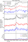 |
Fig. 1. Particle response to the IP shock on 22 August 2021 with ΘBn = 88°. From top to bottom the panels show the time profile of protons, electrons (solid line – uncorrected, dotted line – corrected), and Ccont. The insets show the colour-coding used for the different energy channels. The vertical solid line indicates the IP shock arrival. Rsc = 0.65 au. |
Figures 2, 6, 8 and 11, respectively, show the electron (right panel) and proton (left panel) response around the time of the IP shock passage for each of the four events identified above. The top panel shows the solar wind speed (black curve, left axis), temperature (red curve, right axis), and number density (blue curve, right axis). The following four panels show proton (left) and uncorrected electron (right) spectrograms for the four detectors, with the intensity indicated by the colour bar shown on the right, and the energy given on the left axis for each panel. The dashed curve over each spectrogram shows the pitch angle (right axis) for each detector. The lowest panel shows the absolute value of the magnetic field (black curve, left axis), polar (blue curve, right axis), and azimuthal (red curve, right axis) angles. All figures are centred at the time of the IP shock passage (vertical dashed line) covering the period of one hour before and after the IP shock arrival. We discuss in detail each of these electron events below.
 |
Fig. 2. Particle response to the IP shock on 22 August 2021. Top panel: Solar wind speed (black curve, left axis), solar wind temperature (red curve, right axis, kT), solar wind number density (blue curve, right axis). Middle four panels: EPT foil (left) and magnet (right) observations by Solar Orbiter from different telescopes, as indicated in the upper right corner of each panel. The pitch angle is shown as a dot-dashed line (right axis). The colour bar on the right shows the intensity. Bottom panel: Magnetic field magnitude ∣B∣ (black curve, left axis), and polar (red curve, right axis) and azimuthal (blue curve, right axis) angles. The vertical dashed line indicates the IP shock arrival. |
2.1.1. Electron response to the IP shock on 22 August 2021
The response of electrons and protons to the IP shock passage on 22 August 2021 is shown in Figures 1 and 2, respectively. The IP shock exhibited Mach numbers of 7.4 (Alfvénic) and 4.4 (fast magnetosonic), respectively, a speed of 437 km s−1, and values of 1.5 and 1.1 for the magnetic and gas compression ratios, respectively. The value of the shock normal angle was ΘBn = 88°, which corresponds to a perpendicular IP shock. We note, however, that the compression ratios are abnormally small for a high Mach number perpendicular shock, which might be a local effect due to the inhomogeneous upstream plasma.
The region upstream of the shock shows a spike in proton and electron energy channels about an hour before the shock arrival. Otherwise, there does not seem to be any foreshock region, which is understandable given the near-perpendicular geometry. The flux increase trails the shock and could be caused by SDA under weak scattering conditions (e.g. Lario et al. 2005). However, DSA would have to rely on perpendicular diffusion in this geometry, which is probably not a very likely scenario.
2.1.2. Particle response around the 3 November 2021 IP shock
The constellation of the spacecraft for this event is shown in Figure 3 (Gieseler et al. 2023). The IP shock exhibited Mach numbers of 3.2 (Alfvénic) and 2.9 (fast magnetosonic), a speed of 502 km s−1, and values of 1.9 and 2.2 for the magnetic and gas compression ratios, respectively. However, the shock parameter analysis involving very short (local) averaging indicates that it might have been stronger locally (Trotta et al. 2023a; Yang et al. 2023). The value of the shock normal angle is ΘBn = 42°, which would correspond to an oblique IP shock. The time profiles of electrons (corrected data) and high-energy protons to the IP shock passage on 3 November 2021 at 14:04 UT are shown in Fig. 4 and demonstrate a striking similarity. To verify whether the signal in the electron detector was due to real electrons we made an estimate of the contribution of the high-energy protons to the signal measured in the electron channel. Figure 5 shows a comparison of the measured count rate in the EPT electron detector with the calculated count rate from protons up to 100 MeV in the same detector. Residuals indicate that electrons up to about 100 keV (energy channel 17) were observed. A spectrogram for this event is given in Fig. 6. The right panels of the figure show a clear jump in the electron flux at 14:15 UT when the spacecraft possibly entered a region with an opposite field direction, or a pair of rotational discontinuities – a so-called switchback – which caused a stronger jump in the azimuthal angle ϕ (lowest panel) and changes of the pitch angles for the sun (second panel) and anti-sun detectors (third panel). In total, three IP shocks were detected by Solar Orbiter on 3 November 2021. The first IP shock observed at ∼08:00 UT was perpendicular, with ΘBn = 89°, and could have produced a seed population. The second IP shock arrived at ∼12:30 UT with a shock normal angle of ΘBn = 41°. The third and last shock was the one associated with the electron response shown in Fig. 6. We note that the second and third shocks were oblique and exhibited similar shock angles, which promoted both the opportunity for particles moving from upstream to downstream to reflect off the shock, and the possibility to drift along the shock front and thus to gain energy as a result of the electric field. This situation could have resulted in the higher electron increase after the last (third) IP shock passage, suggesting that such a sequence of IP shocks can be an efficient particle accelerator (e.g. Niemela et al. 2024).
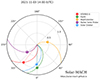 |
Fig. 3. Constellation of spacecraft at the time of the shock passing Solar Orbiter at 14:04 UT. |
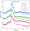 |
Fig. 4. Proton time profiles and corrected electron time profiles associated with the IP shock passage on 3 November 2021 at 14:04 UT. The energy ranges are given in the legend. Rsc = 0.42 au. |
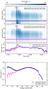 |
Fig. 5. Particle response to the IP shock on 3 November 2021 at 14:04 UT. From top to bottom: Measured count rate in foil Sun detector, calculated count rate in foil Sun detector, count rate in energy channels 10–14 as a function of time, count rate spectrum for the period of time indicated as “tp1” in the top two panels. |
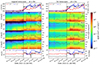 |
Fig. 6. Particle response to the IP shock on 3 November 2021. Legend and panel description as in Fig. 2. |
2.1.3. Electron response to the IP shock on 21 May 2022
The response of electrons and protons to the IP shock passage on 21 May 2022 is shown in Figs. 7 and 8. The IP shock exhibited Mach numbers of 5.3 (Alfvénic) and 4.2 (fast magnetosonic), a speed of 420 km s−1, and values of 2.0 and 1.9 for the magnetic and gas compression ratios, respectively. The value of the shock normal angle was ΘBn = 80°, which would correspond to a quasi-perpendicular shock.
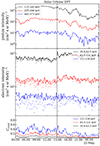 |
Fig. 7. Electron response to the IP shock on 21 May 2022 with ΘBn = 80°. Description and legend as in Fig. 1. |
The electron fluxes increase quite abruptly at the shock, and there is no electron foreshock observed in this IP shock passage. This is consistent with the SDA mechanism being the dominant one, similar to the case on 22 August 2021.
2.1.4. Electron response to the IP shock on 25 July 2022
As on 3 November 2021, high-energy protons were observed around the shock on 25 July 2022. The time profiles of corrected electron and proton intensities in connection with the IP shock passage on 25 July 2022 are shown in Fig. 9. The IP shock was more powerful than the events discussed previously, as it exhibited Mach numbers of 8.4 (Alfvénic) and 7.0 (fast magnetosonic), a speed of 820 km s−1, and values of 2.9 and 2.5 for the magnetic and gas compression ratios, respectively. The value of the shock normal angle was ΘBn = 61°, which would correspond to a quasi-perpendicular IP shock (Trotta et al. 2025).
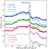 |
Fig. 9. Proton time profiles (lines) and corrected electron time profiles (dots) associated with the IP shock passage on 25 July 2022. The energy ranges are given in the legend. |
Figure 10 shows a comparison of the measured count rates, and the calculated count rates in the electron channels due to protons. Residuals indicate that electrons up to about 250 keV (energy channel 27) were observed. The spectrogram plot for this event is shown on Fig. 11. Prior to the shock, especially in the south telescope (fifth panel in Fig. 11) we can clearly see a precursor, which fits the prediction of Decker (1983) for SDA of particles energetic enough so that they can escape upstream from the shock. This does not preclude other acceleration mechanisms operating at the shock transition layer to account for the event, such as stochastic SDA, which has been shown to agree with observations at the Earth’s bow-shock (Amano et al. 2020, 2024). After the IP shock, the spacecraft travelled through several magnetic flux tubes (at ∼06:31 and 06:35 UT) with different density of electrons which dropped suddenly when the spacecraft went to the flux tube characterised by higher temperature (first panel in Fig. 11). This unusual configuration of the IP magnetic field, when before the shock arrival and shortly afterwards the magnetic field was oriented along the south-north direction (lowest panel in Fig. 11), is favourable for SDA to take place at the IP shock front, assuming that the shock normal direction is close to radial. The electron response to the shock was also analysed by Jebaraj et al. (2023).
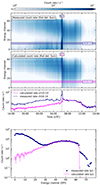 |
Fig. 10. Particle response to the IP shock on 25 July 2022. From top to bottom: Measured count rate in the foil Sun detector, calculated count rate in foil Sun detector, count rate in energy channels 10–14 as a function of time, count rate spectrum for the period of time indicated as “tp1” in the top two panels. |
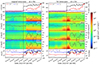 |
Fig. 11. Particle response to the IP shock on 25 July 2022. Legend and panel description as in Fig. 2. |
2.1.5. Averaged parameters of IP shocks with response in electrons
The averaged values of the IP shock and plasma parameters for the IP shocks with response in electrons, together with the radial locations of the spacecraft at the moment of the shock passage are given in Column 4 of Table 1. We compared these parameters with the average values given in Column 2 for the reduced list of 51 IP shocks, for which we searched for electron enhancements in connection with shock passages. The IP shocks which exhibited an electron response show a larger angle between the shock normal and the magnetic field, being more oblique and/or perpendicular, namely ⟨ΘBn⟩ = 68° ±9° compared to ⟨ΘBn⟩ = 54° ±3° for the initial sample. They exhibit higher average Alfvénic Mach numbers, namely 6.1 ± 1.0 compared to 3.3 ± 0.3, higher average fast magnetosonic Mach numbers, namely 4.6 ± 0.7 compared to 2.8 ± 0.3 and lower average level of upstream magnetic field fluctuations, namely 0.17 ± 0.04 compared to 0.25 ± 0.02. If one takes into account that the ratio of downstream to upstream fluctuations is the same for shocks with response in electrons and the sample, one can conclude that the turbulence level around the shock front in both upstream and downstream regions is lower. While the values of the solar wind number density and plasma beta in the upstream region are slightly higher, they overlap with the original sample within the value of the standard error. The averaged values of the remaining parameters are also similar.
Therefore, such a difference in the value of the shock angle (⟨ΘBn⟩) is consistent with SDA for electrons, which could be boosted by stochastic processes at the shock (Amano et al. 2020, 2024; Katou & Amano 2019), such as stochastic SDA, when the transition shock region is characterised by extremely strong scattering, allowing for electrons to be subject to SDA in the shock transition region over an extended time. Alternatively, this could be due to multiple SDA cycles, stimulated by a high scattering rate in the downstream region, allowing electrons to return more easily to the upstream region where they can be guided by the inhomogeneous magnetic fields (e.g. Sandroos & Vainio 2006) to enter another SDA cycle. Overall, both processes allow for electrons to experience the process of SDA for a longer time and lead to achieve higher energies.
To draw more definite conclusions regarding the processes lying behind the acceleration of electrons by shocks better statistics would be required. Nevertheless, when the main problem is to distinguish between the signal induced by protons in the electron channel and real electrons one cannot expect to solve this problem, and advanced detectors which do not suffer from the above contamination effects would be needed.
2.2. Proton response to IP shocks
For our analysis we used seven proton energy channels measured by EPT and HET (in parenthesis we show the energy label used in the following figures): 52–60.2 keV (60 keV), 64.5–71.8 keV (70 keV), 91.3–151.4 keV (130 keV), 412–677 (500 keV), 677–1130 keV (1 MeV), 5300-6100 keV (6 MeV), and 14600–15600 keV (15 MeV). We summarise in Column 5 of Table 1 the average values of shock and plasma parameters for the 40 out of 48 (82%) IP shocks which are associated with a proton response at least around 100 keV. This response is energy dependent, however, we note that the novel capabilities of EPD in resolving the dynamics of supra-thermal particles show a rich scenario of proton acceleration at lower energies (Trotta et al. 2023c).
One can define the probability of proton acceleration by IP shocks as the fraction of shocks in which protons above a certain energy have shown a response to the IP shock passage with respect to the number of all shocks considered. We show this probability as a function of proton energy in Fig. 12. The horizontal and vertical error bars represent the energy intervals and the standard error, respectively; moreover the number of shocks used to calculate this fraction for each given energy interval also includes all higher energy intervals. For the two highest energy points the horizontal error bars that correspond to the energy intervals used are smaller than the symbols (circles). The first-order polynomial fitting of the points results in the acceleration probability function,
 (2)
(2)
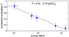 |
Fig. 12. Probability of acceleration as a function of proton energy. The energy intervals are indicated by the horizontal error bars, and the standard error by the vertical error bars. E0 = 1 MeV. Details are given in the main text. |
where E0 = 1 MeV. Equation 2 shows that the probability decreases with increasing proton energy. However, taking into account that in some strong IP shocks (high Mach numbers, high compression ratios) the response in protons is also visible at energies higher than in the present study, we suggest that this distribution presents a tail in the high-energy region (≳15 MeV).
From our study we find that the acceleration probabilities for proton energies ≥100 keV and ≥6 MeV, are 83% (40 out 48) and 17% (8 out of 48), respectively. For comparison, Kallenrode (1996) found a probability of ∼53% for 5 MeV protons. Using STEREO observations at distances close to 1 AU, Dresing et al. (2016) found an acceleration efficiency of 27% for 100 keV ions and 5% for 2 MeV ions. Both of the above values are lower than the ones obtained in the present work. Huttunen-Heikinmaa & Valtonen (2005) found an efficiency of 48% for protons with energies ≥1.5 MeV. Lario et al. (2003), who analysed ACE/Electron Proton and Alpha-particle Monitor (EPAM) data, found an acceleration efficiency of IP shocks for ions with 0.057 and 3 MeV energies of 61% and 33%, respectively. Tsurutani & Lin (1985) found a value of 27% for 1.5 MeV protons. There is a significant variation in the above probabilities obtained by different authors. This can be partially explained by different definitions of the particle response to shocks and, in part, by variations in the shock strength over different time periods, such as those associated with changes in solar activity levels.
Table 2 shows the averaged, median, and standard error values, the number of shocks used for averaging, of the spacecraft location, the IP shock and plasma parameters around the shock front for different types of proton time profiles (discussed below) and comparing two different proton energies (Col. 6 and 7). The parameters listed in Col. 1 of Table 2 with symbols are described with full names in Col. 1 of Table 1. Columns 6–7 of Table 2 show the averaged parameters associated with proton increases with energies ≤100 keV and ≥6 MeV, respectively. We note that Col. 6 lists the cases where protons show response only at ≤100 keV and not at higher energies. The IP shock speed respectively exhibits the main difference between these two groups, ⟨Vsh⟩ = 432 ± 16 km s−1 in comparison to 821 ± 125 km s−1. Moreover, the IP shocks producing a response in protons ≥6 MeV in comparison with response in ≤100 keV are less oblique, namely ⟨ΘBn⟩ = 49° ±6° in comparison to 62° ±5°; exhibit larger average Mach numbers, namely both Alfvénic ⟨MA⟩ = 4.8 ± 0.8 versus 4.1 ± 0.7 and fast magnetosonic ⟨Mfast⟩ = 4.2 ± 0.7 versus 3.0 ± 0.3; and lower average upstream beta, ⟨βup⟩ = 0.57 ± 0.09 in comparison with 1.26 ± 0.28.
Shock parameters for different types of response and energy.
The shape of ion (or proton) response in connection with the IP shock passage can differ from one case to another. In reality, shocks are neither infinite nor planar, but usually feature complicated small-scale structuring (e.g. shock-lets, jets Trotta et al. 2023a; Hietala et al. 2024; Trotta et al. 2024b; Kilpua et al. 2023) that may considerably affect the energetic particle profiles. Moreover, a high pre-shock background can mask the exponential growth towards the shock front. We identified different types of time profiles depending on the shapes of the proton fluxes around the IP shock ±5 hours. We used the types of profiles defined by Trotta et al. (2023b) adding two additional types to classify the events in accordance with the shape of the observed time profile at lower energies, namely ≤100 keV. We divided the profiles into six types, showing in parenthesis the number of IP shocks associated with each type of proton profile: no response (8), weak response (17), regular peak (12), irregular peak (4), plateau (4), and unclear response (3).
We define an ‘insignificant or weak response’ as a proton intensity increase associated with an IP shock passage in the 50–70 keV energy range by less than one order of magnitude in comparison with the pre-shock level (about 3 hours before the shock passage). We consider a ‘regular peak’ to be the cases where a peak in proton intensity happens shortly before the shock or after it, or coincides with the IP shock passage; the profile itself exhibits a regular growth before this peak and has a decay profile in several proton energy channels after the peak. By ‘plateau’ we refer to a sharp increase of more than one order of magnitude at low energies (≤100 keV) within less than one hour, turning into almost constant level of proton intensity after the IP shock passage for at least five hours. As presented above, we classified three IP shocks as unclear response and four shock passages as irregular peak proton response, where two cases were connected with a sequence of several shocks. However, because it was not possible to disentangle the effect of a single shock in case of a sequence of shocks nor to understand what was the exact effect of an isolated shock, we did not include these two types into the statistical analysis. Nevertheless, in Appendix G we show some examples of these types of responses.
In Cols. 2–5 of Table 2 we show the averaged, median, and standard error values of the IP shock and plasma parameters for the different proton response profiles defined as no response, weak response, regular peak, and plateau. An example of a weak response is shown in Fig. 13, exhibiting a slight increase in 60–70 keV proton energies. Three profiles showing the regular peak type response are presented in Figs. 14–16. Figures 14 and 16 show appearance of the peak before and after the shock passage, respectively, and Fig. 15 shows the proton intensity time profiles in different energy channels for the event on 10 April 2023 used in Sect. 2.3 for comparison with DSA prediction.
 |
Fig. 13. Proton time profiles associated with the IP shock passage (vertical line) on 23 October 2021 representing a weak response. The different energy ranges are indicated by the coloured lines (see legend on the right). |
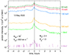 |
Fig. 14. Proton time profiles associated with the IP shock passage on 13 May 2022 representing a regular peak response. Legend and lines as in Fig. 13. |
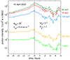 |
Fig. 15. Proton time profiles associated with the IP shock passage on 10 April 2023 representing a regular peak response. Legend and lines as in Fig. 13. |
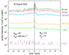 |
Fig. 16. Proton time profiles associated with the IP shock passage on 30 August 2022 representing a regular peak response. Legend and lines as in Fig. 13. |
We note that the type of particle response is energy dependent in some cases. As an example, we show two different cases of plateau responses in Figs. 17 and 18. In the IP shock on 8 June 2022 (Fig. 17), the plateau response was observed only for protons in the energy ranges up to 130 keV, and at higher energies the response was a regular peak type. In the case of the very strong shock on 6 September 2022 (Fig. 18) the plateau response was observed up to energies of ∼1 MeV.
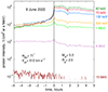 |
Fig. 17. Proton time profiles associated with the IP shock passage on 8 June 2022 representing a plateau response. Legend and lines as in Fig. 13. |
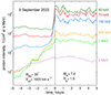 |
Fig. 18. Proton time profiles associated with the IP shock passage on 6 September 2022 representing a plateau response. Legend and lines as in Fig. 13. |
As shown in Table 2, the shock speed (Vsh) is the main IP shock parameter that differentiates the type of the response profile. A previous study by Lario et al. (2005) investigated whether different IP shock parameters, namely the shock speed (Vsh), shock angle (ΘBn), compression ratio (Rmag), and Mach number (MA) were responsible for the different shapes of the proton time profiles associated with the IP shock passage. Those authors found that the fraction of IP shocks showing 47–68 keV ion intensity responses was larger for faster shocks (shown in their Figure 7), however, the shock parameters did not determine unequivocally the type of particle intensity time profile response.
Just as we found for the proton responses ≥6 MeV discussed above, the averaged values also show a noticeable difference in the IP shock parameters for the cases with a plateau response Col. 5 of Table 2. Comparing with the full list of IP shocks with response in protons (Col. 4 of Table 1), these IP shocks are less oblique, namely ⟨ΘBn⟩ = 46° ±10° versus 57° ± 3°, present higher speed, namely ⟨Vsh⟩ = 1083 ± 160 km s−1 versus 547 ± 37 km s−1, exhibit larger Mach numbers (both Alfvénic ⟨MA⟩ = 6.6 ± 0.7 versus 3.8 ± 0.4 and fast magnetosonic ⟨Mfast⟩ = 5.8 ± 0.7 versus 3.1 ± 0.3), higher level of upstream fluctuations, namely ⟨flup⟩ = 0.35 ± 0.09 versus 0.28 ± 0.03, lower upstream density ⟨nup⟩ = 9.7 ± 2.8 versus 20.4 ± 3.6, and lower upstream beta ⟨βup⟩ = 0.61 ± 0.13 versus 0.85 ± 0.13. For comparison, the values of ΘBn identified by Perri et al. (2023) with the magnetic coplanarity method for two out of three IP shocks in their study associated with plateau-type particle profiles were below 70°.
To handle the difference in the radial distance in which an IP shock was observed by the spacecraft, as well as to take into account that the particles accelerated by IP shocks can contain flare-accelerated particles as seed population, especially in case of large events (e.g. Cane et al. 2003; Schwadron et al. 2024), we performed the normalisation procedure described below. For the proton responses classified as plateau and regular peak types we performed a superposed epoch analysis to find an average profile for all events, considering the IP shock passage as ‘zero epoch time’. To improve visibility of each separate event, the normalisation was done dividing the intensity time profiles by the value at the time of the shock passage in the case of regular peak, and by the maximum value in the case of the plateau response. For the analysis, we used for each event the 60 keV energy proton intensity flux at the time of the IP shock passage. We note that due to the low statistics (four events), the plateau response is not very representative, however this type of events is of interest as they are closest to the prediction of DSA theory, as discussed below.
We present in Fig. 19 the result of the superposed epoch analysis for the 12 IP shocks with regular peak proton responses. To make each separate event visible we divided the figure into two parts, each consisting on six events, while the averaged value is calculated from the averaging of all 12 events. The different coloured lines represent the intensity time profiles at 60 keV proton energy for the 12 events as indicated in the legend. There is a strong variety between the individual events, and the mean value ±25% respectively shown in solid and dashed black lines does not cover this variability. Moreover, the different profiles of the different events did not show any ordering in accordance with some of the analysed IP shock parameters, as discussed in Appendix H for the radial distance, shock angle, shock speed, Alfvénic Mach number, compression ratio, and upstream fluctuations.
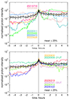 |
Fig. 19. Superposed epoch analysis for the regular peak proton response. The differently coloured curves show the normalised 60 keV proton intensity for the 12 regular types of events, as indicated in the legend. The black solid and black dashed curves represent the mean and ±25% values, respectively. The normalisation was done at each event for the observed proton intensity value at the IP shock front. We divided the figure into two panels for better visualisation. |
Similarly, we show in Fig. 20 the results of the superposed epoch analysis for the plateau response. Here the time profiles represent the predictions of classical DSA in the downstream region, and subsequently the mean value ±25% describes well the events from the time of the sharp increase of the proton intensity until several hours downstream of the IP shock passage. A slight decay after the shock front can be assessed as an effect of adiabatic losses in the downstream region (see e.g. Kartavykh et al. (2016), Afanasiev et al. (2023). For comparison, in Appendix I we show the results of the superposed epoch analysis performed on ESP events observed at 1 au that showed plateau ion response (Lario et al. 2003).
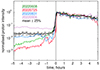 |
Fig. 20. Superposed epoch analysis for the plateau proton response. The normalisation was done at each event for the maximum observed proton intensity value. Legend as in Fig. 19. |
2.3. Comparison of the observed proton profiles with the DSA theory
To understand the role that IP shock parameters play in the formation of the different types of proton responses, we compared for three events their observed and predicted time profiles at several energies under the assumptions of the DSA theory. In the classical one-dimensional steady-state case, one expects to observe a constant proton particle intensity (i.e. a plateau) in the downstream region of the IP shock and an exponential growth towards the IP shock front in the upstream region, in accordance with the following formula (e.g. Drury 1983):
 (3)
(3)
Here U is the speed of the fluid in the upstream region in the de-Hoffmann-Teller frame; z is the distance to the shock (here we consider z = Vsh(t0 − t), with t0 – the time of the shock identification); K is the spatial diffusion coefficient calculated as 1/3λupυ, where υ is the speed of the particles; and λup is the mean free path in the upstream region. Under this formulation, the constant value of the proton intensity in the downstream region is only valid for the plateau type profile. Moreover, in some of the cases where the type regular peak was observed, as was the case for the IP shock on 10 April 2023 shown in Fig. 15, we can see an exponential growth in the upstream part of the profile at the lower energy channels.
Figure 21 shows the time profiles of the proton responses associated with the IP shock on 10 April 2023 in two energy ranges (60 and 130 keV), given in arbitrary units for better visibility of the fitting at each energy range. This IP shock was not strong, with a compression ratio of rgas = 1.7, Alfvénic Mach number of MA = 3.7, and shock speed of ∼500 km s−1, and it was detected very close to the Sun at a heliospheric distance of 0.29 au. The red dashed lines in the figure represent the DSA fitting, which follows well the respective exponential growth of the proton intensities at the two energies shown. The deduced values of the mean free path for this event with the shock speed of 514 km−1 and a fluid speed before the shock passage of 314 km−1 at the respective energies are 0.005 au and 0.0057 au. This result is consistent with the prediction of the quasi-linear theory (QLT) for the energy dependence of the parallel mean free path as ∼E1/6 if the turbulence spectrum is Kolmogorov-like with the spectral index of magnetic fluctuations equal to 5/3 (Jokipii 1966; Hasselmann & Wibberenz 1968).
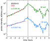 |
Fig. 21. DSA fitting analysis for the IP shock on 10 April 2023. The proton intensities are shown in arbitrary units for the energies of 60 keV and 130 keV, as shown in the legend. The DSA fitting in the upstream region of the shock is indicated by the red dashed curve. Details are given in the main text. |
We further fit the rising part of the intensity time profiles in upstream for two events classified as plateau – the IP shocks on 8 June 2022 and on 6 September 2022 – to identify the mean free paths in the upstream regions under the assumption that they follow the prediction of DSA and the growth rate depends on the value of the parallel diffusion coefficient. Figure 22 shows the fit for the same two energy ranges (60 and 130 keV) for the event of 8 June 2022. The intensity time profiles can be explained for values of the far-upstream mean free path λ|| = 0.013 and 0.0146 au for the energy ranges of 60 and 130 keV, respectively, if one considers the shock speed of 800 km s−1 and the observed fluid speed prior the shock of about 500 km s −1. As for the shock on 10 April 2023, these λ|| values are in agreement with the assumption about the QLT-dependence on energy of the mean free path if the Kolmogorov-like spectrum of turbulence is present. In this case the shock was stronger, with a speed of ∼800 km s−1, with higher Mach numbers and compression ratios (MA = 5, rgas = 2), and it was detected when Solar Orbiter was located at a radial distance of 0.96 au. We note, however, that the time-intensity profile closer to the shock exhibits a super-exponential increase, which would be consistent with the mean free path becoming smaller close to the shock due to generation of foreshock waves generated by streaming instabilities (e.g. Afanasiev et al. 2023). The shock normal angle was also large (ΘBn = 71°), however as discussed below, this is not a necessary condition for creating plateau type responses. We note that the plateau profile was observed only up to 130 keV energies, resembling rather a regular peak response at higher energies (up to 6 MeV). At the energy of ∼15 MeV we found no response, only pre-shock background from the preceding solar energetic particle (SEP) event.
The shock on 6 September 2022 was the fastest one from the list, with a speed of 1600 km s−1, being rather quasi-parallel (ΘBn = 30°). It presented a high Alfvénic Mach number of MA = 7.4, a moderate compression ratio rgas = 1.5, and it was detected at R = 0.7 au. A plateau type response was observed up to 1 MeV energy range, as shown in Fig. 18. Due to a high pre-shock background, it was not possible to get the DSA fit at lower energies (below 500 keV; dark green, red and blue curves in Fig. 18). The beginning of the profile in the energy channel of 500 keV (yellow curve) was also partially affected by the pre-event background level and was not included in the fitting. The results of the fitting for the 1 MeV protons under the assumption of the observed fluid speed of about 400 km s −1 in the upstream region, and of an exponential growth towards the IP shock front with a value of a mean free path of λ|| = 0.013 au is shown in Fig. 23.
The fact that for two plateau type proton enhancements – on 8 June 2022 and 25 July 2022 – where the plateau response was only observed up to 130 keV at 1 au distance, the IP shock speed was ∼800 km s−1, is in favour of the possibility that to achieve a plateau type profile at higher proton energies, a higher IP shock speed would be needed. An example of this possibility are the IP shocks on 31 August 2022 and 6 September 2022, which took place at radial distances of 0.75 au and 0.7 au, respectively and with a speed ≥1000 km s−1, presenting a plateau profile up to 1 MeV proton energies. Therefore, we can conclude that for creating this type of profiles at higher energies, the IP shock speed plays a decisive role, and a value ≥1000 km s−1 is needed, also if the gas compression ratio is ≥1.5.
The acceleration time given by the DSA theory follows the equation below (Drury 1983):
 (4)
(4)
where p is particle momentum; υ its speed; Uup/d are fluid speeds in upstream and downstream; and λup/d is the mean free path in the upstream and downstream regions. This equation means that in case of lower values of the mean free path, as well as for larger compression ratio and Mach numbers in combination with higher shock speed, the acceleration efficiency is also higher, and the plateau scenario can be reached at higher energies, as a steady state at a given energy is achieved earlier with parameters maximising the acceleration rate.
3. Summary and discussion
In this study we analysed energetic particle intensity profiles observed by Solar Orbiter within the time period from April 2020 to April 2023 associated with the passage of IP forward shocks. With this purpose, we used the list of IP shocks compiled by Trotta et al. (2023b, 2025), and the electron and proton fluxes measured by EPT and HET telescopes on board Solar Orbiter. We involved ten IP shock and plasma parameters, as well as information about the radial location of the spacecraft, aiming to understand which parameters determine the particle energisation. These parameters are listed in Table 1, showing the ones used in previous studies, namely shock speed, shock angle (ΘBn), Mach numbers, and several compression ratios; and the parameters not so widely used before, namely the fluctuations of solar wind plasma and magnetic field.
For the analysis of electron acceleration associated with the passage of IP shocks we used three energy ranges: 35.6–63.5 keV, 63.5–121 keV, and 121–238 keV. Taking into account the difficulties on assessing the signal in electron channels around an IP shock passage as being created by electrons, we introduced a parameter that characterises the contamination induced by protons in the electron channels, checked the spectrogram plots and estimated the electron intensity time profiles induced by high-energy (≥20 MeV) protons in electron channels. We found that the acceleration of electrons by IP shocks is rare. As discussed in Sect. 2.1 only in four out of 51 (8%) IP shocks, the electrons showed a response at energies ≤100 keV, and only in one case the shock was able to accelerate electrons up to the energies of 250 keV.
Previous studies by Lario et al. (2003) and Dresing et al. (2016), using measurements exclusively at distances close to 1 au, respectively found electron acceleration efficiencies by IP shocks either higher (17 %) for 45 keV electrons or lower (1%) values for 65–75 keV electrons. The difference in percentages compared to previous studies could be attributed to slightly different energy ranges, with a tendency to observe more events at lower energies, as well as variations in the solar activity level at the time the observations were summarised. Overall, to draw more precise conclusions regarding which shock parameters promote electron acceleration, a larger sample of shocks with a clear identification of the electron response to shock passage is needed. This would likely require a next-generation detector which would allow to separate the electrons and protons unambiguously and which would not suffer from the contamination problem discussed in this paper. Before data from such a detector are available the problem of electron acceleration by interplanetary shocks will remain an open question.
On average, the IP shocks able to accelerate electrons had a larger angle between the shock normal and the direction of the magnetic field in the upstream region, namely ⟨ΘBn⟩ = 68 ± 9° as compared to 54 ± 3° in the sample of IP shocks used for the search for electron acceleration in this study. This corresponds to an IP shock geometry closer to quasi-perpendicular, suggesting that the SDA mechanism, namely when the energy gain is due to the electric field, is preferential for the electron energisation, as electrons have much smaller masses in comparison with protons. We do not find a difference in the shock speed of the IP shocks which are able to accelerate electrons: 545 ± 81 km s −1 for the restricted electron-response sample versus 512 ± 24 km s−1 for the sample of IP shocks used for comparison. This is also in favour of the SDA (or stochastic SDA) mechanism being responsible for the electron energisation. A similar study performed by Liu et al. (2022) based on data from the Wind spacecraft and related to the Earth’s bow shock revealed that the majority of the electrons in the energy range ∼0.5–∼100 keV were in regions where the shock geometry was close to 90°, supporting the scenario of SDA (or stochastic SDA) for energetic electrons.
Based on the detailed analysis of the four IP shocks which were able to accelerate electrons as presented in Sect. 2.1, we suggest that the acceleration mechanism behind the energisation of the electrons is most likely SDA (or stochastic SDA), and in some cases multiple SDA-like interactions with multiple shocks. This latter scenario of multiple SDA was found to take place for shocks with rather oblique geometry, or in the case of a sequence of several IP shock structures approaching each other and bouncing electrons between them. The ability of oblique shocks to reflect electrons when they propagate from upstream to downstream was also confirmed by the observations in connection with IP shocks (e.g. Wilson 2009) and with the Earth’s bow shock (e.g. Kartavykh et al. 2013).
For the analysis of proton acceleration associated with the passage of IP shocks, we used seven proton energy channels, from 60 keV up to 15 MeV. Using a reference energy of 100 keV, we found 40 out of 48 (83%) IP shocks which are associated with a proton response, as shown in Col. 4 of Table 1. The probability of acceleration by IP shocks presented in Fig. 12 shows that the higher the proton energy, the smaller the number of observed IP shocks being able to produce a response. The total number of IP shocks where protons with energies ≥100 keV produced a response was 40 (including the 16 IP shocks listed in Table 2 where only protons with energies ≤100 keV showed some increase). However, there were only eight IP shocks which affected the time profiles of protons with energies ≥6 MeV, and only four shocks (two of them had a plateau type of response, and two were connected with a sequence of several shocks, which are more efficient; see e.g. Niemela et al. 2024) where a response at an energy of 15 MeV was noticeable. A similar tendency, namely that the larger the proton energy the smaller the number of IP shocks with response at this energy is confirmed by Trotta et al. (2025) for a larger set of shocks observed by Solar Orbiter. Based on the results shown in Table 2, the ability to accelerate protons to higher energies mostly depends on the IP shock speed. The importance of the IP shock transit speed in accelerating protons to higher energies was also found by Ameri et al. (2023).
We identified six different proton response shapes associated with the IP shock passage. Based on the response at low energies of ∼100 keV, we divided the profiles into no response, weak response, peak (regular or irregular), plateau, and unclear response. As shown in Table 2, we found that the ability to form a particular shape of the particle response to the IP shock passage also mainly depends on the IP shock speed. Weak, regular peak, and plateau responses were respectively found for an IP shock mean speed of 462 ± 20 km s−1, 556 ± 38 km s−1, and 1083 ± 160 km s−1. We also found that the response of the time profiles is energy-dependent. The strength of an IP shock could be enough to achieve a plateau response at lower proton energies, while at high proton energies the profiles would correspond to the regular peak type.
A plateau response was found in 4 out of 48 (8%) cases, as shown in Col. 5 of Table 2 and is therefore as rare as those shocks with an electron response. As discussed above, this profile is characterised by a much higher IP mean shock speed, namely 1083 ± 160 km s−1 compared to the 547 ± 37 km s−1, and a higher gas compression ratio rg, namely 2.4 ± 0.4 versus 2.0 ± 0.1 found for the 40 IP shocks with response in protons, presented in Col. 5 of Table 1. In the plateau profile, we found a smaller mean value of the shock angle – 46 ± 10° compared to 57 ± 3° – and a higher mean level of upstream fluctuations, 0.35 ± 0.04 compared to 0.28 ± 0.03. The mean ratio between the downstream and upstream fluctuation levels was close to 1.0, namely 1.08 ± 0.04 compared to 1.33 ± 0.08. A ratio close to 1.0 would mean that also in the downstream region the mean free path is small enough to allow developing a situation close to classical DSA.
At energies exceeding a shock-specific threshold (e.g. ≥5 MeV) the response is different from the prediction of the classical DSA. At these energies the response is primarily due to the reflection of particles at the shock. This shock-specific threshold is shifted to higher energies with increasing shock speed, Vsh. Therefore shock speed is an important parameter when considering IP shocks.
We further suggest that the regular peak and plateau responses represent two stages of DSA at the IP shock. The first stage, namely the regular peak, corresponds to the phase when DSA produced an exponential growth in the upstream region towards the IP shock front, however the conditions are not favourable to achieve the equilibrium state in the downstream region. In addition to shock strength and speed, the extent of the upstream region can play a decisive role in achieving the prediction of classical DSA theory (e.g. Kartavykh et al. 2016). The identified energy dependence of the far-upstream parallel mean free path corresponds to the predictions given by QLT, coinciding with the results obtained by Giacalone et al. (2023) for the ESP event on 16 February 2022 observed by Parker Solar Probe Fox et al. (2016) up to ∼750 keV. We note, however, that some of the plateau-type events show super-exponential increases close to the shock that can be interpreted as evidence for generation of foreshock turbulence by the streaming energetic particles themselves (Afanasiev et al. 2023).
The plateau type response reflects the classical prediction of DSA, when the mean free path is small enough so that the intensity in the downstream region is constant. In the upstream region one can expect an exponential growth in intensity towards the downstream region (e.g. Drury 1983) shown in Equation (3). We suggest that the plateau response to the passage of an IP shock might be related with a high IP shock speed, relatively large gas compression ratio (Rgas ≥ 1.5), and a small mean free path around the IP shock front of ≤0.02 au. We note that the plateau type shocks under study were observed at radial distances ≥0.7 au. Taking into account the importance of acceleration time one can expect that closer to the Sun the compression ratio can be larger and, opposite, the mean free path smaller, to achieve the same effect.
The role of the IP shock speed in the formation of the proton response to the shock makes a difference in comparison with the classical DSA theory, where the decisive role is given by the compression ratio. The reason of this difference is that opposite to the classical case, where the whole structure is infinite and static, the IP shocks are objects moving with a finite speed, and the acceleration time is limited by the propagation time of the shocks. As one can see from Eq. (4) the acceleration time gets smaller the larger the difference is between the fluid speeds in upstream and downstream, and the values of the fluid speeds in both regions. Large values of these parameters can only be obtained when the shock speed is high and the compression ratio is large enough (at least above 1.5). Therefore, the important role of the shock speed in the formation of proton time profile is directly connected with the main feature of IP shocks as fast moving objects.
4. Conclusions
Our main conclusions can be summarised as follows:
Future observations of an individual IP shock performed by two or more spacecraft (e.g. Lario et al. 2019; Khoo et al. 2024; Trotta et al. 2024b) along with the accompanying particles will be crucial in understanding how the particle response evolves in time and how it changes as a function of the shock strength and geometry. A combination of more realistic models of the interaction of particles with the shock front and the turbulence in a self-consistent manner with such observations could improve our understanding of shock accelerationmechanisms.
Acknowledgments
This work has received funding by the European Union’s Horizon 2020 research and innovation program under grant agreement No. 101004159 (SERPENTINE). The paper reflects only the authors’ view and the European Commission is not responsible for any use that may be made of the information it contains. Y.K. and W.D. acknowledge support by the International Space Science Institute (ISSI) in Bern and Beijing, through ISSI/ISSI-BJ International Team project ‘Understanding the Release of Hard X-Rays, Type III Radio Bursts and In-Situ Electrons in Solar Flares’ (ISSI Team project 23-581; ISSI-BJ Team project 56). L.R.-G. acknowledges support through the European Space Agency (ESA) research fellowship programme. AK and RFWS thank the German Space Agency (DLR) for its support of Solar Orbiter’s EPD under grant 50 OT 2002. JRP, FEL, and RGH acknowledge Spanish MINCIN Project PID2019-104863RBI00/AEI/10.13039/501100011033. N.D. acknowledges funding by the Research Council of Finland (SHOCKSEE, grant No. 346902). R.V. and E.K. gratefully acknowledge funding by the Research Council of Finland for the Finnish Centre of Excellence in Research of Sustainable Space (FORESAIL, grant No. 352847 and 352850). The UAH team has been funded by MICIU/AEI and FEDER, UE under project PID2023-150952OB-I00/10.13039/501100011033. D.L. acknowledges support from NASA Living With a Star (LWS) program NNH19ZDA001N-LWS, and the Guest Investigator Program NNH23ZDA001N-HGIO. Solar Orbiter magnetometer operations are funded by the UK Space Agency (grant ST/X002098/1). T.H. is supported by STFC grant ST/W001071/1.
References
- Afanasiev, A., Vainio, R., Trotta, D., et al. 2023, A&A, 679, A111 [CrossRef] [EDP Sciences] [Google Scholar]
- Amano, T., Katou, T., Kitamura, N., et al. 2020, Phys. Rev. Lett., 124, 065101 [NASA ADS] [CrossRef] [Google Scholar]
- Amano, T., Masuda, M., Oka, M., et al. 2024, Phys. Plasmas, 31, 042903 [Google Scholar]
- Ameri, D., Valtonen, E., Al-Sawad, A., & Vainio, R. 2023, Adv. Space Res., 71, 2521 [NASA ADS] [CrossRef] [Google Scholar]
- Bryant, D. A., Cline, T. L., Desai, U. D., & McDonald, F. B. 1962, J. Geophys. Res., 67, 4983 [NASA ADS] [CrossRef] [Google Scholar]
- Bryant, D. A., Cline, T. L., Desai, U. D., & McDonald, F. B. 1965, ApJ, 141, 478 [Google Scholar]
- Cane, H. V., von Rosenvinge, T. T., Cohen, C. M. S., & Mewaldt, R. A. 2003, Geophys. Res. Lett., 30, 8017 [NASA ADS] [Google Scholar]
- Decker, R. B. 1983, J. Geophys. Res., 88, 9959 [Google Scholar]
- Dresing, N., Theesen, S., Klassen, A., & Heber, B. 2016, A&A, 588, A17 [NASA ADS] [CrossRef] [EDP Sciences] [Google Scholar]
- Drury, L. O. 1983, Reports on Progress in Physics, 46, 973 [Google Scholar]
- Fox, N. J., Velli, M. C., Bale, S. D., et al. 2016, Space Sci. Rev., 204, 7 [Google Scholar]
- Giacalone, J., Cohen, C. M. S., McComas, D. J., et al. 2023, ApJ, 958, 144 [NASA ADS] [CrossRef] [Google Scholar]
- Gieseler, J., Dresing, N., Palmroos, C., et al. 2023, Front. Astron. Space Sci., 9, 384 [NASA ADS] [CrossRef] [Google Scholar]
- Gold, R. E., Krimigis, S. M., Hawkins, S. E. I., et al. 1998, Space Sci. Rev., 86, 541 [Google Scholar]
- Hasselmann, K., & Wibberenz, G. 1968, Zeitshrift fuer Geophysik, 34, 353 [Google Scholar]
- Hietala, H., Trotta, D., Fedeli, A., et al. 2024, MNRAS, 531, 2415 [NASA ADS] [Google Scholar]
- Huttunen-Heikinmaa, K., & Valtonen, E. 2005, in 29th International Cosmic Ray Conference (ICRC29), Volume 1, Int. Cosmic Ray Conf., 1, 59 [Google Scholar]
- Jebaraj, I. C., Dresing, N., Krasnoselskikh, V., et al. 2023, A&A, 680, L7 [NASA ADS] [CrossRef] [EDP Sciences] [Google Scholar]
- Jokipii, J. R. 1966, ApJ, 146, 480 [Google Scholar]
- Kaiser, M. L., Kucera, T. A., Davila, J. M., et al. 2008, Space Sci. Rev., 136, 5 [Google Scholar]
- Kallenrode, M.-B. 1996, J. Geophys. Res., 101, 24393 [Google Scholar]
- Kartavykh, Y. Y., Dröge, W., & Klecker, B. 2013, J. Geophys. Res. (Space Phys.), 118, 4005 [Google Scholar]
- Kartavykh, Y. Y., Dröge, W., & Gedalin, M. 2016, ApJ, 820, 24 [Google Scholar]
- Katou, T., & Amano, T. 2019, ApJ, 874, 119 [NASA ADS] [CrossRef] [Google Scholar]
- Khoo, L. Y., Sánchez-Cano, B., Lee, C. O., et al. 2024, ApJ, 963, 107 [NASA ADS] [CrossRef] [Google Scholar]
- Kilpua, E., Vainio, R., Cohen, C., et al. 2023, Ap&SS, 368, 66 [NASA ADS] [CrossRef] [Google Scholar]
- Koval, A., & Szabo, A. 2008, J. Geophys. Res. (Space Phys.), 113, A10110 [NASA ADS] [CrossRef] [Google Scholar]
- Krymskii, G. F. 1977, Akademiia Nauk SSSR Doklady, 234, 1306 [NASA ADS] [Google Scholar]
- Lario, D., Ho, G. C., Decker, R. B., et al. 2003, in Solar Wind Ten, eds. M. Velli, R. Bruno, F. Malara, & B. Bucci, (AIP), AIP Conf. Ser., 679, 640 [NASA ADS] [CrossRef] [Google Scholar]
- Lario, D., Hu, Q., Ho, G. C., et al. 2005, in Solar Wind 11/SOHO 16, Connecting Sun and Heliosphere, eds. B. Fleck, T. H. Zurbuchen, & H. Lacoste, ESA Spec. Pub., 592, 81 [Google Scholar]
- Lario, D., Berger, L., Decker, R. B., et al. 2019, AJ, 158, 12 [NASA ADS] [CrossRef] [Google Scholar]
- Liu, Z., Wang, L., & Guo, X. 2022, ApJ, 935, 39 [NASA ADS] [CrossRef] [Google Scholar]
- Müller, D., St. Cyr, O. C., Zouganelis, I., et al. 2020, A&A, 642, A1 [Google Scholar]
- Niemela, A., Wijsen, N., Aran, A., et al. 2024, ApJ, 967, L35 [Google Scholar]
- Paschmann, G., & Schwartz, S. J. 2000, in ISSI Book on Analysis Methods for Multi-Spacecraft Data (ESA), ESA Spec. Pub., 449, 99 [Google Scholar]
- Perri, S., Prete, G., Zimbardo, G., et al. 2023, ApJ, 950, 62 [Google Scholar]
- Rodríguez-Pacheco, J., Sequeiros, J., Del Peral, L., Bronchalo, E., & Cid, C. 1998, Sol. Phys., 181, 185 [CrossRef] [Google Scholar]
- Rodríguez-Pacheco, J., Wimmer-Schweingruber, R. F., Mason, G. M., et al. 2020, A&A, 642, A7 [Google Scholar]
- Sandroos, A., & Vainio, R. 2006, A&A, 455, 685 [NASA ADS] [CrossRef] [EDP Sciences] [Google Scholar]
- Schwadron, N. A., Bale, S. D., Bonnell, J., et al. 2024, ApJ, 970, 98 [Google Scholar]
- Stone, E. C., Frandsen, A. M., Mewaldt, R. A., et al. 1998, Space Sci. Rev., 86, 1 [Google Scholar]
- Trotta, D., Vuorinen, L., Hietala, H., et al. 2022, Front. Astron. Space Sci., 9, 1005672 [NASA ADS] [CrossRef] [Google Scholar]
- Trotta, D., Hietala, H., Horbury, T., et al. 2023a, MNRAS, 520, 437 [NASA ADS] [CrossRef] [Google Scholar]
- Trotta, D., Horbury, T., Dresing, N., et al. 2023b, SERPENTINE D4.3: List of in-situ shock parameters, Cycle 25, version 1, Tech. rep., Imperial College London [Google Scholar]
- Trotta, D., Horbury, T. S., Lario, D., et al. 2023c, ApJ, 957, L13 [CrossRef] [Google Scholar]
- Trotta, D., Hietala, H., Dresing, N., et al. 2024a, Solar Orbiter Cycle 25 Interplanetary Shock List, http://dx.doi.org/10.5281/zenodo.12518015 [Google Scholar]
- Trotta, D., Larosa, A., Nicolaou, G., et al. 2024b, ApJ, 962, 147 [CrossRef] [Google Scholar]
- Trotta, D., Dimmock, A. P., Blanco-Cano, X., et al. 2024c, ApJ, 971, L35 [Google Scholar]
- Trotta, D., Dimmock, A., Hietala, H., et al. 2025, ApJS, 277, 2 [Google Scholar]
- Tsurutani, B. T., & Lin, R. P. 1985, J. Geophys. Res., 90, 1 [NASA ADS] [CrossRef] [Google Scholar]
- Wilson, L. B. I., Cattell, C. A., Kellogg, P. J., et al. 2009, J. Geophys. Res. (Space Phys.), 114, A10106 [Google Scholar]
- Wimmer-Schweingruber, R. F., Janitzek, N. P., Pacheco, D., et al. 2021, A&A, 656, A22 [NASA ADS] [CrossRef] [EDP Sciences] [Google Scholar]
- Wraase, S., Heber, B., Böttcher, S., et al. 2018, A&A, 611, A100 [NASA ADS] [CrossRef] [EDP Sciences] [Google Scholar]
- Yang, L., Heidrich-Meisner, V., Berger, L., et al. 2023, A&A, 673, A73 [NASA ADS] [CrossRef] [EDP Sciences] [Google Scholar]
Appendix A: Averaged parameters for all forward shocks and for which all parameters were known
We include in Table A.1 the average, median, and standard error values of the IP shock parameters for the total number of forward IP shocks included in this study (Col. 2), and for the forward IP shocks where all parameters are known (Col. 3).
Parameters of forward shocks under study, and of the forward shocks where all parameters were known. a
Appendix B: Contamination by high-energy protons
Figure B.1 shows a particle enhancement in connection with the shock on 31 August 2022. Taking into account the contamination parameter a peak after the shock might be connected with electrons, but observations by HET high-energy protons lead to the conclusion that in reality these are protons counted in electron channel (Fig. B.1). Similarly the peak at low electron energies after the shock on 26 December 2022 could be partially created by real electrons because the contamination parameter was lower than 0.6, but after simulation a response in EPT due to high-energy protons observed by HET forced us to reject this case completely as being produced by the effect of protons above 20 MeV (see Fig. B.2). Additionally we show the spectrogram plots for these two events (Figs. B.3 and B.4).
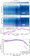 |
Fig. B.1. Particle response to the IP shock on 31 August 2022 with ΘBn = 22°, Vsh = 1100 km s−1. From top to bottom: Measured count rate in the foil Sun detector, calculated count rate in the foil Sun detector, count rate in energy channels 10-14 as a function of time, count rate spectrum for the period of time indicated as "tp1" in the top two panels. |
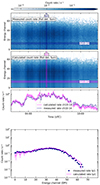 |
Fig. B.2. Particle response to the IP shock on 26 December 2022 with ΘBn = 71°, Vsh = 598 km s−1. From top to bottom: Measured count rate in foil Sun detector, calculated count rate in foil Sun detector, count rate in energy channels 10-14 as a function of time, count rate spectrum for the period of time indicated as "tp1" in the top two panels. |
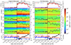 |
Fig. B.3. Particle response to the IP shock on 31 August 2022. Legend and panel description as in Fig. 2. |
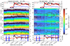 |
Fig. B.4. Particle response to the IP shock on 26 December 2022 (no electrons). Legend and panel description as in Fig. 2. |
Appendix C: Particle response around the 27 November 2021 IP shock
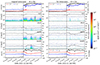 |
Fig. C.1. Particle response to the IP shock on 27 November 2021. Legend and panel description as in Fig. 2. |
Figure C.1 shows the directional information of the 27 November 2021 event. The electron increase was observed after the shock passage, but it exhibited a clear solar direction. Solar Orbiter was located close to the Earth after the gravity assist manoeuvrer and it could be well magnetically connected to the magnetosphere or to the bow shock. Therefore, this event was removed from the sample out of caution.
Appendix D: Particle increase around the 9 March 2022 IP shock
The spectrogram of particle data around the IP shock observed on 9 March 2022 at 14:48:32 UT is shown in Figure D.1.
The IP shock exhibited Mach numbers of 1.9 (Alfvénic) and 1.6 (fast magnetosonic), a shock speed of 430 km s−1, and values of 1.4 and 1.6, respectively, for magnetic and gas compression ratios. The value of the shock normal angle was ΘBn = 70°, which corresponds to a quasi-perpendicular IP shock. The IP shock on 9 March 2022 was observed closely in time when several solar flares classified as ∼ B5 in flux intensity had accelerated electrons mainly up to the energies of ≤ 100 keV (one of the flares happened at 14:01:10 UT). One can see a clear velocity dispersion in electron data on the spectrogram plot, suggesting solar origin of these peak.
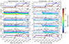 |
Fig. D.1. Particle response to the IP shock on 9 March 2022. Legend and panel description as in Fig. 2. |
Appendix E: Particle increase around the 13 January 2023 IP shock
The particle response to the IP shock on 13 January 2023 is shown on Figs. E.1 and E.2. One can see on the spectrogram a clear velocity dispersion suggesting solar origin of electrons coming after the shock.
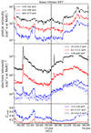 |
Fig. E.1. Particle response to the IP shock on 13 January 2023 with ΘBn = 52°, Vsh = 473 km s−1. From top to bottom: Time profile of protons, electrons (solid line - uncorrected, dotted line - corrected), and Ccont parameter. The legend shows the different energy channels used following the colour code. The vertical solid line indicates the IP shock arrival. |
 |
Fig. E.2. Particle response to the IP shock on 13 January 2023 (no electrons). Legend and panel description as in Fig. 2. |
Appendix F: Particle response around fast IP shock passage of type plateau
We show here particle data in the vicinity of the shock on 8 June 2022 (ΘBn = 71°, Vsh = 812 km s−1), classified as plateau type in accordance with proton time profiles (Fig. F.1). One can clearly see a contamination by protons in electron channel, and therefore one cannot asses this case as an electron response.
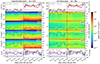 |
Fig. F.1. Particle response to the IP shock on 8 June 2022. Legend and panel description as in Fig. 2. |
Appendix G: Proton response additional profiles: Irregular peak and unclear response
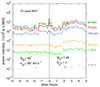 |
Fig. G.1. Proton time profiles associated with the IP shock passage on 13 June 2021 representing an irregular peak response. Legend and lines as in Fig. 13. |
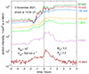 |
Fig. G.2. Proton time profiles associated with the IP shock passage on 3 November 2021 at 14:04 UT representing an irregular peak response. Legend and lines as in Fig. 13. |
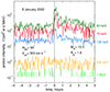 |
Fig. G.3. Proton time profiles associated with the IP shock passage on 8 January 2022 at 14:04 UT representing an irregular peak response. Legend and lines as in Fig. 13. |
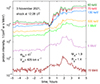 |
Fig. G.4. Proton time profiles associated with the IP shock passage on 3 November 2021 at 12:28 UT representing an unclear response. Legend and lines as in Fig. 13. |
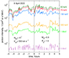 |
Fig. G.5. Proton time profiles associated with the IP shock passage on 8 April 2022 representing an unclear response. Legend and lines as in Fig. 13. |
We classified as an irregular peak profile the proton responses to the IP shocks on 13 2021 June 2021 (G.1), 3 November 2021 (at 14:04 UT), 8 January 2022, and 3 July 2022. The shock on 13 June 2021 (at 10:08:38 UT) was neither fast nor strong: (Vsh = 387 km s−1, Rgas = 1.7, RB = 1.5, MA = 1.45, Mfast = 1.3. The identified shock angle was close to 90 degrees (ΘBn = 82°). The peak was small, and the whole profile exhibited an irregular shape. We discuss here two of the shocks which show a particular behaviour. The IP shock on 3 November 2021 at 14:04 UT (Fig. G.2) was the third in a sequence of IP shocks. By itself it was not a particularly strong shock: Rgas = 2.2, RB = 1.9, MA = 3.2, Mfast = 2.9, Vsh = 502 km s −1 and ΘBn = 42°. The IP shock on 8 January 2022 (Fig. G.3) was strong based on the magnetic compression ratio (RB = 3.3), and Mach numbers (MA = 10.3, Mfast = 6), but it was rather slow (Vsh = 303 km s −1) and had a low value of the gas compression ratio (Rgas = 1.8). The shock angle was ΘBn = 64°. All together it did not lead to an efficient particle acceleration.
We classified as unclear peak profiles the proton responses to the IP shocks on 3 November 2021 (12:28 UT), 27 November 2021 (22:29:45 UT), and 8 April 2022. We discuss here two of them which show some particular behaviour. As already discussed in the main text, on 3 November 2021 a sequence of three IP shocks was observed by Solar Orbiter. The shock arriving at 12:28 UT was the second one of the sequence (Fig. G.4). It exhibited a shock angle ΘBn = 41° and it was not strongly based on the compression ratios (RB and Rgas= 1.4), Mach number (MA = 1.9, Mfast = 1.8), and the shock speed was Vsh = 426 km s −1. The IP shock detected on 8 April 2022 (Fig. G.5), had a shock angle of ΘBn = 41°, speed Vsh = 530 km s −1, relatively high Mach numbers (MA = 6.6, Mfast = 6.2), and modest compression ratios (RB = 2.5, Rgas = 1.5). Apparently the shock affected the intensity time profiles of protons up to 1 MeV, but neither formed a clear peak nor a plateau.
Appendix H: Superposed regular peak as a function of the IP shock parameters
Figures H.1–H.6, respectively, show that the superposed epoch analysis of the regular peak proton responses of the 12 different events did not show any ordering in accordance with the following IP shock parameters: radial distance, shock angle, shock speed, Alfvénic Mach number, compression ratio, and upstream fluctuations.
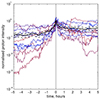 |
Fig. H.1. Superposed epoch analysis for the regular peak response. Legend as in Fig. 19, with the coloured lines representing larger radial distance when the colour is closer to blue. |
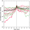 |
Fig. H.2. Superposed epoch analysis for the regular peak response. Legend as in Fig. 19, with the coloured lines representing larger larger shock angle when the colour is closer to red. |
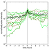 |
Fig. H.3. Superposed time profile analysis for the regular peak response. Legend as in Fig. 19, with the coloured lines representing higher shock speed when the colour is closer to green. |
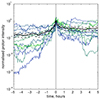 |
Fig. H.4. Superposed epoch analysis for the regular peak response. Legend as in Fig. 19, with the coloured lines representing larger Alfvénic Mach numbers when the colour is closer to green. |
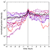 |
Fig. H.5. Superposed epoch analysis for the regular peak response. Legend as in Fig. 19, with the coloured lines representing higher compression ratio when the colour is closer to red and lower when closer to blue. |
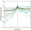 |
Fig. H.6. Superposed epoch analysis for the regular peak response. Legend as in Fig. 19, with the coloured lines representing larger level of upstream fluctuations when the colour is closer to blue. |
Appendix I: Superposed epoch analysis for plateau type based on ACE observations
Figure I.1 shows the superposed epoch analyses for those ESP events analysed by Lario et al. (2003) displaying a plateau response (or ‘classic ESP event’ in the terminology used by Lario et al. 2003) and showing an increase in the 1.9-4.8 MeV ion intensities measured by the Low Energy Magnetic Spectrometer (LEMS) telescope telescope of the EPAM –Gold et al. (1998)– on board ACE. Since all these ESP events were measured at the Sun-Earth Lagrangian point L1, no normalisation was applied, and the coloured curves in panels (a-c) show the ion intensities of each individual event as directly measured by ACE/EPAM/LEMS120 whereas the thick lines in panels (a)-(c) of Fig. I.1 provide the averaged intensity of this type of events measured at 1 au.
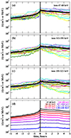 |
Fig. I.1. Superposed epoch analysis for the ESP events analysed by Lario et al. (2003) showing a plateau response. The different coloured curves in panels (a-c) show the ion intensities at three different energies as measured by ACE/EPAM/LEMS120 for the 18 ESP events classified as classic-ESP events by Lario et al. (2003) that showed an increase in the 1.9-4.8 MeV ion intensities. The thick black curves represent the mean intensities. The different curves in panel (d) show the average intensity for these 18 events at the different energy channels of ACE/EPAM/LEMS120. The vertical black line identifies the shock passage. |
All Tables
Shock parameters (Trotta et al. 2024a) with and without electron and proton response.
Parameters of forward shocks under study, and of the forward shocks where all parameters were known. a
All Figures
|
Fig. 1. Particle response to the IP shock on 22 August 2021 with ΘBn = 88°. From top to bottom the panels show the time profile of protons, electrons (solid line – uncorrected, dotted line – corrected), and Ccont. The insets show the colour-coding used for the different energy channels. The vertical solid line indicates the IP shock arrival. Rsc = 0.65 au. |
| In the text | |
|
Fig. 2. Particle response to the IP shock on 22 August 2021. Top panel: Solar wind speed (black curve, left axis), solar wind temperature (red curve, right axis, kT), solar wind number density (blue curve, right axis). Middle four panels: EPT foil (left) and magnet (right) observations by Solar Orbiter from different telescopes, as indicated in the upper right corner of each panel. The pitch angle is shown as a dot-dashed line (right axis). The colour bar on the right shows the intensity. Bottom panel: Magnetic field magnitude ∣B∣ (black curve, left axis), and polar (red curve, right axis) and azimuthal (blue curve, right axis) angles. The vertical dashed line indicates the IP shock arrival. |
| In the text | |
|
Fig. 3. Constellation of spacecraft at the time of the shock passing Solar Orbiter at 14:04 UT. |
| In the text | |
|
Fig. 4. Proton time profiles and corrected electron time profiles associated with the IP shock passage on 3 November 2021 at 14:04 UT. The energy ranges are given in the legend. Rsc = 0.42 au. |
| In the text | |
|
Fig. 5. Particle response to the IP shock on 3 November 2021 at 14:04 UT. From top to bottom: Measured count rate in foil Sun detector, calculated count rate in foil Sun detector, count rate in energy channels 10–14 as a function of time, count rate spectrum for the period of time indicated as “tp1” in the top two panels. |
| In the text | |
|
Fig. 6. Particle response to the IP shock on 3 November 2021. Legend and panel description as in Fig. 2. |
| In the text | |
|
Fig. 7. Electron response to the IP shock on 21 May 2022 with ΘBn = 80°. Description and legend as in Fig. 1. |
| In the text | |
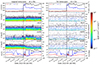 |
Fig. 8. Particle response to the IP shock on 21 May 2022. Legend and panel description as in Fig. 2. |
| In the text | |
|
Fig. 9. Proton time profiles (lines) and corrected electron time profiles (dots) associated with the IP shock passage on 25 July 2022. The energy ranges are given in the legend. |
| In the text | |
|
Fig. 10. Particle response to the IP shock on 25 July 2022. From top to bottom: Measured count rate in the foil Sun detector, calculated count rate in foil Sun detector, count rate in energy channels 10–14 as a function of time, count rate spectrum for the period of time indicated as “tp1” in the top two panels. |
| In the text | |
|
Fig. 11. Particle response to the IP shock on 25 July 2022. Legend and panel description as in Fig. 2. |
| In the text | |
|
Fig. 12. Probability of acceleration as a function of proton energy. The energy intervals are indicated by the horizontal error bars, and the standard error by the vertical error bars. E0 = 1 MeV. Details are given in the main text. |
| In the text | |
|
Fig. 13. Proton time profiles associated with the IP shock passage (vertical line) on 23 October 2021 representing a weak response. The different energy ranges are indicated by the coloured lines (see legend on the right). |
| In the text | |
|
Fig. 14. Proton time profiles associated with the IP shock passage on 13 May 2022 representing a regular peak response. Legend and lines as in Fig. 13. |
| In the text | |
|
Fig. 15. Proton time profiles associated with the IP shock passage on 10 April 2023 representing a regular peak response. Legend and lines as in Fig. 13. |
| In the text | |
|
Fig. 16. Proton time profiles associated with the IP shock passage on 30 August 2022 representing a regular peak response. Legend and lines as in Fig. 13. |
| In the text | |
|
Fig. 17. Proton time profiles associated with the IP shock passage on 8 June 2022 representing a plateau response. Legend and lines as in Fig. 13. |
| In the text | |
|
Fig. 18. Proton time profiles associated with the IP shock passage on 6 September 2022 representing a plateau response. Legend and lines as in Fig. 13. |
| In the text | |
|
Fig. 19. Superposed epoch analysis for the regular peak proton response. The differently coloured curves show the normalised 60 keV proton intensity for the 12 regular types of events, as indicated in the legend. The black solid and black dashed curves represent the mean and ±25% values, respectively. The normalisation was done at each event for the observed proton intensity value at the IP shock front. We divided the figure into two panels for better visualisation. |
| In the text | |
|
Fig. 20. Superposed epoch analysis for the plateau proton response. The normalisation was done at each event for the maximum observed proton intensity value. Legend as in Fig. 19. |
| In the text | |
|
Fig. 21. DSA fitting analysis for the IP shock on 10 April 2023. The proton intensities are shown in arbitrary units for the energies of 60 keV and 130 keV, as shown in the legend. The DSA fitting in the upstream region of the shock is indicated by the red dashed curve. Details are given in the main text. |
| In the text | |
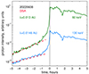 |
Fig. 22. DSA fitting analysis for the IP shock on 8 June 2022. Legend as in Fig. 21. |
| In the text | |
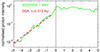 |
Fig. 23. DSA fitting analysis for the IP shock on 6 September 2022. Legend as in Fig. 21. |
| In the text | |
|
Fig. B.1. Particle response to the IP shock on 31 August 2022 with ΘBn = 22°, Vsh = 1100 km s−1. From top to bottom: Measured count rate in the foil Sun detector, calculated count rate in the foil Sun detector, count rate in energy channels 10-14 as a function of time, count rate spectrum for the period of time indicated as "tp1" in the top two panels. |
| In the text | |
|
Fig. B.2. Particle response to the IP shock on 26 December 2022 with ΘBn = 71°, Vsh = 598 km s−1. From top to bottom: Measured count rate in foil Sun detector, calculated count rate in foil Sun detector, count rate in energy channels 10-14 as a function of time, count rate spectrum for the period of time indicated as "tp1" in the top two panels. |
| In the text | |
|
Fig. B.3. Particle response to the IP shock on 31 August 2022. Legend and panel description as in Fig. 2. |
| In the text | |
|
Fig. B.4. Particle response to the IP shock on 26 December 2022 (no electrons). Legend and panel description as in Fig. 2. |
| In the text | |
|
Fig. C.1. Particle response to the IP shock on 27 November 2021. Legend and panel description as in Fig. 2. |
| In the text | |
|
Fig. D.1. Particle response to the IP shock on 9 March 2022. Legend and panel description as in Fig. 2. |
| In the text | |
|
Fig. E.1. Particle response to the IP shock on 13 January 2023 with ΘBn = 52°, Vsh = 473 km s−1. From top to bottom: Time profile of protons, electrons (solid line - uncorrected, dotted line - corrected), and Ccont parameter. The legend shows the different energy channels used following the colour code. The vertical solid line indicates the IP shock arrival. |
| In the text | |
|
Fig. E.2. Particle response to the IP shock on 13 January 2023 (no electrons). Legend and panel description as in Fig. 2. |
| In the text | |
|
Fig. F.1. Particle response to the IP shock on 8 June 2022. Legend and panel description as in Fig. 2. |
| In the text | |
|
Fig. G.1. Proton time profiles associated with the IP shock passage on 13 June 2021 representing an irregular peak response. Legend and lines as in Fig. 13. |
| In the text | |
|
Fig. G.2. Proton time profiles associated with the IP shock passage on 3 November 2021 at 14:04 UT representing an irregular peak response. Legend and lines as in Fig. 13. |
| In the text | |
|
Fig. G.3. Proton time profiles associated with the IP shock passage on 8 January 2022 at 14:04 UT representing an irregular peak response. Legend and lines as in Fig. 13. |
| In the text | |
|
Fig. G.4. Proton time profiles associated with the IP shock passage on 3 November 2021 at 12:28 UT representing an unclear response. Legend and lines as in Fig. 13. |
| In the text | |
|
Fig. G.5. Proton time profiles associated with the IP shock passage on 8 April 2022 representing an unclear response. Legend and lines as in Fig. 13. |
| In the text | |
|
Fig. H.1. Superposed epoch analysis for the regular peak response. Legend as in Fig. 19, with the coloured lines representing larger radial distance when the colour is closer to blue. |
| In the text | |
|
Fig. H.2. Superposed epoch analysis for the regular peak response. Legend as in Fig. 19, with the coloured lines representing larger larger shock angle when the colour is closer to red. |
| In the text | |
|
Fig. H.3. Superposed time profile analysis for the regular peak response. Legend as in Fig. 19, with the coloured lines representing higher shock speed when the colour is closer to green. |
| In the text | |
|
Fig. H.4. Superposed epoch analysis for the regular peak response. Legend as in Fig. 19, with the coloured lines representing larger Alfvénic Mach numbers when the colour is closer to green. |
| In the text | |
|
Fig. H.5. Superposed epoch analysis for the regular peak response. Legend as in Fig. 19, with the coloured lines representing higher compression ratio when the colour is closer to red and lower when closer to blue. |
| In the text | |
|
Fig. H.6. Superposed epoch analysis for the regular peak response. Legend as in Fig. 19, with the coloured lines representing larger level of upstream fluctuations when the colour is closer to blue. |
| In the text | |
|
Fig. I.1. Superposed epoch analysis for the ESP events analysed by Lario et al. (2003) showing a plateau response. The different coloured curves in panels (a-c) show the ion intensities at three different energies as measured by ACE/EPAM/LEMS120 for the 18 ESP events classified as classic-ESP events by Lario et al. (2003) that showed an increase in the 1.9-4.8 MeV ion intensities. The thick black curves represent the mean intensities. The different curves in panel (d) show the average intensity for these 18 events at the different energy channels of ACE/EPAM/LEMS120. The vertical black line identifies the shock passage. |
| In the text | |
Current usage metrics show cumulative count of Article Views (full-text article views including HTML views, PDF and ePub downloads, according to the available data) and Abstracts Views on Vision4Press platform.
Data correspond to usage on the plateform after 2015. The current usage metrics is available 48-96 hours after online publication and is updated daily on week days.
Initial download of the metrics may take a while.