| Issue |
A&A
Volume 695, March 2025
|
|
|---|---|---|
| Article Number | A270 | |
| Number of page(s) | 6 | |
| Section | The Sun and the Heliosphere | |
| DOI | https://doi.org/10.1051/0004-6361/202453103 | |
| Published online | 26 March 2025 | |
Energetic proton bursts downstream of an interplanetary shock
1
Institut für Experimentelle und Angewandte Physik, Christian-Albrechts-Universität zu Kiel, 24118 Kiel, Germany
2
School of Earth and Space Sciences, Peking University, 100871 Beijing, PR China
3
Center for Space Plasma and Aeronomic Research, University of Alabama in Huntsville, Huntsville, AL 35805, USA
4
Department of Space and Climate Physics, Mullard Space Science Laboratory, University College London, Dorking RH5 6NT, UK
5
Universidad de Alcalá, Space Research Group, 28805 Alcalá de Henares, Spain
6
Johns Hopkins University Applied Physics Laboratory, Laurel, MD 20723, USA
7
Southwest Research Institute, San Antonio, TX 78238, USA
⋆ Corresponding author; This email address is being protected from spambots. You need JavaScript enabled to view it.
Received:
21
November
2024
Accepted:
5
March
2025
Abstract
Context. The Energetic Particle Detector (EPD) suite on board Solar Orbiter provides unprecedented high-resolution measurements of suprathermal and energetic particles in interplanetary space. These data can resolve particle dynamics near interplanetary shocks, offering new insights into particle acceleration and transport processes.
Aims. We present observations of energetic proton bursts downstream of an interplanetary shock and discuss possible acceleration and formation processes.
Methods. We combined data from two sensors of EPD, the SupraThermal Electron Proton (STEP) sensor and the Electron-Proton Telescope (EPT), to investigate the proton bursts across the full energy range. We examined the dynamic energy spectra, temporal flux profiles, pitch-angle distributions, and spectral features of these proton bursts.
Results. We find that these proton bursts travel anti-parallel to the interplanetary magnetic field (IMF) in a region where the IMF is pointing southward, substantially out of the ecliptic plane. These bursts typically last for ∼10−20 s and span a wide energy range from ∼20 to ∼1000 keV. Their energy spectra typically show an evident bump in the ∼20−100 keV range, characterized by a valley at ∼20−30 keV, a peak at ∼40−50 keV, a full width at half maximum of ∼30 keV, and a positive spectral slope of ∼1 between the valley and peak. These proton bursts exhibit no velocity dispersion feature and their occurrences do not coincide with significant changes in the IMF direction or with enhancements in the 0.1−4 Hz magnetic field fluctuations.
Conclusions. These results suggest that the proton bursts could originate from a source below the ecliptic plane, probably the part of the shock situated there. These protons could be accelerated through shock-drift acceleration or shock-surfing acceleration, with spatially varying efficiencies in the source region. The observed spectral bumps likely arise from the relatively low intensities of the low-energy ∼10−50 keV protons.
Key words: acceleration of particles / shock waves / Sun: heliosphere
L. Yang and X.-Y. Li contributed equally to this work.
© The Authors 2025
 Open Access article, published by EDP Sciences, under the terms of the Creative Commons Attribution License (https://creativecommons.org/licenses/by/4.0), which permits unrestricted use, distribution, and reproduction in any medium, provided the original work is properly cited.
This article is published in open access under the Subscribe to Open model. This email address is being protected from spambots. You need JavaScript enabled to view it. to support open access publication.
1. Introduction
Interplanetary shocks are well-known as strong sources of energetic charged particles from tens of kiloelectron volts to tens of megaelectron volts (e.g., Bryant et al. 1962; Kennel et al. 1984; Rodríguez-Pacheco et al. 1998; Yang et al. 2018, 2019; Guo et al. 2024). Several fundamental acceleration mechanisms have been proposed to explain this particle energization (see, e.g., Kallenrode 2013, for an introduction), including first-order Fermi acceleration (FFA), shock-drift acceleration (SDA), shock-surfing acceleration (SSA). In FFA, particles can be energized through multiple reflections and scattering between converging upstream and downstream waves (Fermi 1954; Bell 1978; Lee 1983). In SDA, particles can gain energy via gradient drift along the motional electric field at the shock surface (Hudson 1965; Decker 1988). Both FFA and SDA are encompassed in the theory of diffusive shock acceleration (DSA; see Vainio 1999; Malkov & Drury 2001). Moreover, SSA predicts that ions can be energized by surfing the electrostatic potential gradient at the shock front under an almost exactly perpendicular shock geometry (Sagdeev 1966; Shapiro & Üçer 2003).
The acceleration of protons at interplanetary shocks remains an active area of research. In situ measurements over the past few decades have revealed several typical features of accelerated protons at interplanetary shocks: a spike or a step-like post-shock increase in proton flux near the shock (e.g., Tsurutani & Lin 1985; Lario et al. 2003, 2023; Dresing et al. 2016); a power-law spectrum at energies from a few tens to a few hundreds kiloelectron volts (e.g., Van Nes et al. 1984; Ho et al. 2003; Lario et al. 2019); and an anti-shockward, field-aligned anisotropy upstream and a field-perpendicular anisotropy downstream of the shock (e.g., Pesses et al. 1979; Yang et al. 2020, 2023). Recently, high-resolution measurements from the Energetic Particle Detector (EPD; Rodríguez-Pacheco et al. 2020; Wimmer-Schweingruber et al. 2021) on board the Solar Orbiter spacecraft (Müller et al. 2020) have enabled high-resolution studies of proton dynamics near interplanetary shocks. Yang et al. (2023, 2024) reported clear velocity dispersion events of ∼10−60 keV and ∼1−4 MeV protons upstream of an interplanetary shock on 2021 November 3, which may result from the varying acceleration efficiency due to the interaction between the shock front and magnetic kinks or switchbacks. Moreover, Trotta et al. (2023a) reported multiple irregular, dispersive enhancements of ∼10−60 keV protons upstream of another interplanetary shock and interpreted the observed behavior as irregular “injections” of suprathermal particles resulting from shock front irregularities. In addition, recent observations from Parker Solar Probe showed that electrons can be accelerated to relativistic energies and emit intense electromagnetic wave emissions at near-sun quasi-parallel shocks (Jebaraj et al. 2024a,b).
In this paper, we combine data from two sensors of EPD, the SupraThermal Electron Proton (STEP) sensor and the Electron-Proton Telescope (EPT), to investigate the dynamic behavior of energetic protons downstream of the 2021 November 3 shock, the same shock studied by Yang et al. (2023, 2024). This combination enables the study of protons across a wide energy range with broad angular coverage and high angular resolution. We examine the temporal flux profile, pitch-angle distribution (PAD) in the solar wind frame, and energy spectrum of several proton bursts observed downstream of the shock, followed by a discussion of potential explanations and the implications of the observations.
2. Data and method
Solar Orbiter was launched on 2020 February 10 into a heliocentric orbit with a perihelion as close as 0.28 au (Müller et al. 2020). The EPD suite on board Solar Orbiter provides electron and ion measurements spanning energies from a few kiloelectron volts to several hundred megaelectron volts. As one of the EPD sensors, EPT consists of two pairs of telescopes: one pair points sunward and anti-sunward along the orbit-averaged nominal Parker spiral, while the other pair points northward and southward (see Rodríguez-Pacheco et al. 2020, for more details). Each telescope has a circular field of view (FOV) of ∼30° and measures ions from ∼50 to ∼6000 keV in 64 energy bins with a cadence of one second (Wimmer-Schweingruber et al. 2021). STEP is another EPD sensor, which consists of a 3 × 5 multi-pixel detector array with a FOV of ∼30° ×60° around the orbit-averaged nominal Parker spiral. Each pixel measures ions from ∼6 keV to ∼60 keV in 32 energy bins with a cadence of one second. Each pixel also has an individual FOV of ∼10° ×12°, which enables resolving the angular distribution within STEP’s FOV. Notably, STEP’s central 9 pixels share almost the same FOV with EPT’s sunward telescope. The Suprathermal Ion Spectrograph (SIS), a third sensor of EPD, is a time-of-flight mass spectrometer that measures the ion composition from ∼0.1−10 MeV/nucleon with sunward facing and anti-sunward facing telescopes (Rodríguez-Pacheco et al. 2020; Mason et al. 2023). In addition, we use magnetic field data measured at 8 Hz by the fluxgate vector magnetometer (MAG; Horbury et al. 2020) and solar wind proton velocity data from the Solar Wind Analyser (SWA; Owen et al. 2020).
We assumed that the energetic ions measured near the interplanetary shock are predominantly protons, as is common practice in the literature (e.g., Tsurutani & Lin 1985; Lario et al. 2019; Yang et al. 2024). In order to correct for the Compton-Getting effect (Compton & Getting 1935), we reconstructed the proton PAD in the solar wind proton bulk velocity frame, using the same method as Yang et al. (2020, 2023). In the reconstructed PAD, EPT’s four telescopes cover most of the 0−180° pitch angles, while STEP’s multi-pixel array provides finer angular resolution within the FOV of EPT’s sunward telescope. We note that the PAD reconstructed in the scattering center frame (Vainio 1999) is nearly the same as that in the solar wind frame, with differences of ≲5% for ≳20 keV protons (see also Yang et al. 2020).
3. Observations
On 2021 November 3 at 14:04:26, Solar Orbiter encountered an interplanetary shock with strong acceleration of energetic protons at a heliocentric distance of 0.84 au. The shock fits a moderately oblique shock, although different fitting methods yield varying estimates of the angle between the shock normal and the upstream magnetic field, θBn: 66° ± 12° (Yang et al. 2023), 42° (Trotta et al. 2023b), and 37° (Dimmock et al. 2023). The varying θBn is consistent with the simulation result by Jebaraj et al. (2024b) that a shock can be quasi-perperdicular locally and quasi-parallel in magnetohydrodynamic (MHD) scales.
Fig. 1 presents an overview of the shock event. Proton behaviors near the shock front have been previously investigated by Yang et al. (2023, 2024). In this work, we focus on the dynamic behavior of protons after the current sheet that appeared ∼10 minutes downstream of the shock (marked by the dashed yellow line). After crossing the current sheet, Solar Orbiter entered a region where the interplanetary magnetic field (IMF) was pointing southward, out of the ecliptic plane (Fig. 1g). In this region, multiple bursts of ∼20−1000 keV protons are clearly evident in the dynamic energy spectra (Figs. 1a–b, indicated by the horizontal dashed red line) and also visible in the temporal flux profiles (Figs. 1c–d). These bursts are also evident in the SIS proton measurements at ∼268 keV (Fig. 1e), which appear to agree very well with the EPT measurements at ∼297 keV. Such joint observations by STEP, EPT, and SIS rule out instrumental effects as the cause of these observed bursts and can confirm the dominance of protons during the time period. In addition, we note that the flux of ∼10−20 keV protons appears to be lower than that of the ∼20−100 keV protons during the first few and latter few proton bursts (Figs. 1a–b).
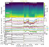 |
Fig. 1. Overview plot of the 2021 November 3 shock event. (a)–(b) Spectrograms of dynamic energy spectra measured by EPT’s sunward telescope (a) and STEP’s central 9 pixels (b). The horizontal dashed red line indicates the time interval during which proton bursts are observed. (c)–(d) Line profiles corresponding to the spectrograms in (a)–(b), respectively. STEP’s 32 energy bins and EPT’s 64 energy bins are grouped into 10 and 13 bins, respectively, with their central energies labeled on the right of the panels. (e) Temporal flux profiles of ∼268 keV protons measured by SIS’s sunward telescope (black) and ∼293 keV protons measured by EPT’s sunward telescope (pink). (f)–(h) Magnitude |B|, elevation angle θB, and azimuthal angle ϕB of the IMF. (i) Solar wind proton bulk speed |Vsw|. The IMF and solar wind speed are measured in the spacecraft frame. The dashed brown line marks the shock arrival, and the dashed yellow line marks the current sheet crossing. |
Fig. 2 shows a zoom-in plot in the vicinity of the proton bursts. After the current sheet at ∼14:15, multiple proton bursts are clearly evident at energies ranging from ∼20−30 keV to ∼1000 keV (Figs. 2a–b). The proton bursts around 14:17 also extend to lower energies of a few keV. At ∼14:23, a noticeable flux enhancement appears in a narrow energy range around ∼200 keV, similar to the monoenergetic proton event reported by Klassen et al. (2009). Moreover, most of the proton bursts last for ∼10 to 20 s, though some may last for ≲5 s or ≳50 s. None of them exhibit velocity dispersion feature. Furthermore, these transient proton bursts show distinctly different dynamic energy spectra compared to the more stable, typical downstream protons at the beginning and end of the time window shown in Fig. 2. Based on the proton dynamic energy spectra and temporal flux profiles, we selected several time intervals of clear proton bursts, labeled B1 to B5 and S1 to S2, along with two time intervals of typical downstream protons, labeled D1 and D2, to analyze their spectral features in more detail in Fig. 3. We note that the proton enhancements observed during the current sheet crossing at ∼14:15 will be investigated in a separate study.
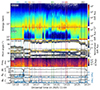 |
Fig. 2. Zoom-in plot in the vicinity of the proton bursts. (a) Dynamic energy spectrum measured by EPT’s sunward telescope. (b) Dynamic energy spectrum scaled by energy squared, measured by STEP’s central 9 pixels. This scaling enhances the prominence of higher-energy measurements (e.g., Wimmer-Schweingruber et al. 2021, 2023). (c)–(d) PAD in the solar wind frame of ∼38 keV protons measured by STEP (c) and ∼60 keV protons measured by EPT (d). The color indicates the normalized differential flux, which is normalized to the flux averaged over all available pitch angles for each time bin. Beamed distributions show higher values (yellowish) in the beaming direction and lower values (deep blue) in other directions. Isotropic distributions show values around 1 at all pitch angles. (e) Trace PSD of the magnetic field fluctuations, obtained from wavelet analysis, in units of nT2/Hz. (f)–(h) Magnitude |B|, elevation angle θB, and azimuthal angle ϕB of the IMF measured in the spacecraft frame. The blue curves in (g)–(h) show the absolute values of the variations in θB and ϕB, respectively. The vertical dashed lines bound several time intervals with labels at the top, which are analyzed in Fig. 3. |
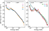 |
Fig. 3. Energy spectra averaged over the time intervals defined in Fig. 2, shown in two panels a and b for clarity. The spectra for B1 to B5 are displayed as open circles and squares, representing STEP and EPT measurements, respectively, while the spectra for S1, S2, D1, and D2 are displayed as dashed lines. The black horizontal bars at the top indicate the energy ranges covered by STEP and EPT. Other horizontal bars mark the valley and peak of the spectral bumps in corresponding colors. |
Figs. 2c–d present the PADs in the solar wind frame of ∼38 keV protons measured by STEP and ∼60 keV protons measured by EPT, respectively. Given the anti-sunward direction of the IMF after the current sheet (Fig. 2h), the proton bursts measured by STEP and EPT’s sunward telescope are traveling at pitch angles between ∼120° and ∼180°. Most of these proton bursts exhibit strong anisotropy in EPT’s proton PADs (e.g., B3 to B5 in Fig. 2d), suggesting that they are strong beams traveling anti-parallel to the IMF. Moreover, STEP’s proton PADs reveal that these proton beams have a narrow width of less than 30° (Fig. 2c). Fig. 2g shows that the IMF is pointing southward, substantially out of the ecliptic plane, during these anti-parallel traveling proton bursts. This suggests that these proton bursts could originate from a source below the ecliptic plane. One candidate source could be the part of the shock front situated below the ecliptic plane. We note that the proton bursts during B1 and B2 exhibit relatively weak anisotropy compared with other time intervals. Fig. 2e shows that the power spectral density (PSD) of 0.1−4 Hz magnetic field fluctuations exhibits no noticeable enhancements during these proton bursts compared to the background periods between them. This indicates that no apparent wave activities or enhanced turbulence levels are present during these proton bursts. In addition, these proton bursts do not coincide with significant changes in the IMF direction (blue curves in Figs. 2g–h).
Fig. 3 presents the joint energy spectra from STEP and EPT for the time intervals defined in Fig. 2. The STEP spectra transition smoothly into the EPT spectra, especially exhibiting strong agreement in the overlapping energy range covered by 3 STEP channels and 4 EPT channels. The B1 and B2 spectra show prominent bumps in the ∼20−80 keV range, with a valley at ∼20−30 keV, a peak at ∼40−50 keV, and a full width at half maximum (FWHM) of ∼30 keV (see Table 1). Both spectra exhibit a positive spectral slope between the valley and peak. In contrast, the S1 and S2 spectra are smoother, with no distinct bumps. They resemble the B1 and B2 spectra at energies above ∼50 keV but have significantly higher intensities in the ∼10−50 keV range. This suggests that the bumps in the B1 and B2 spectra arise from the low intensities of ∼10−50 keV protons, possibly caused by strong scattering during their propagation from the source to the spacecraft. We note that the proton spectrum in the solar wind frame is very similar to that in the spacecraft frame, with a slight shift in the peak energy, which is smaller than its uncertainty. We also note that the proton spectra measured by STEP exhibit similar shapes across different PAs in STEP’s FOV (not shown).
Parameters of the spectral bumps.
Fig. 3b shows that the B3 and B4 spectra exhibit prominent bumps in the ∼20−100 keV range, with parameters similar to those of the B1 and B2 spectra (see Table 1). However, they differ significantly from the D1 and D2 spectra, which represent the downstream background isotropic proton population (Gedalin et al. 2015, 2023). Furthermore, the B5 spectrum exhibits two bumps: a low-energy bump in the ∼30−100 keV range, with parameters resembling those of the B1 to B4 spectra, and a high-energy bump in the ∼100−250 keV range, peaking at ∼180 keV with an FWHM of ∼50 keV. This high-energy bump is similar to the monoenergetic proton event reported by Klassen et al. (2009).
4. Summary and discussion
We investigated the energetic proton bursts observed downstream of the 2021 November 3 shock by combining data from EPD/STEP and EPT on board Solar Orbiter. These proton bursts travel anti-parallel to the IMF in a region where the IMF is pointing southward, substantially out of the ecliptic plane. The bursts typically last for ∼10−20 s and span a wide energy range from ∼20 to ∼1000 keV. They are most prominent at energies of ∼20−100 keV in which the energy spectrum typically exhibits an evident bump. These proton bursts exhibit no velocity dispersion feature and show no correlation with significant changes in the IMF direction or with the PSD of 0.1−4 Hz magnetic field fluctuations.
The anti-parallel motion of these proton bursts along the substantially southward IMF suggests that they could originate from a source below the ecliptic plane. One candidate source could be the part of the shock front situated below the ecliptic plane. These proton bursts exhibit no velocity dispersion feature, which may suggest that these protons continuously fill the flux tubes that they are traveling in. Moreover, the intermittent occurrence of these bursts could result from the spacecraft traversing flux tubes with or without these proton beams. We find that these bursts show no correlation with significant changes in the IMF direction, indicating that their occurrence is unlikely to be caused by the local IMF changes. Instead, their intermittent occurrence could arise from the spacecraft traversing flux tubes connected to different parts of the source region with efficient or inefficient proton acceleration. The typical duration of these bursts is ∼10−20 s, corresponding to a spatial scale of ∼104 km. Variations over such small scales may suggest that these proton bursts could be accelerated by mechanisms sensitive to small-scale structures at or near the shock, such as SDA or SSA, under conditions like a varying θBn (Decker 1988) or the presence of shock front irregularities (Trotta et al. 2023a).
The B1 to B5 spectra all exhibit an evident bump in the ∼20−100 keV range. Compared with the S1 and S2 spectra, the lower intensity at energies of ∼10−50 keV and the similarity at energies above ∼50 keV suggest that the spectral bumps arise from the deficit of ∼10−50 keV protons. This deficit could result from the low-energy protons being strongly scattered en route from the source to the spacecraft due to their short mean free paths (Mason et al. 1999). Furthermore, these spectral bumps exhibit a positive spectral slope of ∼1 between the valley and the peak, which is theoretically unstable to waves or instabilities (Treumann & Baumjohann 1997). However, our observations show that no apparent wave activities or enhanced turbulence levels are present during the proton bursts. This may suggest that these proton bursts are not associated with local waves or turbulence.
The B5 spectrum exhibits an additional bump superposed in the ∼100−250 keV range with a peak at ∼180 keV. This high-energy bump is distinctly narrow, with an FWHM-to-peak ratio of 0.28 ± 0.06, in contrast to the broad low-energy bumps that typically have a ratio of ∼0.7 ± 0.2. Notably, this high-energy bump is similar to the monoenergetic proton event reported by Klassen et al. (2009, 2011), which has been attributed to acceleration mechanisms such as SDA, SSA, or acceleration by a large-scale electric field (see these references for more details). Future high-resolution simulations of particle acceleration and transport in three-dimensional shock models (e.g., Orusa & Caprioli 2023) may advance our knowledge of the acceleration and formation processes of these proton bursts.
Acknowledgments
Solar Orbiter is a mission of international cooperation between ESA and NASA, operated by ESA. EPD is supported by DLR under grant 50OT2002 and the MINCIN Project PID2019-104863RBI00/AEI/10.13039/501100011033. L.Y. is partially supported by DFG under grant HE 9270/1-1. This research at Peking University is supported in part by NSFC under contracts 42225404, 42127803, and 42150105. J.R.P. has been funded by MICIU/AEI and FEDER, UE under project PID2023-150952OB-I00/10.13039/501100011033.
References
- Bell, A. R. 1978, MNRAS, 182, 147 [Google Scholar]
- Bryant, D. A., Cline, T., Desai, U., & McDonald, F. B. 1962, J. Geophys. Res., 67, 4983 [NASA ADS] [CrossRef] [Google Scholar]
- Compton, A. H., & Getting, I. A. 1935, Phys. Rev., 47, 817 [NASA ADS] [CrossRef] [Google Scholar]
- Decker, R. B. 1988, Space Sci. Rev., 48, 195 [NASA ADS] [CrossRef] [Google Scholar]
- Dimmock, A. P., Gedalin, M., Lalti, A., et al. 2023, A&A, 679, A106 [NASA ADS] [CrossRef] [EDP Sciences] [Google Scholar]
- Dresing, N., Theesen, S., Klassen, A., & Heber, B. 2016, A&A, 588, A17 [NASA ADS] [CrossRef] [EDP Sciences] [Google Scholar]
- Fermi, E. 1954, ApJ, 119, 1 [NASA ADS] [CrossRef] [Google Scholar]
- Gedalin, M., Friedman, Y., & Balikhin, M. 2015, Phys. Plasmas, 22, 072301 [NASA ADS] [Google Scholar]
- Gedalin, M., Pogorelov, N. V., & Roytershteyn, V. 2023, ApJ, 951, 65 [CrossRef] [Google Scholar]
- Guo, X., Wang, L., Li, W., et al. 2024, ApJ, 966, L12 [Google Scholar]
- Ho, G., Lario, D., Decker, R., et al. 2003, Int. Cosmic Ray Conf., 6, 3689 [NASA ADS] [Google Scholar]
- Horbury, T., O’brien, H., Blazquez, I. C., et al. 2020, A&A, 642, A9 [NASA ADS] [CrossRef] [EDP Sciences] [Google Scholar]
- Hudson, P. D. 1965, MNRAS, 131, 23 [NASA ADS] [Google Scholar]
- Jebaraj, I., Agapitov, O., Gedalin, M., et al. 2024a, ApJ, 976, L7 [NASA ADS] [CrossRef] [Google Scholar]
- Jebaraj, I. C., Agapitov, O., Krasnoselskikh, V., et al. 2024b, ApJ, 968, L8 [NASA ADS] [CrossRef] [Google Scholar]
- Kallenrode, M.-B. 2013, Space Physics: An Introduction to Plasmas and Particles in the Heliosphere and Magnetospheres (Springer Science& Business Media) [Google Scholar]
- Kennel, C., Scarf, F., Coroniti, F., et al. 1984, J. Geophys. Res.: Space Phys., 89, 5419 [NASA ADS] [CrossRef] [Google Scholar]
- Klassen, A., Gómez-Herrero, R., Müller-Mellin, R., et al. 2009, Ann. Geophys., 27, 2077 [Google Scholar]
- Klassen, A., Gómez-Herrero, R., Müller-Mellin, R., et al. 2011, A&A, 528, A84 [NASA ADS] [CrossRef] [EDP Sciences] [Google Scholar]
- Lario, D., Ho, G., Decker, R., et al. 2003, AIP Conf. Proc., 679, 640 [NASA ADS] [CrossRef] [Google Scholar]
- Lario, D., Berger, L., Decker, R., et al. 2019, AJ, 158, 12 [NASA ADS] [CrossRef] [Google Scholar]
- Lario, D., Richardson, I., Aran, A., & Wijsen, N. 2023, ApJ, 950, 89 [NASA ADS] [CrossRef] [Google Scholar]
- Lee, M. A. 1983, J. Geophys. Res.: Space Phys., 88, 6109 [NASA ADS] [CrossRef] [Google Scholar]
- Malkov, M., & Drury, L. O. 2001, Rep. Progr. Phys., 64, 429 [Google Scholar]
- Mason, G., Von Steiger, R., Decker, R., et al. 1999, Corotating Interaction Regions: Proceedings of an ISSI Workshop 6–13 June 1998, Bern, Switzerland, Springer, 327 [Google Scholar]
- Mason, G., Ho, G., Allen, R., et al. 2023, A&A, 673, L12 [NASA ADS] [CrossRef] [EDP Sciences] [Google Scholar]
- Müller, D., Cyr, O. S., Zouganelis, I., et al. 2020, A&A, 642, A1 [NASA ADS] [CrossRef] [EDP Sciences] [Google Scholar]
- Orusa, L., & Caprioli, D. 2023, Phys. Rev. Lett., 131, 095201 [Google Scholar]
- Owen, C., Bruno, R., Livi, S., et al. 2020, A&A, 642, A16 [NASA ADS] [CrossRef] [EDP Sciences] [Google Scholar]
- Pesses, M. E., Tsurutani, B. T., Van Allen, J. A., & Smith, E. 1979, J. Geophys. Res.: Space Phys., 84, 7297 [CrossRef] [Google Scholar]
- Rodríguez-Pacheco, J., Sequeiros, J., Del Peral, L., Bronchalo, E., & Cid, C. 1998, Sol. Phys., 181, 185 [CrossRef] [Google Scholar]
- Rodríguez-Pacheco, J., Wimmer-Schweingruber, R., Mason, G., et al. 2020, A&A, 642, A7 [NASA ADS] [CrossRef] [EDP Sciences] [Google Scholar]
- Sagdeev, R. Z. 1966, Rev. Plasma Phys., 4, 23 [NASA ADS] [Google Scholar]
- Shapiro, V. D., & Üçer, D. 2003, Planet. Space Sci., 51, 665 [NASA ADS] [CrossRef] [Google Scholar]
- Treumann, R. A., & Baumjohann, W. 1997, Advanced Space Plasma Physics (London: Imperial College Press), 30 [Google Scholar]
- Trotta, D., Horbury, T. S., Lario, D., et al. 2023a, ApJ, 957, L13 [CrossRef] [Google Scholar]
- Trotta, D., Hietala, H., Horbury, T., et al. 2023b, MNRAS, 520, 437 [NASA ADS] [CrossRef] [Google Scholar]
- Tsurutani, B., & Lin, R. 1985, J. Geophys. Res.: Space Phys., 90, 1 [NASA ADS] [CrossRef] [Google Scholar]
- Vainio, R. 1999, in Plasma Turbulence and Energetic Particles in Astrophysics, eds. M. Ostrowski, & R. Schlickeiser, 232 [Google Scholar]
- Van Nes, P., Reinhard, R., Sanderson, T., Wenzel, K.-P., & Zwickl, R. 1984, J. Geophys. Res.: Space Phys., 89, 2122 [NASA ADS] [CrossRef] [Google Scholar]
- Wimmer-Schweingruber, R., Janitzek, N., Pacheco, D., et al. 2021, A&A, 656, A22 [NASA ADS] [CrossRef] [EDP Sciences] [Google Scholar]
- Wimmer-Schweingruber, R. F., Berger, L., Kollhoff, A., et al. 2023, A&A, 678, A98 [NASA ADS] [CrossRef] [EDP Sciences] [Google Scholar]
- Yang, L., Wang, L., Li, G., et al. 2018, ApJ, 853, 89 [NASA ADS] [CrossRef] [Google Scholar]
- Yang, L., Wang, L., Li, G., et al. 2019, ApJ, 875, 104 [NASA ADS] [CrossRef] [Google Scholar]
- Yang, L., Berger, L., Wimmer-Schweingruber, R. F., et al. 2020, ApJ, 888, L22 [NASA ADS] [CrossRef] [Google Scholar]
- Yang, L., Heidrich-Meisner, V., Berger, L., et al. 2023, A&A, 673, A73 [NASA ADS] [CrossRef] [EDP Sciences] [Google Scholar]
- Yang, L., Heidrich-Meisner, V., Wang, W., et al. 2024, A&A, 686, A132 [NASA ADS] [CrossRef] [EDP Sciences] [Google Scholar]
All Tables
All Figures
|
Fig. 1. Overview plot of the 2021 November 3 shock event. (a)–(b) Spectrograms of dynamic energy spectra measured by EPT’s sunward telescope (a) and STEP’s central 9 pixels (b). The horizontal dashed red line indicates the time interval during which proton bursts are observed. (c)–(d) Line profiles corresponding to the spectrograms in (a)–(b), respectively. STEP’s 32 energy bins and EPT’s 64 energy bins are grouped into 10 and 13 bins, respectively, with their central energies labeled on the right of the panels. (e) Temporal flux profiles of ∼268 keV protons measured by SIS’s sunward telescope (black) and ∼293 keV protons measured by EPT’s sunward telescope (pink). (f)–(h) Magnitude |B|, elevation angle θB, and azimuthal angle ϕB of the IMF. (i) Solar wind proton bulk speed |Vsw|. The IMF and solar wind speed are measured in the spacecraft frame. The dashed brown line marks the shock arrival, and the dashed yellow line marks the current sheet crossing. |
| In the text | |
|
Fig. 2. Zoom-in plot in the vicinity of the proton bursts. (a) Dynamic energy spectrum measured by EPT’s sunward telescope. (b) Dynamic energy spectrum scaled by energy squared, measured by STEP’s central 9 pixels. This scaling enhances the prominence of higher-energy measurements (e.g., Wimmer-Schweingruber et al. 2021, 2023). (c)–(d) PAD in the solar wind frame of ∼38 keV protons measured by STEP (c) and ∼60 keV protons measured by EPT (d). The color indicates the normalized differential flux, which is normalized to the flux averaged over all available pitch angles for each time bin. Beamed distributions show higher values (yellowish) in the beaming direction and lower values (deep blue) in other directions. Isotropic distributions show values around 1 at all pitch angles. (e) Trace PSD of the magnetic field fluctuations, obtained from wavelet analysis, in units of nT2/Hz. (f)–(h) Magnitude |B|, elevation angle θB, and azimuthal angle ϕB of the IMF measured in the spacecraft frame. The blue curves in (g)–(h) show the absolute values of the variations in θB and ϕB, respectively. The vertical dashed lines bound several time intervals with labels at the top, which are analyzed in Fig. 3. |
| In the text | |
|
Fig. 3. Energy spectra averaged over the time intervals defined in Fig. 2, shown in two panels a and b for clarity. The spectra for B1 to B5 are displayed as open circles and squares, representing STEP and EPT measurements, respectively, while the spectra for S1, S2, D1, and D2 are displayed as dashed lines. The black horizontal bars at the top indicate the energy ranges covered by STEP and EPT. Other horizontal bars mark the valley and peak of the spectral bumps in corresponding colors. |
| In the text | |
Current usage metrics show cumulative count of Article Views (full-text article views including HTML views, PDF and ePub downloads, according to the available data) and Abstracts Views on Vision4Press platform.
Data correspond to usage on the plateform after 2015. The current usage metrics is available 48-96 hours after online publication and is updated daily on week days.
Initial download of the metrics may take a while.