| Issue |
A&A
Volume 699, July 2025
|
|
|---|---|---|
| Article Number | A191 | |
| Number of page(s) | 11 | |
| Section | Galactic structure, stellar clusters and populations | |
| DOI | https://doi.org/10.1051/0004-6361/202453526 | |
| Published online | 08 July 2025 | |
Impact of ⟨3D⟩ non-local thermodynamic equilibrium on the Galactic chemical evolution of oxygen with the Radial Velocity Experiment
1
Zentrum für Astronomie der Universität Heidelberg, Landessternwarte,
Königstuhl 12,
69117
Heidelberg,
Germany
2
Max Planck Institute for Astronomy,
Königstuhl 17,
69117
Heidelberg,
Germany
3
Leibniz-Institut für Astrophysik Potsdam (AIP),
An der Sternwarte 16,
14482
Potsdam,
Germany
★ Corresponding author: guiglion@mpia.de
Received:
19
December
2024
Accepted:
19
May
2025
Context. Stellar chemical abundances, coupled with stellar kinematics, are a unique way to understand the chemo-dynamical processes that build the Milky Way (MW) and its local volume as we observe today.
Aims. However, measuring stellar abundances is challenging as one needs to properly address the effect of departure from the local thermodynamic equilibrium (LTE), as well as the commonly used 1D model atmosphere. In this work, we constrain the chemical evolution of [O/Fe] in main sequence and turn-off stars of the RAdial Velocity Experiment (RAVE) with [O/Fe] abundances derived in non-LTE (NLTE) and with horizontally temporally averaged 3D (⟨3D⟩) model atmospheres.
Methods. Using the standard spectral fitting method, we determined for the first time the LTE and NLTE abundances of oxygen from the O I triplet at 8446 Å in turn-off and dwarf stars, based on intermediate-resolution RAVE spectra and assuming both 1D and ⟨3D⟩ model atmospheres.
Resuits. We find that NLTE effects play a significant role when determining oxygen even at a resolution of R = 7500. Typical NLTE-LTE corrections of the order of −0.12 dex are measured in dwarfs and turn-off stars using 1D MARCS models. In addition, ⟨3D⟩ modelling significantly impacts the oxygen abundance measurements. In contrast to applying ⟨3D⟩ NLTE abundance corrections or the classical 1D LTE, the full ⟨3D⟩ NLTE spectral fitting improves abundance precision by nearly 10%. We also show that the decrease in [O/Fe] in the super-solar metallicity regime is characterised by a flat trend when computed in ⟨3D⟩ NLTE from a full spectral fitting. We attribute this flattening at super-solar [Fe/H] to the interplay between locally born stars with ne gative [O/Fe] and stars that migrate from the inner MW regions with super-solar [O/Fe], supporting the complex chemo-dynamical history of the Solar neighbourhood.
Conclusions. Our results are key for understanding the effects of ⟨3D⟩ and NLTE when measuring oxygen abundances in intermediate-resolution spectra. NLTE effect should be taken into account when confronting Galactic chemical evolution models with observations. This work is a test bed for the spectral analysis of the 4MOST low-resolution spectra that share similar properties as the RAVE spectra in the red wavelength domain.
Key words: methods: data analysis / techniques: spectroscopic / stars: abundances / Galaxy: stellar content
© The Authors 2025
 Open Access article, published by EDP Sciences, under the terms of the Creative Commons Attribution License (https://creativecommons.org/licenses/by/4.0), which permits unrestricted use, distribution, and reproduction in any medium, provided the original work is properly cited.
This article is published in open access under the Subscribe to Open model. Subscribe to A&A to support open access publication.
1 Introduction
Oxygen (together with other α elements such as Ne, Mg, and Ca) is mainly produced during the hydrostatic burning phases in stars with masses M> 10M⊙. The yields of massive stars are still not accurately constrained and depend mainly on the supernova model (e.g. mass loss and nuclear reaction rates; Woosley et al. 1990). The elements are diffused into the interstellar matter (ISM) via type II Supernovae (SNe) explosion. Oxygen is not processed during stellar evolution; hence, 0 abundances measured in stellar atmospheres are an accurate indicator of the enrichment of the ISM with axygen (see for instance Chiappini et al. 2003; Romano 2022). Fe-peak elements are mainly formed during explosive nucleosynthesis in type Ia SNe, on long timescales (typically 1–2 Gyr). Hence, the ratio between O and Fe abundance, namely [O/Fe]1 gives us clues on the respective contributions of type Ia and II SNe to the ISM enrichment. For instance, large [O/Fe], typically above 0, indicate that the region where the stars formed experienced a high star formation rate, and fast chemical enrichment (e.g. Matteucci & Greggio 1986). However, measuring oxygen abundances in stellar atmospheres can be a challenging task.
Largely used for computing stellar atmospheric parameters and chemical abundances in large scale surveys, the Local Thermodynamic Equilibrium (LTE) approximation remains the main pillar of spectral analysis (e.g. Nordström et al. 2004; Lee et al. 2011; Adibekyan et al. 2011; Mikolaitis et al. 2014; Guiglion et al. 2016, 2018; Stonkutė et al. 2020; Delgado Mena et al. 2021). However, the community has put strong efforts to account for departures from LTE (e.g. Mishenina et al. 2000; Mashonkina et al. 2008; Lind et al. 2011; Bergemann et al. 2013; Bergemann & Nordlander 2014a; Amarsi et al. 2020; Sitnova et al. 2021). The ultimate goal is to combine NLTE effects with a physically realistic stellar model atmosphere by transitioning from largely adopted 1D geometry and hydrostatic equilibrium to 3D hydrodynamic simulations of stellar atmospheres (e.g. Nordlander et al. 2017; Wang et al. 2024; Lind & Amarsi 2024; Storm & Bergemann 2023). NLTE and ⟨3D⟩ effects on the 6300 and 7774 Å oxygen lines are rather well known, with the 7774 Å line mainly sensitive to ⟨3D⟩ NLTE (e.g. Caffau et al. 2008; Amarsi et al. 2019; Bergemann et al. 2021). Understanding such systematics is fundamental for interpreting the chemical abundance patterns measured by large-scale spectroscopic surveys and for constraining Galactic chemical evolution models and stellar yields.
Among the large-scale spectroscopic surveys that help us understand the chemo-dynamical evolution of the Milky Way (MW), the RAdial Velocity Experiment (RAVE) made pioneering contributions in this domain (Steinmetz et al. 2006, 2020b,a, and references there-in). RAVE targeted more than half a million stars in the southern hemisphere, and the spectrograph is characterised by an intermediate spectral resolution R = λ/δλ ~ 7500, with a wavelength range centred on the Call infrared triplet (λ ∈ [8420–8780] Å). Originally designed as a spectroscopic survey for radial velocity measurements, RAVE demonstrated that significant information can be obtained from such a limited wavelength range. The RAVE consortium determined atmospheric parameters and chemical abundances of several elements, such as [α/Fe], [Mg/Fe], [Fe/H], and [Ni/Fe], using both standard spectroscopy (Boeche et al. 2011; Kordopatis et al. 2013; Steinmetz et al. 2020b) and machine–learning methods (Casey et al. 2017; Guiglion et al. 2020). With such high-quality data, numerous scientific studies have been conducted, ranging from chemo-dynamics (Boeche et al. 2014; Binney et al. 2014; Minchev et al. 2014; Kordopatis et al. 2016; Wojno et al. 2018), to the study of metal-poor stars (Matijevič et al. 2017), asteroseismology (Valentini et al. 2017), open clusters (Conrad et al. 2017), and solar twins (Jofré et al. 2017).
Although the last data release of RAVE was published in 2020, an opportunity to extract more from such a unique dataset is possible. In particular, one element remains to be measured in RAVE spectra using standard spectroscopy analysis – namely axygen (O), which can be accessed via the O I triplet lines at 8446 Å. One study, Casey et al. (2017), parametrised oxygen abundances in RAVE spectra using the machine-learning algorithm Cannon (Ness et al. 2015), based on a limited training sample (with less than 1400 stars). This study measured oxygen assuming LTE. Measuring oxygen at such a resolution with RAVE spectra is also very relevant for preparing the data analysis of the upcoming survey 4MOST (de Jong et al. 2019). Indeed, one of the main science drivers of 4MOST is to target more than 15 million stars in the Galactic disc and bulge at high- and low-resolution (4MIDABLE-HR, Bensby et al. 2019, 4MIDABLE-LR; Chiappini et al. 2019), MW halo (Helmi et al. 2019), as well as the Magellanic clouds (Cioni et al. 2019). The low-resolution optical spectrograph (λ ∈ [3700–9500] Å) has R ~ 5000–7000, i.e. very similar to RAVE in the red wavelength domain, and it covers the 01 triplet at 7774 Å. In the high-resolution spectra, O abundances in 4MOST can be derived from the [O I] line at 6300 Å. The O I line at 8446 Å has the advantage of naturally having a slightly higher resolution than the two other lines, as well as a higher signal-to-noise ratio (S/N). However, no previous study has attempted to characterise in detail the NLTE and ⟨3D⟩ effects on oxygen abundances derived with the triplet at 8446 Å. The goal of the present work is to perform the first and comprehensive ⟨3D⟩ NLTE analysis of oxygen abundances in RAVE spectra with the 8446 Å triplet.
In Section 2, we present an overview of the oxygen 8446 Å triplet region at RAVE spectral resolution. In Section 3, we measure oxygen abundance in the Sun in 1D LTE, and we show how NLTE and horizontally and temporally averaged 3D model atmospheres (⟨3D⟩) influence such a measurement. In Section 4, we present 1D/⟨3D⟩, LTE and NLTE chemical abundances of oxygen for 8018 RAVE dwarfs, while in Section 5, we perform a chemical evolution analysis of oxygen in the MW disc. We present our summary and conclusions in Section 6.
2 The behaviour of the oxygen triplet at 8446 Å
The oxygen feature at 8446 Å is composed of three strong fine-structure O I transitions at 8446.25, 8446.36, and 8446.76 Å (Kramida et al. 2024). These transitions occur between very high-excitation energy states (9.52–10.99 eV), specifically between the terms 3s 3S°−3p 3P. The total angular momenta of the upper energy states are Jupper = 0, 2, and 1, respectively, for the three transitions.
Due to the limited resolution of the RAVE spectra, we expect blends to influence our capabilities to determine oxygen abundances from such a spectral feature, especially in the cool temperature regime. To understand the contribution of the axygen lines, atomic blends, and possible presence of molecules, we generated a series of synthetic spectra in 1D LTE, 1D NLTE, and ⟨3D⟩ NLTE with typical temperature, gravity, and metallicity of stars from our RAVE sample (see Section 5): Teff = 6000 K, log(g) = 4.2, and [Fe/H] = 0.0, as well as [Fe/H] = 0.2 at solar [O/Fe]. In what follows, we provide details on the calculations of synthetic spectra with different physical models and explore the influence of blends on the analysis of stellar [O/Fe] abundance ratios.
2.1 1D LTE synthetic spectra
We used the LTE version of the Turbospectrum (Plez 2012) wrapper for the synthetic spectra generation, which is part of the spectral fitting method TSFitPy2. We adopted 1D hydrostatic MARCS model atmospheres from Gustafsson et al. (2008). The Solar abundances are taken from Magg et al. (2022). We took advantage of the atomic data from Heiter et al. (2021), which compiles high-quality atomic data for the Gaia-ESO survey. The oscillator strength of the axygen triplet lines at 8446Å are adopted from Hibbert et al. (1991), with log(gf)s = −0.463, 0.236, and 0.014, respectively. In our computation, we also included molecules from Heiter et al. (2021) that are present in the range 8440 − 8450 Å: FeH, CaH, ZrO, TiO, OH, CN, and CC.
2.2 1D NLTE synthetic spectra
It is well known that using LTE approximation can lead to large biases in measured chemical abundances (see for instance Hansen et al. 2013; Guiglion et al. 2024 for barium and strontium, Bergemann et al. 2013 for silicon, Bergemann et al. 2012a; Nordlander et al. 2017 for iron and titanium, Bergemann et al. 2019 for manganese, and Wang et al. (2024) for lithium). In the present paper, we quantify the NLTE effect on the determination of axygen abundances in RAVE spectra from the 8446 Å triplet. We generated 1D NLTE synthetic spectra using the NLTE version of Turbospectrum3,4 from Gerber et al. (2023). We adopted the O model atom of Bergemann et al. (2021), which was extensively tested on different Solar observations and was used for constraining the Solar photospheric oxygen abundance (see also Magg et al. 2022). We note that even if [Fe/H] in LTE is fed to the TSFitPy, the pipeline computes departure from NLTE for Fe.
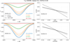 |
Fig. 1 Left row: Synthetic spectra computed at Teff = 6000 K, log(g) = 4.2, [O/Fe] = 0, in 1D LTE (dashed), 1D NTLE (dotted), and ⟨3D⟩ (solid) at RAVE resolution. The full synthesis is shown in blue, while molecules, O triplet, and Fe blend are shown in red, orange, and green, respectively. The computation was performed at [Fe/H] = +0.0 (top), and at [Fe/H] = +0.2 (bottom). Right column: Sensitivity curves of derived A(O) as a function of change in [Fe/H] of ±0.1 dex, in 1D LTE, 1D NLTE, and ⟨3D⟩, at [Fe/H] = +0.0 (top), and [Fe/H] = +0.2 (bottom). |
2.3 ⟨3D⟩ NLTE spectra
We computed ⟨3D⟩ NLTE synthetic spectra, adopting the spatially and temporarily averaged 3D model atmospheres from the STAGGER grid (Magic et al. 2013). These are full 3D radiation-hydrodynamic (RHD) simulations of the outer parts of convective envelopes of stars with F, G, and K spectral types. Their averages5 in the layers above log τ ~ 1.5 can be used as parameter-free realistic thermodynamic structures, in place of simplified 1D models in hydrostatic equilibrium, as demonstrated in a vast body of recent literature (Bergemann et al. 2012a; Osorio et al. 2015; Bergemann et al. 2017; Magg et al. 2022; Gerber et al. 2023).
Synthetic spectra are shown in Fig. 1, at the same spectral resolution as RAVE, i.e. R ~ 7500. In the left panel, we show spectra computed for a representative star in our sample (Teff = 6000 K, log(g)=4.2) at [Fe/H]= 0.0 (ξ = 1.184 km s−1), while spectra generated with [Fe/H]= +0.2 (ξ = 1.195 km s−1) are presented in the bottom left corner. We generated a series of spectra with only molecular contributions (in red), spectra with contributions only from atomic blends (Fe, in green), spectra with only the oxygen triplet (orange), and spectra with oxygen triplet plus molecules and atomic blends (blue). We observe that, independently of [Fe/H], the molecules do not contribute to the opacity. The atomic blend is mostly due to Fe I lines, especially two at 8446.385 and 8446.575 Å, with the lower-level excitation energy of 4.988 or 4.913 eV, and log(gf) of −0.920 and −1.440, respectively (Heiter et al. 2021). The strength of the Fe blend is similar in 1D LTE and ⟨3D⟩ NLTE, in both [Fe/H] regimes.
2.4 Sensitivity of A(O) to [Fe/H]
We explored how sensitive the determined A(O) abundance is to the changes in metallicity [Fe/H]. We did this by changing the input [Fe/H] by ±0.1 dex (which is typically the uncertainty in [Fe/H] for the stars in the present paper), at [Fe/H]=+0.0, and [Fe/H]=+0.2. As in the previous sections, we adopted Teff = 6000 K, log(g)=4.2, and [O/Fe]=0.0 as input parameters. We used the code TSFitPY to perform spectral fitting in a window of 3.5 Å centred on the oxygen triplet. Results are presented in the right column of Fig. 1. In 1D LTE, an uncertainty of ±0.1 dex in [Fe/H] implies a sensitivity of ±0.08 dex in A(O) at [Fe/H]=+0.0, and a sensitivity of ±0.10 dex in A(O) at [Fe/H]=+0.2 (dashed lines). Interestingly, the lowest sensitivity of A(O) to [Fe/H] is achieved in ⟨3D⟩ NLTE between 0.03 and 0.05 dex (solid line).
3 Characterising the NLTE and ⟨3D⟩ effects on Solar oxygen at RAVE resolution
3.1 1D LTE
We used the ultra-high resolution Solar atlas from Neckel (1999), which we degraded to the RAVE spectral resolution (see Fig. 2). We adopted the standard solar parameters Teff = 5777 K, log(g) = 4.44, and [Fe/H] = 0.0 (Bergemann et al. 2012b; Jofré et al. 2015). The abundance computation was performed with TSFitPY, adopting a 1D hydrostatic MARCS model atmosphere, with the linelist described in the previous section. When computing the best-fit spectrum, we naturally included a projected rotation velocity, V sin i, of 1.7km s−1 (Pavlenko et al. 2012), even hough such a contribution has a marginal effect on the quality of the fit at RAVE resolution.
To determine the Solar oxygen abundance uncertainty, we propagated uncertainties in Solar Teff, log(g), and [Fe/H], by performing a series of six spectral fits, varying the parameter one by one. We accounted for the typical uncertainties reported by Guiglion et al. (2020) for solar-like stars at RAVE spectral resolution: 70 K in Teff, 0.07 in log(g), and 0.04 in [Fe/H]. The resulting individual uncertainties when changing a given atmospheric parameter are: σ[O/Fe] = ±0.09 in Teff, σ[O/Fe] = ±0.05 in log(g), σ[O/Fe] = ±0.03 in [Fe/H]. Quadratically combining these three sources of uncertainties gives us [O/Fe]1D LTE,⊙ = −0.03 ± 0.11.
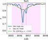 |
Fig. 2 High-resolution observation of the Sun from Neckel (1999) (blue), shown together with its version degraded to RAVE spectral resolution (orange). The best-fit spectrum, corresponding to [O/Fe] = −0.03 (1D LTE), is shown in green. The spectral fitting window is shown in light purple. |
3.2 1D NLTE
We show in Fig. 3 1D-LTE (blue, dashed) and 1D-NLTE synthetic spectra (blue, solid) at R = 7500 for [Fe/H] = [−1.0, −0.5, +0.0] and at Solar Teff, log(g), and [O/Fe]. We clearly see that NLTEs affect the 8446 Å A triplet by making the spectral feature deeper, due to the increase in opacity. It is well known that the NLTE effects in the triplet lines are mostly driven by photon losses in the lines (e.g. Bergemann & Nordlander 2014b); hence, the line source function deviates from the Planck function. We notice an increasing effect of NLTE as [Fe/H] decreases. To guide the eye, we also plotted 1D LTE spectra at ±0.2 in [O/Fe]. We see that the departure from LTE in the line strength is rather large compared to the change in LTE from [O/Fe] = 0 to [O/Fe] = +0.2. We thereby expect NLTE to play a role when determining oxygen abundances at RAVE spectral resolution. In the same fashion, as in the previous section, we measured 1D-NLTE oxygen abundances in the Solar spectrum at RAVE resolution. We used the NLTE version of TSFitPy.
Our resulting solar 1D-NLTE O abundance is [O/Fe]1D NLTE,⊙ = −0.14 ± 0.09, which is lower by 0.09 dex compared to the 1D-LTE abundance. This effect of NLTE can be directly compared to an independent estimate of the NLTE abundance correction obtained using MAFAGS-OS stellar model atmospheres and a different suite of NLTE codes (DETAIL, SIU) (Bergemann et al. 2012a, 2019). We adopted this estimate from the nlte.mpia.de database, finding a Δ (NLTE – LTE) value of −0.06 for the 8446 Å lines. We thus conclude that the NLTE correction based on MARCS+MULTI+Turbospectrum is in agreement with the estimates based on MAFAGS-OS+DETAIL+SIU. The small difference of 0.03 dex is acceptable, given the substantial differences in the physical and numerical aspects of these stellar atmospheres and spectral synthesis codes.
3.3 ⟨3D⟩ effects in LTE and NLTE
We aim here at quantifying the effects of LTE and NLTE oxygen abundances in the Sun when using ⟨3D⟩ model atmospheres. Similar to Section 3.2, we computed synthetic spectra at R = 7500 for [Fe/H] = [−1.0, −0.5, +0.0] and at Solar Teff, log(g), and [O/Fe] in ⟨3D⟩ NLTE. The spectra are plotted in orange in Fig. 3.
In LTE, oxygen features are weaker in ⟨3D⟩ (dashed orange) compared to 1D (dashed blue), independently of [Fe/H]. We observe the same behaviour in NLTE. It is consistent with the findings in Bergemann et al. (2021) and Magg et al. (2022) with the oxygen line at 777nm. Using TSFitPy to measure ⟨3D⟩ NLTE [O/Fe] in the Sun, we find [O/Fe]⟨3D⟩ NLTE,⊙ = −0.01 ± 0.09. We also computed ⟨3D⟩ LTE [O/Fe] in the Sun, and find [O/Fe]⟨3D⟩ LTE,⊙ = +0.12 ± 0.10, which is higher compared to the ⟨3D⟩ NLTE value.
4 Measuring 1D LTE, 1D NLTE, and ⟨3D⟩ NLTE oxygen abundances in RAVE stars
We adopted the flux-normalised radial-velocity corrected RAVE spectra6 from DR6 (Steinmetz et al. 2020a), used in Guiglion et al. (2020). Based on the spectral classification from RAVE DR6, we selected stars classified as normal (‘n’), for instance not suffering from any emission or binarity sign with a probability of 0.99 (see Table 4 of Steinmetz et al. 2020a; doi:10.17876/rave/dr.6/004).
Determining oxygen abundances required the atmospheric parameters Teff, log(g), as well as Fe content [Fe/H]. We adopted the machine-learning catalogue of atmospheric parameters and chemical abundances from Guiglion et al. (2020). We recall that such a machine-learning catalogue was derived using a convolutional neural-network (CNN) approach trained on high-quality stellar labels from the Apache Point Observatory Galactic Evolution Experiment, combining RAVE spectra, Gaia DR2 parallaxes, together with Two Micron All Sky Survey, Wide-field Infrared Survey Explorer, and Gaia DR2 magnitudes. The author demonstrates that such a combination of data allows us to break the spectral degeneracies inherent to the RAVE spectral range and provided improved labels compared to RAVE DR6 (see Guiglion et al. 2020 for more details). We selected the labels that are within the training set limits, i.e. the most accurate labels parametrised by CNN. We selected RAVE spectra with a S/N above 50 per pixel, for which the oxygen line was visible enough and atmospheric parameters precise enough for the chemical abundance measurement. The oxygen feature being the strongest for dwarfs (as demonstrated in Section 2), we selected RAVE stars with log(g) > 3.5 and 6300 > Teff > 5700 K, corresponding to 8018 unique RAVE stars. We notice that this RAVE sample is located within 1 kpc from the Sun.
Using TSFitPy, we derived LTE and NLTE [O/Fe] ratios in both 1D and ⟨3D⟩ for the RAVE stars following the same method as in the previous section. We adopted a fitting window defined as [8445.1–8448.4] Å. In total, we measured [O/Fe] ratios in 1D LTE, 1D NLTE, and ⟨3D⟩ NLTE for 8018 RAVE stars. We show a Kiel diagram of the RAVE stars in Fig. 4. We show examples of the line fit in Fig. 5 in the regime 50<S/N<60 per pixel. Overall, the algorithm performed very good fitting. We can judge the quality of the fit by the χ2 computed between the observation and the best-fit spectrum around the fitting window.
The fitting, χ2, increases with decreasing S/N, as shown in panel a) of Fig. 6. This is expected as the quality of the fit strongly depends on the noise present in a given RAVE spectrum (Steinmetz et al. 2020a; Guiglion et al. 2020). The overall uncertainty of [O/Fe] in ⟨3D⟩ NLTE peaks around 0.075, while 1D-LTE [O/Fe] uncertainties peak at 0.082. We can see that the main contributors to the error budgets are the uncertainties in Teff and log(g). Similar to the χ2, the uncertainty in [O/Fe] decreases with increasing S/N. However, the error budget slightly increases with decreasing temperature, due to increasing blend (panel d). The error is rather constant with log(g), while it increases with decreasing [Fe/H] due to a weaker line, as well as with super-solar [Fe/H] due to increasing blend. In Appendix A, we provide further material regarding the reliability of our RAVE [O/Fe] computed from full ⟨3D⟩ NLTE fitting.
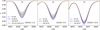 |
Fig. 3 Synthetic spectra computed with Teff = 5777 K, log(g) = 4.44, and [O/Fe] = 0.0. The LTE and NLTE spectra are indicated with dashed and solid lines, respectively. The 1D and ⟨3D⟩ computations are shown in blue and orange, respectively. Left: [Fe/H] = −1. Middle: [Fe/H] = −0.5. Right: [Fe/H] = 0.0. We also add in each panel synthetic spectra computed at [O/Fe] = ±0.2 in 1D LTE. |
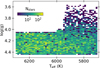 |
Fig. 4 Surface gravity vs effective temperature of the 8018 RAVE stars. |
5 Chemical evolution of oxygen with RAVE
5.1 1D LTE and NLTE [Fe/O] vs [Fe/H] diagram
In Fig. 7, we present chemical abundance trends of 1D-LTE and 1D-NLTE [O/Fe] as a function of 1D-LTE [Fe/H], binned with a step of 0.10 in [Fe/H]. Both 1D-LTE and 1D-NLTE abundances show a monotonic decrease as a function of increasing [Fe/H]. As suspected from Fig. 3, we measure lower [O/Fe] abundances in NLTE compared to LTE, by about 0.1 dex with such a shift being roughly constant with [Fe/H]. We note that the dispersion in a given [Fe/H] bin is 0.04 dex lower in 1D-NLTE compared to 1D-LTE, as NLTE tends to reduce the intrinsic dispersion.
We over-plotted a binned trend of 1D-LTE [O/Fe] from Brewer et al. (2016) with green crosses. We recall that these authors computed 1D-LTE abundances from high-resolution HIRES spectra at the Keck Observatory for a sample of ~1600 FGK exoplanet host stars (see Brewer et al. 2016 for more details). This sample is mainly confined to within 300 pc from the Sun. Our 1D-LTE [O/Fe] are in remarkable agreement with the trend from Brewer et al. (2016), which the authors derived using the oxygen triplet at 777 nm, showing a monotonic decrease in [O/Fe] with [Fe/H].
5.2 Effect of ⟨3D⟩ on [O/Fe] vs. [Fe/H] diagram
In Fig. 7, we present an average trend of ⟨3D⟩-NLTE (solid orange line) [O/Fe]. The ratio decreases with increasing [Fe/H] until solar [Fe/H], then defines a plateau in the super-solar [Fe/H] regime, contrary to 1D. Interestingly, 1D NLTE and ⟨3D⟩ NLTE are rather consistent for [Fe/H]≲−0.5. Nevertheless, the two trends largely deviate at super-solar [Fe/H].
The most interesting comparison to make in this figure is the difference in behaviour between 1D LTE and ⟨3D⟩ NLTE. While both trends decrease towards slightly super-solar [O/Fe] at solar [Fe/H], ⟨3D⟩-NLTE [O/Fe] is constant for [Fe/H] with a departure of 0.10 dex. Our ⟨3D⟩ NLTE results contradict that of Amarsi et al. (2019). Indeed, these authors find a monotonic decline of ⟨3D⟩ NLTE oxygen at super-solar [Fe/H] using the oxygen triplet at 777nm. We note that Amarsi et al. (2019) computed a full 3D-NLTE abundance correction rather than ⟨3D⟩-NLTE spectral fitting.
In the top panel of Fig. 8, we show the difference between 1D-NLTE and 1D-LTE oxygen abundances as a function of LTE [Fe/H] in RAVE stars. The mean difference is equal to −0.14 dex with a mean dispersion of 0.05. The correction is rather constant as a function of [Fe/H], but tends to converge to zero for [Fe/H] <−0.8. In the bottom panel of Fig. 8, consistent with Fig. 3, we measure an inversion in [O/Fe] ⟨3D⟩-NLTE – 1D-LTE corrections, changing from negative below solar [Fe/H] to slightly positive in the super-solar [Fe/H] regime.
The inversion is somewhat unexpected, because the ⟨3D⟩ NLTE effects in O I lines are strictly negative (see Appendix A.1) and closely match the 1D-NLTE abundance corrections. It is therefore critical to understand why we find very small, or even positive ⟨3D⟩ − 1D LTE differences for [O/Fe], when a full spectrum synthesis is used in the analysis of abundances based on the 8446 Å lines. As discussed in Sect 2.3, the effect of Fe I blends is weak in ⟨3D⟩, but more substantial in 1D LTE. In our Calculations, we aim for full internal self-consistency; that is, 1D LTE is used for O and all blends, and the same approach is adopted in 1D NLTE and ⟨3D⟩ NLTE. In the latter two cases, NLTE departure coefficients for the Fe I blends are used. We therefore closely inspected the line fits and the consistency between the best-fit synthetic profiles in 1D and ⟨3D⟩. We find that the best data-model TSFitPy solutions in ⟨3D⟩ NLTE are typically characterised by a higher macro-turbulence, compared to the fits obtained using the 1D hydrostatic model atmospheres (Fig. B.1, Appendix B). The mean macroturbulence velocity difference between the full ⟨3D⟩ NLTE spectrum synthesis and the 1D is on average 1 to 2 kms, which increases slightly with increasing [Fe/H]. Since increasing macroturbulence corresponds to shallower profiles, the abundance increases, and this effect is the origin of the systematically increasing ⟨3D⟩ NLTE [O/Fe] values obtained from the full spectrum synthesis. We emphasise that the macroturbulence values are not enforced in the calculations; rather, these values are obtained fully self-consistently with elemental abundances, which is a robust and well-established procedure (e.g. Bergemann et al. 2012a; Guiglion et al. 2024; Storm & Bergemann 2023). Not surprisingly also calculations with the average 3D models, which lack horizontal inhomogeneities, require this additional broadening component. These models only include the depth-dependent proxy of micro-turbulence, using the recipe adopted in Semenova et al. (2020, see Eq. (2)), and, thus, they do not represent the full velocity field in the 3D RHD calculations. Indeed, the large-scale velocities, in particular, are not accounted for and require additional broadening during the spectrum synthesis. We therefore consider our higher ⟨3D⟩ NLTE values of macroturbulence and abundances as more realistic and adopt them as the final best abundances in our work. We note that an in-depth analysis of velocity power spectra in 3D RHD models in the context of classical macro-scale velocities would be interesting, but it is beyond the scope of our work. Such a study was performed for red supergiants (Chiavassa et al. 2011), but a detailed investigation for Sun-like stars, as explored in this work, is warranted and encouraged.
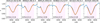 |
Fig. 5 Example of spectral fit (orange) around the oxygen triplet at 8446 Å (vertical dashed grey lines) in RAVE spectra (blue). In this figure, the RAVE spectra are characterised by 50<S/N<60. The atmospheric parameters of a given star are indicated at the top of each panel in the form Teff/log(g)/[Fe/H]. The fitting window is indicated in light purple. |
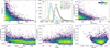 |
Fig. 6 (a) χ2 between the RAVE observation and the best-fit spectrum in ⟨3D⟩ NLTE around the oxygen triplet at 8446 Å, provided by TSFitPy, as a function of S/N for 8018 RAVE stars. (b) ⟨3D⟩ NLTE [O/Fe] uncertainty distribution (solid black line). We also show the individual distributions of ⟨3D⟩-NLTE uncertainties due to uncertainties in Teff (blue), log(g) (orange), and [Fe/H] (green). For comparison, we show the [O/Fe] uncertainty distribution in 1D LTE (dashed black line). (c) ⟨3D⟩ NLTE [O/Fe] uncertainties vs. S/N. (d–f) The ⟨3D⟩-NLTE [O/Fe] uncertainties as a function of Teff, log(g), and [Fe/H], respectively. |
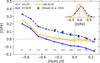 |
Fig. 7 Average [O/Fe] abundances as a function of LTE [Fe/H] for 8018 RAVE stars. The blue dots show 1D-LTE abundances (dashed blue line) and 1D-NLTE abundances (solid blue line). The orange crosses show ⟨3D⟩ LTE abundances (dashed orange line) and ⟨3D⟩ NLTE (solid orange line). We also show a kernel density distribution of the 1D-LTE and ⟨3D⟩-NLTE [O/Fe] abundances in the top-right corner. An average trend computed using the 1D-LTE data for stars in the solar neighbourhood from Brewer et al. (2016) is shown in green crosses. |
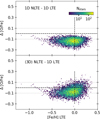 |
Fig. 8 2D histogram of the difference in [O/Fe] abundances: 1D NLTE – 1D LTE (left), ⟨3D⟩ NLTE – ⟨3D⟩ LTE (middle), and ⟨3D⟩ NLE – 1D LTE, as a function of LTE [Fe/H]. |
5.3 Impact of ⟨3D⟩ NLTE of our understanding of the [O/Fe] vs. [Fe/H] diagram
We ask how the inversion in ⟨3D⟩-NLTE – 1D-LTE [O/Fe] impacts our understanding of the chemical evolution of [O/Fe] with [Fe/H], especially in the super-solar [Fe/H] regime. The shallow monotonic decline of [O/Fe] versus [Fe/H] observed in MW stars supports a scenario of a chemical evolution in the disc where both SN Ia and SN II contribute at a steady rate to the enrichment of the interstellar medium. As a result, it produces a decline in [O/Fe] with [Fe/H] (see for instance Chiappini et al. 2003). Our 1D-LTE [O/Fe] declines with [Fe/H], while our ⟨3D⟩ NLTE [O/Fe] levels out for [Fe/H]>0. For [Fe/H]>, we propose that the flattening of [O/Fe] could be a sign of the presence of multiple stellar populations in the Solar neighbourhood.
Indeed, it is now well accepted in the literature that the Solar neighbourhood (within ~2 kpc of the Sun) is populated by locally born stars and stars born in the inner regions of the MW (see for instance Casagrande et al. 2011; Trevisan et al. 2011; Guiglion et al. 2019). It was proposed that a significant proportion of the stars born in the inner regions migrated towards the outer regions of the MW disc due to radial migration (e.g. Roškar et al. 2008; Schönrich & Binney 2009; Vera-Ciro et al. 2014). The amplitude of such a migration depends on the birth radius of the star itself and the age of the star (see Figure 3 of Minchev et al. 2013). In order to migrate from the inner-regions to the solar neighbourhood, metal rich stars must be old (4–8 Gyr). We checked the stellar age7 distribution of the RAVE stars with [Fe/H] >0 used here and obtained the following result: 87% of the sample is confined between 2 and 8 Gyr, with a median value of ~5Gyr. The stars observed in the super-metallicity regime are not only young, but also cover a wide range of stellar ages. This is consistent with previous findings (e.g. Anders et al. 2017; Dantas et al. 2022, 2023). Recent estimates of stellar birth radii confirmed that a large fraction of super metal-rich stars come from the inner regions of the disc (see Figure 8 of Minchev et al. 2018).
Galactic chemical evolution models (e.g. Matteucci & Brocato 1990; Chiappini et al. 2001; Minchev et al. 2013) and observations of very metal-rich stars in the Galactic bulge (e.g. Nepal et al. 2023; Feldmeier-Krause 2022; Rix et al. 2024) support the scenario that the inner regions of the MW underwent early (~107 yr) rapid star formation. The star formation rate has been more efficient than in the solar vicinity by a factor of 10 (Matteucci & Brocato 1990) (in contrast to the outer disc, where slow and late star formation yield subsolar [Fe/H] in the outer MW regions; e.g. Bergemann et al. 2014). In the super-solar metallicity regime, stars originating from the inner MW regions (i.e. the bulge) are expected to be super-solar abundant in [α/Fe], including oxygen (see for instance Figure 4 of Matteucci & Brocato 1990). Hence, we propose that the flattening of [O/Fe] at super-solar [Fe/H] observed in our RAVE data can be interpreted as a mix of stellar populations: one locally born exhibiting subsolar [O/Fe] consistently with a pure decline scenario, and another characterised by high values of [O/Fe], due to high star formation efficiency within inner regions of the MW8.
6 Conclusion
In this paper, we focused on constraining the chemical evolution of oxygen in ⟨3D⟩ NLTE for the first time with spectra from RAVE. We summarise here our methodology and main findings:
Using the standard spectral fitting code TSFitPy Gerber et al. 2023; Storm & Bergemann 2023, we performed a careful abundance analysis of the Solar spectrum at RAVE resolution (Sect. 3, Fig. 2, Fig. 3) deriving 1D LTE, 1D NLTE, and ⟨3D⟩ NLTE [O/Fe] based on the oxygen triplet at 8446 Å. We find [O/Fe]1D LTE,⊙ = −0.03 ± 0.11, and [O/Fe]⟨3D⟩ NLTE,⊙ = −0.01 ± 0.09.
We selected 8018 main-sequence and turn-off stars from the RAVE survey with high-quality atmospheric parameters from Guiglion et al. (2020), covering −1 <[Fe/H]< +0.4 (see Sect. 4). With TSFitPy, we performed high-quality measurements of [O/Fe] in RAVE spectra (R ~ 7500; see Fig. 5, Fig. 6).
Table 1[O/Fe] ratios and uncertainties of the publicly available online catalogue of 8818 RAVE turn-off and dwarf stars.
We show that the difference between 1D-NLTE and 1D-LTE [O/Fe] is constant with [Fe/H] in RAVE stars, with a mean difference of −0.14 dex (Fig. 8). Similar results are obtained when comparing ⟨3D⟩-NLTE [O/Fe] to 1D-LTE [O/Fe]. When comparing ⟨3D⟩-NLTE [O/Fe] to 1D-LTE [O/Fe], the difference is negative below [Fe/H]=0, while it becomes positive for super-solar [Fe/H].
The 1D-LTE abundance pattern of [O/Fe] versus [Fe/H] in RAVE stars shows a monotonic decrease with increasing [Fe/H]. Such a trend matches the 1D LTE abundance trend of the very local (d<300pc) exoplanet host stars of Brewer et al. (2016) very well based on high-resolution spectra (Fig. 7). The [O/Fe] in ⟨3D⟩ NLTE decreases with [Fe/H] until [Fe/H]=0, and then flattens for [Fe/H]>0, contrary to the trend seen in 1D LTE as commonly measured in the literature. This result is found only when performing a full spectral analysis, as opposed to applying ⟨3D⟩ NLTE corrections.
We propose that the flattening of [O/Fe] for [Fe/H]>0 is due to the interplay between locally born stars (showing negative [O/Fe]) and stars, which migrated from inner MW regions characterised by rapid early star formation and super-solar [O/Fe].
This work shows that at intermediate resolutions, significant information can be extracted from the oxygen triplet at 8446 Å. This feature will be present in low-resolution 4MOST spectra (R ~ 7000 at 8500 Å), providing good insight into oxygen derivation in the 4MOST FORMIDABLE-LR survey. In addition, the 4MOST low-resolution spectrograph will cover the oxygen forbidden line at 6300 Å, as well as the oxygen triplet at 7774 Å. The 4MOST high-resolution setup (R ~ 22 500) will also cover the forbidden line at 6300 Å, allowing us to determine useful abundances. This study demonstrates that that NLTE effects and the realistic treatment of convection using average 3D models are key for accurate abundance diagnostics even when low- and intermediate-resolution spectra are used. Future low-resolution surveys such as 4MOST and WEAVE will need to properly include such effects in their analysis pipeline.
Data availability
The catalogue of 1D LTE, ⟨3D⟩ NLTE [O/Fe], uncertainties and χ2 between the best fit spectrum and RAVE observation is available on the RAVE database at doi.org/10.17876/rave/dr.6/101. The catalogue is summarised in Table 1.
Acknowledgements
G.G. acknowledges the anonymous referee for the comments and suggestions that improved the readability of the paper. G.G. sincerely thanks M. Bergemann, N. Storm, and M. Steinmetz for the fruitful discussions, as well as Š. Mikolaitis for kindly sharing VUES spectra. G.G. acknowledges support by Deutsche Forschungs-gemeinschaft (DFG, German Research Foundation) – project-IDs: eBer-22-59652 (GU 2240/1-1 “Galactic Archaeology with Convolutional Neural-Networks: Realising the potential of Gaia and 4MOST”). This project has received funding from the European Research Council (ERC) under the European Union’s Horizon 2020 research and innovation programme (Grant agreement No. 949173). This work has been partially done in the frame of the Trans-National access programme of Europlanet 2024 RI which has received funding from the European Union’s Horizon 2020 research and innovation programme under grant agreement No. 871149 project number 20-EPN2-081. This work made use of public data from the RAVE survey (https://www.rave-survey.org). This work made use of overleaf9, and of the following PYTHON packages (not previously mentioned): MATPLOTLIB (Hunter 2007), NUMPY (Harris et al. 2020), PANDAS (McKinney 2010), SEABORN (Waskom 2021).
Appendix A Are full ⟨3D⟩-NLTE [O/Fe] ratios more precise than 1D-LTE [O/Fe] corrected from ⟨3D⟩-NLTE effects?
As detailed in the introduction, several past studies derived 1D NLTE (or ⟨3D⟩ NLTE) abundances from 1D LTE and applied NLTE (or ⟨3D⟩ NLTE) corrections. Throughout the paper, we derived [O/Fe] ratios from full ⟨3D⟩ NLTE analysis of RAVE spectra. As an extra validation, we computed ⟨3D⟩ NLTE corrections based on the routine calculate_nlte_correction_line.py from TSFitPy. This routine takes as input the atmospheric parameters of a given star, and well as its 1D-LTE [O/Fe], and calculates pure ⟨3D⟩ NLTE correction without fitting the spectrum. We note that when using abundance corrections, only oxygen abundance is being corrected.
A.1 Comparison between full ⟨3D⟩ NLTE and corrected ⟨3D⟩ NLTE [O/Fe]
Fig. A.1 shows a similar figure as Fig. 7, but we overploted ⟨3D⟩ NLTE binned [O/Fe] computed from theoretical ⟨3D⟩ NLTE corrections. One can see that the corrected ⟨3D⟩ NLTE [O/Fe] ratio (in red) monotonically decreases with increasing [Fe/H], similarly to the 1D LTE and 1D NLTE curves. In the top right corner, the corrected ⟨3D⟩ NLTE [O/Fe] distribution (red) is broader (σ = 0.26) than the 1D LTE (σ = 0.22), and the ⟨3D⟩ NLTE [O/Fe] distribution (in orange, σ = 0.18). It suggests that the most precise method to derive ⟨3D⟩ NLTE [O/Fe] is by applying full ⟨3D⟩ NLTE spectral fitting, as performed throughout this paper on RAVE data.
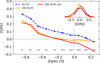 |
Fig. A.1 Same Figure as Fig. 7, together with [O/Fe] computed in RAVE from ⟨3D⟩ NLTE corrections (in red). |
A.2 [O/Fe] trend with log(g) and Teff
Fig. A.2 presents binned [O/Fe] ratios as a functions of log(g) (top) and Teff (bottom). Both [O/Fe] ratios computed in 1D LTE (blue, dashed) and corrected from ⟨3D⟩ NLTE (red, solid) present strong trends with gravity and temperature. [O/Fe] computed with full ⟨3D⟩ NLTE fitting presents a weak trend with log(g) while is constant with temperature, showing a very good accuracy with log(g) and Teff. Several studies already reported that NLTE abundances computed from corrections may lead to systematics (see for instance Kirby et al. 2018).
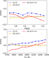 |
Fig. A.2 [O/Fe] ratios computed in RAVE as a function of log(g) (top) and Teff (bottom). |
A.3 Systematic comparison between [O/Fe] derived with O triplets at 777 and 844nm
In the present paper, we derived for the first time [O/Fe] ratios in ⟨3D⟩ NLTE with the O triplet at 844nm. We aim here at measuring the systematic difference between [O/Fe] computed with the triplets at 777 and 844 nm. Both the 777 nm and the 844nm lines arise from energy states with similar lower excitation potentials of approx. 9.14 eV (777 nm) and 9.52 eV (844 nm), and the upper energy states are also similar (10.74 vs 10.99 eV). In addition, we characterise this difference by using both full ⟨3D⟩ NLTE fitting and ⟨3D⟩ NLTE corrected.
To do so, we adopted a sample of 60 FG dwarfs observed by the high resolution VUES instrument covering the same atmospheric parameter range as our RAVE sample (Š. Mikolaitis, private communication). Such spectra cover the whole optical + near infrared domain, and have been extensively used for chemical abundance diagnostics (see Stonkutė et al. 2020; Tautvaišienė et al. 2021; Sharma et al. 2024 for details on the instrument and science applications). The VUES spectra were degraded to RAVE resolution, and we used the 1D LTE atmospheric parameters from Tautvaišienė et al. (2020); Mikolaitis et al. (2019). We performed spectral fitting following the same strategy as in Section 4 of the present paper. We also computed ⟨3D⟩ NLTE corrections as in Section A. We note that the detailed analysis of the full VUES dataset will be presented in a subsequent publication (Guiglion et al. in prep.).
In Fig. A.3, we presented density distributions of the differences between [O/Fe] ratios computed with the 777nm and 844nm O triplets. The orange line, based on [O/Fe] computed with full ⟨3D⟩ NLTE fitting is characterised by a mean difference ⟨Δ⟩ = +0.04 dex and a dispersion σ = 0.16. The red line, based on [O/Fe] computed with ⟨3D⟩ NLTE corrections is characterised by ⟨Δ⟩ = +0.12 dex, and σ = 0.22 dex. Here again, in the case of VUES spectra, it is clear that the full ⟨3D⟩ NLTE fitting is more precise and accurate than applying ⟨3D⟩ NLTE corrections to 1D-LTE [O/Fe] ratios.
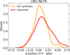 |
Fig. A.3 Density distribution of the differences between [O/Fe] computed with the 777nm and 844nm triplets in the VUES spectra. The orange curve corresponds to [O/Fe] ratios computed with a full ⟨3D⟩ NLTE fitting, while the red line corresponds to [O/Fe] computed from ⟨3D⟩ NLTE corrections. |
Appendix B On macroturbulence velocities
In Fig. B.1, we present macroturbulence velocity differences between ⟨3D⟩ NLTE and 1D LTE, as a function of input Teff, log(g), and [Fe/H]. On average this difference is about 1.7 km s−1. While this difference is constant as a function of Teff and log(g), it increases from 1 km s−1 at [Fe/H]~-0.5 to 1.7 km s−1 at [Fe/H]~0.0, and 1.9 km s−1 at [Fe/H]~+0.1.
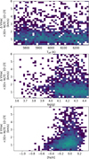 |
Fig. B.1 Difference in macro-turbulence velocities obtained during the spectral fitting between ⟨3D⟩ NLTE and 1D LTE, as a function of Teff, log(g), and [Fe/H] in RAVE stars. |
References
- Adibekyan, V. Z., Santos, N. C., Sousa, S. G., & Israelian, G. 2011, A&A, 535, L11 [NASA ADS] [CrossRef] [EDP Sciences] [Google Scholar]
- Amarsi, A. M., Nissen, P. E., & Skúladóttir, Á. 2019, A&A, 630, A104 [NASA ADS] [CrossRef] [EDP Sciences] [Google Scholar]
- Amarsi, A. M., Lind, K., Osorio, Y., et al. 2020, A&A, 642, A62 [EDP Sciences] [Google Scholar]
- Anders, F., Chiappini, C., Minchev, I., et al. 2017, A&A, 600, A70 [NASA ADS] [CrossRef] [EDP Sciences] [Google Scholar]
- Bensby, T., Bergemann, M., Rybizki, J., et al. 2019, The Messenger, 175, 35 [NASA ADS] [Google Scholar]
- Bergemann, M., & Nordlander, T. 2014a, in Determination of Atmospheric Parameters of B, eds. E. Niemczura, B. Smalley, & W. Pych, 169 [CrossRef] [Google Scholar]
- Bergemann, M., & Nordlander, T. 2014b, in Determination of Atmospheric Parameters of B, 169 [CrossRef] [Google Scholar]
- Bergemann, M., Kudritzki, R.-P., Plez, B., et al. 2012a, ApJ, 751, 156 [Google Scholar]
- Bergemann, M., Lind, K., Collet, R., Magic, Z., & Asplund, M. 2012b, MNRAS, 427, 27 [Google Scholar]
- Bergemann, M., Kudritzki, R.-P., Würl, M., et al. 2013, ApJ, 764, 115 [NASA ADS] [CrossRef] [Google Scholar]
- Bergemann, M., Ruchti, G. R., Serenelli, A., et al. 2014, A&A, 565, A89 [NASA ADS] [CrossRef] [EDP Sciences] [Google Scholar]
- Bergemann, M., Collet, R., Schönrich, R., et al. 2017, ApJ, 847, 16 [Google Scholar]
- Bergemann, M., Gallagher, A. J., Eitner, P., et al. 2019, A&A, 631, A80 [NASA ADS] [CrossRef] [EDP Sciences] [Google Scholar]
- Bergemann, M., Hoppe, R., Semenova, E., et al. 2021, MNRAS, 508, 2236 [NASA ADS] [CrossRef] [Google Scholar]
- Binney, J., Burnett, B., Kordopatis, G., et al. 2014, MNRAS, 439, 1231 [NASA ADS] [CrossRef] [Google Scholar]
- Boeche, C., Siebert, A., Williams, M., et al. 2011, AJ, 142, 193 [NASA ADS] [CrossRef] [Google Scholar]
- Boeche, C., Siebert, A., Piffl, T., et al. 2014, A&A, 568, A71 [NASA ADS] [CrossRef] [EDP Sciences] [Google Scholar]
- Brewer, J. M., Fischer, D. A., Valenti, J. A., & Piskunov, N. 2016, ApJS, 225, 32 [Google Scholar]
- Caffau, E., Ludwig, H. G., Steffen, M., et al. 2008, A&A, 488, 1031 [CrossRef] [EDP Sciences] [Google Scholar]
- Casagrande, L., Schönrich, R., Asplund, M., et al. 2011, A&A, 530, A138 [NASA ADS] [CrossRef] [EDP Sciences] [Google Scholar]
- Casey, A. R., Hawkins, K., Hogg, D. W., et al. 2017, ApJ, 840, 59 [NASA ADS] [CrossRef] [Google Scholar]
- Chiappini, C., Matteucci, F., & Romano, D. 2001, ApJ, 554, 1044 [NASA ADS] [CrossRef] [Google Scholar]
- Chiappini, C., Romano, D., & Matteucci, F. 2003, MNRAS, 339, 63 [NASA ADS] [CrossRef] [Google Scholar]
- Chiappini, C., Minchev, I., Starkenburg, E., et al. 2019, The Messenger, 175, 30 [NASA ADS] [Google Scholar]
- Chiavassa, A., Freytag, B., Masseron, T., & Plez, B. 2011, A&A, 535, A22 [NASA ADS] [CrossRef] [EDP Sciences] [Google Scholar]
- Cioni, M.. R. L., Storm, J., Bell, C. P. M., et al. 2019, The Messenger, 175, 54 [NASA ADS] [Google Scholar]
- Conrad, C., Scholz, R. D., Kharchenko, N. V., et al. 2017, A&A, 600, A106 [NASA ADS] [CrossRef] [EDP Sciences] [Google Scholar]
- Dantas, M. L. L., Guiglion, G., Smiljanic, R., et al. 2022, A&A, 668, L7 [NASA ADS] [CrossRef] [EDP Sciences] [Google Scholar]
- Dantas, M. L. L., Smiljanic, R., Boesso, R., et al. 2023, A&A, 669, A96 [NASA ADS] [CrossRef] [EDP Sciences] [Google Scholar]
- de Jong, R. S., Agertz, O., Berbel, A. A., et al. 2019, The Messenger, 175, 3 [NASA ADS] [Google Scholar]
- Delgado Mena, E., Adibekyan, V., Santos, N. C., et al. 2021, A&A, 655, A99 [NASA ADS] [CrossRef] [EDP Sciences] [Google Scholar]
- Feldmeier-Krause, A. 2022, MNRAS, 513, 5920 [Google Scholar]
- Gerber, J. M., Magg, E., Plez, B., et al. 2023, A&A, 669, A43 [NASA ADS] [CrossRef] [EDP Sciences] [Google Scholar]
- Guiglion, G., de Laverny, P., Recio-Blanco, A., et al. 2016, A&A, 595, A18 [NASA ADS] [CrossRef] [EDP Sciences] [Google Scholar]
- Guiglion, G., de Laverny, P., Recio-Blanco, A., & Prantzos, N. 2018, A&A, 619, A143 [NASA ADS] [CrossRef] [EDP Sciences] [Google Scholar]
- Guiglion, G., Chiappini, C., Romano, D., et al. 2019, A&A, 623, A99 [NASA ADS] [CrossRef] [EDP Sciences] [Google Scholar]
- Guiglion, G., Matijevič, G., Queiroz, A. B. A., et al. 2020, A&A, 644, A168 [EDP Sciences] [Google Scholar]
- Guiglion, G., Bergemann, M., Storm, N., et al. 2024, A&A, 683, A73 [NASA ADS] [CrossRef] [EDP Sciences] [Google Scholar]
- Gustafsson, B., Edvardsson, B., Eriksson, K., et al. 2008, A&A, 486, 951 [NASA ADS] [CrossRef] [EDP Sciences] [Google Scholar]
- Hansen, C. J., Bergemann, M., Cescutti, G., et al. 2013, A&A, 551, A57 [NASA ADS] [CrossRef] [EDP Sciences] [Google Scholar]
- Harris, C. R., Millman, K. J., van der Walt, S. J., et al. 2020, Nature, 585, 357 [NASA ADS] [CrossRef] [Google Scholar]
- Heiter, U., Lind, K., Bergemann, M., et al. 2021, A&A, 645, A106 [EDP Sciences] [Google Scholar]
- Helmi, A., Irwin, M., Deason, A., et al. 2019, The Messenger, 175, 23 [NASA ADS] [Google Scholar]
- Hibbert, A., Biemont, E., Godefroid, M., & Vaeck, N. 1991, J. Phys. B At. Mol. Phys., 24, 3943 [NASA ADS] [CrossRef] [Google Scholar]
- Hunter, J. D. 2007, Comput. Sci. Eng., 9, 90 [NASA ADS] [CrossRef] [Google Scholar]
- Jofré, P., Heiter, U., Soubiran, C., et al. 2015, A&A, 582, A81 [Google Scholar]
- Jofré, P., Traven, G., Hawkins, K., et al. 2017, MNRAS, 472, 2517 [Google Scholar]
- Kirby, E. N., Xie, J. L., Guo, R., Kovalev, M., & Bergemann, M. 2018, ApJS, 237, 18 [NASA ADS] [CrossRef] [Google Scholar]
- Kordopatis, G., Gilmore, G., Steinmetz, M., et al. 2013, AJ, 146, 134 [Google Scholar]
- Kordopatis, G., Wyse, R. F. G., & Binney, J. 2016, Astron. Nachr., 337, 904 [Google Scholar]
- Kramida, A., Yu. Ralchenko, Reader, J., & and NIST ASD Team 2024, NIST Atomic Spectra Database (ver. 5.12), [Online]. Available: https://physics.nist.gov/asd [2025, April 3], National Institute of Standards and Technology, Gaithersburg, MD [Google Scholar]
- Lee, Y. S., Beers, T. C., An, D., et al. 2011, ApJ, 738, 187 [NASA ADS] [CrossRef] [Google Scholar]
- Lind, K., & Amarsi, A. M. 2024, ARA&A, 62, 475 [NASA ADS] [CrossRef] [Google Scholar]
- Lind, K., Asplund, M., Barklem, P. S., & Belyaev, A. K. 2011, A&A, 528, A103 [NASA ADS] [CrossRef] [EDP Sciences] [Google Scholar]
- Magg, E., Bergemann, M., Serenelli, A., et al. 2022, A&A, 661, A140 [NASA ADS] [CrossRef] [EDP Sciences] [Google Scholar]
- Magic, Z., Collet, R., Asplund, M., et al. 2013, A&A, 557, A26 [NASA ADS] [CrossRef] [EDP Sciences] [Google Scholar]
- Mashonkina, L., Zhao, G., Gehren, T., et al. 2008, A&A, 478, 529 [NASA ADS] [CrossRef] [EDP Sciences] [Google Scholar]
- Matijevič, G., Chiappini, C., Grebel, E. K., et al. 2017, A&A, 603, A19 [NASA ADS] [CrossRef] [EDP Sciences] [Google Scholar]
- Matteucci, F., & Greggio, L. 1986, A&A, 154, 279 [NASA ADS] [Google Scholar]
- Matteucci, F., & Brocato, E. 1990, ApJ, 365, 539 [CrossRef] [Google Scholar]
- McKinney, W. 2010, in Proceedings of the 9th Python in Science Conference, eds. S. van der Walt, & J. Millman, 56 [Google Scholar]
- McMillan, P. J., Kordopatis, G., Kunder, A., et al. 2018, MNRAS, 477, 5279 [NASA ADS] [CrossRef] [Google Scholar]
- Mikolaitis, Š., Hill, V., Recio-Blanco, A., et al. 2014, A&A, 572, A33 [NASA ADS] [CrossRef] [EDP Sciences] [Google Scholar]
- Mikolaitis, Š., Drazdauskas, A., Minkevičiūtė, R., et al. 2019, A&A, 628, A49 [EDP Sciences] [Google Scholar]
- Minchev, I., Chiappini, C., & Martig, M. 2013, A&A, 558, A9 [CrossRef] [EDP Sciences] [Google Scholar]
- Minchev, I., Chiappini, C., Martig, M., et al. 2014, ApJ, 781, L20 [Google Scholar]
- Minchev, I., Anders, F., Recio-Blanco, A., et al. 2018, MNRAS, 481, 1645 [NASA ADS] [CrossRef] [Google Scholar]
- Mishenina, T. V., Korotin, S. A., Klochkova, V. G., & Panchuk, V. E. 2000, A&A, 353, 978 [NASA ADS] [Google Scholar]
- Neckel, H. 1999, Sol. Phys., 184, 421 [Google Scholar]
- Nepal, S., Guiglion, G., de Jong, R. S., et al. 2023, A&A, 671, A61 [NASA ADS] [CrossRef] [EDP Sciences] [Google Scholar]
- Ness, M., Hogg, D. W., Rix, H. W., Ho, A. Y. Q., & Zasowski, G. 2015, ApJ, 808, 16 [NASA ADS] [CrossRef] [Google Scholar]
- Nordlander, T., Amarsi, A. M., Lind, K., et al. 2017, A&A, 597, A6 [NASA ADS] [CrossRef] [EDP Sciences] [Google Scholar]
- Nordström, B., Mayor, M., Andersen, J., et al. 2004, A&A, 418, 989 [Google Scholar]
- Osorio, Y., Barklem, P. S., Lind, K., et al. 2015, A&A, 579, A53 [NASA ADS] [CrossRef] [EDP Sciences] [Google Scholar]
- Pavlenko, Y. V., Jenkins, J. S., Jones, H. R. A., Ivanyuk, O., & Pinfield, D. J. 2012, MNRAS, 422, 542 [NASA ADS] [CrossRef] [Google Scholar]
- Plez, B. 2012, Turbospectrum: Code for spectral synthesis, Astrophysics Source Code Library [record ascl:1205.004] [Google Scholar]
- Rix, H.-W., Chandra, V., Zasowski, G., et al. 2024, ApJ, 975, 293 [NASA ADS] [CrossRef] [Google Scholar]
- Romano, D. 2022, A&A Rev., 30, 7 [NASA ADS] [CrossRef] [Google Scholar]
- Roškar, R., Debattista, V. P., Quinn, T. R., Stinson, G. S., & Wadsley, J. 2008, ApJ, 684, L79 [Google Scholar]
- Schönrich, R., & Binney, J. 2009, MNRAS, 396, 203 [Google Scholar]
- Semenova, E., Bergemann, M., Deal, M., et al. 2020, A&A, 643, A164 [NASA ADS] [CrossRef] [EDP Sciences] [Google Scholar]
- Sharma, A., Stonkutė, E., Drazdauska, A., et al. 2024, A&A, 691, A160 [NASA ADS] [CrossRef] [EDP Sciences] [Google Scholar]
- Sitnova, T. M., Mashonkina, L. I., Tatarnikov, A. M., et al. 2021, MNRAS, 504, 1183 [NASA ADS] [CrossRef] [Google Scholar]
- Steinmetz, M., Zwitter, T., Siebert, A., et al. 2006, AJ, 132, 1645 [Google Scholar]
- Steinmetz, M., Guiglion, G., McMillan, P. J., et al. 2020a, AJ, 160, 83 [NASA ADS] [CrossRef] [Google Scholar]
- Steinmetz, M., Matijevič, G., Enke, H., et al. 2020b, AJ, 160, 82 [NASA ADS] [CrossRef] [Google Scholar]
- Stonkutė, E., Chorniy, Y., Tautvaišienė, G., et al. 2020, AJ, 159, 90 [Google Scholar]
- Storm, N., & Bergemann, M. 2023, MNRAS, 525, 3718 [NASA ADS] [CrossRef] [Google Scholar]
- Tautvaišienė, G., Mikolaitis, S., Drazdauskas, A., et al. 2020, ApJS, 248, 19 [NASA ADS] [CrossRef] [Google Scholar]
- Tautvaišienė, G., Viscasillas Vázquez, C., Mikolaitis, Š., et al. 2021, A&A, 649, A126 [NASA ADS] [CrossRef] [EDP Sciences] [Google Scholar]
- Trevisan, M., Barbuy, B., Eriksson, K., et al. 2011, A&A, 535, A42 [NASA ADS] [CrossRef] [EDP Sciences] [Google Scholar]
- Valentini, M., Chiappini, C., Davies, G. R., et al. 2017, A&A, 600, A66 [NASA ADS] [CrossRef] [EDP Sciences] [Google Scholar]
- Vera-Ciro, C., D’Onghia, E., Navarro, J., & Abadi, M. 2014, ApJ, 794, 173 [NASA ADS] [CrossRef] [Google Scholar]
- Wang, E. X., Nordlander, T., Buder, S., et al. 2024, MNRAS, 528, 5394 [CrossRef] [Google Scholar]
- Waskom, M. L. 2021, J. Open Source Softw., 6, 3021 [CrossRef] [Google Scholar]
- Wojno, J., Kordopatis, G., Steinmetz, M., et al. 2018, MNRAS, 477, 5612 [Google Scholar]
- Woosley, S. E., Hartmann, D. H., Hoffman, R. D., & Haxton, W. C. 1990, ApJ, 356, 272 [NASA ADS] [CrossRef] [Google Scholar]
![$\[[\mathrm{O} / \mathrm{Fe}]{=}\log \left[\frac{\mathrm{N}(\mathrm{O})}{\mathrm{N}(\mathrm{Fe})}\right]_{\star}-\log \left[\frac{\mathrm{N}(\mathrm{O})}{\mathrm{N}(\mathrm{Fe})}\right]_{\odot}.\]$](/articles/aa/full_html/2025/07/aa53526-24/aa53526-24-eq1.png)
We note that the NLTE version of Turbospectrum uses grids of NLTE departure coefficients to compute NLTE profiles of lines. This is done by correcting the opacity and the source functions of all lines. These correction grids were computed for 1D MARCS and averaged 3D model atmospheres and were publicly released as a part of the original paper on Turbospectrum NLTE v. 20 (see Gerber et al. 2023 for mote details).
The RAVE spectra are available at doi:10.17876/rave/dr.6/019, together with the RAVE radial velocities at doi:10.17876/rave/dr.6/001
We adopted the stellar ages from RAVE DR6 (Steinmetz et al. 2020a) derived by the BDASP pipeline (Table 9; doi:10.17876/rave/dr.6/008), which is a Bayesian framework demonstrated in McMillan et al. (2018).
This scenario aligns very well with Guiglion et al. (2019) who suggested that the decrease of the lithium envelope at [Fe/H] of Solar neighbourhood stars was the result of mixed stellar population: locally born stars with depleted lithium, together with radially migrated stars from the inner-regions with high-lithium content.
All Tables
[O/Fe] ratios and uncertainties of the publicly available online catalogue of 8818 RAVE turn-off and dwarf stars.
All Figures
|
Fig. 1 Left row: Synthetic spectra computed at Teff = 6000 K, log(g) = 4.2, [O/Fe] = 0, in 1D LTE (dashed), 1D NTLE (dotted), and ⟨3D⟩ (solid) at RAVE resolution. The full synthesis is shown in blue, while molecules, O triplet, and Fe blend are shown in red, orange, and green, respectively. The computation was performed at [Fe/H] = +0.0 (top), and at [Fe/H] = +0.2 (bottom). Right column: Sensitivity curves of derived A(O) as a function of change in [Fe/H] of ±0.1 dex, in 1D LTE, 1D NLTE, and ⟨3D⟩, at [Fe/H] = +0.0 (top), and [Fe/H] = +0.2 (bottom). |
| In the text | |
|
Fig. 2 High-resolution observation of the Sun from Neckel (1999) (blue), shown together with its version degraded to RAVE spectral resolution (orange). The best-fit spectrum, corresponding to [O/Fe] = −0.03 (1D LTE), is shown in green. The spectral fitting window is shown in light purple. |
| In the text | |
|
Fig. 3 Synthetic spectra computed with Teff = 5777 K, log(g) = 4.44, and [O/Fe] = 0.0. The LTE and NLTE spectra are indicated with dashed and solid lines, respectively. The 1D and ⟨3D⟩ computations are shown in blue and orange, respectively. Left: [Fe/H] = −1. Middle: [Fe/H] = −0.5. Right: [Fe/H] = 0.0. We also add in each panel synthetic spectra computed at [O/Fe] = ±0.2 in 1D LTE. |
| In the text | |
|
Fig. 4 Surface gravity vs effective temperature of the 8018 RAVE stars. |
| In the text | |
|
Fig. 5 Example of spectral fit (orange) around the oxygen triplet at 8446 Å (vertical dashed grey lines) in RAVE spectra (blue). In this figure, the RAVE spectra are characterised by 50<S/N<60. The atmospheric parameters of a given star are indicated at the top of each panel in the form Teff/log(g)/[Fe/H]. The fitting window is indicated in light purple. |
| In the text | |
|
Fig. 6 (a) χ2 between the RAVE observation and the best-fit spectrum in ⟨3D⟩ NLTE around the oxygen triplet at 8446 Å, provided by TSFitPy, as a function of S/N for 8018 RAVE stars. (b) ⟨3D⟩ NLTE [O/Fe] uncertainty distribution (solid black line). We also show the individual distributions of ⟨3D⟩-NLTE uncertainties due to uncertainties in Teff (blue), log(g) (orange), and [Fe/H] (green). For comparison, we show the [O/Fe] uncertainty distribution in 1D LTE (dashed black line). (c) ⟨3D⟩ NLTE [O/Fe] uncertainties vs. S/N. (d–f) The ⟨3D⟩-NLTE [O/Fe] uncertainties as a function of Teff, log(g), and [Fe/H], respectively. |
| In the text | |
|
Fig. 7 Average [O/Fe] abundances as a function of LTE [Fe/H] for 8018 RAVE stars. The blue dots show 1D-LTE abundances (dashed blue line) and 1D-NLTE abundances (solid blue line). The orange crosses show ⟨3D⟩ LTE abundances (dashed orange line) and ⟨3D⟩ NLTE (solid orange line). We also show a kernel density distribution of the 1D-LTE and ⟨3D⟩-NLTE [O/Fe] abundances in the top-right corner. An average trend computed using the 1D-LTE data for stars in the solar neighbourhood from Brewer et al. (2016) is shown in green crosses. |
| In the text | |
|
Fig. 8 2D histogram of the difference in [O/Fe] abundances: 1D NLTE – 1D LTE (left), ⟨3D⟩ NLTE – ⟨3D⟩ LTE (middle), and ⟨3D⟩ NLE – 1D LTE, as a function of LTE [Fe/H]. |
| In the text | |
|
Fig. A.1 Same Figure as Fig. 7, together with [O/Fe] computed in RAVE from ⟨3D⟩ NLTE corrections (in red). |
| In the text | |
|
Fig. A.2 [O/Fe] ratios computed in RAVE as a function of log(g) (top) and Teff (bottom). |
| In the text | |
|
Fig. A.3 Density distribution of the differences between [O/Fe] computed with the 777nm and 844nm triplets in the VUES spectra. The orange curve corresponds to [O/Fe] ratios computed with a full ⟨3D⟩ NLTE fitting, while the red line corresponds to [O/Fe] computed from ⟨3D⟩ NLTE corrections. |
| In the text | |
|
Fig. B.1 Difference in macro-turbulence velocities obtained during the spectral fitting between ⟨3D⟩ NLTE and 1D LTE, as a function of Teff, log(g), and [Fe/H] in RAVE stars. |
| In the text | |
Current usage metrics show cumulative count of Article Views (full-text article views including HTML views, PDF and ePub downloads, according to the available data) and Abstracts Views on Vision4Press platform.
Data correspond to usage on the plateform after 2015. The current usage metrics is available 48-96 hours after online publication and is updated daily on week days.
Initial download of the metrics may take a while.