| Issue |
A&A
Volume 699, July 2025
|
|
|---|---|---|
| Article Number | A44 | |
| Number of page(s) | 16 | |
| Section | Galactic structure, stellar clusters and populations | |
| DOI | https://doi.org/10.1051/0004-6361/202453155 | |
| Published online | 30 June 2025 | |
Phase-space mixing of multiple stellar populations in globular clusters
1
Department of Astrophysics, University of Vienna,
Türkenschanzstrasse 17,
1180
Vienna,
Austria
2
Department of Astronomy, Indiana University, Bloomington,
Swain West, 727 E. 3rd Street,
IN
47405,
USA
3
INAF – Astrophysics and Space Science Observatory Bologna,
Via Gobetti 93/3,
40129
Bologna,
Italy
★ Corresponding author: This email address is being protected from spambots. You need JavaScript enabled to view it.
Received:
25
November
2024
Accepted:
1
May
2025
Abstract
Context. Globular clusters (GCs) host multiple populations characterised by abundance variations in a number of light elements. In many cases, these populations also exhibit spatial and/or kinematic differences, which vary in strength from cluster to cluster and tend to decrease with the clusters’ dynamical ages.
Aims. In this work, we aim to study the dynamical mixing of multiple populations and establish a link between the more theoretical aspects of the mixing process and various observational parameters that quantify differences between the populations’ spatial concentration and velocity anisotropy.
Methods. We follow the dynamical mixing of multiple populations in a set of numerical simulations through their distribution in the energy and angular momentum phase space and quantify the evolution of their degree of dynamical mixing.
Results. We present the degree of dynamical mixing traced by the intrinsic differences in the phase-space distribution of the populations. We compare the differences in phase space with three observable quantities that describe the degree of mixing in the structural and kinematic differences of the populations: A+, commonly used in the literature for spatial differences; and we introduce two new parameters, ΔAβ which traces the difference in velocity anisotropy, and σLz, which traces the angular momentum distribution of stars.
Conclusions. Our study provides new insights into the dynamics of phase-space mixing of multiple populations in GCs. We show that differences between the first (1P) and second (2P) populations observed in old clusters contain key information on the cluster’s dynamics, as well as the 1P and the 2P spatial and kinematic properties set by the formation processes. However, caution is necessary in using the strength of the present-day differences to quantitatively constrain those imprinted at the time of formation.
Key words: stars: kinematics and dynamics / globular clusters: general
© The Authors 2025
 Open Access article, published by EDP Sciences, under the terms of the Creative Commons Attribution License (https://creativecommons.org/licenses/by/4.0), which permits unrestricted use, distribution, and reproduction in any medium, provided the original work is properly cited.
This article is published in open access under the Subscribe to Open model. This email address is being protected from spambots. You need JavaScript enabled to view it. to support open access publication.
1 Introduction
Most globular clusters (GCs) show star-by-star variations in element abundances that point to distinct stellar populations. In general, observations show a first population (1P) with element abundances that are consistent with those of field stars having the same metallicity, and a second (2P) or more populations that present anomalous abundances in light elements (such as Na, O, Al, Mg, C, N, and He) while, in most cases, not showing any significant difference in heavy elements (see, Gratton et al. 2012, 2019; Bastian & Lardo 2018; Milone & Marino 2022, for reviews discussing evidence of multiple populations in spectroscopic and photometric studies)1.
The multiple stellar populations in GCs do not show only chemical differences but also differences in their spatial and kinematic properties: 2P stars are found to be spatially more centrally concentrated and have internal kinematics characterised by a more rapid rotation and a radially anisotropic velocity distribution, whereas the 1P population is more isotropic or tangentially anisotropic. The strength of these dynamical differences decreases with the cluster’s dynamical age (see, e.g., Dalessandro et al. 2019, 2024; Libralato et al. 2023; Cordoni et al. 2020, 2025, and references therein for studies of the spatial and kinematic differences of multiple stellar populations in GCs, including examples of dynamically older clusters where differences between the 1P and the 2P dynamical properties have been erased by GC dynamical processes). The dynamical differences revealed by observations can provide some insight into the initial dynamical state of the populations emerging from the formation process, but investigations of the dynamics of multiple populations are necessary to establish a closer and more quantitative link between initial and present-day spatial and kinematic properties, since evolutionary processes can lead to different degrees of dynamical mixing during a cluster’s evolution.
Various formation scenarios have been proposed for multiple populations in GCs (see, e.g., Bastian & Lardo 2018; Gratton et al. 2019; Milone & Marino 2022, for a few reviews). While there is no consensus on many aspects of the formation of multiple populations, most models agree that the 2P would form with a more centrally concentrated spatial distribution than the 1P (see, e.g., D’Ercole et al. 2008; Bekki 2010, 2011; Gieles et al. 2018; Calura et al. 2019; Wang et al. 2020; Lacchin et al. 2022). In the last decade, several works have studied the long-term evolution of GCs with multiple populations through simulations focusing on the effects of dynamical processes on the evolution of the structural and kinematic properties of multiple populations (see, e.g., Bekki 2010; Mastrobuono-Battisti & Perets 2013; Vesperini et al. 2013, 2018; Vesperini et al. 2021; Hénault-Brunet et al. 2015; Tiongco et al. 2019; Sollima 2021; Lacchin et al. 2022; Hypki et al. 2025). Some investigations have also explored the possibility that some of the clusters with more complex chemical properties, characterised by a significant spread in iron, may result from the mergers of clusters with different iron abundances (Amaro-Seoane et al. 2013; Gavagnin et al. 2016; Khoperskov et al. 2018, see, e.g.,); see also Ishchenko et al. (2023) for a study of the possible collision history of Galactic GCs.
In this work, we follow the long-term evolution of GCs with multiple populations to characterise the dynamical mixing process in the energy-angular momentum phase space, E − L, and to connect the phase-space mixing process with observational tracers for the spatial and kinematic differences between the populations. We also explore the strength of the signatures of these dynamical differences over the dynamical history of the GCs and the possibility of establishing a link between the initial and the present-day dynamical properties of multiple populations.
The outline of the paper is as follows: Section 2 describes our simulations and the initial conditions of our models. In Sect. 3, we explore the mixing process through the behaviour of the stellar distribution in the energy and angular momentum phase space of each population. In Sect. 4, we analyse three observable properties that characterise multiple populations’ spatial and kinematic differences, and we compare them with the mixing process in phase space. Lastly, in Sect. 5, we discuss and summarise our results.
2 Initial conditions and simulations of globular clusters with multiple stellar populations
We follow the long-term evolution of seven simulated GCs with two distinct stellar populations. All models were evolved using the MOCCA code (Giersz et al. 2013; Hypki & Giersz 2013), which is based on the Henon’s Monte Carlo methods (Hénon 1971b,a) and includes prescriptions for stellar evolution (through the SSE and BSE codes Hurley et al. 2000, 2002), close stellar encounters (through the FEWBODY code Fregeau et al. 2004), and the dynamical formation of binaries. MOCCA accounts for the effects of a host galaxy tidal field by including a tidal radius truncation in the cluster (Hypki & Giersz 2013; Giersz et al. 2013, for further details on the MOCCA code). The time variation of the tidal fields associated with eccentric orbits or the tidal shocks due to, for example, Galactic disc crossings, are not included, and the study of these effects requires N-body simulations that properly account for a realistic modelling of the external tidal field (see, e.g., Cai et al. 2016; Berczik et al. 2025).
Five of the seven models presented here were also used in Livernois et al. (2024) to study energy equipartition in clusters with multiple populations. Here, we briefly describe the initial conditions of our models and refer to Livernois et al. (2024) for further details. The choice of initial conditions generally follows the results of simulations modelling the formation of multiple populations, finding that 2P stars form in a high-concentration system in the innermost regions of the 1P system (see, e.g., D’Ercole et al. 2008; Bekki 2010; Calura et al. 2019). All simulations start with the 1P modelled as a spherical system following the density profile of a King (1966) model with a central dimensionless potential of W0 = 5, and the 2P modelled as a King model with W0 = 7. All models start with a tidally filling 1P population extending to the cluster’s tidal radius, while the 2P population is concentrated in the innermost regions of the 1P system with an initial ratio of the 1P to the 2P half-mass radii equal to 20 or 10 (see Table 1). For all the simulations, we adopt an initial mass ratio between the populations of M1P/M2P = 4. We evolve clusters with 2 × 10⁶, 1 × 10⁶, and 0.5 × 10⁶ stars. All models have an initial tidal radius corresponding to that expected for clusters with the given mass at a Galactocentric distance of 4 kpc in a logarithmic potential with a circular velocity of 220 km/s. We also explore the case for a weaker tidal field (corresponding to a galactocentric distance of 8 kpc for the model with 0.5 × 10⁶ stars; N05M-wf in Table 1).
The initial conditions adopted follow the general trend of different possible formation scenarios predicting a centrally concentrated 2P population and are able to produce general properties at 12 Gyr consistent with those observed in GCs (see, Vesperini et al. 2021; Livernois et al. 2024; Hypki et al. 2022, and discussion therein). All simulations start with stellar masses of 1P and 2P stars following a Kroupa initial mass function (Kroupa 2001) between 0.1 and 100 M⊙ and without primordial binaries.
The goal of this work is to study the dynamics behind multiple population mixing in phase space. The initial conditions explored allowed us to address some specific points concerning the mixing process, specifically:
- (a)
Dynamical age and relaxation time: the different models we have simulated reach different dynamical ages and degrees of mixing at the end of the simulations, with the dynamical age increasing as initial masses decrease. This allows us to characterise the phase space properties of systems at different stages of their mixing dynamical history.
- (b)
Primordial velocity anisotropy: all models except the N1M-ra model start with an isotropic velocity distribution. The N1M-ra model starts with a primordial radial anisotropy following an Osipkov–Merrit velocity anisotropy profile (Osipkov 1979; Merritt 1985). This anisotropy profile defines the kinematics of the whole cluster without distinction between populations. The centrally concentrated 2P stars populate the central regions of the clusters where the velocity distribution is close to isotropic, while the regions characterised by the stronger radial anisotropy are initially dominated by the 1P stars.
- (c)
Different concentrations of the 2P: the five models in common with Livernois et al. (2024) have an initial half-mass radius ratio between the populations of rh,1P/rh,2P = 20. We included two new models with an initial concentration of rh,1P/rh,2P = 10 (named ’r10’), which made the 2P less concentrated.
Table 1 summarises the principal differences in initial conditions for the model analysed in this work. We saved each model state at every 100 Myr in order to have a continuous description of the time evolution of the properties we analyse here.
For the subsequent analysis, we measured a cluster’s dynamical age with the ratio of the cluster’s physical age to its half-mass relaxation time calculated at that age, nh = t/trh. We use the Spitzer half-mass relaxation time (Spitzer 1987):
![Mathematical equation: $\[t_{r h}=\frac{6.5 \times 10^2 \mathrm{Myr}}{\ln (\lambda N)}\left(\frac{M}{10^5 M_{\odot}}\right)^{1 / 2}\left(\frac{M_{\odot}}{\langle m\rangle}\right)\left(\frac{r_h}{\mathrm{pc}}\right)^{3 / 2},\]$](/articles/aa/full_html/2025/07/aa53155-24/aa53155-24-eq1.png) (1)
(1)
where λ = 0.02 (Giersz & Heggie 1996), N is the total number of stars in the cluster, M the total mass of the cluster, ⟨m⟩ is the mean mass, and rh is the half-mass radius.
In Tables A.1 and A.2, we report the properties of all our models at 7 Gyr and 12 Gyr, respectively. The final properties are generally consistent with those of many Galactic GCs. However, we strongly emphasise that these models are not meant to describe any specific observed GCs, nor do the initial conditions explored provide full coverage of the parameter space of possible initial and final conditions. The models are meant to provide a starting point for understanding the mixing process of multiple populations, as well as the current and new tools we are introducing to quantify the degree of mixing.
Initial conditions.
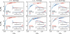 |
Fig. 1 Phase-space distribution of stars in the 1Ps and 2Ps for the models N2M and N05M at different times. At t = 0 Gyr, both clusters show a similar relative distribution of stars in the 1Ps (red) and 2Ps (blue), due to their similar half-mass radius and mass ratios. As the clusters evolve, the 2P expands towards the regions initially dominated by the 1P. By t = 12 Gyr, the N2M model is still partially mixed, while the N05M model has a significant degree of mixing. The insets show the marginalised distribution of energy and angular momentum, likewise highlighting the evolution of dynamical mixing. In all panels, the dashed lines follow the maximum allowed angular momentum at a given energy, defined by the angular momentum of the circular orbit of the corresponding energy. |
3 Signatures of phase-space mixing
We studied the degree of dynamical mixing by tracing the time evolution of the distribution function (DF) for each stellar population. The simulations we used are spherically symmetric, and therefore, we expected the DF to be only a function of the energy (E) and total angular momentum (L = |L|). We identified the DF of each population as F1P(E, L) for the initially extended 1P population, and F2P(E, L) for the initially compact 2P population. As the cluster evolved, both populations, which were initially in different regions of the phase space of energy and angular momentum, diffused in phase space and eventually populated the same region. Once this occurred, we considered the populations to be fully mixed.
We followed the mixing of the stellar populations in each simulation by measuring the instantaneous energy and angular momentum per unit mass for each star every 100 Myr. We measured these values by taking the 3D positions and velocities of each star along with the potential energy given by the global mass distribution in the cluster:
![Mathematical equation: $\[E_i=0.5 \times\left(v_{r, i}^2+v_{\theta, i}^2+v_{\phi, i}^2\right)+\Phi\left(r_i\right),\]$](/articles/aa/full_html/2025/07/aa53155-24/aa53155-24-eq2.png) (2)
(2)
![Mathematical equation: $\[L_i=r_i \times \sqrt{v_{\phi, i}^2+v_{\theta, i}^2}.\]$](/articles/aa/full_html/2025/07/aa53155-24/aa53155-24-eq3.png) (3)
(3)
To compare simulations with different sizes and masses, we normalised the energy by Φh = 0.5GMtot/rh and the angular momentum by ![Mathematical equation: $\[L_{h}=\sqrt{0.5 G M_{\text {tot}} r_{h}}\]$](/articles/aa/full_html/2025/07/aa53155-24/aa53155-24-eq4.png) . Φh and Lh corresponds to the potential of a point mass of half of the total mass of the cluster at the distance of rh, and the angular momentum of the circular orbit at rh in the same point mass potential, respectively.
. Φh and Lh corresponds to the potential of a point mass of half of the total mass of the cluster at the distance of rh, and the angular momentum of the circular orbit at rh in the same point mass potential, respectively.
Figure 1 shows the DF of each stellar population for the simulated clusters with the lowest (N2M) and the highest (N05M) degree of mixing at three different epochs: 0 Gyr, 7 Gyr, and 12 Gyr. As described in Sect. 2, both clusters have different initial conditions but share the same relative ratios for each population’s half-mass radius and total masses, giving them similar normalised distributions in the phase space. Initially (t = 0), the 1P (red contours) is extended (larger values of L) and less concentrated (shallower total energy). Moreover, it occupies the upper regions of the phase space. The 2P (blue contours) is more concentrated and limited to the deepest part of the cluster’s potential. The inset panels show the initial difference between the configurations of both populations in the marginalised distributions of angular momentum and total energy. As the clusters evolve, both populations start to mix in phase space. The 2P ‘diffuses’ to larger energies and higher angular momentum values, a process also driven by the reduction of the potential caused by the cluster’s mass loss due to stellar evolution and stellar escape. The increase of the angular momentum values also goes hand in hand with the more extended orbits. At 7 Gyr (middle panel), we observe that model N2M still shows a significant difference between the two populations, while model N05M exhibits a higher degree of mixing, particularly in the energy distribution. The N05M model is also dynamically older with a dynamical age of nh(7 Gyr) = 4.9 compared to model N2M with nh(7 Gyr) = 1.0. At 12 Gyr, the populations in model N2M are still in the process of mixing. By contrast, both populations appear thoroughly mixed for model N05M, as the distributions of stars only show minor differences.
We constructed a grid on the energy-angular momentum space to quantify the differences in the distribution of both stellar populations. In each bin, we took the squared difference of the normalised distributions and then summed over all bins using
![Mathematical equation: $\[S^2=\sum_i^{N_L} \sum_k^{N_E}\left(\rho\left(L_i, E_k\right)_{2 P}-\rho\left(L_i, E_k\right)_{1 P}\right)^2 \times\left(N_L N_E\right),\]$](/articles/aa/full_html/2025/07/aa53155-24/aa53155-24-eq5.png) (4)
(4)
where ρ(Li, Ek)1P and ρ(Li, Ek)2P are the number of stars in each (i, k) bin normalised by the total number of stars in each population to make the distributions comparable. While the initial value of S2 might depend on the initial separation of the populations, as the populations mix, S2 tends to zero.
Figure 2 shows the evolution of S2 for all models in our sample as a function of time (panel a) and their dynamical age nh (panel b). At 12 Gyr, the models show clear diversity in the degree of mixing for the clusters. The model N2M shows the least mixing with S2 = 9.99, while the model N05M shows the most mixing at 12 Gyr with S2 = 0.52. In between these two extremes, we find two groups with similar S2: first, the models N2M-r10 (S2 = 4.07), N1M (S2 = 3.62), and N05M-wf (S2 = 3.59); second, the models N1M-r10 (S2 = 1.77) and N1M-ra (S2 = 1.61). All models follow a more similar evolutionary path of S2 with respect to the dynamical age nh (panel b). One substantial difference arises for the N2M model, where S2 increases around nh = 1, triggered by the cluster’s core collapse, which we discuss later in this section. The models N2M-r10 and N1M-r10 also follow a common evolutionary path; they begin with a less concentrated 2P and are initially more mixed. This translates to a lower initial value of S2. The N2M-r10 and N1M-r10 models follow a similar but parallel evolutionary path to the N2M, N1M and N05M models. The N05M and N1M-ra models start with comparable values of S2 as the N2M, N1M, and N05M-wf models, but the populations mix more rapidly.
3.1 Core collapse
Four models in our sample undergo core collapse within the 13 Gyr of evolution (see Fig. B.3). Among these, we see in Fig. 2 that the N2M model shows multiple peaks in S2. While not as strong, the N1M, N05M, and N05M-wf models also show a peak in S2 (panel a in Fig. 2). These peaks are consistent with the times of the first core collapse. Models N1M-ra, N2M-r10, and N1M-r10 do not undergo core collapse within the 13 Gyr of evolution.
We now discuss how the small peaks in S2 found in some of the simulations are the fingerprints of the evolution of the innermost regions at the time of core collapse, and how they relate to the degree of spatial mixing of the 1P and 2P populations in the cluster’s central regions at that time. The N2M model undergoes core collapse at t = 7.06 Gyr (nh(7.06 Gyr) = 0.97). At this time, the two populations do not show a significant mixing in phase space where the 2P dominates the cluster’s centre with a fraction of the total number of stars belonging to the 2P population within the 1Per cent Lagrangian radius equal to 0.87, while the global 2P fraction is equal to 0.52. Panel a in Fig. 3 shows the phase space at ~500 Myr before the first core collapse, showing that the populations are not yet mixed. On the other hand, the N05M model is considerably more mixed before it undergoes core collapse at t = 8.62 Gyr (nh(8.62 Gyr) = 7.46), as shown in panel b of Fig. 3. The N05M model has a central 2P fraction of f2P(r1%) = 0.63 and a global fraction of f2P = 0.6 at the time of the core collapse.
The difference in the central concentration of each population drives the observed small peaks in S2 during the core collapse. Panel c in Fig. 3 shows the value of S2 calculated using only the angular momentum distribution (i.e. marginalising over the energy space), S2(L), and the value of S2 calculated using only the energy distribution, S2(E). In both simulations, the time evolution of S2(L) does not show any feature associated with core collapse, whereas S2(E) for the N2M simulation is characterised by the same peaks associated with the core collapse and the subsequent core oscillations already revealed by the evolution of S2 in Fig. 2. As the core starts contracting in systems like the N2M models where 2P stars are the dominant population in the inner regions, more 2P stars follow the core contraction than 1P stars. This affects the potential energy distribution of the two populations and produces the observed peaks in S2 and S2(E). The strength of the peaks is determined by their degree of mixing: the further the system is from mixing, the more prominent are the peaks in S2 and S2(E).
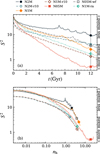 |
Fig. 2 Evolution of the S2 parameter for all models. Panel (a) shows the evolution of S2 with respect to the physical time in the simulations. All models show different degrees of mixing at most times. At t = 12 Gyr (vertical line), model N2M is the least mixed, while model N05M is the most mixed in phase space. Panel (b) shows the evolution of S2 as a function of the number of half-mass relaxation times. The symbols show the value of S2 at 12 Gyr and the respective number of relaxation times. |
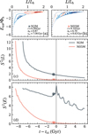 |
Fig. 3 Effects of partial mixing during core collapse. Panels a and b: phase-space distribution of the models N2M and N05M at ~500 Myr before core collapse. The N2M model is far from fully mixed, while the N05M model has a significant degree of mixing. Panel c: evolution of the S2 parameter centred at the time of core collapse for the models N2M and N05M (tcc = 7.06 Gyr and tcc = 8.62 Gyr). The markers indicate the corresponding time of phase-space distributions in panels a and b. Paneld shows the value of the S2 parameter only for the energy component of the phase space. The peaks in S2(E) show the effects of core collapse and subsequent core oscillations for the model N2M, where the 2P dominates the inner regions. While for N05M model, the two populations are almost completely mixed at the time of core collapse, and the evolution of S2(E) does not show any feature associated with the core collapse. |
3.2 Initially anisotropic model
The N1M and N1M-ra models start with the same initial conditions except for the initial radial anisotropy profile. The presence of primordial radial anisotropy impacts the overall evolution of the cluster. The N1M model has lost more mass and stars than the N1M-ra model. Furthermore, the N1M model undergoes core collapse at t = 7.54 Gyr, while the model N1M-ra continues to evolve towards core collapse at 13 Gyr. The delay of core collapse due to primordial velocity anisotropy has been thoroughly described by Breen et al. (2017) and Pavlík & Vesperini (2021) in the case of single-population clusters.
Figure 4 shows the S2 parameter, as in Fig. 2, for the N1M and N1M-ra models, as well as the marginalised distribution differences, S2(L) and S2(E). The N1M-ra model develops more dynamical mixing than the N1M model within their common range of dynamical ages. Two effects drive the difference in mixing as indicated by the S2 parameter. The initial velocity anisotropy in the N1M-ra model makes the angular momentum distribution for the 1P more compact and similar in extent to the 2P (see Fig. B.2). As the cluster evolves, the 2P develops radial anisotropy while the 1P slowly loses its anisotropy, becoming isotropic at about nh = 3 (see Fig. 8 and discussion therein). On the other hand, the N1M model evolves quickly to have a radially anisotropic 2P and a tangentially anisotropic 1P, adding to the differences in the angular momentum distribution. The second effect is the delayed core collapse, which allows the two populations in the N1M-ra model to spatially mix at a steady pace. In contrast, in the N1M, and as discussed in Sect. 3.1, the core collapse delays the energy mixing if one of the two populations dominates the core.
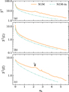 |
Fig. 4 Evolution of the S2 parameter (a), as well as S2 measured over the angular momentum (S2(L), panel b) and energy (S2(E), panel c) spaces for the N1M and N1M-ra models. Primordial radial anisotropy increases the population mixing rate while keeping the cluster dynamically younger. The model N1M-ra does not undergo core collapse within its 13 Gyr of evolution. |
4 Observable population mixing parameters derived from simulations
We discussed in Sect. 3 how differences in the phase-space distribution, traced by the S2 parameter, can help quantify the degree of dynamical mixing of the two populations in a GC. However, the S2 parameter can be measured only in numerical simulations. In this section, we explore three observable tracers for multi-population mixing, and we compare them with the S2 parameter.
Stars considered for the analysis presented in this section are limited to those brighter than two magnitudes below the turn-off magnitude. This limit encompasses the range of current observational data for multiple populations in GCs (see, e.g., Libralato et al. 2022; Martens et al. 2023; Cordoni et al. 2020, 2025). For each model, and at each time, we calculated the projected 2D radius (R) and the radial and tangential proper motions (vpmR, vpmT) for fifty different lines of sight.
The analysis of these ‘observables’ is not meant to be directly compared with observations but rather to illustrate how these measurements can trace the degree of dynamical mixing of the stellar populations and how they are linked to the phase-space mixing discussed in the previous sections. Therefore, we did not include kinematic errors or completeness effects, and we assumed that the two populations were clearly distinguishable with no 2P (1P) star misclassified as belonging to the 1P (2P) population.
4.1 Spatial differences
To quantify the differences in concentration and spatial distribution between the two populations, we used the A+parameter (Alessandrini et al. 2016; Lanzoni et al. 2016). The A+parameter measures the area difference between the cumulative stellar count of two samples of stellar tracers within a specific radial range [usually to measure the differences in the spatial distributions of populations with different masses, see, e.g., Alessandrini et al. (2016); Lanzoni et al. (2016) for a study using A+to measure the segregation of blue-stragglers relative to main-sequence and red giant stars, and Weatherford et al. (2018); Della Croce et al. (2024) for a study using A+to quantify the degree of mass segregation of more massive main sequence stars as well as the link between A+and the black hole content in GCs]. In our case, we followed a similar formulation for multiple populations as the one introduced by Dalessandro et al. (2018),
![Mathematical equation: $\[A^{+}\left(R_{\max }\right)=\int_0^1 \phi_{1 P}\left(R^{\prime}\right)-\phi_{2 P}\left(R^{\prime}\right) d R^{\prime},\]$](/articles/aa/full_html/2025/07/aa53155-24/aa53155-24-eq6.png) (5)
(5)
where ϕ(R′) is the cumulative radial distribution, R′ = R/Rmax, and Rmax is the maximum distance within which A+is calculated. In this work, we adopted Rmax = 2Rh. We also normalised the cumulative radial profile so that ϕ(Rmax) = 1.
Figure 5 shows the evolution of the ![Mathematical equation: $\[A_{2}^{+}\]$](/articles/aa/full_html/2025/07/aa53155-24/aa53155-24-eq7.png) parameter for all models as a function of time (panel a) and nh (panel b). If we look at a specific time, such as at 12 Gyr, we find that our models develop different degrees of spatial mixing: models N2M and N2M-r10 show the highest difference in concentration (more negative
parameter for all models as a function of time (panel a) and nh (panel b). If we look at a specific time, such as at 12 Gyr, we find that our models develop different degrees of spatial mixing: models N2M and N2M-r10 show the highest difference in concentration (more negative ![Mathematical equation: $\[A_{2}^{+}\]$](/articles/aa/full_html/2025/07/aa53155-24/aa53155-24-eq8.png) ), while model N05M exhibits the most spatial mixing of the models (
), while model N05M exhibits the most spatial mixing of the models (![Mathematical equation: $\[A_{2}^{+}\]$](/articles/aa/full_html/2025/07/aa53155-24/aa53155-24-eq9.png) ~0). On the other hand, if we look at the dynamical age nh, we find that the picture changes significantly. After nh ~ 1, all models converge, and differences between the
~0). On the other hand, if we look at the dynamical age nh, we find that the picture changes significantly. After nh ~ 1, all models converge, and differences between the ![Mathematical equation: $\[A_{2}^{+}\]$](/articles/aa/full_html/2025/07/aa53155-24/aa53155-24-eq10.png) parameter for the various models are less significant.
parameter for the various models are less significant.
It is interesting to note that the initial concentration differences between the r10 models and some of the r20 models mostly disappear by a dynamical age nh ~ 1–2. Moreover, in all the models, the initial spatial differences between 1Ps and 2Ps significantly decrease during the clusters’ early evolutionary phases. Even in dynamically young clusters (for example in clusters with nh ~ 1–3), these spatial differences are significantly smaller than those in the initial conditions imprinted by the formation process. These results show that the strength of present-day differences cannot be used to infer the extent of primordial differences and that even small present-day differences in dynamically young clusters may actually be the evolutionary outcome of multiple populations forming with strong dynamical differences [see also Tiongco et al. (2019); Vesperini et al. (2021); Sollima (2021) and the discussion in Cadelano et al. (2024)].
We do not find any clear signature of core collapse in the evolution of A+in Fig. 5. However, we can see some interesting behaviour if we look at the individual areas of the cumulative stellar distribution, particularly in the cluster centre (R < 0.5 Rh). In Fig. 6, we show the area of the cumulative stellar distribution within 0.5Rh for the models N2M (panel a) and N05M (panel b), following the comparison in Fig. 3. As we mentioned before in Sect. 3.1, the two populations in the N05M spatially mix before the cluster undergoes core collapse. At core collapse, the two populations increase their concentration at a similar rate. On the other hand, the model N2M is not spatially mixed by the time of core collapse, and 2P has a higher concentration than 1P, as shown by the larger value for the area of ϕ(R < 0.5Rh).
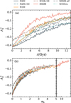 |
Fig. 5
|
![Mathematical equation: $\[A_{2}^{+}\]$](/articles/aa/full_html/2025/07/aa53155-24/aa53155-24-eq11.png)
4.2 Velocity anisotropy differences
In this section, we focus on the differences between the velocity anisotropy profiles of 1P and 2P stars. Several observational investigations of the velocity anisotropy profile of multiple populations have shown a 2P with varying degrees of radial anisotropy and a 1P that is isotropic or slightly tangential (see Bellini et al. 2015; Cordoni et al. 2020, 2025; Libralato et al. 2023; Dalessandro et al. 2024). Multiple studies investigating the evolution of the radial profiles of the velocity dispersion and anisotropy have shown that the observed velocity anisotropy profiles are consistent with those found in systems that assume initial conditions characterised by a tidally filling 1P system and a tidally underfilling 2P subsystem [see, e.g., Vesperini et al. (2021); Sollima (2021); Livernois et al. (2024); see also, e.g., Tiongco et al. (2016) and references therein for a similar evolution of the anisotropy in tidally filling and tidally underfilling single-population clusters].
With the goal of quantifying these differences, we adopted a new parameter that provides a global measure of the difference between the velocity anisotropy of the two populations by means of the area between the best-fitted velocity anisotropy models for 1P and 2P. We first calculated the velocity dispersion profiles for the radial and tangential components (projected on the sky) from the selected sample of stars. Then, we fitted a parametric model for the radial velocity dispersion and the velocity anisotropy. For the radial velocity dispersion, we used a fourth-order polynomial following the parameterisation in Watkins et al. (2022). For the tangential component, we used
![Mathematical equation: $\[\sigma_{\tan }^2=\sigma_{\mathrm{rad}}^2\left(1-\beta_{2 \mathrm{D}}\right),\]$](/articles/aa/full_html/2025/07/aa53155-24/aa53155-24-eq12.png) (6)
(6)
where we define the projected velocity anisotropy profile, ![Mathematical equation: $\[\beta_{2 \mathrm{D}}= 1-\sigma_{\tan }^{2} / \sigma_{\text {rad }}^{2}\]$](/articles/aa/full_html/2025/07/aa53155-24/aa53155-24-eq13.png) , with the parameterisation:
, with the parameterisation:
![Mathematical equation: $\[\beta_{2 \mathrm{D}}(R)= \begin{cases}\frac{\beta_i R^2}{\left(R_{\mathrm{a}}^2+R^2\right)}\left(1-\frac{R}{R_{\mathrm{t}}}\right) & \text { for } R<R_{\mathrm{t}} \\ 0 & \text { for } R \geq R_{\mathrm{t}}.\end{cases}\]$](/articles/aa/full_html/2025/07/aa53155-24/aa53155-24-eq14.png) (7)
(7)
This parameterisation is based on the Osipkov-Merrit velocity anisotropy profile (Osipkov 1979; Merritt 1985) with the anisotropy radius Ra, but allows for tangential anisotropy (βi < 0) and a maximum radial anisotropy smaller than max(β2D(R)) < 1. We also included a truncation term, (1 − R/Rt), so that the anisotropy profile could once again be isotropic (β2D = 0) at the truncation radius Rt. The truncation term allows us to properly characterise our simulations’ velocity anisotropy profile at large radii. For the purpose of this analysis, we fixed the anisotropy truncation radius at the respective tidal radius of each simulated cluster’s snapshot. We then calculated the anisotropy area Aβ for each population by first normalising the radius with the tidal radius and then integrating over β2D(R).
Panels a and b in Fig. 7 show the best-fit velocity anisotropy profiles for the N2M model at two different times (t = 4 Gyr and t = 12 Gyr, respectively). At 4 Gyr, the 2P shows radial anisotropy with an anisotropy area of Aβ,2P = 0.282, while the 1P is close to being isotropic with Aβ,1P = 0.011. At 12 Gyr the 2P becomes slightly less radially anisotropic with Aβ,2P = 0.235, and the 1P is now tangentially anisotropic with Aβ,1P = −0.132. In panel (c), we show the time evolution of the anisotropy areas for model N2M. Both populations began isotropic with Aβ = 0; during the first 100 Myr of evolution, both populations developed radial anisotropy (with a stronger anisotropy for the 2P). The development of radial anisotropy follows early mass loss due to stellar evolution, followed by a shallowing of the potential and an expansion of the cluster. The difference in strength of radial anisotropy is a consequence of the initial extension of the populations and the tidally filling and underfilling conditions for the 1Ps and 2Ps, respectively. As the cluster evolves, the 2P steadily loses radial anisotropy, while the 1P becomes isotropic and then develops tangential anisotropy.
Panel d in Fig. 7 shows the anisotropy area difference between the populations for the N2M model. This difference is defined as
![Mathematical equation: $\[\Delta A_\beta=A_{\beta, 2 \mathrm{P}}-A_{\beta, 1 \mathrm{P}}.\]$](/articles/aa/full_html/2025/07/aa53155-24/aa53155-24-eq15.png) (8)
(8)
If both populations are close to isotropic (Aβ,2P ~ Aβ,1P ~ 0) or have similar anisotropy profiles (Aβ,2P ~ Aβ,1P ≠ 0), then ΔAβ is close to zero, we consider the populations to be kinematically mixed. On the other hand, as ΔAβ becomes different from zero, the populations are further from being mixed. This could be the case when 2P has a strong radial anisotropy, and 1P is isotropic (panel a in Fig. 7), or the two populations have opposite velocity anisotropy (as in panel b in Fig. 7, where 2P is radially anisotropic and 1P is tangentially anisotropic). We see that, for the N2M model, the anisotropy area difference remains relatively constant, which is consistent with it being the furthest from mixing at the end of the simulations.
We show the evolution of the anisotropy area for each population and the anisotropy difference for all models in Fig. 8. Our choice of initial conditions affects the populations differently. In panel a, the 1P for all models that are initially isotropic follows the same path: starting at Aβ = 0, developing a very mild radial anisotropy, becoming isotropic, and then developing tangential anisotropy. Only the N05M model returns to being close to isotropic at the end of the simulation. On the other hand, the N1M-ra model’s 1P begins with primordial radial anisotropy, which translates to an initial Aβ = 0.4. The cluster’s 1P proceeds to lose radial anisotropy and becomes isotropic at nh = 3. The evolution of the velocity anisotropy in the 1P is driven by its tidally filling condition and is consistent with tidally filling single population simulations (see, e.g., Tiongco et al. 2016). In panel b, the 2P shows two main paths of evolution driven by its initial concentration: as the 2P expands, clusters with an initially more concentrated 2P develop a more substantial radial anisotropy (Aβ ~ 0.4) than those with an initial concentration of r10 (Aβ ~ 0.3). As for the N1M-ra model, we note that, given the primordial velocity anisotropy profile of this model, the 2P stars populate mainly the inner isotropic regions, while the radial anisotropy mainly affects the 1P populations extending in the outer anisotropic regions.
In panel c of Fig. 8, we show the area difference for each model. Following the discussion for panels a and b, the imprint of the initial conditions is still present on the area difference. The initially isotropic models with r20 concentration develop a ΔAβ ~ 0.35 after the first 100 Myr, while the models with r10 develop a ΔAβ ~ 0.25. We see that for the two concentration groups, ΔAβ slowly decreases as the clusters become dynamically older, showing that differences in velocity anisotropy persist over several relaxation times. Only after nh = 6 does the N05M model show a continuous decline in ΔAβ, approaching complete kinematic mixing. On the other hand, the N1M-ra model has a ΔAβ = 0.05 after the first 100 Myr, starting in a ‘close to kinematic mixing’ state. This is because the 2P develops radial anisotropy, while the 1P was already radially anisotropic. As the cluster evolves dynamically and the 1P becomes isotropic, the ΔAβ value of the N1M-ra model increases and becomes similar to those with an initial concentration of r10. By the end of the simulation, as the 1P of the N1M-ra model becomes tangentially anisotropic, its ΔAβ value becomes consistent with the r20 models.
In Dalessandro et al. (2024), we estimated the anisotropy area (referred to as αβ in that paper) and the anisotropy area difference (referred to as ![Mathematical equation: $\[\left(\alpha_{\beta}^{S P}-\alpha_{\beta}^{F P}\right)\]$](/articles/aa/full_html/2025/07/aa53155-24/aa53155-24-eq16.png) in that paper) for a sample of Galactic GCs based on their observed kinematics, using the same definitions described here. We presented the N1M, N1M-ra, and N05M models to compare simulations with observations. Interestingly, we find a consistent trend between the observations and simulations in the evolution of these quantities. While further comparisons of the observed GCs and the simulations are beyond the scope of our current sample of simulations, we stress here the usefulness of the anisotropy area difference to trace the mixing process.
in that paper) for a sample of Galactic GCs based on their observed kinematics, using the same definitions described here. We presented the N1M, N1M-ra, and N05M models to compare simulations with observations. Interestingly, we find a consistent trend between the observations and simulations in the evolution of these quantities. While further comparisons of the observed GCs and the simulations are beyond the scope of our current sample of simulations, we stress here the usefulness of the anisotropy area difference to trace the mixing process.
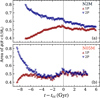 |
Fig. 6 Area of the cumulative stellar distribution within 0.5Rh (ϕ(<0.5Rh)) for the two populations in models: (a) N2M and (b) N05M. As in Fig. 3, we centre the time evolution at the respective time of the first core collapse. The two populations in model N2M have not achieved complete spatial mixing and ϕ2P(R < 0.5Rh) > ϕ1P(R < 0.5Rh). The model N05M has already attained a significant spatial mixing and ϕ2P(R < 0.5Rh) ~ ϕ1P(R < 0.5Rh). Furthermore, for model N05M, both populations show the same rate of increased concentration at core collapse, which explains the lack of signatures in S2(E) (see Fig. 3). |
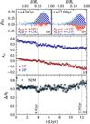 |
Fig. 7 Velocity anisotropy area (Aβ) and area difference (ΔAβ) for the N2M model. Panels a and b show the velocity anisotropy for the two populations (red upper triangles, PO1P, and downwards blue triangles, PO2P) in the N2M model at 4 Gyr and 12 Gyr, respectively. The hatched regions represent the respective anisotropy area for each population from the best-fit velocity dispersion and anisotropy parameterisation (see main text). Panel c shows the evolution of the anisotropy areas for the two populations over time; as the 2P becomes less radially anisotropic, the 1P becomes tangentially anisotropic and keeps a constant difference with the 2P, as shown in panel d, where we show the evolution of the anisotropy area difference. The vertical lines in panels c and d represent the times for which we show the velocity anisotropy profiles in panels a and b. |
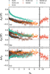 |
Fig. 8 Anisotropy area (Aβ) and area difference (ΔAβ) as described in Fig. 7, for all models in our sample with respect to their dynamical ages. For better visualisation, we separated nh into a linear section (nh ≤ 6) and a logarithmic section (nh > 6). |
4.3 Projected angular momentum differences
In Sect. 3, we showed that differences in the marginalised angular momentum can also trace kinematic mixing (see Figs. 1, 3, 4, and B.3). Furthermore, differences in the velocity anisotropy imply differences in the radial and tangential velocity dispersion components, which can manifest in the angular momentum distribution. As initially suggested in Sect. 3.2, stars on more radial orbits have smaller angular momentum at a given radius.
In this section, we explore the connection between the projected angular momentum Lz = vT × R (where vT is the tangential velocity on the plane of the sky, and R is the projected distance from the cluster’s centre), and the velocity anisotropy. In a non-rotating cluster, the Lz distribution at any given radius is centred at zero, and, therefore, we focused on the dispersion of the Lz distribution, σLz, as an observational tracer of the 3D angular momentum. As in Sect. 3, we normalised by the half-mass angular momentum Lh of a circular orbit in an equivalent point-mass potential.
In order to provide some initial guidance on the link between σLz and the cluster’s velocity anisotropy, we show in Fig. 9 the radial profile of σLz for four single-population King models with different radial anisotropy profiles built with the Limepy code (Gieles & Zocchi 2015, 2017). The value of σLz at a given radius in the cluster’s outer regions decreases for more radially anisotropic models. This decrease in σLz for more radially anisotropic velocity distributions is consistent with the expected smaller fraction of orbits with larger angular momentum (corresponding to a narrower distribution of Lz for more anisotropic models).
Following the correlations observed in the single-population King models, the differences in velocity anisotropy between the stellar populations discussed in Sect. 4.2 should also appear as differences in σLz. Fig. 10 shows the σLz profile for the two populations of the N2M and N05M models at 12 Gyr (panels a and b). The N2M model, which exhibits the largest velocity anisotropy area difference, also displays distinct σLz profiles, and as expected, σLz (1P) ≥ σLz (2P). The N05M model shows almost no differences between the σLz profiles, consistent with being close to complete mixing. Considering how the differences in σLz appear more significant outside of the half-light radius, we follow the time evolution of the difference between the 1P and 2P values of σLz at r = 2Rh for all epochs in our simulations. Panel c shows the time evolution of ΔσLz for models N2M and N05M. This plot shows that, as the cluster evolves and mixes, ΔσLz approaches zero and provides another tracer to measure the kinematic mixing of the two populations.
Figure 11 shows the evolution of ΔσLz for all the models in our sample in terms of physical time and dynamical age. The models N2M and N 05 M show the most and the least differences in σLz between the populations. The models with initial r10 concentration begin with smaller values of ΔσLz than the r20 models, and after 1 Gyr, the models with initial r10 concentration overlap with the N1M-ra model. The latter also moves to a larger difference in σLz, consistent with 1P evolving from a radially anisotropic state to isotropic and then tangentially anisotropic. As we examine the dynamical age, we see that the evolutionary paths change. Instead of exhibiting a set of parallel tracks, all the models converge into a single path. The models N1M-ra, N1M-r10, and N2M-r10 join at a single path at approximately nh = 0.1 early in the dynamical evolution of the clusters. As we measure the differences at 2Rh, we see degeneration between the effects of a weaker radially anisotropic 2P (N1M-r10 and N2M-r10) and two populations with different degrees of radial anisotropy (N1M-ra, the 1P becomes isotropic at nh = 3, see panel a in Fig. 8). The rest of the models follow a single path and begin to overlap at nh = 4. While most of our models do not get past this point, we expect them to follow the path of the N05M model.
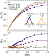 |
Fig. 9 Projected angular momentum dispersion σLz profiles for King models with different velocity anisotropy profiles (panel a) and their respective velocity anisotropy profiles (panel b). As the King models become more radially anisotropic (smaller values of ra/rh), the projected angular momentum dispersion decreases. The insets on panel a show the distribution of the projected angular momentum at r ~ 2Rh for the models with the most and the least radial anisotropy. The grey area in panel a shows the range of radial distances of stars used to calculate the histograms in the panel. We normalised σLz by the half-mass angular momentum Lh, corresponding to the angular momentum of a circular orbit of an equivalent point-mass potential (see Sect. 3). |
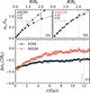 |
Fig. 10 Projected angular momentum dispersion σLz profiles for both populations in the N2M model (panel a) and the N05M model (panel b) at 12 Gyr. The vertical grey solid lines in panels a and b represent the difference in σLz between the populations at R = 2Rh. Panel c shows the time evolution of σLz difference at 2Rh; the closer this value is to zero, the closer the two populations are to kinematically mixing. |
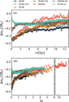 |
Fig. 11 Evolution of the projected angular momentum difference at 2Rh for all models in our sample as described in panel c of Fig. 10. In panel a, this is with respect to the physical time of the simulation, and in panel b this is with respect to their dynamical age. Once we consider the dynamical age, all models converge into the same evolutionary path, independently of their initial conditions. |
4.4 Connection with the S2 parameter
We explored three different observational parameters to quantify the degree of mixing of the multiple populations. All three trace different aspects of the mixing process: ![Mathematical equation: $\[A_{2}^{+}\]$](/articles/aa/full_html/2025/07/aa53155-24/aa53155-24-eq17.png) follows spatial mixing, whereas ΔAβ and ΔσLz trace differences in the velocity distribution anisotropy of the two populations and follow kinematic mixing. In Sect. 3, we defined the S2 parameter as a way to describe overall phase-space mixing. Now, we compare the S2 parameter – which cannot be observed directly – with the three observable tracers of mixing.
follows spatial mixing, whereas ΔAβ and ΔσLz trace differences in the velocity distribution anisotropy of the two populations and follow kinematic mixing. In Sect. 3, we defined the S2 parameter as a way to describe overall phase-space mixing. Now, we compare the S2 parameter – which cannot be observed directly – with the three observable tracers of mixing.
Figure 12 shows the three projected quantities we analysed as a function of the S2 parameter, with increasing mixing, i.e. decreasing S2 towards the right. We find the exact overall behaviour when comparing each parameter with the dynamical time. As the clusters become more mixed (smaller value of S2), the observational parameters approach zero. However, we also distinguish additional features due to the cluster’s different evolutionary state. Panel a of Fig. 12 shows the effects of core collapse and the subsequent divergence into different evolutionary paths. This divergence is due to the degree of spatial mixing in the core at core collapse. The clusters that do not undergo core collapse do not show a temporary increase in S2 (corresponding to the bump shown in Fig. 2). In the case of the velocity anisotropy area difference in panel b, we see similar behaviour as in Fig. 8. Lastly, for the difference in the projected angular momentum in panel c, all the models begin to converge onto the same path after attaining a mixing level of S2 ≃ 9. It is important to note, however, that at this value of S2 ≃ 9, differences between models persist when examining the velocity anisotropy area difference.
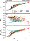 |
Fig. 12 Comparison of the three projected parameters that quantify the degree of mixing of the multiple populations with the S2 parameter from the phase-space mixing. The S2 parameter decreases to the right following the increasing phase-space mixing of the two populations, as stated at the top of the panel a. |
5 Discussion and summary
In this work, we analysed the long-term evolution of simulations with multiple populations to characterise the dynamical mixing process. Our simulations follow the evolution of models with an initially concentrated and underfilling 2P in an extended, more massive, and tidally filling 1P. We explored different initial conditions to examine differences in the concentration of the 2P, the primordial velocity anisotropy of the cluster, and the strength of the tidal field.
Multiple studies have shown that the different stellar populations in GCs have a large variety of spatial and kinematic mixing as traced by differences in concentration (see, e.g., Dalessandro et al. 2019; Leitinger et al. 2023; Cadelano et al. 2024), rotation (see, e.g., Cordero et al. 2017; Cordoni et al. 2020; Dalessandro et al. 2021, 2024; Martens et al. 2023; Leitinger et al. 2025), and velocity anisotropy (see, e.g., Richer et al. 2013; Bellini et al. 2015; Cordoni et al. 2020, 2025; Libralato et al. 2023; Dalessandro et al. 2024). To trace the evolution of the mixing processes, we followed the differences in the phase-space distribution of each population in our models. We defined the S2 parameter as the sum of the energy and angular momentum distribution square differences over the whole phase space. The S2 parameter allows us to build a comprehensive dynamical picture of the mixing process, including both the spatial and kinematic components of the populations mixing. We find that (as expected) mixing increases with dynamical age (see Fig. 2). We also show that core collapse and primordial velocity anisotropy can alter the mixing rate of the cluster, and core collapse may even cause a temporary slight inversion of the phase-space mixing (see Figs. 3 and 4). As shown in Fig. 2, models can achieve similar values of S2 at different physical and dynamical ages, either due to variations in their mixing rates or initial conditions. Our models reach different degrees of dynamical mixing at 12 Gyr; among all the models presented, the N05M and N2M exhibit, respectively, the most and the least mixing.
We followed the evolution of three “observable” parameters that can trace the degree of spatial and kinematic mixing and found that they display the same general trends as in previous observational studies (see, e.g., Dalessandro et al. 2019, 2024; Cadelano et al. 2024), where the differences in the spatial and kinematic properties of multiple populations decrease with dynamical age. We also find that in our models, the strength of the initial 1P and 2P differences already decreases in the clusters’ early evolutionary phases when the clusters are still dynamically young (nh ~ 1–2) (see also Vesperini et al. 2021; Sollima 2021; Cadelano et al. 2024). Present-day differences still contain important information about the 1P and 2P dynamical properties imprinted at the time of cluster formation. However, it is important to note that the observed present-day strength of these differences can be much smaller than the initial ones, even in dynamically young clusters, and that different initial conditions may lead to similar present-day properties. Furthermore, and as a cautionary note, our data do not consider limitations typically affecting observational analyses, such as incompleteness or uncertainties in population membership, which can add stochasticity to the evolutionary paths and reduce the detected spatial differences shown in Fig. 5.
We quantified the difference in the velocity anisotropy profiles of each population with the ΔAβ parameter, which measures the area difference between the velocity anisotropy profiles. This parameter is the most lasting kinematic signature for mixing, as the models still keep differences after multiple relaxation times. The overall trend is driven by a radially anisotropic 2P and a tangentially anisotropic 1P. For all the initially isotropic models, the 1P remains isotropic in the inner regions and develops tangential anisotropy in the outer regions, while 2P evolves towards a radially anisotropic velocity distribution with the strength of radial anisotropy depending on the initial concentration of 2P: initially less concentrated 2P spatial distributions results into a shallower radial velocity anisotropy (see Fig. 8). The model with an initial radially anisotropic velocity distribution illustrates the complexity of the interplay between the effects due to different spatial and velocity distributions. In the initially anisotropic model we studied (N1M-ra with rh,1P/rh2,P = 20), the difference between 1P and 2P anisotropy, after nh ~ 1, evolves similarly to that of an initially isotropic model but with smaller initial spatial differences (N1M-r10). Additional models are necessary to further explore these aspects of the clusters’ dynamical mixing.
Finally, we studied the evolution of σLz, the dispersion of the angular momentum calculated from the tangential component of the proper motion velocity on the plane of the sky and the projected radial distance from the cluster’s centre. We show that this parameter is linked to the degree of radial anisotropy, and that the differences between the values of this parameter for 1P and 2P, ΔσLz, trace the differences in the degree of anisotropy of their velocity distributions. More importantly, this parameter allows for a more direct way to quantify differences in the velocity distribution of the two populations and provides another observational measure of the kinematics of multiple populations, as well as the degree of kinematic mixing. We explored its evolutionary path (see Figs. 10 and 11) as well as its co-evolution with global phase-space mixing measured by S2 (see Fig. 12). For dynamical ages nh ≳ 1–2, the evolutionary paths of ΔσLz for models with different initial conditions approach a common universal track. As pointed above, dynamical differences observed in old clusters provide key information on the differences between the 1P and 2P spatial and kinematic properties set by formation processes and their evolution. However, even for dynamically young clusters, it is necessary to exercise caution in interpreting the specific strength of present-day differences as a close indication of those imprinted at the time of multiple population formation.
Models extending the investigation presented here to a broader set of initial conditions are necessary to further explore the evolutionary path of the parameters introduced in this paper, as well as their link to the clusters’ initial conditions. Including other dynamical indicators, such as differences in the degree of energy equipartition and internal rotation, will provide additional key steps towards a comprehensive picture of the dynamical mixing of multiple populations in GCs.
Acknowledgements
EV and FA acknowledge support from STScI grant AR-16157. EV acknowledges also support from the John and A-Lan Reynolds Faculty Research Fund. ED acknowledges financial support from the Fulbright Visiting Scholar program 2023. ED is also grateful for the warm hospitality of Indiana University, where part of this work was performed. This research was supported in part by Lilly Endowment, Inc., through its support for the Indiana University Pervasive Technology Institute. FA also acknowledges the following Python packages used during the research presented here: NumPy (Harris et al. 2020), SciPy (Virtanen et al. 2020), emcee (Foreman-Mackey et al. 2013) and Astropy (Astropy Collaboration 2022), while all figures were made using Matplotlib (Hunter 2007).
Appendix A Simulation properties at 7 Gyr and 12 Gyr
Properties at t = 7 Gyr
Properties at t = 12 Gyr
Appendix B Additional figures
We include in this appendix three additional figures to complement Figures 1 and 2. Figures B.1 and B.2 show the phase-space distribution for all models at t = 0, 4, 8, 12 Gyr, while Fig. B.3 shows the S2 parameter (as in Fig. 2) and the corresponding marginalised version for angular momentum S2(L) and energy S2(E).
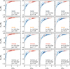 |
Fig. B.1 Phase-space distribution evolution for models N2M, N1M, N05M and N05M-wf at t = 0 Gyr, t = 4 Gyr, t = 7 Gyr and t = 12 Gyr. For each model, we include the corresponding dynamical age traced by the number of half-mass relaxation times nh. |
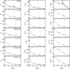 |
Fig. B.3 Time evolution of the S2 parameter for all models as in panel (a) in Fig. 2, but separated and also including the marginalisation over angular momentum S2(L) and energy S2(E). We have marked a vertical line at the time of the first core collapse for all models that undergo core collapse within the 13 Gyr of evolution. |
References
- Alessandrini, E., Lanzoni, B., Ferraro, F. R., Miocchi, P., & Vesperini, E. 2016, ApJ, 833, 252 [NASA ADS] [CrossRef] [Google Scholar]
- Amaro-Seoane, P., Konstantinidis, S., Brem, P., & Catelan, M. 2013, MNRAS, 435, 809 [Google Scholar]
- Astropy Collaboration (Price-Whelan, A. M., et al.) 2022, ApJ, 935, 167 [NASA ADS] [CrossRef] [Google Scholar]
- Bastian, N., & Lardo, C. 2018, ARA&A, 56, 83 [Google Scholar]
- Bekki, K. 2010, ApJ, 724, L99 [CrossRef] [Google Scholar]
- Bekki, K. 2011, MNRAS, 412, 2241 [NASA ADS] [CrossRef] [Google Scholar]
- Bellini, A., Vesperini, E., Piotto, G., et al. 2015, ApJ, 810, L13 [NASA ADS] [CrossRef] [Google Scholar]
- Berczik, P., Panamarev, T., Ishchenko, M., & Kocsis, B. 2025, A&A, 694, A163 [NASA ADS] [CrossRef] [EDP Sciences] [Google Scholar]
- Breen, P. G., Varri, A. L., & Heggie, D. C. 2017, MNRAS, 471, 2778 [NASA ADS] [CrossRef] [Google Scholar]
- Cadelano, M., Dalessandro, E., & Vesperini, E. 2024, A&A, 685, A158 [NASA ADS] [CrossRef] [EDP Sciences] [Google Scholar]
- Cai, M. X., Gieles, M., Heggie, D. C., & Varri, A. L. 2016, MNRAS, 455, 596 [NASA ADS] [CrossRef] [Google Scholar]
- Calura, F., D’Ercole, A., Vesperini, E., Vanzella, E., & Sollima, A. 2019, MNRAS, 489, 3269 [Google Scholar]
- Cordero, M. J., Hénault-Brunet, V., Pilachowski, C. A., et al. 2017, MNRAS, 465, 3515 [NASA ADS] [CrossRef] [Google Scholar]
- Cordoni, G., Milone, A. P., Mastrobuono-Battisti, A., et al. 2020, ApJ, 889, 18 [Google Scholar]
- Cordoni, G., Casagrande, L., Milone, A. P., et al. 2025, MNRAS, 537, 2342 [Google Scholar]
- Dalessandro, E., Cadelano, M., Vesperini, E., et al. 2018, ApJ, 859, 15 [NASA ADS] [CrossRef] [Google Scholar]
- Dalessandro, E., Cadelano, M., Vesperini, E., et al. 2019, ApJ, 884, L24 [Google Scholar]
- Dalessandro, E., Raso, S., Kamann, S., et al. 2021, MNRAS, 506, 813 [CrossRef] [Google Scholar]
- Dalessandro, E., Cadelano, M., Della Croce, A., et al. 2024, A&A, 691, A94 [NASA ADS] [CrossRef] [EDP Sciences] [Google Scholar]
- Della Croce, A., Aros, F. I., Vesperini, E., et al. 2024, A&A, 690, A179 [NASA ADS] [CrossRef] [EDP Sciences] [Google Scholar]
- D’Ercole, A., Vesperini, E., D’Antona, F., McMillan, S. L. W., & Recchi, S. 2008, MNRAS, 391, 825 [CrossRef] [Google Scholar]
- Foreman-Mackey, D., Hogg, D. W., Lang, D., & Goodman, J. 2013, PASP, 125, 306 [Google Scholar]
- Fregeau, J. M., Cheung, P., Portegies Zwart, S. F., & Rasio, F. A. 2004, MNRAS, 352, 1 [CrossRef] [Google Scholar]
- Gavagnin, E., Mapelli, M., & Lake, G. 2016, MNRAS, 461, 1276 [NASA ADS] [CrossRef] [Google Scholar]
- Gieles, M., & Zocchi, A. 2015, MNRAS, 454, 576 [NASA ADS] [CrossRef] [Google Scholar]
- Gieles, M., & Zocchi, A. 2017, LIMEPY: Lowered Isothermal Model Explorer in PYthon, Astrophysics Source Code Library, [record http://www.ascl.net/1710.023] [Google Scholar]
- Gieles, M., Charbonnel, C., Krause, M. G. H., et al. 2018, MNRAS, 478, 2461 [Google Scholar]
- Giersz, M., & Heggie, D. C. 1996, MNRAS, 279, 1037 [NASA ADS] [Google Scholar]
- Giersz, M., Heggie, D. C., Hurley, J. R., & Hypki, A. 2013, MNRAS, 431, 2184 [NASA ADS] [CrossRef] [Google Scholar]
- Gratton, R. G., Carretta, E., & Bragaglia, A. 2012, A&A Rev., 20, 50 [NASA ADS] [CrossRef] [Google Scholar]
- Gratton, R., Bragaglia, A., Carretta, E., et al. 2019, A&A Rev., 27, 8 [NASA ADS] [CrossRef] [Google Scholar]
- Harris, C. R., Millman, K. J., van der Walt, S. J., et al. 2020, Nature, 585, 357 [NASA ADS] [CrossRef] [Google Scholar]
- Hénault-Brunet, V., Gieles, M., Agertz, O., & Read, J. I. 2015, MNRAS, 450, 1164 [CrossRef] [Google Scholar]
- Hénon, M. 1971a, Ap&SS, 13, 284 [Google Scholar]
- Hénon, M. H. 1971b, Ap&SS, 14, 151 [Google Scholar]
- Hunter, J. D. 2007, Comput. Sci. Eng., 9, 90 [NASA ADS] [CrossRef] [Google Scholar]
- Hurley, J. R., Pols, O. R., & Tout, C. A. 2000, MNRAS, 315, 543 [Google Scholar]
- Hurley, J. R., Tout, C. A., & Pols, O. R. 2002, MNRAS, 329, 897 [Google Scholar]
- Hypki, A., & Giersz, M. 2013, MNRAS, 429, 1221 [NASA ADS] [CrossRef] [Google Scholar]
- Hypki, A., Giersz, M., Hong, J., et al. 2022, MNRAS, 517, 4768 [NASA ADS] [CrossRef] [Google Scholar]
- Hypki, A., Vesperini, E., Giersz, M., et al. 2025, A&A, 693, A41 [NASA ADS] [CrossRef] [EDP Sciences] [Google Scholar]
- Ishchenko, M., Sobolenko, M., Berczik, P., et al. 2023, A&A, 678, A69 [NASA ADS] [CrossRef] [EDP Sciences] [Google Scholar]
- Khoperskov, S., Mastrobuono-Battisti, A., Di Matteo, P., & Haywood, M. 2018, A&A, 620, A154 [NASA ADS] [CrossRef] [EDP Sciences] [Google Scholar]
- King, I. R. 1966, AJ, 71, 64 [Google Scholar]
- Kroupa, P. 2001, MNRAS, 322, 231 [NASA ADS] [CrossRef] [Google Scholar]
- Lacchin, E., Calura, F., Vesperini, E., & Mastrobuono-Battisti, A. 2022, MNRAS, 517, 1171 [NASA ADS] [CrossRef] [Google Scholar]
- Lanzoni, B., Ferraro, F. R., Alessandrini, E., et al. 2016, ApJ, 833, L29 [NASA ADS] [CrossRef] [Google Scholar]
- Leitinger, E., Baumgardt, H., Cabrera-Ziri, I., Hilker, M., & Pancino, E. 2023, MNRAS, 520, 1456 [NASA ADS] [CrossRef] [Google Scholar]
- Leitinger, E. I., Baumgardt, H., Cabrera-Ziri, I., et al. 2025, A&A, 694, A184 [Google Scholar]
- Libralato, M., Bellini, A., Vesperini, E., et al. 2022, ApJ, 934, 150 [NASA ADS] [CrossRef] [Google Scholar]
- Libralato, M., Vesperini, E., Bellini, A., et al. 2023, ApJ, 944, 58 [CrossRef] [Google Scholar]
- Livernois, A. R., Aros, F. I., Vesperini, E., et al. 2024, MNRAS, 534, 2397 [Google Scholar]
- Martens, S., Kamann, S., Dreizler, S., et al. 2023, A&A, 671, A106 [NASA ADS] [CrossRef] [EDP Sciences] [Google Scholar]
- Mastrobuono-Battisti, A., & Perets, H. B. 2013, ApJ, 779, 85 [NASA ADS] [CrossRef] [Google Scholar]
- Merritt, D. 1985, AJ, 90, 1027 [Google Scholar]
- Milone, A. P., & Marino, A. F. 2022, Universe, 8, 359 [NASA ADS] [CrossRef] [Google Scholar]
- Osipkov, L. P. 1979, Pisma Astron. Zh., 5, 77 [Google Scholar]
- Pavlík, V., & Vesperini, E. 2021, MNRAS, 504, L12 [CrossRef] [Google Scholar]
- Richer, H. B., Heyl, J., Anderson, J., et al. 2013, ApJ, 771, L15 [NASA ADS] [CrossRef] [Google Scholar]
- Sollima, A. 2021, MNRAS, 502, 1974 [NASA ADS] [CrossRef] [Google Scholar]
- Spitzer, L. 1987, Dynamical Evolution of Globular Clusters (Princeton, N.J.: Princeton University Press) [Google Scholar]
- Tiongco, M. A., Vesperini, E., & Varri, A. L. 2016, MNRAS, 455, 3693 [Google Scholar]
- Tiongco, M. A., Vesperini, E., & Varri, A. L. 2019, MNRAS, 487, 5535 [NASA ADS] [CrossRef] [Google Scholar]
- Vesperini, E., McMillan, S. L. W., D’Antona, F., & D’Ercole, A. 2013, MNRAS, 429, 1913 [Google Scholar]
- Vesperini, E., Hong, J., Webb, J. J., D’Antona, F., & D’Ercole, A. 2018, MNRAS, 476, 2731 [NASA ADS] [CrossRef] [Google Scholar]
- Vesperini, E., Hong, J., Giersz, M., & Hypki, A. 2021, MNRAS, 502, 4290 [NASA ADS] [CrossRef] [Google Scholar]
- Virtanen, P., Gommers, R., Oliphant, T. E., et al. 2020, Nat. Methods, 17, 261 [Google Scholar]
- Wang, L., Kroupa, P., Takahashi, K., & Jerabkova, T. 2020, MNRAS, 491, 440 [Google Scholar]
- Watkins, L. L., van der Marel, R. P., Libralato, M., et al. 2022, ApJ, 936, 154 [CrossRef] [Google Scholar]
- Weatherford, N. C., Chatterjee, S., Rodriguez, C. L., & Rasio, F. A. 2018, ApJ, 864, 13 [NASA ADS] [CrossRef] [Google Scholar]
See these reviews for a discussion of observational studies of a subset of about 20% of the Galactic GCs showing evidence of a variation also in Fe.
All Tables
All Figures
|
Fig. 1 Phase-space distribution of stars in the 1Ps and 2Ps for the models N2M and N05M at different times. At t = 0 Gyr, both clusters show a similar relative distribution of stars in the 1Ps (red) and 2Ps (blue), due to their similar half-mass radius and mass ratios. As the clusters evolve, the 2P expands towards the regions initially dominated by the 1P. By t = 12 Gyr, the N2M model is still partially mixed, while the N05M model has a significant degree of mixing. The insets show the marginalised distribution of energy and angular momentum, likewise highlighting the evolution of dynamical mixing. In all panels, the dashed lines follow the maximum allowed angular momentum at a given energy, defined by the angular momentum of the circular orbit of the corresponding energy. |
| In the text | |
|
Fig. 2 Evolution of the S2 parameter for all models. Panel (a) shows the evolution of S2 with respect to the physical time in the simulations. All models show different degrees of mixing at most times. At t = 12 Gyr (vertical line), model N2M is the least mixed, while model N05M is the most mixed in phase space. Panel (b) shows the evolution of S2 as a function of the number of half-mass relaxation times. The symbols show the value of S2 at 12 Gyr and the respective number of relaxation times. |
| In the text | |
|
Fig. 3 Effects of partial mixing during core collapse. Panels a and b: phase-space distribution of the models N2M and N05M at ~500 Myr before core collapse. The N2M model is far from fully mixed, while the N05M model has a significant degree of mixing. Panel c: evolution of the S2 parameter centred at the time of core collapse for the models N2M and N05M (tcc = 7.06 Gyr and tcc = 8.62 Gyr). The markers indicate the corresponding time of phase-space distributions in panels a and b. Paneld shows the value of the S2 parameter only for the energy component of the phase space. The peaks in S2(E) show the effects of core collapse and subsequent core oscillations for the model N2M, where the 2P dominates the inner regions. While for N05M model, the two populations are almost completely mixed at the time of core collapse, and the evolution of S2(E) does not show any feature associated with the core collapse. |
| In the text | |
|
Fig. 4 Evolution of the S2 parameter (a), as well as S2 measured over the angular momentum (S2(L), panel b) and energy (S2(E), panel c) spaces for the N1M and N1M-ra models. Primordial radial anisotropy increases the population mixing rate while keeping the cluster dynamically younger. The model N1M-ra does not undergo core collapse within its 13 Gyr of evolution. |
| In the text | |
|
Fig. 5
|
| In the text | |
|
Fig. 6 Area of the cumulative stellar distribution within 0.5Rh (ϕ(<0.5Rh)) for the two populations in models: (a) N2M and (b) N05M. As in Fig. 3, we centre the time evolution at the respective time of the first core collapse. The two populations in model N2M have not achieved complete spatial mixing and ϕ2P(R < 0.5Rh) > ϕ1P(R < 0.5Rh). The model N05M has already attained a significant spatial mixing and ϕ2P(R < 0.5Rh) ~ ϕ1P(R < 0.5Rh). Furthermore, for model N05M, both populations show the same rate of increased concentration at core collapse, which explains the lack of signatures in S2(E) (see Fig. 3). |
| In the text | |
|
Fig. 7 Velocity anisotropy area (Aβ) and area difference (ΔAβ) for the N2M model. Panels a and b show the velocity anisotropy for the two populations (red upper triangles, PO1P, and downwards blue triangles, PO2P) in the N2M model at 4 Gyr and 12 Gyr, respectively. The hatched regions represent the respective anisotropy area for each population from the best-fit velocity dispersion and anisotropy parameterisation (see main text). Panel c shows the evolution of the anisotropy areas for the two populations over time; as the 2P becomes less radially anisotropic, the 1P becomes tangentially anisotropic and keeps a constant difference with the 2P, as shown in panel d, where we show the evolution of the anisotropy area difference. The vertical lines in panels c and d represent the times for which we show the velocity anisotropy profiles in panels a and b. |
| In the text | |
|
Fig. 8 Anisotropy area (Aβ) and area difference (ΔAβ) as described in Fig. 7, for all models in our sample with respect to their dynamical ages. For better visualisation, we separated nh into a linear section (nh ≤ 6) and a logarithmic section (nh > 6). |
| In the text | |
|
Fig. 9 Projected angular momentum dispersion σLz profiles for King models with different velocity anisotropy profiles (panel a) and their respective velocity anisotropy profiles (panel b). As the King models become more radially anisotropic (smaller values of ra/rh), the projected angular momentum dispersion decreases. The insets on panel a show the distribution of the projected angular momentum at r ~ 2Rh for the models with the most and the least radial anisotropy. The grey area in panel a shows the range of radial distances of stars used to calculate the histograms in the panel. We normalised σLz by the half-mass angular momentum Lh, corresponding to the angular momentum of a circular orbit of an equivalent point-mass potential (see Sect. 3). |
| In the text | |
|
Fig. 10 Projected angular momentum dispersion σLz profiles for both populations in the N2M model (panel a) and the N05M model (panel b) at 12 Gyr. The vertical grey solid lines in panels a and b represent the difference in σLz between the populations at R = 2Rh. Panel c shows the time evolution of σLz difference at 2Rh; the closer this value is to zero, the closer the two populations are to kinematically mixing. |
| In the text | |
|
Fig. 11 Evolution of the projected angular momentum difference at 2Rh for all models in our sample as described in panel c of Fig. 10. In panel a, this is with respect to the physical time of the simulation, and in panel b this is with respect to their dynamical age. Once we consider the dynamical age, all models converge into the same evolutionary path, independently of their initial conditions. |
| In the text | |
|
Fig. 12 Comparison of the three projected parameters that quantify the degree of mixing of the multiple populations with the S2 parameter from the phase-space mixing. The S2 parameter decreases to the right following the increasing phase-space mixing of the two populations, as stated at the top of the panel a. |
| In the text | |
|
Fig. B.1 Phase-space distribution evolution for models N2M, N1M, N05M and N05M-wf at t = 0 Gyr, t = 4 Gyr, t = 7 Gyr and t = 12 Gyr. For each model, we include the corresponding dynamical age traced by the number of half-mass relaxation times nh. |
| In the text | |
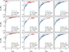 |
Fig. B.2 As in Fig. B.1, but for models N1M-ra, N2M-r10 and N1M-r10. |
| In the text | |
|
Fig. B.3 Time evolution of the S2 parameter for all models as in panel (a) in Fig. 2, but separated and also including the marginalisation over angular momentum S2(L) and energy S2(E). We have marked a vertical line at the time of the first core collapse for all models that undergo core collapse within the 13 Gyr of evolution. |
| In the text | |
Current usage metrics show cumulative count of Article Views (full-text article views including HTML views, PDF and ePub downloads, according to the available data) and Abstracts Views on Vision4Press platform.
Data correspond to usage on the plateform after 2015. The current usage metrics is available 48-96 hours after online publication and is updated daily on week days.
Initial download of the metrics may take a while.