| Issue |
A&A
Volume 699, July 2025
|
|
|---|---|---|
| Article Number | A7 | |
| Number of page(s) | 18 | |
| Section | Astronomical instrumentation | |
| DOI | https://doi.org/10.1051/0004-6361/202452444 | |
| Published online | 01 July 2025 | |
In-flight cross-calibration of HRIEUV/EUI and AIA/SDO
1
Solar-Terrestrial Centre of Excellence–SIDC, Royal Observatory of Belgium,
Ringlaan -3- Avenue Circulaire,
1180
Brussels,
Belgium
2
Centre Spatial de Liège, Université de Liège,
Av. du Pré-Aily B29,
4031
Angleur,
Belgium
3
Skobeltsyn Institute of Nuclear Physics, Moscow State University,
119991
Moscow,
Russia
4
Université Paris-Saclay, CNRS, Institut d’Astrophysique Spatiale,
91405
Orsay,
France
5
Faculty of Aerospace Engineering, Delft University of Technology,
2600
Delft,
The Netherlands
★ Corresponding author: This email address is being protected from spambots. You need JavaScript enabled to view it.
Received:
1
October
2024
Accepted:
11
April
2025
Abstract
Context. The extreme ultraviolet High-Resolution Imager (HRIEUV) of the Extreme Ultraviolet Imager (EUI) telescope on board Solar Orbiter observes the solar corona in an ~5 Å wide passband near 174 Å with unprecedented high spatial resolution.
Aims. We aim to perform radiometric cross-calibration of the HRIEUV and the Atmospheric Imaging Assembly (AIA) telescope in order to allow further mutual analyses of the observational data.
Methods. We applied a differential emission measure analysis using quasi-simultaneous images taken in seven spectral channels –HRIEUV and six channels of AIA – and compared the real and the simulated images.
Results. The comparison suggests that the real HRIEUV images have ~40% larger signal than the simulated images predicted by the differential emission measure analysis.
Conclusions. With our method we cannot conclude which instrument has errors in the absolute calibration, as it can be the case for either of them or both of them simultaneously, but to a lesser degree. However, in order to improve the accuracy of simultaneous data analysis, one needs to take this discrepancy into account. We see that introduction of the HRIEUV signal into the DEM analysis modifies the warm plasma with 1 MK. The ability of the method to reproduce HRIEUV images using only the AIA data further validates the underlying assumptions and our approach. Lastly, we believe the approach can be used as a strategy to establish a golden reference of contemporary EUV imagers.
Key words: techniques: photometric / telescopes / Sun: corona / Sun: UV radiation
© The Authors 2025
 Open Access article, published by EDP Sciences, under the terms of the Creative Commons Attribution License (https://creativecommons.org/licenses/by/4.0), which permits unrestricted use, distribution, and reproduction in any medium, provided the original work is properly cited.
This article is published in open access under the Subscribe to Open model. This email address is being protected from spambots. You need JavaScript enabled to view it. to support open access publication.
1 Introduction
The Extreme Ultraviolet Imager (EUI) instrument is a complex of three extreme ultraviolet (EUV) and Hydrogen Lyman-α telescopes (Rochus et al. 2020) on board the Solar Orbiter (SolO) spacecraft, launched on February 11, 2020. The EUI instrument includes the Full-Sun Imager (FSI) for EUV passbands near 174 Å and 304 Å, the high-resolution Hydrogen Lyman-α imager called HRILya , and the high-resolution EUV imager for the passband near 174 Å called HRIEUV.
The HRIEUV is based on off-axis Cassegrain layout and has an angular resolution of ~0.5 arcsec. Due to the unique orbit of the Solar Orbiter and its proximity to the Sun during part of the orbit, the HRIEUV delivers unprecedented spatial resolution on the order of a few hundred kilometers. A lot of small-scale and fast-dynamic phenomena and structures have already been observed, such as campfires (Berghmans et al. 2021), picojets (Chitta et al. 2023), decayless kink oscillations (Shrivastav et al. 2024), rotational movements (Petrova et al. 2024), and so on. Using simultaneous observations of other telescopes in addition to HRIEUV can provide additional advantages. In particular, Zhukov et al. (2021) used observations of HRIEUV and the Atmospheric Imaging Assembly telescope (AIA; Lemen et al. 2012) to measure the height of small-scale campfires in the solar atmosphere using stereoscopy. Berghmans et al. (2021) determined thermal properties of the observed campfires.
Simultaneous observations can also be used to verify radiometric calibration or intercalibration of the telescopes and/or spectrographs. In particular, Boerner et al. (2014) performed intercalibration of the AIA telescope with the EVE (EUV Variability Experiment; Woods et al. 2012) and EIS (EUV Imaging Spectrometer; Culhane et al. 2007) spectrographs. Hock & Eparvier (2008) performed absolute calibration of the EIT telescope (Extreme-Ultraviolet Imaging Telescope; Delaboudinière et al. 1995) on board Solar and Heliospheric Observatory using spectral irradiance of the Sun measured by the SEE instrument (Solar EUV Experiment) on board TIMED (Thermosphere Ionosphere Mesosphere Energetics and Dynamics) mission, while Shestov et al. (2014) derived radiometric calibration of the SPIRIT spectroheliograph using EIT images. Raftery et al. (2013) compared signals of several telescopes in the 171 Å passband, in particular AIA; SWAP (Sun Watcher with Active Pixels and Image Processing; Seaton et al. 2013) on board PROBA2 mission; EIT; and EUVI (Extreme ultraviolet Imager; Howard et al. 2008) on board STEREO for various isothermal and multi-thermal plasmas.
The relatively narrow passband of the spectral sensitivity of most of the EUV telescopes and complexity of the solar emission spectrum make the radiometric calibration and interpretation of the observed data quite cumbersome. The spectral lines of different ions are often very close together. Their intensity depends on temperature and density of plasma and can vary over a very wide range. Therefore, when a telescope registers an image, it may happen that the measured signal changes little, even if one or several spectral lines have become significantly brighter; on the contrary, a situation may occur whereby the measured signal has changed significantly, while the total radiation energy in the spectral range has not changed much. Commonly, the measured digital signal I in units [DN s−1] is interpreted using the concept of either emission measure in an isothermal model or differential emission measure (DEM; Pottasch 1964) in a multi-thermal model. In the first case, the signal is expressed as
 (1)
(1)
in the case of multi-temperature plasma, it is expressed as
 (2)
(2)
In these two equations, j denotes either a telescope or a passband of a multi-passband telescope, EMT0 [cm−5] and DEM(T) [cm−5 K−1] denote emission measure and differential emission measure of the emitting plasma, and Gj(T) [DN cm5 s−1] denotes the so-called temperature response function of the telescope. The function Gj(T) is calculated as an integral over λ of the product of the coronal spectral emissivity sT (λ) [photon s−1 cm3 sr-1 Å−1] per unit emission measure at temperature T and the telescope spectral response function Rj(λ) [DN sr cm2 photon−1]. The latter represents the main calibration characteristic of a telescope and is calculated as a product of the aperture size, the pixel solid angle, the spectral throughput of the optics, and the spectral sensitivity of the detector.
After observations in N different passbands or telescopes are available, we can build a system of N integral Equation (2) (j = 1, ..., N) and solve it to derive the unknown function DEM(T) Various approaches to solving the system exist, but in general all of them try to optimize the DEM(T) such that the simulated signals Ij match the measured ones as well as possible.
An important feature of the emission measure concept is that it allows us to separate the quantity of the emitting plasma, which is expressed by EMT0 or DEM(T) and all the other factors. These factors are expressed by Gj(T), which ultimately include all the characteristics of the telescopes and some plasma parameters such as chemical abundances and the kinetic rates of ionization and recombination and rates of level population and depopulation. As such, the emission measure approach allows us to analyze not only the observations of a multi-passband telescope, but also observations done by several different telescopes, including those that observe the solar corona from different vantage points, and have completely different spectral responses, aperture sizes, pixel plate scales, and so on. All these differences are accounted for by the corresponding Gj(T) functions, while the derived DEM(T) will only characterize the plasma of the solar corona. That is why temperature response functions Gj(T) are also frequently considered as calibration characteristics of telescopes along with their spectral response functions Rj(λ).
The temperature response functions Gj(T) cannot be measured in laboratory, because it is impossible to reproduce the solar EUV emission spectrum. Instead, during the on-ground calibrations the spectral response functions are measured, and afterwards Gj(T) are calculated using an available spectral model, such as that provided by the CHIANTI software (Del Zanna et al. 2021; Dere et al. 1997).
Potential errors both in the measured spectral response curves and in the emission-spectra model may introduce errors in the final function Gj(T). The errors in Gj(T) will, in turn, affect interpretation of the observed data: during the DEM-inversion procedure the errors in Gj(T) will result in systematic discrepancies of the predicted signals Ij, worsen the correspondence of the predicted and the measured signals, and, as a consequence, will introduce errors in the derived DEM. Thus, from the mutual DEM analysis of several telescopes one can infer the level of the correspondence of their Gj(T)s or, in other words, check their intercalibration. Systematic deviations of the signal of one of the telescopes will suggest the over- or underestimation of its Gj(T). A simple correction by an empirical factor  can improve the simulated/observed ratio and improve the DEM convergence. In addition, the intercalibration of several telescopes based on the in-flight data can not only verify the initial calibration accuracy, but also show potential in-orbit degradation of sensitivity.
In the present analysis, we perform intercalibration of the HRIEUV telescope and the AIA telescope. The present paper is structured as follows: in Sect. 2, we present the experimental data; and in Sect. 3, we describe the DEM-inversion and the data processing methods. The DEM analysis is performed in Sect. 4 using the AIA data only, and in Sect. 5 using mutual AIA and HRIEUV observations. Finally, in Sect. 6, we discuss the results.
2 Observations
The HRIEUV is based on an off-axis Cassegrain layout with an effective focal length of f = 4187 mm. A 10 μm complementary metal-oxide-semiconductor (CMOS) active-pixel-sensor (APS) image detector provides a pixel plate scale ≈0.5 arcsec/pixel. The entrance aperture Ø47.4 mm is situated in front of the telescope. The working passband is determined by a combination of its mirror coatings, filters, and detector spectral sensitivity. Periodic Al/Mo/SiC multilayer coating with the first order centered at 174 Å provides high peak reflectivity with the ~5 Å full width at half maximum (FWHM) passband. A fixed aluminum foil filter is situated between the entrance aperture and the primary mirror. A filter wheel with an open position, two identical aluminum filters, and an occulting slot is situated closer to the detector. On-ground calibrations of the HRIEUV are described in Gissot et al. (2023). We used the level-2 HRIEUV data, obtained with the aluminum filter, with the _hrieuv174- suffix in the file names and FILTER=’Aluminium_174_2’ as FITS keyword. In the current analysis, we used the images from the EUI Data Release 6.01 (Kraaikamp et al. 2023).
The AIA telescope is a set of four EUV and vacuum ultraviolet telescopes on board the Solar Dynamics Observatory mission (SDO; Pesnell et al. 2012). AIA uses Cassegrain optical layout with f = 4.125 m focal length, Ø20 cm primary mirrors each split into two zones with different coatings. The multilayer coatings for EUV spectral ranges provide ~10 Å FWHM passbands. The detectors are based on 12 μm back-side charge-coupled device (CCD), providing a pixel plate scale of 0.6 arcsec/pixel. AIA was extensively calibrated on-ground Boerner et al. (2012). During its in-orbit operations, several re-calibration campaigns were performed; degradation of the radiometric sensitivity was carefully analyzed (Boerner et al. 2014). In the current analysis, we use data from 6 AIA channels: 94, 131, 171, 193, 211, and 335 Å. We used the level-1.5 data obtained with aia_prep routines in SolarSoft (Freeland & Handy 1998). We took the degradation of the AIA radiometric sensitivity into account separately by corresponding factors in the temperature response functions.
For the analysis, we chose the observations performed on 30 May, 2020, 7 March, 2022, and 29 March, 2023. This almost three-year-period is sufficiently long for us to notice any possible degradation of either of the telescopes. On 30 May, 2020, the HRIEUV performed a high-cadence campaign, in which numerous small-scale brightenings or campfires were discovered and analyzed (Berghmans et al. 2021). The angular separation of SolO and the Earth on this date was relatively large - 31.3° -and even after re-projection, the parallax was noticeable in some structures. Thus, to reduce possible influence of the parallax, we used observations from 7 March, 2022 with the separation 3.0° and 29 March, 2023 with the separation 2.8°.
An example of the AIA 171 Å image and the HRIEUV 174 Å image re-projected to the AIA vantage point is given in Fig. 1. Both images were registered on 30 May, 2020 near 14:58 UT. Due to a relatively large angular separation of 31.3°, the field of view (FOV) of the HRIEUV view acquires some distortion during re-projection. There is a reasonably good correspondence of the structures in the re-projected images.
The spectral responses Rj(λ) of the AIA 171 Å channel and the HRIEUV telescope, as well as the emission spectra calculated for different temperatures, are given in Fig. 2. The top panel shows the normalized spectral responses of the telescopes. The AIA spectral sensitivity was obtained using the aia_get_response(/area,/dn,/full,/eve-norm,timedepend_date=..) routine. The HRIEUV spectral sensitivity included the spectral efficiency of the filters, mirrors, and detector; the aperture surface area; vignetting by the entrance and focal filter meshes; an additional 10% of vignetting by the supporting ribs of the filters; and, finally, the pixel solid angle. The second from top panel in Fig. 2 shows the emission spectra in the 160-210 Å region calculated with CHIANTI for different temperatures. The vertical axis corresponds to the logarithm of temperature and ranges from 105 K (log T = 5.0) to 40 MK (log T = 7.6), and the horizontal axis corresponds to that of the top panel. The color denotes intensity of the spectral line. The color scale is logarithmic, such that violet corresponds to half and red corresponds to one. We used the ch_synthetic and make_chianti_spec routines of v.10.1 CHIANTI with the sun_coronal_2021_chianti abundance and chianti.ioneq ionization equilibrium files and constant density ne = 109 cm−3 . The next two panels take into account spectral sensitivities of the telescopes. The horizontal and vertical axes are the same as on the previous panel. The AIA 171 Å spectral response is narrower and is centered on the FeIX 171 Å line. The L-edge of the Al-filter cuts the smooth spectral response of the multilayer optics near the peak, making the spectral response even narrower. The spectral response of the HRIEUV (shown in red) is wider than that of the AIA; it is centered on the Fe X 174.53 Å line. Due to its relatively large width the contribution of the Fe X 171 Å line is quite significant, as can be seen in the third panel. In the top panel, the spectral response of the FSI is shown in green, and the normalized spectrum is shown in gray (calculated for log T = 6.0) curves.
In order to obtain the temperature response functions Gj(T), we convolved the solar emission spectrum with the spectral responses Rj(λ) of the telescopes. We did not use the temperature responses of AIA provided by the aia_get_response() routine, available in SolarSoft for the following reason: during our analysis, we found that changes in the spectral emission model can change signal in a particular passband up to 50%, as compared to the previous spectral model. The changes of the ratio of the signals in different passbands are significantly smaller since the spectral model affects both passbands. In order to avoid any differences related to the applied spectral model, we calculated the temperature responses for all the channels of AIA and HRIEUV using the same parameters for CHIANTI. We used the 10-1000 Å wavelength range constant densities ne = 109 cm−3. We checked that using other densities or constant pressure p did not change the results; the curves for pressure p = const that correspond to ne = 109 cm−3 and T = 1 MK were almost indistinguishable from those calculated for ne = 109 cm−3. For AIA, the degradation obtained with aia_bp_get_corrections() was taken into account, which, for the period from 2020-2023, was constant and amounted to 0.9, 0.51, 0.74, 0.49, 0.40, and 0.17 for the spectral channels 94, 131, 171, 193, 211, and 335 Å2. The calculated temperature response functions Gj(T) are given in Fig. 3. The small difference in the spectral responses of the AIA 171 Å and HRIEUV makes their temperature responses G(T) very similar to each other in their shape, especially in logarithmic scale. The peak of the GA171(T) is shifted by Δ = 0.1 (in log T) to the left with respect to the GHRI(T); the drop at cold temperatures is also shallower. The difference in the absolute value can be attributed to the higher sensitivity level of the HRIEUV telescope, but also more photons being emitted in the passband per unit emission measure (at least Fe IX 171 Å and Fe X 174 Å lines are present). However, we note that nonidentical temperature responses of the AIA 171 Å and the HRIEUV might produce different signals (or variation of the signals) depending on the temperature of the emitting plasma.
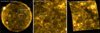 |
Fig. 1 AIA and HRIEUV images registered on 30 May, 2020 near 14:58 UTC. The panels show the real AIA 171 Å image (left), a zoomed-in view of the AIA region (middle), and the re-projected HRIEUV image (right). In the left panel, the zoomed-in view and the HRIEUV FOV are denoted by the outer white square and the color curve. The inner white square in the left panel and white squares in the middle and right panels denote the region used in the mutual DEM analysis. |
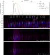 |
Fig. 2 Spectral responses of AIA 171 Å telescope and HRIEUV telescopes (top panel); the emission spectra calculated for different temperatures (second panel) and bottom two panels show the same spectra but multiplied with spectral responses of the telescopes. In the three bottom panels, the vertical coordinate corresponds to log T (see further explanations in the main text). |
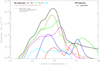 |
Fig. 3 Temperature response functions of AIA telescope (color curves) and HRIEUV telescope (black curve; see explanations in the main text). |
3 DEM calculation method and data preparation
For the DEM calculation, we used the method of Cheung et al. (2015), which is readily available in SolarSoft. The method assumes a piece-wise step function DEM(T), and instead of a differential DEM(T) as given by Eq. (2), it calculates the integrated emission measures at temperature bins Ti. Thus, Eq. (2) translates to3
 (3)
(3)
We used a temperature range with log Tmin = 5.6 (logarithm of K; thus, Tmin = 0.4 MK), Δ log T = 0.06, and 17 temperature bins, giving log Tmax = 6.62 (thus, Tmax = 4.2 MK). For the basis functions we used the default set of a delta function and two Gaussians with widths of 0.1 and 0.2 in log T. We also introduced GHRI(T) into the procedure.
We solved the system of either six, for the case of AIA only, or seven, for AIA and HRIEUV , equations given by Eq. (3) for every pixel in the image. The derivation of the DEM on the per-pixel basis, as compared to the per-structure basis, gives the advantage of eliminating a possible influence of different plasma conditions on the result. On the other hand, it poses stronger requirements on the precision of spatial co-alignment of the images, and their temporal correspondence. Since the AIA and the HRIEUV observe the solar corona from completely different vantage points, we re-projected the images from one vantage point to the other and interpolated the images to the same pixel grid. The re-projection/interpolation was done using the WCS routines4 (Thompson 2010, 2006) from SolarSoft. The transformations rely on the information from the headers of the FITS files, in particular from the position of the observer denoted by the DSUN_OBS, HGLN_OBS, HGLT_OBS, and other keywords; the projection information; the orientation; and the plate scale of the telescope denoted by WCSNAME, CRPIXj, CRVALj, and CRDELTj. Different directions of the re-projection can be used, either toward the HRIEUV or toward the AIA view. For the case where we only used the AIA data to calculate the DEM (Sect. 4), we calculated the DEM in the AIA pixel grid and calculated the simulated HRIEUV images. Only afterwards did we re-project them to the real HRIEUV pixel grid. For the mutual DEM analysis (Sect. 5), we re-projected the HRIEUV images to the AIA pixel grid from the very beginning and continued the analysis to the end. This choice was dictated by practical issues. In some cases, additional co-alignment of images was necessary, which we describe below.
It is worth noting that during the re-projection or re-scaling of the images, no change of the signal is required (i.e., there is no need to apply a factor 4 if the linear size of the image is doubled). This follows from the fact that the observed intensities Ij are treated in a way similar to brightness, that is, per unit area of the Sun, and the original Gj(T) functions were used.
The per-pixel analysis implies that all the images must be well co-aligned, such that the same pixel in different passbands corresponds to the same line-of-sight direction. Also, a good time-correlation is necessary. Because of a significantly closer distance to the Sun of the SolO, as compared to the Earth and the SDO, the same observational time expressed in UT and specified in the file names of both HRIEUV and AIA images corresponds to different moments on the Sun. Thus, for the HRIEUV we relied on the instant denoted by the EARTH_DATE keyword of the FITS headers and chose the images closest in time to the AIA images.
For the mutual DEM analysis, as described in Sect. 5, we reprojected the HRIEUV images to the vantage point and pixel grid of the AIA using the WCS routines from SolarSoft. In addition, we further reduced the region for the analysis to alleviate remaining misalignments between AIA and HRIEUV due to optical distortion across the FOV. We had to introduce additional shifts to the HRIEUV images by modifying their CRVAL header values by 5-10 arcsec, and we also introduced the additional shift of two pixels to the AIA 211 Å channel. Such transformations allowed us to obtain a good spatial correspondence of the images. Remaining displacement generally reduces the accuracy of the comparison, but since we rely on large areas of the FOV, it did not ruin our analysis.
An example of a crop from the AIA 171 Å, 193 Å, and 211 Å channels and the HRIEUV images taken on 30 May, 2020 is given in Fig. 4. Several crosses, the positions of which are the same in different images, annotate selected bright features.
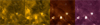 |
Fig. 4 Example of small crop pixels of AIA 171 Å, HRIEUV, 194, and 211 Å after a more precise co-alignment. |
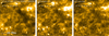 |
Fig. 5 Comparison of real HRIEUV image taken on 30 May, 2020 (left), simulated one calculated using DEM (middle), and AIA 171 Å image re-projected to HRIEUV pixel grid and re-normalized (right). The DEM was obtained using six channels - 94, 131, 171, 193, 211, and 335 Å - of the AIA telescope; then, the DEM was multiplied by GHRI(T). The resulting image was re-projected to the HRIEUV pixel grid, and finally the additional empirical coefficient k = 1.7 was used. For the AIA 171 Å, a coefficient k = 5.5 was used. An animated comparison is available online. |
4 DEM using AIA data only
In the first step, we calculated the DEM using only the AIA data, and then we simulated the HRIEUV image. We compared the real and the simulated images visually and using the histograms of the signals.
We show the results for the observations of 30 May, 2020, when the SolO was at the distance of 83.1 × 10⁶ km from the Sun (0.55 au) and the angular separation with the Earth was 31.3°. We calculated the DEM for a 1024 × 1024 pix FOV of the AIA that included the FOV of the HRIEUV , as denoted by the white square in Fig. 1, left panel. Then we convolved it with the GHRI(T), and finally re-projected the signal to the HRIEUV pixel grid. We found that the simulated image was dimmer than the real one; thus, we empirically found a coefficient of k = 1.7, such that the modified simulated image  matched the real one. The real and the simulated HRIEUV images are shown in Fig. 5 using the same color scale: the real one in the left panel, the modified-simulated image in the middle panel. In the right panel, we show an AIA 171 Å image re-projected to the HRIEUV pixel grid and re-normalized. The histograms of the signals are shown in Fig. 6.
The simulated image reproduces the real one with reasonable accuracy. The majority of the structures - a coronal hole in the central part, bright loops, and so on - are present in the simulated image and have reasonable brightnesses. The simulated image generally has higher contrast: many small regions with low intensity are present all over the FOV of the simulated image, while their counterparts in the real image have a larger signal (lower overall contrast). Such a difference can be caused by various factors, in particular differences in the thermal sensitivities of the HRIEUV and AIA, larger wings of the HRIEUV’s point spread function (PSF), and even projection effects. The reprojected AIA 171 Å image resembles the simulated one. The major difference between the two is observed inside and in proximity of the brightest loops, where the re-projected AIA 171 Å has less intensity. Since the two images - the simulated one and AIA 171 Å - are obtained from the AIA data, this difference in intensities can only be explained by the temperature effect: a combination of the temperature sensitivities of the 171 and 174 Å passbands and the temperature distribution of the real plasma.
The difference in intensities of bright loops can also be seen in the histograms, which for the case of the re-projected AIA 171 Å image has a steeper drop after the maximum.
There is a noticeably lower spatial resolution in the simulated image; while the angular size of the pixel is similar for the two instruments - 0.5 arcsec for HRIEUV and 0.6 arcsec for AIA - due to proximity to the Sun a single pixel in HRIEUV corresponds to 200 km, while in AIA it corresponds to 441 km. There is also an obvious displacement of the structures, which can be better seen when switching the images back and forth. It can be attributed to the greater heights of the structures in the solar atmosphere; during the re-projection step, a photospheric height is implicitly assumed. Such displacement should complicate direct comparison of the two images; however, since we compared them using histograms and relatively large FOV, we averaged the potential mismatch of individual pixels.
We repeated a similar comparison for the two other dates, when the separation between the two telescopes amounted to just a few degrees. There was a much better correspondence in the geometry of the simulated and the real HRIEUV images; however, as before we had to introduce an additional factor of k = 1.2 to match the intensities for 7 March, 2022. There was no need for a modification (i.e. k = 1) for 29 March, 2029. Examples of a real and a simulated image for 29 March, 2023 are given in Fig. 7.
The systematically lower intensity of all the pixels of the simulated HRIEUV images and the necessity to introduce k suggest the GHRI(T) of the HRIEUV is underestimated with respect to the AIA, for which periodic in-flight calibrations were performed. The temporal behavior - k = 1.7 coefficient in the beginning, k = 1.2 coefficient during 2022, and k = 1.0 during 2023 -might be explained by excessive sensitivity of the HRIEUV at the beginning of the mission and its gradual degradation by ~20% during the next two years. This degradation will be compatible with the degradation rate of other AIA channels (Boerner et al. 2014). The potential influence of the solar cycle and different plasma conditions must have a lesser impact on the results since the comparison is done for a large FOV that include various structures.
However, using the obtained DEMs we calculated simulated images for the AIA channels. We found a moderate mismatch of the intensities. The difference was already visible in the histograms; the histograms were either shifted to lower (171, 211 Å) or higher (193 Å channel) values. At the same time, the spatial structures in the simulated AIA images were reproduced with excellent accuracy. Thus, the observed discrepancies of the sim-ulated/real image intensities of HRIEUV might be partially caused by errors in the derived DEMs both in the case of AIA and HRIEUV.
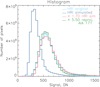 |
Fig. 6 Histograms of signal from Fig. 5: real HRIEUV image (light blue), a simulated one before k-normalization (dark blue), a k-normalized simulated image (red), and an AIA 171 Å image re-projected to the HRIEUV and re-normalized (green). |
5 DEM using HRIEUV and AIA data
In the next step, we calculated the DEM using both AIA and HRIEUV data. We chose the files representing the same time instant, re-projected the HRIEUV image to the AIA pixel grid, and ran the DEM-inversion procedure. As before, we considered additional cross-calibration factor k for the HRIEUV images; however, this time we divided the intensity of real HRIEUV images by k after the re-projection, but before the DEM-inversion. This actually corresponds fully to the previous approach. We tried various values of k ranging from k = 1.0 to k = 2.0. In order to improve the accuracy of the co-alignment and focus on the bright structures, we used a smaller FOV that only covered a portion of the HRIEUV FOV, for which the analysis was performed. We also checked that down-sampling of the images before DEMinversion to two- or four-times lower resolution does not modify the results.
5.1 30 May 2020
The context AIA 171 Å image taken at 14:58:45 UT is shown in Fig. 1 (left). The region over which the DEM was calculated is denoted by a white inner rectangle in the left panel panel, and the same regions are shown in middle and right panels. We reprojected the HRIEUV image to the AIA, divided it by k, and calculated the DEM.
In Fig. 8, we compare the real and the simulated images of six AIA channels and the HRIEUV telescope staying in the AIA pixel grid. A coefficient k = 1.6 was used to normalize the HRIEUV signal. Each panel is actually split into two parts along the diagonal, with the upper left part representing the simulated image and the bottom right part representing the real image (k-normalized in the case of HRIEUV). Each panel uses the same color scale for the simulated and the real data. Each simulated image corresponds to the real one with a good level of accuracy, such that the transition from the simulated to the real part can be inferred mostly from noise.
The histograms of the real and the simulated data also revealed a good correspondence. We show the results for 171, 193, and 211 Å channels of the AIA and the HRIEUV telescope below. The histograms of the real 94, 131, and 335 Å AIA images were significantly stretched by random noise (the average was matching the simulated data); thus, we do not show them. The influence of different k-coefficients on the simulated images is considered below in Fig. 9 and also in Appendix A. As before, each panel is split into two diagonally, showing the simulated and the real parts of the images. Below each panel, we provide the histograms of the signals.
With the cross-calibration factor k = 1.0, the DEM-inversion procedure failed to converge in many pixels. The situation improved significantly with an increase of k; however, at k = 1.2 (Fig. A.1) a large number of pixels still had no DEM solution and the histograms were mismatched. The cross-calibration factor k = 1.4 is presented in Fig. 9. According to the histograms, the simulated signal is on average lower than the real one by ~5-10 DN in the 193 Å and 211 Å channels. For the HRIEUV the simulated signal is slightly lower than the k-normalized real one. The transitions between the simulated and the real parts of the images are barely noticeable. The increase to k = 1.6 makes the correspondence slightly better for the HRIEUV, but slightly worse for the 171, 193, and 211 Å AIA channels (Fig. A.2; the image is visually similar to the one with k = 1.4).
The case with k = 1.8 is shown in Fig. A.3. The situation with the histograms’ correspondence starts to degrade, and the transition from the real to the simulated part of the images becomes more pronounced. With a further increase of the coefficient to k = 2.0, the correspondence degraded even more, as depicted in Fig. A.4. The black pixels (i.e., those for which a DEM-inversion procedure did not converge) started to appear, and the histograms for the simulated data deviated more from the real ones.
In order to quantify influence of different cross-calibration factors, we used 2D histograms, comparing the simulated and the real images (similarly to Vásquez et al. 2025). The results are presented in Fig. 10. The rows correspond to different crosscalibration factors, and the columns denote the channels. Each individual panel shows a 2D histogram of either simulated-versus-real or difference-versus-real intensities. In each histogram, the color encodes the number of occurrences in the given pair of images, the horizontal axis represents intensity of the real image, and the vertical axis represents the intensity of the simulated image or the difference (between the simulated and the real ones). For perfectly coinciding images, the simulated-versus-real histograms should be on a straight diagonal line, while for differences they should be on a horizontal line. The difference is used for the AIA 171, 193 Å, and HRI, since normal 2D histograms would be very close to a straight line (better than the AIA 211 Å). For the simulated-versus-real 2D histograms, the vertical scale corresponds to that of the horizontal axes. The Pearson correlation coefficient is shown in the top left of each panel.
The bottom row shows the situation with k = 1.0. The histograms for AIA 94, 211, and 335 Å are concentrated near the diagonal line; however, the 94 and 335 Å channels have significant spread. The simulated signal in 131 Å goes below the diagonal line, meaning lower signal in the simulated image. The 2D histograms for the 171, 193 Å, and the HRIEUV are concentrated near the horizontal line; however, in the case of 171 and 193 Å many pixels show greater intensity in the simulated images (above the horizontal line), and the HRIEUV show less intensity (below the horizontal line).
With the increase of the coefficient to k = 1.4 or k = 1.6, there is a significant improvement in symmetry for the 2D histograms for the 171, 193 Å and the HRIEUV, as well as improvement for the 131 Å channel occurs. We also see a significant improvement of the Pearson coefficients for all the channels. At the value k = 1.4 a transition occurs in the 171, 193 Å AIA, an HRIEUV histograms; the simulated signal of the 171 and 193 Å channels becomes smaller than the real one, while for the HRIEUV it becomes stronger than the real one. However, there is a clear improvement and shrinkage in spread for the 94, 131, 211, and 335 Å channels. Pearson coefficients become closer to unity. Any further increase of k degrades the correspondence.
As a result, we conclude that the intercalibration coefficient k = 1.4-1.6 gives much more consistent results during the DEMinversion procedure as compared to k = 1.0. This supports the value obtained in Sect. 4 for this date.
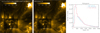 |
Fig. 7 Comparison of real HRIEUV image taken on 29 March, 2023 (left) and a simulated one (middle) calculated using DEM. The histograms are shown in the right panel. There was no need to introduce the additional cross-calibration factor k for this date. In the dark rectangle of the image, the signal was normalized by ×0.33 for visualization purposes. An animated comparison is available online. |
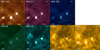 |
Fig. 8 Comparison of real and simulated images for six channels of AIA (3 left columns) and HRIEUV (bottom right panel) registered on 30 May, 2020. The DEM is obtained using simultaneous AIA and HRIEUV data. In the top row, the images represent 193 Å, 211 Å, and 335 Å channels (from left to right), and those in the bottom row represent the AIA 94 Å, 131 Å, and 171 Å channels and HRIEUV (from left to right). The FOV of these images is shown in Fig. 1. Each panel is actually split into two parts along the diagonal, showing the simulated image (top left part) and the real image (bottom right part). For the HRIEUV data, an additional cross-calibration factor k = 1.6 was introduced. |
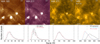 |
Fig. 9 Comparison of real and simulated images for AIA 193, 211, and 171 Å channels (from left to right, top row) and HRIEUV (top right panel) for the cross-calibration factor k = 1.4 for 30 May 2020. Each panel is split into two parts with the simulated part (top left) and the real part (bottom right) part. The FOV of these images is shown in Fig. 1. The plots under each panel show the histograms of the signal. |
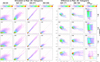 |
Fig. 10 Two-dimensional histograms of “simulated-versus-real” and “difference-versus-real” signals for different spectral channels of AIA and HRIEUV (annotated on top) for different cross-calibration values of k (annotated on the right) for observations on 30 May 2020. In each panel, the horizontal axis represents the intensity of the real image, the vertical axis represents the intensity of either the simulated image or the simulated-real difference, and the color encodes the number of occurrences in the given pair of images. For perfectly coinciding images, the simulated-versus-real signal should be a straight diagonal line, while for the difference-versus-real one it should be a horizontal line. |
 |
Fig. 11 AIA 171 Å channel image registered on 7 March 2022. The HRIEUV FOV is denoted by a color rectangle. The white square denotes the region used for mutual DEM analysis. |
5.2 7 March, 2022
We performed a similar analysis for the observations performed on 7 March 2022, when the angular separation was 3.0°. A fullSun AIA 171 Å image is given in Fig. 11, where the FOV of the HRIEUV is denoted by a colored square and the region chosen for the mutual DEM analysis is shown by white square. All the processing steps - spatial and temporal co-alignment - were repeated with corresponding parameters. Analysis of the histograms suggested the best value k = 1.4. A comparison of the real and the simulated images and their histograms is given in Fig. 12.
The 2D histograms are given in Fig. B.1. The value k = 1.0 clearly shows poor correspondence of the simulated and real signals, in particular in the 131, 171, and 193 Å AIA channels and HRIEUV . For higher k values, the 2D histograms show a much better correspondence for the other three values: k = 1.2, k = 1.4, and k = 1.6. Pearson coefficients show a maximum either for k = 1.4 or k = 1.6, depending on the channel. In the simulated images, k = 1.2 gives slightly more black pixels, for which the DEM-inversion procedure did not converge. With a further increase of k above 1.6, the correspondence starts to degrade. Thus, we conclude that the cross-calibration factor on the order of k = 1.4-1.6 should be used. This value is slightly larger than that obtained in Sect. 4 for this date.
5.3 29 March, 2023
On 29 March 2023 the angular separation of AIA and EUI was 2.8°. A full-Sun AIA 171 Å image taken at 12:45 UT is given in Fig. 13. The FOV of the HRIEUV is denoted by the colored square, and the region chosen for the mutual DEM analysis is shown by white square.
As before, we applied the necessary processing steps and calculated the DEM using six AIA images and the HRIEUV images, and we calculated the simulated images. In Fig. 14, we compare the real and simulated images for k = 1.4. Each panel is split into two parts with the real and the simulated data over the diagonal line. The simulated images correspond to the real counterparts with a good level of accuracy. The top right panel shows a zoomed-in view of a small region with bright loops, which we will analyze in the following section.
The 2D histograms are given in Fig. C.1. For the values k = 1.2, 1.4, and 1.6, the 2D histograms are quite similar; however, Person coefficients are highest for k = 1.4. At k = 1.0 or k > 1.6, the correspondence degrades. Thus, we conclude the cross-calibration factor k = 1.4 should be used. This value of k is significantly higher than the one obtained in Sect. 4 for this date.
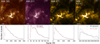 |
Fig. 12 Comparison of real and simulated images for the AIA 193, 211, and 171 Å channels (from left to right, top row) and HRIEUV (top right panel) for the cross-calibration factor k = 1.4 for the observations on 7 March 2022. The FOV of these images is shown in Fig. 11. See also annotation for Fig. 9. |
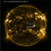 |
Fig. 13 AIA 171 Å channel image registered on 29 March 2023. The FOV of the HRIEUV is denoted by a color rectangle, and the white square denotes the region used for mutual DEM analysis. |
6 Discussion and conclusions
In most of the cases considered in Sects. 4 and 5, we find that the discrepancies of the GHRI (T) and those of the AIA telescope are on the order of 40%, meaning that in the real HRIEUV images the signal is ~40% higher than those derived from the AIA data. Given the complexity and long chain of conversions necessary to calculate G(T) for an arbitrary telescope, this level of correspondence of the absolute calibrations of the two telescopes can be considered as very good. On the other hand, this discrepancy should be taken into account if the DEM (or DEM-like) analysis is performed using simultaneous observations. In general, errors in a Gj(T) function can be separated into two classes: an error of its peak value, and an error in its shape. The first type of errors can be attributed to underestimated optical throughput of a telescope, which can be due to, for example, unaccounted shadowing by filter meshes or the uncertainty of the degradation. The second type can be attributed to moderate accuracy of the emission spectrum model (e.g., not all spectral lines are present) or errors in the spectral throughput of the telescope. As mentioned in Sect. 2, our GHRI(T) takes into account all the known factors, including the Gj(T) of AIA, which is also based on the very detailed models. For the AIA, we relied on the degradation provided by the aia_bp_get_corrections.pro routine from the SolarSoft during a private discussion with AIA scientists (M. Jin and W. Liu); they confirmed the adequacy of these data. The errors of the second type are more difficult to reveal, as the real spectroscopic observations are needed. For example, simultaneous observations of the AIA telescope and the EVE spectrograph on board SDO allowed Boerner et al. (2014) to make such a conclusion and update temperature sensitivities of the 94 and 131 Å channels of the AIA telescope. However, in the case of HRIEUV the main spectral region near 171 Å is well studied, and problems with the atomic data are less likely.
A 2D map of EMTi calculated using seven channels - the HRIEUV and six AIA channels - for 29 March 2023 is presented in Fig. 15. The temperature bin of each panel is denoted in the bottom left part. In the third column, we denote masks of three bright loops, which we have chosen for the analysis. The obtained EM map corresponds to the typically assumed model: the majority of the quiet-Sun plasma has a temperature in the 1.0-2.5 MK (log T ∊ [6.0,6.4]) range. At the same time, the bright loops have higher EM with respect to the surrounding corona in all temperature bins. The enhanced EM must be interpreted as the presence of plasma with higher density. In addition, the bright loops contain plasma with T > 2.3 MK (log T > 6.35), which is almost absent in quiet-Sun regions.
A similar EM map calculated using only six AIA channels was actually very similar, and it was not easy to see any differences via visual inspection. That is why we compared DEM(T) profiles of several bright loops, which are annotated in Figs. 14 and 15. We created masks to isolate the loops, measured the average signal within the masks, and calculated the DEM(T) using the signals both with and without the HRIEUV data. We show the measured DEM(T) in Fig. 16. The solid lines represent seven channels’ DEMs, while dash-dotted lines represent only six AIA channels. The three panels correspond to loop 2, loop 3, and loop 4. Loop 2 has enhanced EM at temperatures from 1.32.3 MK (log T ∊ [6.11, 6.35]); however, at higher temperatures its EM drops. The two other loops have a peak temperature of 2.5 MK, an EM similar to that of hotter plasma, and a slight dip at 0.6-1.0 MK. The DEMs calculated with and without the HRIEUV for the three loops have many similarities; introducing the HRIEUV data into the DEM-inversion procedure mainly modifies the EM of worm plasma with T ~ 1 MK.
Since the spectral and temperature responses of the AIA 171 Å channel and the HRIEUV are sufficiently close, the reprojected AIA 171 Å image resembles the HRIEUV quite well. However, as is shown in Fig. 5 and during discussion of the DEM analysis, adding the HRIEUV signal to the DEM-inversion procedure does change the results. Thus, using of HRIEUV data is desirable not only to achieve higher spatial resolution, but also to better understand the processes in the emitting plasma.
The DEM-inversion procedure is known to be error-prone (Judge et al. 1997; Guennou et al. 2012). In addition to the ill-posed nature of the inverse problem and influence of noise in the measured data, there are other sources that enhance the possibility of errors. These are potential errors in the atomic data, errors in spectral sensitivities of the telescopes, inapplicability of the assumptions such as abundances, ionization, and equilibrium. We note, however, that in the current analysis we use the derived DEMs not to infer the properties of the emitting plasma, but rather to compute the signal in different passbands. This reduces the possible impact of errors related to the assumptions (all the spectral channels will be influenced in a similar way) and the spectral sensitivities of the telescopes. Furthermore, since in our method we compare the signals within a large FOV, which includes different plasma structures, this further reduces the influence of applicability of the assumptions, dependence on plasma temperature, and so on.
However, we verified that changes in the parameters of the DEM inversion procedure, such as the variation of Tmin, do not change the results. We also tried the older versions of the temperature sensitivities of the telescopes, which were calculated with the same spectral sensitivities of the telescopes, but with a different spectral model (sun_coronal_1992_feldman_ext abundances were), and it did not change the results significantly. A comparison of older and newer temperature responses is given in Appendix D.
The k coefficient determined in Sect. 5 had values of 1.6, 1.4, and 1.4 for the periods May 2020, March 2022, and March 2023. The slight decrease could be interpreted as a gradual degradation of the HRIEUV telescope. In order to verify the hypothesis, we compared correspondence of the HRIeuv and 171 Å AIA channel signals for 21 dates from 2020-2023. These dates were chosen irregularly due to the SolO observation schedule. However, the uncertainties of the method such as varying solar activity, presence of active regions, different vantage points, did not allow us to make a firm conclusions.
Our approach, which is based on a comparison of the real and the simulated signal over large areas, gives some advantages over traditional ones, which consider single structure or average across some region. It can be used as a strategy for intercalibration of all contemporary EUV imagers (also EUVI, SWAP, SUVI, and EIT). A golden reference across solar cycles and EUV instruments, similar perhaps to the intercalibration or total solar irradiance (TSI) radiometers, would be ideal.
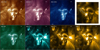 |
Fig. 14 Similar to Fig. 8, but for 29 March 2023. The FOV of these images is shown in Fig. 13. A cross-calibration factor k = 1.4 was used. The top right panel shows a zoomed-in view of the region of the HRIEUV signal with annotated several bright loops. |
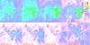 |
Fig. 15 Two-dimensional map of emission measure EMTi in different temperature bins for 29 March 2023, calculated for k = 1.4. The temperature bin of each panel is annotated in the lower left corner. In the panels of the third column, several loops are annotated and were analyzed in detail. |
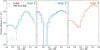 |
Fig. 16 Comparison of DEM(T) calculated using either six AIA channels or HRIEUV and six AIA channels for several bright loops. For the case of a mutual HRIEUV and AIA analysis, the coefficient k = 1.4 was used. |
Data availability
Movies associated to Fig. 5 and 7 are available at https://www.aanda.org
Movies
Movie associated to Fig 5 and 7 Access Supplementary Material
Movie associated to Fig 5 and 7 Access Supplementary Material
Acknowledgements
Solar Orbiter is a space mission of international collaboration between ESA and NASA, operated by ESA. The EUI instrument was built by CSL, IAS, MPS, MSSL/UCL, PMOD/WRC, ROB, and LCF/IO with funding from the Belgian Federal Science Policy Office (BELSPO/PRODEX PEA 4000106864 and 4000112292); the Centre National d’Etudes Spatiales (CNES); the UK Space Agency (UKSA); the Bundesministerium fuür Wirtschaft und Energie (BMWi) through the Deutsches Zentrum fuür Luft- und Raumfahrt (DLR); and the Swiss Space Office (SSO). SS acknowledges the Belgian FEDtWIN program. SS is also grateful to Abderraouf Yamani for his support. The research that led to these results was subsidized by the Belgian Federal Science Policy Office through the contract B2/223/P1/CLOSE-UP. A.N.Z. thanks the Belgian Federal Science Policy Office (BELSPO) for the provision of financial support in the framework of the PRODEX Programme of the European Space Agency (ESA) under contract Nos. 4000136424 and 4000143743.
Appendix A Additional images for 30 May 2020
Comparison of the real and the simulated images for k = 1.2, k = 1.6, k = 1.8, and k = 2.0 are presented in Figs. A.1–A.4. for the observations on 30 May 2020.
Appendix B 2D histograms for 07 March 2022
Two-dimensional histograms for 07 March 2022 are presented in Fig. B.1.
Appendix C 2D histograms for 29 March 2023
Two-dimensional histograms for 29 March 2023 are presented in Fig. C.1.
Appendix D Comparison of old and new temperature responses
In Fig. D.1 we compare the older (called model 2022; dashed curves) and the most recent (called model 2024; solid curves) temperature responses calculated by us and provided in SolarSoft via the aia_get_response(/temp) (dotted curves). For the curves provided in SolarSoft degradation factors and NH/Ne = 0.83 were used. The temperature responses, calculated by us relied on different abundances - sun_coronal_1992_feldman_ext in the 2022 model, sun_coronal_2021_chianti in the 2024 model - of CHIANTI v10. Also in the 2024 model the HRIEUV spectral sensitivity was updated. The 2022 model corresponds well with the data provided by SolarSoft.
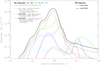 |
Fig. D.1 Analysis of influence of spectral model on the temperature response functions. The color curves represent the AIA telescope, and the black curves represent the HRIEUV telescope. The dashed and dotted curve correspond to the older spectral model. See details in text. |
References
- Berghmans, D., Auchère, F., Long, D. M., et al. 2021, A&A, 656, L4 [NASA ADS] [CrossRef] [EDP Sciences] [Google Scholar]
- Boerner, P., Edwards, C., Lemen, J., et al. 2012, Sol. Phys., 275, 41 [Google Scholar]
- Boerner, P. F., Testa, P., Warren, H., Weber, M. A., & Schrijver, C. J. 2014, Sol. Phys., 289, 2377 [Google Scholar]
- Cheung, M. C., Boerner, P., Schrijver, C. J., et al. 2015, ApJ, 807, 143 [Google Scholar]
- Chitta, L. P., Zhukov, A. N., Berghmans, D., et al. 2023, Science, 381, 867 [NASA ADS] [CrossRef] [Google Scholar]
- Culhane, J. L., Harra, L. K., James, A. M., et al. 2007, Sol. Phys., 243, 19 [Google Scholar]
- Del Zanna, G., Dere, K. P., Young, P. R., & Landi, E. 2021, ApJ, 909, 38 [NASA ADS] [CrossRef] [Google Scholar]
- Delaboudinière, J. P., Artzner, G. E., Brunaud, J., et al. 1995, Solar Phys., 162, 291 [Google Scholar]
- Dere, K., Landi, E., Mason, H., Fossi, B. M., & Young, P. 1997, A&AS, 125, 149 [NASA ADS] [CrossRef] [EDP Sciences] [Google Scholar]
- Freeland, S. L., & Handy, B. N. 1998, Sol. Phys., 182, 497 [Google Scholar]
- Gissot, S., Auchère, F., Berghmans, D., et al. 2023, A&A, in press [arXiv:2307.14182] [Google Scholar]
- Guennou, C., Auchère, F., Soubrié, E., et al. 2012, ApJS, 203, 25 [NASA ADS] [CrossRef] [Google Scholar]
- Hock, R. A., & Eparvier, F. G. 2008, Solar Phys., 250, 207 [Google Scholar]
- Howard, R. A., Moses, J. D., Vourlidas, A., et al. 2008, Space Sci. Rev., 136, 67 [NASA ADS] [CrossRef] [Google Scholar]
- Judge, P. G., Hubeny, V., & Brown, J. C. 1997, ApJ, 475, 275 [NASA ADS] [CrossRef] [Google Scholar]
- Kraaikamp, E., Gissot, S., Stegen, K., et al. 2023, SolO/EUI Data Release 6.0 2023-01, https://doi.org/10.24414/z818-4163 (Royal Observatory of Belgium (ROB)) [Google Scholar]
- Lemen, J. R., Title, A. M., Akin, D. J., et al. 2012, Sol. Phys., 275, 17 [Google Scholar]
- Pesnell, W. D., Thompson, B. J., & Chamberlin, P. C. 2012, Sol. Phys., 275, 3 [Google Scholar]
- Petrova, E., Van Doorsselaere, T., Berghmans, D., et al. 2024, A&A, 687, A13 [NASA ADS] [CrossRef] [EDP Sciences] [Google Scholar]
- Pottasch, S. R. 1964, Space Sci. Rev., 3, 816 [NASA ADS] [CrossRef] [Google Scholar]
- Raftery, C. L., Bloomfield, D. S., Gallagher, P. T., et al. 2013, Sol. Phys., 286, 111 [Google Scholar]
- Rochus, P., Auchère, F., Berghmans, D., et al. 2020, A&A, 642, A8 [NASA ADS] [CrossRef] [EDP Sciences] [Google Scholar]
- Seaton, D. B., Berghmans, D., Nicula, B., et al. 2013, Sol. Phys., 286, 43 [NASA ADS] [CrossRef] [Google Scholar]
- Shestov, S., Reva, A., & Kuzin, S. 2014, ApJ, 780, 15 [Google Scholar]
- Shrivastav, A. K., Pant, V., Berghmans, D., et al. 2024, A&A, 685, A36 [NASA ADS] [CrossRef] [EDP Sciences] [Google Scholar]
- Thompson, W. 2010, The SolarSoft WCS Routines: A Tutorial, NASA Goddard Space Flight Center, Adnet Systems, Inc. [Google Scholar]
- Thompson, W. T. 2006, A&A, 449, 791 [NASA ADS] [CrossRef] [EDP Sciences] [Google Scholar]
- Vásquez, A. M., Nuevo, F. A., Burtovoi, A., et al. 2025, Sol. Phys., 300, 4 [Google Scholar]
- Woods, T. N., Eparvier, F. G., Hock, R., et al. 2012, Sol. Phys., 275, 115 [Google Scholar]
- Zhukov, A. N., Mierla, M., Auchère, F., et al. 2021, A&A, 656, A35 [NASA ADS] [CrossRef] [EDP Sciences] [Google Scholar]
DOI: 10.24414/z818-4163
M. Jin and W. Liu from the AIA team confirmed validity of the data in a private discussion.
While we keep using the phrase “DEM analysis”.
All Figures
|
Fig. 1 AIA and HRIEUV images registered on 30 May, 2020 near 14:58 UTC. The panels show the real AIA 171 Å image (left), a zoomed-in view of the AIA region (middle), and the re-projected HRIEUV image (right). In the left panel, the zoomed-in view and the HRIEUV FOV are denoted by the outer white square and the color curve. The inner white square in the left panel and white squares in the middle and right panels denote the region used in the mutual DEM analysis. |
| In the text | |
|
Fig. 2 Spectral responses of AIA 171 Å telescope and HRIEUV telescopes (top panel); the emission spectra calculated for different temperatures (second panel) and bottom two panels show the same spectra but multiplied with spectral responses of the telescopes. In the three bottom panels, the vertical coordinate corresponds to log T (see further explanations in the main text). |
| In the text | |
|
Fig. 3 Temperature response functions of AIA telescope (color curves) and HRIEUV telescope (black curve; see explanations in the main text). |
| In the text | |
|
Fig. 4 Example of small crop pixels of AIA 171 Å, HRIEUV, 194, and 211 Å after a more precise co-alignment. |
| In the text | |
|
Fig. 5 Comparison of real HRIEUV image taken on 30 May, 2020 (left), simulated one calculated using DEM (middle), and AIA 171 Å image re-projected to HRIEUV pixel grid and re-normalized (right). The DEM was obtained using six channels - 94, 131, 171, 193, 211, and 335 Å - of the AIA telescope; then, the DEM was multiplied by GHRI(T). The resulting image was re-projected to the HRIEUV pixel grid, and finally the additional empirical coefficient k = 1.7 was used. For the AIA 171 Å, a coefficient k = 5.5 was used. An animated comparison is available online. |
| In the text | |
|
Fig. 6 Histograms of signal from Fig. 5: real HRIEUV image (light blue), a simulated one before k-normalization (dark blue), a k-normalized simulated image (red), and an AIA 171 Å image re-projected to the HRIEUV and re-normalized (green). |
| In the text | |
|
Fig. 7 Comparison of real HRIEUV image taken on 29 March, 2023 (left) and a simulated one (middle) calculated using DEM. The histograms are shown in the right panel. There was no need to introduce the additional cross-calibration factor k for this date. In the dark rectangle of the image, the signal was normalized by ×0.33 for visualization purposes. An animated comparison is available online. |
| In the text | |
|
Fig. 8 Comparison of real and simulated images for six channels of AIA (3 left columns) and HRIEUV (bottom right panel) registered on 30 May, 2020. The DEM is obtained using simultaneous AIA and HRIEUV data. In the top row, the images represent 193 Å, 211 Å, and 335 Å channels (from left to right), and those in the bottom row represent the AIA 94 Å, 131 Å, and 171 Å channels and HRIEUV (from left to right). The FOV of these images is shown in Fig. 1. Each panel is actually split into two parts along the diagonal, showing the simulated image (top left part) and the real image (bottom right part). For the HRIEUV data, an additional cross-calibration factor k = 1.6 was introduced. |
| In the text | |
|
Fig. 9 Comparison of real and simulated images for AIA 193, 211, and 171 Å channels (from left to right, top row) and HRIEUV (top right panel) for the cross-calibration factor k = 1.4 for 30 May 2020. Each panel is split into two parts with the simulated part (top left) and the real part (bottom right) part. The FOV of these images is shown in Fig. 1. The plots under each panel show the histograms of the signal. |
| In the text | |
|
Fig. 10 Two-dimensional histograms of “simulated-versus-real” and “difference-versus-real” signals for different spectral channels of AIA and HRIEUV (annotated on top) for different cross-calibration values of k (annotated on the right) for observations on 30 May 2020. In each panel, the horizontal axis represents the intensity of the real image, the vertical axis represents the intensity of either the simulated image or the simulated-real difference, and the color encodes the number of occurrences in the given pair of images. For perfectly coinciding images, the simulated-versus-real signal should be a straight diagonal line, while for the difference-versus-real one it should be a horizontal line. |
| In the text | |
|
Fig. 11 AIA 171 Å channel image registered on 7 March 2022. The HRIEUV FOV is denoted by a color rectangle. The white square denotes the region used for mutual DEM analysis. |
| In the text | |
|
Fig. 12 Comparison of real and simulated images for the AIA 193, 211, and 171 Å channels (from left to right, top row) and HRIEUV (top right panel) for the cross-calibration factor k = 1.4 for the observations on 7 March 2022. The FOV of these images is shown in Fig. 11. See also annotation for Fig. 9. |
| In the text | |
|
Fig. 13 AIA 171 Å channel image registered on 29 March 2023. The FOV of the HRIEUV is denoted by a color rectangle, and the white square denotes the region used for mutual DEM analysis. |
| In the text | |
|
Fig. 14 Similar to Fig. 8, but for 29 March 2023. The FOV of these images is shown in Fig. 13. A cross-calibration factor k = 1.4 was used. The top right panel shows a zoomed-in view of the region of the HRIEUV signal with annotated several bright loops. |
| In the text | |
|
Fig. 15 Two-dimensional map of emission measure EMTi in different temperature bins for 29 March 2023, calculated for k = 1.4. The temperature bin of each panel is annotated in the lower left corner. In the panels of the third column, several loops are annotated and were analyzed in detail. |
| In the text | |
|
Fig. 16 Comparison of DEM(T) calculated using either six AIA channels or HRIEUV and six AIA channels for several bright loops. For the case of a mutual HRIEUV and AIA analysis, the coefficient k = 1.4 was used. |
| In the text | |
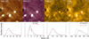 |
Fig. A.1 Same as in Fig. 9, but for k = 1.2. |
| In the text | |
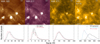 |
Fig. A.2 Same as in Fig. 9, but for k = 1.6. |
| In the text | |
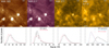 |
Fig. A.3 Same as in Fig. 9, but for k = 1.8. |
| In the text | |
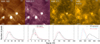 |
Fig. A.4 Same as in Fig. 9, but for k = 2.0. |
| In the text | |
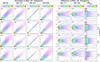 |
Fig. B.1 Similar to Fig. 10, but for the 7 March 2022. |
| In the text | |
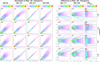 |
Fig. C.1 Similar to Fig. 10, but for the 29 March 2023. |
| In the text | |
|
Fig. D.1 Analysis of influence of spectral model on the temperature response functions. The color curves represent the AIA telescope, and the black curves represent the HRIEUV telescope. The dashed and dotted curve correspond to the older spectral model. See details in text. |
| In the text | |
Current usage metrics show cumulative count of Article Views (full-text article views including HTML views, PDF and ePub downloads, according to the available data) and Abstracts Views on Vision4Press platform.
Data correspond to usage on the plateform after 2015. The current usage metrics is available 48-96 hours after online publication and is updated daily on week days.
Initial download of the metrics may take a while.