| Issue |
A&A
Volume 699, July 2025
|
|
|---|---|---|
| Article Number | A315 | |
| Number of page(s) | 14 | |
| Section | Galactic structure, stellar clusters and populations | |
| DOI | https://doi.org/10.1051/0004-6361/202450867 | |
| Published online | 17 July 2025 | |
The Sagittarius stellar stream embedded in a fermionic dark matter halo
1
Instituto de Astrofísica de La Plata (CONICET-UNLP),
Paseo del Bosque S/N,
La Plata 1900, Buenos Aires,
Argentina
2
Facultad de Ciencias Astronómicas y Geofísicas de La Plata (UNLP),
Paseo del Bosque S/N,
La Plata 1900, Buenos Aires,
Argentina
3
ICRANet,
Piazza della Repubblica 10,
65122 Pescara,
Italy
* Corresponding author: This email address is being protected from spambots. You need JavaScript enabled to view it.
Received:
24
May
2024
Accepted:
14
May
2025
Abstract
Context. Stellar streams are essential tracers of the gravitational potential of the Milky Way, with key implications for the problem of dark matter model distributions, either within or beyond phenomenological ΛCDM halos.
Aims. For the first time in the literature, a dark matter (DM) halo model based on first physical principles such as (quantum) statistical mechanics and thermodynamics is used to try to reproduce the 6D observations of the Sagittarius (Sgr) stream. Thus, we aim to extract quantitative and qualitative conclusions on how well our assumptions stand with respect to the observations. We model both DM halos, the one of the Sgr dwarf and the one of its host, with a spherical self-gravitating system of neutral fermions that accounts for the effects of particle escape and fermion degeneracy (due to the Pauli exclusion principle), the latter causing a high-density core at the center of the halo. Full baryonic components for each galaxy are also considered.
Methods. We used a spray algorithm with ∼ 105 particles to generate the Sgr tidal debris, which evolves in the combined gravitational potential of the host-progenitor system, to then make a direct comparison with the full phase-space data of the stream. We repeated this kind of simulation for different parameter setups of the fermionic model including the particle mass, with special attention to testing different DM halo morphologies allowed by the physics, including polytropic density tails as well as power-law-like trends.
Results. We find that the fermionic halo models considered can only reproduce the trailing arm of the Sgr stream. Within the observationally allowed span of enclosed masses where the stream moves, neither the power-law-like nor the polytropic behavior of the fermionic halo models can answer for the observed trend of the leading tail – a conclusion that is shared by former analyses using other types of spherically symmetric halos. Thus, we conclude that further model improvements, such as abandoning spherical symmetry and including the Large Magellanic Cloud perturber, are needed for the proper modeling of the overall Milky Way potential within this kind of first-principle halo model.
Key words: Galaxy: halo / Galaxy: kinematics and dynamics / dark matter
© The Authors 2025
 Open Access article, published by EDP Sciences, under the terms of the Creative Commons Attribution License (https://creativecommons.org/licenses/by/4.0), which permits unrestricted use, distribution, and reproduction in any medium, provided the original work is properly cited.
This article is published in open access under the Subscribe to Open model. This email address is being protected from spambots. You need JavaScript enabled to view it. to support open access publication.
1 Introduction
Stellar streams are important tracers of the gravitational potential of the Galaxy, extending from the innermost to outermost radial extents, and thus allow one to infer the mass distribution of the host (see e.g. Li et al. 2019; Mateu 2023; Ibata et al. 2024; Bonaca & Price-Whelan 2024, for the current state of tidal debris in the Milky Way). The information content on the gravitational potential of the Milky Way (MW) provided by cold stellar streams, such as the iconic GD-1 (Grillmair & Dionatos 2006), was theoretically studied by Bonaca & Hogg (2018). Among a series of interesting results, they found that in simple analytic models of the MW, streams in eccentric orbits are better at constraining the halo shape. Generally, for each single stream they find degeneracies between the properties of the dark matter (DM) halo and the baryonic potentials. They show that a simultaneous fit of multiple streams will constrain all parameters at the percent level using basis function expansions to give the gravitational potential more freedom.
Within the vast spectra of tidal stream properties, there exist in the MW examples of long stellar streams such as the Orphan-Chenab and the Sagittarius streams. Their currently measured angles subtended in the sky are 210° (Koposov et al. 2019) and more than 360° (Majewski et al. 2003; Ibata et al. 2020), respectively. The former stream has a width of ∼2°, being rather thin in spite of having an unknown massive progenitor (Hawkins et al. 2023; Belokurov et al. 2007). In this work, we study the latter stream, which was tidally built from the Sgr dwarf progenitor. It is the most extended in length and width of all the MW streams observed to date, and it is possible to get crucial information from it about the DM halo potential and morphology (Ibata et al. 2001; Helmi 2004; Law et al. 2005; Johnston et al. 2005; Law et al. 2009; Law & Majewski 2010; Deg & Widrow 2013; Vasiliev et al. 2021).
The first observations of the Sgr stream progenitor were performed by Ibata et al. (1994). After that, a big effort was made to determine the remnant structures arising from this progenitor (e.g., Totten & Irwin 1998; Mateo et al. 1998; Majewski et al. 1999; Dinescu et al. 2002; Newberg et al. 2002, 2003, 2007; Yanny et al. 2009; Koposov et al. 2012; Koposov et al. 2013; Slater et al. 2013; Huxor & Grebel 2015; Luque et al. 2017; Hernitschek et al. 2017; Antoja et al. 2020; Ramos et al. 2020; Ibata et al. 2020). The first global spatial characterization of the stellar stream stripped from Sagittarius was obtained by Majewski et al. (2003) with the Two Micron All Sky Survey (2MASS) using M giant star data. In these observations, it was concluded that the tidal debris left by this satellite develops two tails: the leading one spreading along the northern Galactic hemisphere, and the trailing one lying in the southern part of it. Afterward, Majewski et al. (2004) performed radial velocity measurements, enabling subsequent dynamical modeling of the stream (Law et al. 2005).
The structure and evolution of the Sgr dwarf stream, together with the overall gravitational potential of the host Galaxy, are still open, coupled problems because there is not yet a single full model able to fit the astrometric, photometric, and spectrometric observations performed to date. Successful enough examples in that direction were produced by Law & Majewski (2010) through N–body simulations, modeling the tidal disruption suffered by the Sgr dwarf on its way around the MW. For that purpose, they fit radial velocity data of a sample of 2MASS M-giants in combination with SDSS photometry. Similar results were obtained in Deg & Widrow (2013), in which a Bayesian analysis was performed using single-particle orbits to model the MW potential. In Gibbons et al. (2014), the predicted Sgr tidal stream was used to measure the cumulative mass of the Galaxy based on the values of the apocentric distances of the arms and the precession angle of the stream (Belokurov et al. 2014). In Fardal et al. (2019), they tested their kinematics and spatial predictions for Sgr tidal debris with RR Lyrae observations from Pan-STARRS1, paying special attention to the apocenter distances of the stream. The work of Dierickx & Loeb (2017) has provided proof of the main features of the Sgr stream using mock tidal debris computed with GADGET (Springel 2005). Further improvements in the stream N-body model have also been made by Wang et al. (2022) with a spherical DM halo and by Vasiliev et al. (2021) through the inclusion of the Large Magellanic Cloud (LMC). The latter model constitutes the paradigm that agrees best with current observations of the Sgr stream.
Despite the reliability of the numerical simulations, it is necessary to improve the long computation times and to try semi-analytical methods in order to be more flexible in studying different DM halo models and their associated free parameter space. This can be achieved by the use of ejection algorithms (sometimes called spray methods), such as the ones implemented in Varghese et al. (2011), Küpper et al. (2012), Gibbons et al. (2014), Bowden et al. (2015), and Fardal et al. (2015). The methodology of these algorithms consists of the ejection of stars with adequate initial conditions at the two Lagrange points around the progenitor, to then integrate them over a long enough time span and get the orbit of all the stars. As was demonstrated in Gibbons et al. (2014), in order for this semi-analytical method to be almost indistinguishable from the simulations, it is necessary to include the action of the gravity of the progenitor in addition to that of the host.
Most studies aiming to reproduce the Sgr stream were developed under the assumption of phenomenological DM halo profiles. For instance, by using different axisymmetric halo potentials such as prolate or oblate logarithmic functions (Johnston et al. 2005; Law et al. 2005), by applying axisymmetric variations of traditional ΛCDM halos (Law et al. 2005), or by employing very specific realizations of triaxial halos (Law & Majewski 2010)1. Perhaps the most notorious example is the DM halo model suggested by (Vasiliev et al. 2021), in which they considered a complex halo whose axis ratios and principal axis orientations vary with radius. Their best-fit model has two effective components, one rotated with respect to the other, in addition to the perturbative effects of the LMC. However, the use of such purely phenomenological DM profiles is impractical for obtaining information about the underlying DM nature, particle mass, and cosmological framework. An interesting though poorly investigated alternative is to study stellar streams via numerical methods that incorporate DM halo potentials obtained from first-principle physics. Such models are based on statistical mechanics and thermodynamics, in which the quantum nature of the DM particles is included. This has been studied in Robles et al. (2015) for bosonic DM particles, in which the DM halo is modeled via a self-gravitating system of self-interacting scalar-field dark matter (SFDM), which forms a Bose-Einstein condensate. However, that work was only applied to hypothetical (or generic) dwarf satellites hosted by a MW-like galaxy, and mainly focused on comparing the tidal effects with respect to CDM halos.
Recently, Mestre et al. (2024) have modeled the GD-1 5D track with a MW that includes a fermionic DM halo model built from first principles, such as the Ruffini–Argüelles–Rueda (RAR) model (see Ruffini et al. 2015; Argüelles et al. 2018 for the original works, and Argüelles et al. 2023a for a review). The RAR model is built in terms of a self-gravitating system of massive fermions at a finite temperature, whose more general solutions can include two different regimes in the same system: one to be highly degenerate at the center, forming a dense fermion core (thanks to the Pauli exclusion principle), and one diluted in the halo region (resembling the King pro-file). The successful phenomenological analysis of this model has recently been shown for different galaxy types and scaling relations (Argüelles et al. 2019; Krut et al. 2023), including our own Galaxy (Argüelles et al. 2018; Becerra-Vergara et al. 2020, 2021; Argüelles et al. 2022; Argüelles & Collazo 2023). In the latter case, we showed that the central DM core can work as an alternative to the massive black hole (BH) in SgrA*, while the outer halo explains the Galaxy rotation curve.
Important aspects of this kind of first-principle physics model (for bosonic or fermionic DM) with respect to the ones arising from classical N-body simulations are that the resulting density profiles have a cored2 nature at inner halo scales (i.e., not cuspy as in CDM-only cosmologies), and that they depend on the particle mass (see e.g., Chavanis et al. 2015; Argüelles et al. 2021 for the fermionic case). Another relevant advantage of this kind of astrophysical core–halo fermionic DM profile is that one can apply thermodynamical tools and demonstrate that these distributions remain stable during cosmological timescales once formed (Argüelles et al. 2021). Also, one can show that there exists a critical fermion core mass above which the core collapses toward a supermassive black hole (SMBH), with important applications to the high-redshift Universe (Argüelles et al. 2023b, 2024).
Thus, in this work we aim to reproduce, for the first time in the literature, the main features of the Sgr stellar stream observations, assuming that both the DM halo of our Galaxy and the one of the Sgr dwarf are composed of fermionic DM halos according to the RAR model Argüelles et al. (2018). For such an endeavor, we apply the ejection method proposed in Gibbons et al. (2014), and thus we consider the self-gravity caused by the satellite. This allows us to explore a considerable range of free parameters of the DM models in manageable computing times, paying special attention to testing different DM halo tails allowed by the physics of the fermionic model.
The flow of the work is as follows. In Sect. 2, we detail the data of the Sgr dwarf stream used to compare with the theoretical predictions. In Sect. 3, we explain the different mass distributions assumed to model the gravitational potentials of both the Galaxy and the satellite. In Sect. 4, the spray method is introduced, together with the specific tidal radius approximation that is going to depict the stellar stream. In Sect. 5, we show the comparison between the tidal debris predicted by our procedure with the observed data (including proper motions, line-of-sight velocity, distance, and spatial coordinates). Finally, in Sect. 6 we draw our conclusions.
2 Stream observables
The observed properties of the Sgr stream were taken from Vasiliev et al. (2021) and Ibata et al. (2020) (hereafter I+2020); both datasets are based on Gaia DR2 and the former also on the 2MASS catalog. In I+2020, the STREAMFINDER algorithm (Malhan & Ibata 2018) was used to search for candidate stars tidally stripped from the progenitor. Their analysis gave a map of stars with a detection significance higher than 15σ (note that this statistic implies that each star has a position and velocity compatible with stream-like behavior but does not certainly imply stream membership). Those selections of stars were represented in the heliocentric Sgr coordinate system (Λ⊙, B⊙) developed by Majewski et al. (2003), although the approach of Koposov et al. (2012), of inverting the latitude axis, B⊙, was chosen. The equatorial plane of this system is defined as the one whose north pole has Galactocentric coordinates (l, b) = (93.8°, 13.5°). On the other hand, the longitudes are defined to increase in the direction of the trailing debris, with Λ⊙ = 0° chosen to be the longitude of the center of the King profile associated with the main body of Sgr, as was done by Majewski et al. (2003). This is the reference system that we use in this study to contrast predictions with observations.
The work of Vasiliev et al. (2021) is based mainly on red giant branch stars to get proper motions, line-of-sight velocities, and spherical coordinates of stream candidates. To complete the set of observations and make it a full 6D dataset, they used RR Lyrae stars to extract estimations of the distance trend along the tidal arms and the remnant. The contaminants were filtered out through a series of cuts in the proper motion, stream width, color, and magnitude, yielding ∼55 000 stars as a final sample.
A Galactocentric solar distance of R⊙ = 8.122 ± 0.031 kpc (GRAVITY Collaboration 2018) was chosen. Based on Reid et al. (2014) we assume vc(R⊙) + VLSR,pec + V⊙ = 255.2 ± 5.1 km/s, where VLSR,pec is the V component of the peculiar velocity of the Local Standard of Rest (LSR) with respect to the Galactic center, V⊙ is the peculiar velocity of the Sun with respect to the LSR, and vc(R⊙)3 is the circular velocity at the location of the Sun, which is model-dependent. The other two components for the peculiar velocity of the Sun, U⊙ and W⊙, were taken from Schönrich et al. (2010), and, respectively, read U⊙ = 11.1 km/s and W⊙ = 7.25 km/s. We assume that the LSR has zero U and W velocity components.
Thus, the complete set of observations we use is a full 6D map of stars composed of the ones processed in I+2020 for the momentum space and in Vasiliev et al. (2021) for the configuration space. To characterize the latter, we use the Cartesian coordinates of the stars whose distance trend was estimated using the subset of RR Lyrae stars, as is specified in Vasiliev et al. (2021). They allow one to display the trend of the spatial distribution of the stars in the leading and trailing arms. We use the projection of the positions in the x − z plane and the distance of those stars as a function of Λ⊙. The debris distance was computed as a moving mean as a function of Λ⊙, and is displayed in the bottom panel of Fig. 1.
Regarding the velocity space, the observations are the two proper motions of the stars ![Mathematical equation: \\[\left( {{\mu }_{{{\text{ }\!\!\Lambda\!\!\text{ }}_{\odot }}}},{{\mu }_{{{B}_{\odot }}}} \right)\]](/articles/aa/full_html/2025/07/aa50867-24/aa50867-24-eq1.png) 4 and the line-of-sight velocity. The number of stars filtered by I+2020 is about ∼2 × 10⁵, and they fit analytical functions to the corresponding distributions of stars in the three planes,
4 and the line-of-sight velocity. The number of stars filtered by I+2020 is about ∼2 × 10⁵, and they fit analytical functions to the corresponding distributions of stars in the three planes, ![Mathematical equation: \[{{\Lambda }_{\odot }}-{{\mu }_{{{\Lambda }_{\odot }}}},{{\Lambda }_{\odot }}-{{\mu }_{{{B}_{\odot }}}}\]](/articles/aa/full_html/2025/07/aa50867-24/aa50867-24-eq2.png) , and Λ⊙ − Vlos. Next, we show the generic formula used for both proper motions (see Table 1 for the corresponding coefficients in each case):
, and Λ⊙ − Vlos. Next, we show the generic formula used for both proper motions (see Table 1 for the corresponding coefficients in each case):
![Mathematical equation: \[\mu ({{\Lambda }_{\odot }})={{a}_{1}}\sin ({{a}_{2}}{{\Lambda }_{\odot }}+{{a}_{3}})+{{a}_{4}}+{{a}_{5}}{{\Lambda }_{\odot }}+{{a}_{6}}\Lambda _{\odot }^{2},\]](/articles/aa/full_html/2025/07/aa50867-24/aa50867-24-eq5.png) (1)
(1)
where Λ⊙ is in degrees. The function fit to the distribution of stars in the Λ⊙ − Vlos plane is (see Table 1):
![Mathematical equation: \[{{V}_{los}}({{\Lambda }_{\odot }})={{a}_{1}}\cos ({{a}_{2}}+{{a}_{3}}t+{{a}_{4}}{{t}^{2}}+{{a}_{5}}{{t}^{3}})+{{a}_{6}}+{{a}_{7}}{{\Lambda }_{\odot }}+{{a}_{8}}\Lambda _{\odot }^{2},\]](/articles/aa/full_html/2025/07/aa50867-24/aa50867-24-eq6.png) (2)
(2)
where t = Λ⊙π/180.
The upper panel of Fig. 1 shows both proper motions described by the formulas above. It is seen that the proper motion has a sinusoidal component on the interval −180° ≤ Λ⊙ ≤ 180°, which corresponds to a whole wrap around the MW. The same behavior can be seen in the middle panel of Fig. 1, which displays the line-of-sight velocity trend of the stream stars. Additionally, the galactocentric distance of the stream stars as a function of the longitude, Λ ⊙, (bottom panel of Fig. 1) helps to represent the whole wrap of the stream around the Galaxy. This is shown explicitly in the comparison between the predictions and the observations in the galactocentric x–z plane in Sect. 5.
It is well known that the debris of the progenitor goes all the way around the Galaxy, as is shown for example in Vasiliev et al. (2021) through their predictions and compared to data corresponding to the second wrap of the trailing arm or in Hernitschek et al. (2017) through RR Lyrae stars distribution, depicted in their Fig. 4. Following Ibata et al. (2020) and Vasiliev et al. (2021), we consider only stars within 180° at each side of the progenitor to compare with the observations on the phase space, neglecting older wraps.
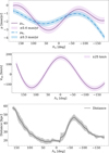 |
Fig. 1 Best-fit proper motions (upper panel) and line-of-sight velocity (middle panel) functions described by the expressions given in Eqs. (1) and (2), respectively. Their coefficients are shown in Table 1. The shaded regions in the proper motion plot show the confidence intervals (see Figs. 2b and 2c of Ibata et al. (2020) to contrast the polynomials with the stars’ distribution) such that the stream stars selected by I+2020 have a contamination of 11%. The shaded region in the radial velocity plot corresponds to half the interval that selects stars with a global contamination of 18% according to I+2020. Bottom panel: moving average Galactocentric distance as a function of the longitude, Λ⊙, for the set of stars given in Vasiliev et al. (2021), with the shaded gray region representing the corresponding moving average error along the stream. |
Fit coefficients.
3 Gravitational potentials and progenitor orbit
3.1 Milky Way potential
The strategy to fix the Galactic potential on which the spray simulations are performed is inspired by the work developed in Gibbons et al. (2014). From that work, it is possible to obtain the accumulated (total) mass of the host at different radii, such that it maximizes the likelihood of having the required (i.e., observed) apocentric Galactocentric distances of the Sgr stream’s arms and their angular difference. They used measurements from Belokurov et al. (2014), which are approximately aL = 47. 8 ± 0.5 kpc for the leading arm apocenter, aT = 102.5 ± 2.5 kpc for the trailing one, and ψ = 99.3° ± 3.5° for the (heliocentric) opening angle between both given apocenters. These values are in agreement with the ones given by Hernitschek et al. (2017), who measures aL = 47.8 ± 0.5 kpc, aT = 98.95 ± 1.3 kpc, and ψ = 104.4° ± 1.3°. The corresponding accumulated Galaxy masses are reported in Fig. 13 and Table 3 of Gibbons et al. (2014), from which we chose a three-tuple of DM-mass values (i.e., once the baryonic component was extracted, see below) for each DM potential. Each tuple is conformed of the enclosed DM mass at three different characteristic scales where the stream moves: inner (r = 12 kpc), mid (r = 40 kpc), and outer (r = 80 kpc), shown in Table 3. These selected masses to be fulfilled by the DM models belong to 2σ mass dispersion interval reported in Fig. 13 of Gibbons et al. (2014).
Given the large number of ejected stars (∼ 105), it takes about 40 hours of CPU time within our Python code to predict one Sgr stream, precluding us from running a Monte Carlo algorithm on the model parameters. This is why we present only four different simulations, with a conveniently fixed DM model for each: three different RAR models with different degrees of accumulated mass from inner to outer halo Galaxy scales, and a Burkert model for comparison (see below for details). On the other hand, the baryonic component of the Galaxy is modeled as the combination of three main components: a bulge and two disks (thick and thin), based on Pouliasis et al. (2017). The bulge is described through a Plummer sphere, while the thin and thick disks are modeled by the Miyamoto-Nagai formula (Miyamoto & Nagai 1975). Such baryonic models have gravitational potentials of the form:
![Mathematical equation: \[{{\Phi }_{MN}}(R,z)=-\frac{GM}{\sqrt{{{R}^{2}}+{{(a+\sqrt{{{z}^{2}}+{{b}^{2}}})}^{2}}}},\]](/articles/aa/full_html/2025/07/aa50867-24/aa50867-24-eq7.png) (3)
(3)
![Mathematical equation: \[{{\Phi }_{P}}(r)=-\frac{GM}{\sqrt{{{r}^{2}}+{{b}^{2}}}},\]](/articles/aa/full_html/2025/07/aa50867-24/aa50867-24-eq8.png) (4)
(4)
where MN stands for Miyamoto–Nagai and P for Plummer. The values of the free parameter for each baryonic component are given in Table 2.
Regarding the DM component, we followed the RAR model (Argüelles et al. 2018), sometimes referred to in the literature as the relativistic fermionic King model. This is a semi-analytical model based on a self-gravitating system of neutral fermions, derived from first physical principles. It is based on the knowledge of a most likely coarse-grained phase-space distribution function (DF) of the fermions at (violent) relaxation. It was obtained by applying a maximum entropy production principle on an adequate kinetic theory coupled with gravity (Chavanis 2004). Such a DF is of the Fermi-Dirac type (see Eq. (3) in Argüelles et al. 2018) and it includes two phenomena. One is the Pauli exclusion principle (i.e., fermion degeneracy), causing a dense fermion core at the center of the halo that acts as an alternative to the SMBH scenario. On the other hand, it is the effect of escape of particles that leads to finite-sized halos. Once there is this most likely fermionic DF, the equation of state (E.o.S, ρ(r), P(r)) is built as corresponding momentum integrals of this DF, in order to obtain the DM profile by solving a coupled system of equilibrium equations for appropriate boundary conditions taken from galactic observables. The equilibrium equations of the RAR model are obtained by solving the Einstein (general relativistic) equations in spherical symmetry, sourced by a perfect fluid ansatz with the above (ρ(r), P(r)) E.o.S, and read (in dimensionless form):
![Mathematical equation: \[\begin{matrix} \frac{d\hat{M}}{d\hat{r}}=4\pi {{{\hat{r}}}^{2}}\hat{\rho } \\ \frac{dv}{d\hat{r}}=\frac{2(\hat{M}+4\pi \hat{P}{{{\hat{r}}}^{3}})}{{{{\hat{r}}}^{2}}(1-2\hat{M}/\hat{r})}, \\ \frac{d\theta }{d\hat{r}}=-\frac{1-{{\beta }_{0}}(\theta -{{\theta }_{0}})}{{{\beta }_{0}}}\frac{\hat{M}+4\pi \hat{P}{{{\hat{r}}}^{3}}}{{{{\hat{r}}}^{2}}(1-2\hat{M}/\hat{r})}, \\ \beta (\hat{r})={{\beta }_{0}}{{e}^{\frac{{{v}_{0}}-v(\hat{r})}{2}}}, \\ W(\hat{r})={{W}_{0}}+\theta (\hat{r})-{{\theta }_{0}}. \\\end{matrix}\]](/articles/aa/full_html/2025/07/aa50867-24/aa50867-24-eq9.png) (5)
(5)
The dimensionless quantities are: ![Mathematical equation: \[\hat{r}=r/\chi ,\hat{M}=GM/({{c}^{2}}\chi ),\hat{\rho }=G{{\chi }^{2}}\rho /{{c}^{2}},\hat{P}=G{{\chi }^{2}}P/{{c}^{4}}\]](/articles/aa/full_html/2025/07/aa50867-24/aa50867-24-eq10.png) , with χ = 2π3/2(ħ/(mc))(mp/m) and
, with χ = 2π3/2(ħ/(mc))(mp/m) and ![Mathematical equation: \[{{m}_{p}}=\sqrt{\hbar c/G}\]](/articles/aa/full_html/2025/07/aa50867-24/aa50867-24-eq11.png) the Planck mass. The system of Eq. (5) constitute an initial value problem, which, for a fixed DM particle mass, m, has to be solved for a given set of free parameters (β0, θ0, W0) defined at the center of the configuration.
the Planck mass. The system of Eq. (5) constitute an initial value problem, which, for a fixed DM particle mass, m, has to be solved for a given set of free parameters (β0, θ0, W0) defined at the center of the configuration.
The first two are the only relevant Einstein equations (mass and Tolman-Oppenheimer–Volkoff equations), the third and fourth are obtained from the Tolman and Klein relations for a gas in thermodynamic equilibrium in General Relativity (GR), and the fifth corresponds to particle energy conservation along a geodesic (see Argüelles et al. 2018 and refs. therein for details). The density and pressure (ρ(r), P(r)) of the system are varying (nonanalytic) functions of the radius (see Eqs. (2), (3) in Argüelles et al. 2021). The nonlinear system of (ordinary) coupled differential equations written above implies an initial condition problem for the variables M(0) = M0 = 0, y(0) = y0, W(0) = W0, θ(0) = θ0, and β(0) = β0, where the subscript 0 indicates that they are evaluated at the center of the configuration. The function M(r) is the enclosed mass at radius r, and ν(r) is the metric potential matching with the Schwarzchild potential at the boundary, ensuring this condition through the value of ν0 (see Argüelles et al. 2021 for details). The functions W(r), θ(r), and β(r) are named as the cutoff, degeneracy, and temperature variables, respectively (for an equivalent setup of the fermionic equations and for the numerical scheme actually used to solve them in this paper, see, respectively, Sect. 2.2 and Appendix A in Mestre et al. 2024).
Such a model depends on four free parameters: the degeneracy parameter, θ0, the cutoff parameter, W0, the temperature parameter, β0, and the DM particle mass, m. This set of free parameters provides a solution for the mass distribution, whose characteristics strongly depend upon the galaxy type (see e.g., Krut et al. 2023 for an allowed window of RAR free parameters in agreement with disk galaxies from the SPARC dataset, and Argüelles et al. 2018, 2019 for the MW and other galaxy types, respectively). Because of this, we generated different RAR halos whose gravitational potential (together with the baryonic counterpart) were used to run the spray algorithm, allowing us to study how the different profiles change the features of the stream. We used four different profiles, three of them of a fermionic nature, named as RAR 1, RAR 2, RAR 3, and a Burkert one (Burkert 1995). Their specifications are explained as follows:
The DM model RAR 1 is defined according to the set of free parameters found in Becerra-Vergara et al. (2020, 2021) for the MW. For such a set of parameters, with m = 56 keV, it was proved that the DM halo is of a core–halo nature, where the dense and compact DM core can fit the orbits of the S-cluster stars without assuming a BH (Becerra-Vergara et al. 2021). At the same time, the outer halo develops a tail of polytropic trend such that the overall profile can reproduce the so-called grand rotation curve of the Galaxy (ranging from parsec scales up to scales of tens of kiloparsecs according to the data provided in Sofue 2013). The motivation for choosing this specific fermionic model (originally aimed at fitting the rotation curve of the Galaxy together with the S-cluster stars’ orbits) was just to check how it stands with respect to an independent tracer of the Galactic potential, such as the Sgr stream. The accumulated DM mass of this model fulfills the specific values at four different radii (central, inner, mid, and outer) as reported in Table 3.
The DM models RAR 2 and RAR 3 were asked to fulfill (within a 2σ dispersion) with selected accumulated total mass values, as was inferred in Gibbons et al. (2014) from the observed apocentric distances of the leading and trailing arms of the stream and their opening angle (see Fig. 13 and Table 3 of that work), and reported in Table 3. These mass values are close to the mass constraints from Vasiliev et al. (2021): M(r = 50 kpc) = (3.85 ± 0.1) × 1011 M⊙ and M(r = 100 kpc) = (5.7 ± 0.3) × 1011 M⊙. RAR 2 and RAR 3 differ from the RAR 1 case on outer halo scales as follows: the DM mass of the RAR 2 profile at 12 kpc is roughly twice as massive as the RAR 1 at the same radius, while RAR 3 is almost 70% more massive than RAR 1 at the same scale (the mass of the fermion core is asked to be the same in all cases). Since the leading arm apocenter is most sensitive to the accumulated mass profile in the [10–60] kpc radial window, then considerable differences in the behavior of M(r) in such a window are expected to lead to noticeable changes in the predictions of the shape of the corresponding part of the stream (see e.g., Figs. 7–12). Another difference between RAR 2 and RAR 3 on halo scales is the accumulated mass at the outermost radii 80 kpc, which in the latter case is roughly twice as large as in the former. Given the allowed physics of the fermionic model, this implies that the morphology of the outer halo tail of RAR 3 develops a more extended power-law-like trend similar to Burkert (and different from polytropic). A thing such as that is achieved for a lower particle mass than in the first two RAR cases. Finally, since the compacity of the DM core sensitively depends on the fermion mass, only the solutions of m = 56 keV can provide enough compact cores to work as a good alternative to the BH in SgrA*, as is demonstrated in Becerra-Vergara et al. (2020, 2021); Argüelles et al. (2022).
-
The Burkert profile is a two-free parameter DM density pro-file with a power law behavior, ∝ r−3, for the halo tail, given by the equation:
![Mathematical equation: \[{{\rho }_{Bur}}(r)=\frac{{{\rho }_{0}}}{(\frac{r}{{{r}_{0}}}+1)[{{(\frac{r}{{{r}_{0}}})}^{2}}+1]},\]](/articles/aa/full_html/2025/07/aa50867-24/aa50867-24-eq12.png) (6)
(6)and shown in Fig. 2. It was chosen in order to make a comparison between a typical model used in the literature obtained within ΛWDM cosmologies, and the (similar) power-law-like trend of the DM halo in the RAR 3 case. The density parameter, ρ0, is the density at the origin of the distribution, i.e., ρ0 = ρ(0). On the other hand, r0 corresponds to a halo-scale radius where the density satisfies ρ(r0) = ρ0/4. The values of the best-fit parameters from this model are given in Table 4 in agreement with the specific accumulated masses of Table 3 (see Sect. 5 for a discussion about the similitude in the predictions of the stream between Burkert and the RAR 3 model).
To find the best values of the free parameters in the RAR and Burkert models, we used a differential evolution algorithm5 to fit the predicted enclosed mass to the values in Table 3, adopting an allowed “error” in fitting such boundary mass values to the RAR models of ∼ 10%. The corresponding best-fit parameters (β0, θ0, W0) for the fermionic models, and (ρ0, r0) for the Burkert one are given in Table 4, while the corresponding mass and density profiles are given in Fig. 2.
Coefficients of the Galactic baryonic components.
Mass values of the host.
Free parameter values.
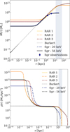 |
Fig. 2 Top panel: RAR enclosed mass profiles corresponding to the best-fit parameters given in Table 4, which satisfy the enclosed mass values in Table 3 and Section 3.2, respectively for the MW and the Sgr dwarf. Additionally, we display the fit Burkert profile for comparison. Bottom panel: Profiles corresponding to the density of the same DM halos considered in the upper panel. In both panels, the shaded region indicates where the progenitor will move in its orbit around the Galaxy. |
3.2 Potential of the progenitor
It has been proven that the gravitational attraction of the satellite is needed to correctly reproduce the stellar stream ejected by Sgr. For example, Gibbons et al. (2014) used a spray method to generate a stellar stream and studied the same tidal stream with and without the self-gravity of the satellite. The resulting stream embedded in the gravitational potential of the host and the progenitor agreed with the results of the N–body simulations they made.
To model the progenitor of the stream, we considered that it is formed by two components, a baryonic component and a DM one. This choice is suggested in Vasiliev & Belokurov (2020), in which it is argued that a single baryonic component progenitor cannot match all the observational constraints. We adopted a Plummer sphere of mass 108 M⊙ and scale length bSgr = 0.3 kpc to model the baryons of this galaxy. Afterward, we performed a best fit on a RAR DM halo constrained by two data points for the accumulated DM mass of the Sgr galaxy: M(1.55 kpc) = (1.2 ± 0.6) × 108 M⊙ and M(4 kpc) = (4.5 ± 0.7) × 108 M⊙. The former constraint was taken from Walker et al. (2009), while the latter one is in agreement with the value estimated in Vasiliev & Belokurov (2020): M(5 kpc) = (4 ± 1) × 108 M⊙. Due to the facts that (i) our spray algorithm uses a constant progenitor potential, and (ii) we are interested in studying specially the last 3 Gyr of evolution, we decided that it was more realistic to model the progenitor according to current observations instead of using estimated values at infall.
Of course, the particle mass for the halo of the progenitor is always chosen, for consistency, to be the same as the one involved in the DM of the given host (for each of the three RAR cases). In the first two cases (m = 56 keV), the halo model for the progenitor is named as Sgr56, and Sgr20 is used for the RAR 3 (m = 20 keV) and Burkert models. The enclosed mass values and density profiles of the Sgr models are shown in Fig. 2.
3.3 Orbit of the progenitor in the Galactic potential
Since we would use a spray algorithm to model the stellar stream generated by Sgr in its orbit all around the host, we needed first to compute the path of the progenitor backward in time. This was done before evolving the corresponding trajectory forward in time, while ejecting stars from the progenitor. This way, the orbit of the ejected stars could be integrated under the combined gravitational potential of the host and the satellite.
To integrate the progenitor orbit, a set of initial conditions was needed to give to the integrator. These were the position and velocity of the progenitor, which were taken from Gibbons et al. (2014), except for the heliocentric line-of-sight velocity, which was taken from Vasiliev & Belokurov (2020). These collected observables are detailed in Table 5.
Since the Galactocentric distance of the progenitor is not very well constrained, we let it vary through the different models to get orbits with approximately the same apocenter, chosen to agree with the values obtained in Law et al. (2005). In either case, they imply small differences in the pericentric distance, as the pericentric distance, t for the backwards integration time, and vc(R⊙) for the circular velocity at R⊙. Distances are in kiloparsecs, the time in gigayears, and the circular velocity in kilometers per second. can be seen in Table 6. Besides, when performing the backward integration in time, we did not select the same interval length for all the models. This was done in order to obtain roughly similar initial positions for the spray algorithm. All these considerations, together with the predicted circular velocity at the Galactocentric solar distance, R⊙, for each MW model, are summarized in Table 6.
Before integrating the orbit, the initial conditions were transformed to the Galactocentric reference frame, using the parameters detailed in Sect. 2. Summing up, we integrated four progenitor orbits, all of them sharing the same baryonic potential but each one with a different DM halo.
The integrated orbits of Sgr projected in the x − z plane for the four different potentials are shown in Fig. 4. Despite little differences in the orbits, they share the same general features, which are the number of pericentric passages, the area covered by each petal, the pericentric and apocentric distances, and (approximately) the time interval they took to complete the same number of petals. The small differences between the orbits arise because the gravitational field, under the assumption of spherical symmetry satisfied by the RAR and Burkert models, depends on the accumulated mass. This is better seen in Fig. 3, where the shaded region marks the limits of the orbits. Inside this region, the four DM components have different accumulated masses, generating different gravitational fields along the radial window of interest. Notice that the RAR 2 model, which is the most massive in the 20–30 kpc range, produces the orbit with the fastest precession rate.
Galactic coordinates of the Sagittarius dSph satellite.
Orbital parameters of the Sagittarius dSph.
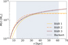 |
Fig. 3 Enclosed masses for the four dark halo models studied, but in the Galactocentric scales where the orbit of the satellite resides. The shaded region denotes the limits of this orbit. |
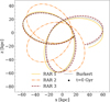 |
Fig. 4 Orbits of the Sgr dSph integrated backward in time projected in the x − z plane of the Galactocentric system. The orbits corresponding to the four models under consideration are shown. The black dot denotes the region where the backward integrations start. |
4 Stream generation
A spray algorithm is a procedure whereby the initial conditions of stars belonging to the progenitor are generated to be integrated with the combined gravitational potential of the progenitor and the host galaxy. Since each initial condition generated represents a star, the number of initial conditions will define the number of stars that compose the stream. We applied the spray algorithm as it was defined in Gibbons et al. (2014), but using a different prescription for the tidal radius (rt).
The spray procedure provides the initial position and velocity of each star ejected from the progenitor. According to Gibbons et al. (2014), the initial position of the stars at time t corresponds approximately with the Lagrange points, L1 and L2. We located both points, following the standard procedure, at a distance rt from the center of the satellite, so the L1 point was located at a Galactocentric radius r − rt while the L2 point was located at r + rt.
Various works argue for an appropriate description of the tidal radius. We followed the recipe from Gajda & Lokas (2016), in which an expression is derived of the tidal radius for a satellite orbiting a host galaxy, allowing for a rotating progenitor. This recipe has the form:
![Mathematical equation: \[{{r}_{t}}=r{{(\frac{[m({{r}_{t}})/M(r)]\lambda (r)}{2{{\Omega }_{s}}/\Omega -1+[2-p(r)]\lambda (r)})}^{1/3}}.\]](/articles/aa/full_html/2025/07/aa50867-24/aa50867-24-eq13.png) (7)
(7)
The denominator of the above expression must be greater than zero; otherwise, the tidal radius does not exist. In such a case, the acceleration of the star points towards the satellite and the tidal radius is interpreted as being infinite, which is precluded because Gajda & Lokas (2016) assumed that rt ≪ r. The quantities λ(r) and p(r) are ![Mathematical equation: \[\lambda (r)=\Omega _{circ~}^{2}(r)/{{\Omega }^{2}}\]](/articles/aa/full_html/2025/07/aa50867-24/aa50867-24-eq14.png) and p(r) = d lnM(r)/d lnr, respectively. Ω is the instantaneous angular velocity of the satellite, Ωcirc(r) is the angular velocity of a circular orbit at radius r and Ωs is the angular velocity of a given star respect to the satellite. Assuming that the stars to be ejected are located at the instantaneous Lagrange points, we set Ωs = Ω. Besides, we approximated m(rt) with the total mass of the satellite, msat.
and p(r) = d lnM(r)/d lnr, respectively. Ω is the instantaneous angular velocity of the satellite, Ωcirc(r) is the angular velocity of a circular orbit at radius r and Ωs is the angular velocity of a given star respect to the satellite. Assuming that the stars to be ejected are located at the instantaneous Lagrange points, we set Ωs = Ω. Besides, we approximated m(rt) with the total mass of the satellite, msat.
Before proceeding, it is necessary to remark on an important assumption regarding the tidal radius. The model of Gajda & Lokas (2016) was derived under spherical symmetry, and we are modeling the MW disk as composed of two baryonic axisymmetric components. Hence, to avoid such inconsistency, we computed the logarithmic derivative of M(r) in the formula for rt considering only the DM (spherical) component. This assumption was, in part, motivated by the estimated value of the radius of the baryonic disk of the MW. It has been argued in different papers (Sale et al. 2010; Minniti et al. 2011) that the stellar density of stars in the Galaxy has a drastic drop-off at a Galactocentric distance of R ∼ 13 kpc, which is the same order as the pericentric radii in our simulations. The temporal evolution of the tidal radius of each gravitational model of Table 4 can be seen in Fig. 5.
The value of the tidal radius varies along the given progenitor’s orbit due to the variation in time of the different quantities on which the tidal radius depends, i.e., the instantaneous orbital angular velocity of the satellite and the Galactocentric distance. The condition 1 + [2 − p(r)]λ(r) > 0 was checked in each time step at which the tidal radius was computed.
Regarding the velocities with which the stars will be ejected, they will be taken randomly from a multivariate Gaussian distribution whose mean is the Galactocentric velocity of the satellite at that time, and the dispersion is the velocity dispersion tensor of the progenitor. To model the latter, we assumed that it is diagonal and isotropic, i.e., all its components are the same, σ.
The Sgr dwarf spheroidal is far from dynamical equilibrium due to the strong tidal forces acting on it, and it has for a long time been orbiting the MW and being disrupted. So, when we mention the velocity dispersion of the Sgr galaxy, we are referring to the progenitor of the stream, which is the bound central region of the whole stellar structure. The value of σ that we adopted is σ = 11.4 km/s, taken from Ibata et al. (1997).
We generated four stellar streams, one for each MW’s gravitational potential. In order to do so, we ejected ∼ 105 stars, one half from L1 and the other half from L2. The ejection process was carried out at the same time that the progenitor evolved in its orbit to the future, finishing its trajectory at the black dot point of Fig. 4. Each ejection was represented by an initial position and velocity, following the recipe previously introduced. Once the initial condition was created, it was used as input for an integrator whose function was to compute the trajectory of such a star under host and satellite potentials. The integration occurs from the ejection time until the present (t = 0 Gyr). Since we were not considering the force exerted by the individual stars, the integration of the orbit of each of them was completely independent of the others, enabling the parallelization of the process.
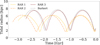 |
Fig. 5 Tidal radius evolution for each model of gravitational potential considered in this work. The time intervals at which each one was computed differ according to the parameters given in Table 6. |
5 Comparing the model with data and discussion
The final position of all the stars in the Galactocentric x − z plane of the generated stream is shown in Fig. 6, color-coded by the ejection time, starting ∼ 3 Gyr in the past. The black dots and the solid green line represent the Vasiliev et al. (2021) stars and the past orbit of the progenitor. It can be seen that the different models produce different stream configurations of their tails (e.g. length, width, orientation), though they all agree on the fact of developing a clear bifurcation in their corresponding trailing tail. Interestingly, the RAR 2 stream configuration resembles the output of the N-body simulation shown in Fig. 2 of Gibbons et al. (2014) with regard to the orientation of the trailing tail and the significant presence of the second wrap of their corresponding leading tails. In order to avoid the emergence of the complementary and more feeble sinusoidal structure of the dynamically older part of the stream, for which there is scarce data, in the rest of the plots we display only mock stars stripped at times later than t = −1.5 Gyr. Transforming the four mock streams to the reference system of I+2020, in the configuration space we display the Galactocentric distance of the stars, D, as a function of Λ⊙, as it is shown in Fig. 7.
With respect to the distribution of ejected stars in the D–Λ⊙ space, it is clear from Fig. 7 that none of the four DM models can correctly reproduce the shape of the leading tail. All of them generate an arm that lies closer to the Galactic center than the observations. This behavior can also be seen in Fig. 6, in which the leading tail reaches its maximum extent and then turns back instead of following the observed trend. Despite this discrepancy, it is worth noting that the RAR 3 and Burkert models (both power-law-like) achieve a slightly better agreement with the observed distance trend, making the mock stream fall less sharply with increasing negative longitude. Regarding the trailing arm, the four models agree very well with the observations, and among them, there are no remarkable differences in the predictions, as is the case for the leading tail.
Looking more deeply at Fig. 7, it can be seen that the leading arm centered at Λ⊙ ∼ − 50° has a “peak” shape. This phenomenon defines a maximum distance of the leading arm stars from the Galactic center. The same behavior occurs with the trailing arm. These two maximum distances define the leading and trailing (Galactocentric) apocentric distances, respectively. Thus, we fit a Gaussian function to each distribution of stars composing the arms. To properly delineate the shape of the leading tail, we considered stars ejected at t ≳ − 2 Gyr. In the case of the trailing arm, we took those stars with an ejection time t ≲ − 2 Gyr. The corresponding Gaussian functions are plotted in Fig. 8, in which there is one curve for each DM model considered. The apocentric distances associated with each model and each arm are given in Table 7, along with the heliocentric angular aperture between said apocenters.
Comparing the results of Table 7 with the ones reported in Belokurov et al. (2014) and Hernitschek et al. (2017), it can be seen that our models underestimate the Galactocentric trailing apocentric distance (e.g., by ∼ 25% for RAR 3), while overestimate the observed value of the heliocentric angular aperture (e.g., by ∼ 20% for RAR 3). On the other hand, there is a much better agreement between our predicted leading apocentric distances and the ones reported in Belokurov et al. (2014) and Hernitschek et al. (2017).
As a complementary analysis, in Fig. 9 the four circular velocity profiles corresponding to each DM model are displayed. In spite of the fact that the four models behave differently from one another regarding the circular velocity (or similarly, the acceleration field at z = 0), each one falls relatively well within the 95% confidence region of the best-fit model of Gibbons et al. (2014).
We also computed the star distributions in the velocity space, showing the predicted stream in the ![Mathematical equation: \[{{\Lambda }_{\odot }}-{{\mu }_{{{B}_{\odot }}}},{{\Lambda }_{\odot }}-{{\mu }_{{{\Lambda }_{\odot }}}}\]](/articles/aa/full_html/2025/07/aa50867-24/aa50867-24-eq15.png) , and Λ⊙ − Vlos planes, trying to reproduce the curves of Fig. 1. The result is shown, respectively, in Figs. 10, 11 and 12. In each one of the figures, Figs. 6, 7, and 10–12, we display one plot for each of the four models studied. In addition, we computed the time of ejection of each of the stars, encoded in the color bar.
, and Λ⊙ − Vlos planes, trying to reproduce the curves of Fig. 1. The result is shown, respectively, in Figs. 10, 11 and 12. In each one of the figures, Figs. 6, 7, and 10–12, we display one plot for each of the four models studied. In addition, we computed the time of ejection of each of the stars, encoded in the color bar.
In Figs. 10 and 11, the shaded region corresponds to a contamination of 11% in the stream stars selected by I+2020. As can be seen, the trailing tail of the stellar stream resides in this region in each of the eight figures, but not the part of the stream with negative values of Λ⊙. This section of the stream corresponds to the youngest piece of the leading tail. This suggests that the gravitational potentials tested here are unable to reproduce the entire observables independently of the type of halo tail considered (i.e., power-law-like or polytropic), or of the degree of DM mass concentration in the Galactocentric range of 10–60 kpc. The same type of discrepant behavior is seen in Fig. 12. This kind of disagreement is not new, and it is typical of DM models with spherical symmetry applied to model the Sgr stream (see, e.g., discussions in Helmi 2004; Law & Majewski 2010). However, the first-principle physics core–halo (RAR) profiles have never been tested before with the Sgr stream. We have for the first time exploited the flexibility of such a fermionic model, showing the extent of success of the theory when confronted with full 6D phase-space data. It is only after this first step that one can start to properly explore further extensions allowed by the fermionic theory, such as the inclusion of the LMC or some degree of asphericity in the DM halo, left for future work. As an additional advantage, the dense fermion core developed in the cases with m = 56 keV works as an alternative to the BH scenario by reproducing the orbits of the S-cluster stars (Becerra-Vergara et al. 2020, 2021).
Comparing in more detail the degree of success between the models studied here, it is worth noting that the power law profiles (i.e., RAR 3 and Burkert) achieve a slightly better agreement with the leading arm polynomial observables than the polytropic profiles (RAR 1 and RAR 2). Specifically, their distribution of stars in the leading tail for both proper motions and the line-of-sight velocity are less steep than in the polytropic cases. Although the extent of the leading arm is more sensitive to the accumulated mass in the first 10–60 kpc, the above comparison between the RAR models suggests that higher values of halo mass within the 30–60 kpc are preferable. On the other hand, the more extended power law density profiles, with correspondingly larger total halo masses with respect to the polytropic cases, seem not to improve in a considerable manner the trailing tail fitting.
Coming back to the discussion about spherically symmetric halos, evidence has suggested in the past that a spherical DM halo cannot reproduce the entire set of observables. For example, in Helmi (2004), it was shown for the first time that modeling the dark halo of our Galaxy as a prolate one is the preferred option over other symmetries, for the region probed by the dynamically old debris (2–4 Gyr) from the leading arm. On the other hand, Johnston et al. (2005) used M giant stars of tidal debris associated with Sgr to fit the simulated precession of the satellite’s orbit. They found that the best DM halo potential is one with slightly flattened potential contours. Thus, the difference with Helmi (2004) is that they determined that oblate dark halos are preferred over prolate ones. This is because the prolate halos can fit the Sgr leading arm radial velocities, but at the same time they cannot reproduce a stream fitting the precession of the progenitor, whereas oblate halos achieve the opposite.
This is why later on, in Law & Majewski (2010), an N– body model of the Sgr disruption was developed under the (ad-hoc) assumption of triaxiality for the dark halo, in order to better reproduce the stream. This non-axisymmetric potential fits the majority of angular position, distance, and radial velocity observables of the tidal debris of the progenitor. They determined that this triaxial component is a near-oblate ellipsoid whose minor axis lies in the Galactic disk plane. This is an unlikely dynamical configuration, so they suggest that the orientation may have evolved with time or that the need for triaxiality may have been obviated by introducing another non-axisymmetric component. Such a component could be a time-dependent perturbation exerted by a massive satellite of the MW, such as the Magellanic Clouds.
Moreover, a more sophisticated study carried out by Vasiliev et al. (2021) find a misalignment between the track of the stream and the direction of the reflex-corrected proper motions in the leading tail. They tested models without the presence of the LMC and find that these models cannot solve the mentioned misalignment and, additionally, they overestimate the distance to the leading arm apocenter. In that same paper, they propose as a solution to this problem that there is a time-dependent perturbation acting on the whole stellar system. This perturbation may arise because of the presence of the LMC. They show that the stream can be modeled up to a certain extent by taking into account the gravitational pull exerted by the LMC on our Galaxy (reflex motion) and on the Sgr system (dwarf and stream). They are able to provide a flexible mathematical function (depending on 11 free parameters) for the DM halo, which is able to make predictions in agreement with all the available observations. The complexity in this kind of phenomenological modeling includes radially varying axis ratios and orientations. The inner part of it is oblate, with the minor axis lying perpendicular to the Galactic disk, while the outer one is another oblate ellipsoid whose minor axis lies almost in the Galactic plane. The degree of success of this model makes Vasiliev et al. (2021) a state-of-the-art description of the Sgr stellar stream.
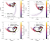 |
Fig. 6 Streams of stars projected in the x − z plane at present, color-coded by the ejection time. The black dots represent the x–z coordinates of the Vasiliev et al. (2021) stars. The solid green lines indicate the orbit of the satellite in its corresponding gravitational potential. |
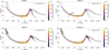 |
Fig. 7 Streams of stars in the D–Λ⊙ space at present color-coded by the ejection time. The solid black curve represents the distance trend of the Vasiliev et al. (2021) stars, while the shaded region is the distance error, both quantities being moving means as a function of the longitude, Λ⊙. The distances are referred to the Galactocentric reference frame. |
Stream morphological parameters.
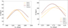 |
Fig. 8 Analytic functions tracing the Galactocentric distance of both main tails of the Sgr stellar stream, the leading one (left plot) and the trailing one (right plot). Every curve is a Gaussian function, whose maximum represents the value of its corresponding apocentric distance. The location of the maximum is the longitude, Λ⊙, of the corresponding apocenter, used to compute the heliocentric angular aperture. There is one curve for each DM model considered in the work. |
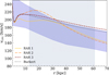 |
Fig. 9 Circular velocity profiles for each DM model studied in this work. The shaded gray region represents the zone where the progenitor moves along its way around the MW. The shaded blue region denotes the reproduced 95% confidence region of the best-fit circular velocity curve of Gibbons et al. (2014). Note that the four circular velocity curves agree relatively well with the best-fit prediction, despite slight differences at upper marginal values. At the same time, for r ≳ 40 kpc the polytropic profiles (RAR 1 and RAR 2) fall sharper than the power-law-like profiles (RAR 3 and Burkert), as was expected based on Fig. 3. |
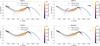 |
Fig. 10 Mock stream star |
![Mathematical equation: \[{{\mu }_{{{B}_{\odot }}}}\]](/articles/aa/full_html/2025/07/aa50867-24/aa50867-24-eq16.png)
![Mathematical equation: \[{{\mu }_{{{\Lambda }_{\odot }}}}\]](/articles/aa/full_html/2025/07/aa50867-24/aa50867-24-eq17.png)
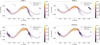 |
Fig. 12 Line-of-sight velocity component of the stars of the four predicted streams at present, color-coded with their ejection time. The solid black line represents the fit line-of-sight velocity as a function of Λ⊙ computed by I+2020, based on the Law & Majewski (2010) model. The shaded pink region represents the limits to account for Galactic field star contaminants, though here it was used a more stringent value than in I+2020 to reduce the contamination fraction. |
6 Conclusions
In this work, we have tested for the first time in the literature a fermionic DM halo model based on first-principle physics, such as (quantum) statistical mechanics and thermodynamics (i.e., the RAR distribution), against Sgr stellar stream observations. This is to try to reproduce the 6D phase-space properties of the Sgr tidal stream with the aim of assessing the fermionic model. This self-gravitating system of neutral fermions has properties that make it a very good candidate to model galactic halos, as has recently been shown in Krut et al. (2023) for a sample of 120 different galaxies. Moreover, as is demonstrated in Argüelles et al. (2021), this fermionic core–halo profile with particle mass range in the sub-megaelectronvolt range can arise at late stages of non-linear structure formation in cosmology, making it a promising case to be compared with other phenomenological profiles.
Using baryonic potentials in combination with RAR DM halos, we have modeled the gravitational potential for both the MW and the Sgr dwarf. After introducing a spray algorithm and a tidal radius model, we applied them to create adequate initial conditions to integrate the orbit of individual stars, in order to generate four stellar streams based on four different dark halo models. The data we used to compare with the theory is that of Ibata et al. (2020) and Vasiliev et al. (2021): the Cartesian Galactocentric coordinates of stars, where a distance trend was derived, and three polynomials functions taking into account the proper motions and line-of-sight velocity behavior of stars in the Sgr debris.
As the main conclusion, we find that across the different families of fermionic halo models (i.e., power-law-like and polytropic ones), they can only reproduce the trailing arm of the Sgr stream. Within the observationally allowed span of enclosed masses where the stream moves, none of the RAR halo profiles can answer for the observed trend of the leading tail. This is a conclusion that coincides with the results from other types of spherically symmetric halos studied in the literature. Nevertheless, our spherically symmetric fermionic models do agree with the observed apocentric distance of the leading arm (see Fig. 8). If one considers the previous success of this fermionic halos when contrasted with different halo tracers of our Galaxy, such as the GD-1 cold stream (Mestre et al. 2024) or the ones associated with rotation curves analysis (Argüelles et al. 2018; Becerra-Vergara et al. 2020; Argüelles & Collazo 2023), the more complex Sgr stream tracer studied here puts a firm limit on the applicability of this first-principle physics theory on outer halo scales. Indeed, the knowledge and tests done in this work can now be used to further extend the model by including the effects of the LMC and possibly add some degree of triaxiality, which may well be associated with an out-of-equilibrium DM component acquired within the merger history of the Galaxy. Further improvements to our theory may include more sophisticated models for stream generation, such as the restricted N-body simulations developed in Vasiliev et al. (2021) or Ibata et al. (2024).
As was already mentioned above for the MW, the motivation to maintain this kind of core–halo fermionic models in future, more sophisticated analyses, is based on the success it has already achieved in explaining: (i) the rotation curve data of different galaxies (Argüelles et al. 2019; Krut et al. 2023); (ii) the universal galaxy scaling relations among different galaxy types (Argüelles et al. 2019; Krut et al. 2023); (iii) the formation and stability of fermionic profiles in a cosmological framework, as well as the existence of a critical point of DM core-collapse toward a supermassive BH (Argüelles et al. 2021, 2023b, 2024); (iv) the explanation of the MW rotation curve and the phase-space track of the GD-1 stellar stream together with the astrometric data of the central S-stars (without assuming a BH), (Becerra-Vergara et al. 2020, 2021; Argüelles et al. 2022; Mestre et al. 2024); and (v) the prediction of the relativistic images and spectra around the central core when illuminated by an accretion disk (Pelle et al. 2024).
In addition, we have consistently used the same fermion mass for both MW and Sgr dwarf halos. Moreover, the total enclosed mass of the dark halo of Sgr in the polytropic RAR profiles agrees with the estimates of the actual mass of the remnant discussed in Vasiliev & Belokurov (2020) and in Vasiliev et al. (2021).
As a final remark, we stress that models depending on physically inspired free parameters are complementary to state-of-the-art MW halo models (which depend on several free parameters with consequent high degeneracy) and may help in the task of better reproducing the Sgr observations. This is why we believe that DM halo models such as the one shown here are worth further investigation in the field of stellar streams.
Acknowledgements
The authors would like to thank Rodrigo Ibata for providing us with valuable observational data of the Sgr stream. We also thank Daniel Carpintero for fruitful discussions. We thank the IALP support staff for their dedicated work. The authors deeply appreciate the reviewer’s exhaustive assessment of the manuscript and their valuable suggestions, which greatly improved its clarity and rigor. SC acknowledges financial support from CONICET. MFM acknowledges support from CONICET (PIP2169) and from the Universidad Nacional de La Plata (PID G178). CRA acknowledges support from CONICET, the ANPCyT (grant PICT-2020-02990), and ICRANet. SC and CRA acknowledge support from Universidad Nacional de La Plata (PID G175).
References
- Antoja, T., Ramos, P., Mateu, C., et al. 2020, A&A, 635, L3 [NASA ADS] [CrossRef] [EDP Sciences] [Google Scholar]
- Argüelles, C. R., Becerra-Vergara, E. A., Rueda, J. A., & Ruffini, R. 2023a, Universe, 9, 197 [Google Scholar]
- Argüelles, C. R., Boshkayev, K., Krut, A., et al. 2023b, MNRAS, 523, 2209 [Google Scholar]
- Argüelles, C. R., & Collazo, S. 2023, Universe, 9, 372 [Google Scholar]
- Argüelles, C., Krut, A., Rueda, J., & Ruffini, R. 2018, Phys. Dark Universe, 21, 82 [CrossRef] [Google Scholar]
- Argüelles, C., Krut, A., Rueda, J., & Ruffini, R. 2019, Phys. Dark Universe, 24, 100278 [CrossRef] [Google Scholar]
- Argüelles, C. R., Díaz, M. I., Krut, A., & Yunis, R. 2021, MNRAS, 502, 4227 [CrossRef] [Google Scholar]
- Argüelles, C. R., Mestre, M. F., Becerra-Vergara, E. A., et al. 2022, MNRAS, 511, L35 [CrossRef] [Google Scholar]
- Argüelles, C. R., Rueda, J. A., & Ruffini, R. 2024, ApJ, 961, L10 [Google Scholar]
- Becerra-Vergara, E. A., Argüelles, C. R., Krut, A., Rueda, J. A., & Ruffini, R. 2020, A&A, 641, A34 [NASA ADS] [CrossRef] [EDP Sciences] [Google Scholar]
- Becerra-Vergara, E. A., Argüelles, C. R., Krut, A., Rueda, J. A., & Ruffini, R. 2021, MNRAS, 505, L64 [NASA ADS] [CrossRef] [Google Scholar]
- Belokurov, V., Evans, N. W., Irwin, M. J., et al. 2007, ApJ, 658, 337 [Google Scholar]
- Belokurov, V., Koposov, S. E., Evans, N. W., et al. 2014, MNRAS, 437, 116 [NASA ADS] [CrossRef] [Google Scholar]
- Bonaca, A., & Hogg, D. W. 2018, ApJ, 867, 101 [NASA ADS] [CrossRef] [Google Scholar]
- Bonaca, A., & Price-Whelan, A. M. 2024, arXiv e-prints, [arXiv:2405.19410] [Google Scholar]
- Bowden, A., Belokurov, V., & Evans, N. W. 2015, MNRAS, 449, 1391 [NASA ADS] [CrossRef] [Google Scholar]
- Burkert, A. 1995, ApJ, 447, L25 [NASA ADS] [Google Scholar]
- Chavanis, P.-H. 2004, Physica A, 332, 89 [CrossRef] [MathSciNet] [Google Scholar]
- Chavanis, P.-H., Lemou, M., & Méhats, F. 2015, Phys. Rev. D, 92, 123527 [NASA ADS] [CrossRef] [Google Scholar]
- Debattista, V. P., Roškar, R., Valluri, M., et al. 2013, MNRAS, 434, 2971 [NASA ADS] [CrossRef] [Google Scholar]
- Deg, N., & Widrow, L. 2013, MNRAS, 428, 912 [Google Scholar]
- Dierickx, M. I. P., & Loeb, A. 2017, ApJ, 836, 92 [NASA ADS] [CrossRef] [Google Scholar]
- Dinescu, D. I., Majewski, S. R., Girard, T. M., et al. 2002, ApJ, 575, L67 [Google Scholar]
- Fardal, M. A., Huang, S., & Weinberg, M. D. 2015, MNRAS, 452, 301 [NASA ADS] [CrossRef] [Google Scholar]
- Fardal, M. A., van der Marel, R. P., Law, D. R., et al. 2019, MNRAS, 483, 4724 [NASA ADS] [CrossRef] [Google Scholar]
- Gajda, G., & Lokas, E. L. 2016, ApJ, 819, 20 [NASA ADS] [CrossRef] [Google Scholar]
- Gibbons, S. L. J., Belokurov, V., & Evans, N. W. 2014, MNRAS, 445, 3788 [NASA ADS] [CrossRef] [Google Scholar]
- GRAVITY Collaboration (Abuter, R., et al.) 2018, A&A, 615, L15 [NASA ADS] [CrossRef] [EDP Sciences] [Google Scholar]
- Grillmair, C. J., & Dionatos, O. 2006, ApJ, 643, L17 [Google Scholar]
- Hawkins, K., Price-Whelan, A. M., Sheffield, A. A., et al. 2023, ApJ, 948, 123 [NASA ADS] [CrossRef] [Google Scholar]
- Helmi, A. 2004, ApJ, 610, L97 [NASA ADS] [CrossRef] [Google Scholar]
- Hernitschek, N., Sesar, B., Rix, H.-W., et al. 2017, ApJ, 850, 96 [NASA ADS] [CrossRef] [Google Scholar]
- Huxor, A. P., & Grebel, E. K. 2015, MNRAS, 453, 2653 [Google Scholar]
- Ibata, R. A., Gilmore, G., & Irwin, M. J. 1994, Nature, 370, 194 [Google Scholar]
- Ibata, R. A., Wyse, R. F. G., Gilmore, G., Irwin, M. J., & Suntzeff, N. B. 1997, AJ, 113, 634 [Google Scholar]
- Ibata, R., Lewis, G. F., Irwin, M., Totten, E., & Quinn, T. 2001, ApJ, 551, 294 [Google Scholar]
- Ibata, R., Bellazzini, M., Thomas, G., et al. 2020, ApJ, 891, L19 [NASA ADS] [CrossRef] [Google Scholar]
- Ibata, R., Malhan, K., Tenachi, W., et al. 2024, ApJ, 967, 89 [NASA ADS] [CrossRef] [Google Scholar]
- Johnston, K. V., Law, D. R., & Majewski, S. R. 2005, ApJ, 619, 800 [Google Scholar]
- Koposov, S. E., Belokurov, V., Evans, N. W., et al. 2012, ApJ, 750, 80 [NASA ADS] [CrossRef] [Google Scholar]
- Koposov, S. E., Belokurov, V., & Evans, N. W. 2013, ApJ, 766, 79 [Google Scholar]
- Koposov, S. E., Belokurov, V., Li, T. S., et al. 2019, MNRAS, 485, 4726 [Google Scholar]
- Krut, A., Argüelles, C. R., Chavanis, P. H., Rueda, J. A., & Ruffini, R. 2023, ApJ, 945, 1 [NASA ADS] [CrossRef] [Google Scholar]
- Küpper, A. H. W., Lane, R. R., & Heggie, D. C. 2012, MNRAS, 420, 2700 [Google Scholar]
- Law, D. R., & Majewski, S. R. 2010, ApJ, 714, 229 [Google Scholar]
- Law, D. R., Johnston, K. V., & Majewski, S. R. 2005, ApJ, 619, 807 [Google Scholar]
- Law, D. R., Majewski, S. R., & Johnston, K. V. 2009, ApJ, 703, L67 [NASA ADS] [CrossRef] [Google Scholar]
- Li, T. S., Koposov, S. E., Zucker, D. B., et al. 2019, MNRAS, 490, 3508 [NASA ADS] [CrossRef] [Google Scholar]
- Luque, E., Pieres, A., Santiago, B., et al. 2017, MNRAS, 468, 97 [NASA ADS] [CrossRef] [Google Scholar]
- Majewski, S. R., Siegel, M. H., Kunkel, W. E., et al. 1999, AJ, 118, 1709 [Google Scholar]
- Majewski, S. R., Skrutskie, M. F., Weinberg, M. D., & Ostheimer, J. C. 2003, ApJ, 599, 1082 [NASA ADS] [CrossRef] [Google Scholar]
- Majewski, S. R., Kunkel, W. E., Law, D. R., et al. 2004, AJ, 128, 245 [Google Scholar]
- Malhan, K., & Ibata, R. A. 2018, MNRAS, 477, 4063 [Google Scholar]
- Mateo, M., Olszewski, E. W., & Morrison, H. L. 1998, ApJ, 508, L55 [NASA ADS] [CrossRef] [Google Scholar]
- Mateu, C. 2023, MNRAS, 520, 5225 [Google Scholar]
- Mestre, M. F., Argüelles, C. R., Carpintero, D. D., Crespi, V., & Krut, A. 2024, A&A, 689, A194 [NASA ADS] [CrossRef] [EDP Sciences] [Google Scholar]
- Minniti, D., Saito, R. K., Alonso-García, J., Lucas, P. W., & Hempel, M. 2011, ApJ, 733, L43 [Google Scholar]
- Miyamoto, M., & Nagai, R. 1975, PASJ, 27, 533 [NASA ADS] [Google Scholar]
- Newberg, H. J., Yanny, B., Rockosi, C., et al. 2002, ApJ, 569, 245 [Google Scholar]
- Newberg, H. J., Yanny, B., Grebel, E. K., et al. 2003, ApJ, 596, L191 [Google Scholar]
- Newberg, H. J., Yanny, B., Cole, N., et al. 2007, ApJ, 668, 221 [Google Scholar]
- Pelle, J., Argüelles, C. R., Vieyro, F. L., et al. 2024, MNRAS, 534, 1217 [Google Scholar]
- Pouliasis, E., Di Matteo, P., & Haywood, M. 2017, A&A, 598, A66 [NASA ADS] [CrossRef] [EDP Sciences] [Google Scholar]
- Ramos, P., Mateu, C., Antoja, T., et al. 2020, A&A, 638, A104 [EDP Sciences] [Google Scholar]
- Reid, M. J., Menten, K. M., Brunthaler, A., et al. 2014, ApJ, 783, 130 [Google Scholar]
- Robles, V. H., Lora, V., Matos, T., & Sánchez-Salcedo, F. J. 2015, ApJ, 810, 99 [Google Scholar]
- Ruffini, R., Argüelles, C. R., & Rueda, J. A. 2015, MNRAS, 451, 622 [CrossRef] [Google Scholar]
- Sale, S. E., Drew, J. E., Knigge, C., et al. 2010, MNRAS, 402, 713 [Google Scholar]
- Schönrich, R., Binney, J., & Dehnen, W. 2010, MNRAS, 403, 1829 [NASA ADS] [CrossRef] [Google Scholar]
- Slater, C. T., Bell, E. F., Schlafly, E. F., et al. 2013, ApJ, 762, 6 [NASA ADS] [CrossRef] [Google Scholar]
- Sofue, Y. 2013, PASJ, 65, 118 [NASA ADS] [Google Scholar]
- Springel, V. 2005, MNRAS, 364, 1105 [Google Scholar]
- Totten, E. J., & Irwin, M. J. 1998, MNRAS, 294, 1 [Google Scholar]
- Varghese, A., Ibata, R., & Lewis, G. F. 2011, MNRAS, 417, 198 [NASA ADS] [CrossRef] [Google Scholar]
- Vasiliev, E., & Belokurov, V. 2020, MNRAS, 497, 4162 [Google Scholar]
- Vasiliev, E., Belokurov, V., & Erkal, D. 2021, MNRAS, 501, 2279 [NASA ADS] [CrossRef] [Google Scholar]
- Virtanen, P., Gommers, R., Oliphant, T. E., et al. 2020, Nat. Methods, 17, 261 [Google Scholar]
- Walker, M. G., Mateo, M., Olszewski, E. W., et al. 2009, ApJ, 704, 1274 [Google Scholar]
- Wang, H.-F., Hammer, F., Yang, Y.-B., & Wang, J.-L. 2022, ApJ, 940, L3 [CrossRef] [Google Scholar]
- Yanny, B., Newberg, H. J., Johnson, J. A., et al. 2009, ApJ, 700, 1282 [NASA ADS] [CrossRef] [Google Scholar]
In Debattista et al. (2013), the authors proved how difficult it is to reconcile the Law & Majewski (2010) model (in which the minor axis of the baryonic disk is aligned with the intermediate axis of the DM halo) with CDM halo predictions due to an instability issue.
By the term “cored”, we refer to the fact that the profiles present a “plateau” at inner halo scales. This is not to be confused with the degenerate and compact core at milliparsec scales of the core–halo distribution, such as the model studied here. Our model has both a central compact core and a plateau at the halo.
Our model dependent vc(R⊙) does not influence the simulations, nor the transformation of the observed data.
![Mathematical equation: \[{{\mu }_{{{\Lambda }_{\odot }}}}\]](/articles/aa/full_html/2025/07/aa50867-24/aa50867-24-eq18.png) includes the cos(B⊙) factor throughout this work.
includes the cos(B⊙) factor throughout this work.
We used an implementation from the SciPy libray (Virtanen et al. 2020), called optimize.differential_evolution algorithm, with metaparameters given by strategy=“best2bin”.
All Tables
All Figures
|
Fig. 1 Best-fit proper motions (upper panel) and line-of-sight velocity (middle panel) functions described by the expressions given in Eqs. (1) and (2), respectively. Their coefficients are shown in Table 1. The shaded regions in the proper motion plot show the confidence intervals (see Figs. 2b and 2c of Ibata et al. (2020) to contrast the polynomials with the stars’ distribution) such that the stream stars selected by I+2020 have a contamination of 11%. The shaded region in the radial velocity plot corresponds to half the interval that selects stars with a global contamination of 18% according to I+2020. Bottom panel: moving average Galactocentric distance as a function of the longitude, Λ⊙, for the set of stars given in Vasiliev et al. (2021), with the shaded gray region representing the corresponding moving average error along the stream. |
| In the text | |
|
Fig. 2 Top panel: RAR enclosed mass profiles corresponding to the best-fit parameters given in Table 4, which satisfy the enclosed mass values in Table 3 and Section 3.2, respectively for the MW and the Sgr dwarf. Additionally, we display the fit Burkert profile for comparison. Bottom panel: Profiles corresponding to the density of the same DM halos considered in the upper panel. In both panels, the shaded region indicates where the progenitor will move in its orbit around the Galaxy. |
| In the text | |
|
Fig. 3 Enclosed masses for the four dark halo models studied, but in the Galactocentric scales where the orbit of the satellite resides. The shaded region denotes the limits of this orbit. |
| In the text | |
|
Fig. 4 Orbits of the Sgr dSph integrated backward in time projected in the x − z plane of the Galactocentric system. The orbits corresponding to the four models under consideration are shown. The black dot denotes the region where the backward integrations start. |
| In the text | |
|
Fig. 5 Tidal radius evolution for each model of gravitational potential considered in this work. The time intervals at which each one was computed differ according to the parameters given in Table 6. |
| In the text | |
|
Fig. 6 Streams of stars projected in the x − z plane at present, color-coded by the ejection time. The black dots represent the x–z coordinates of the Vasiliev et al. (2021) stars. The solid green lines indicate the orbit of the satellite in its corresponding gravitational potential. |
| In the text | |
|
Fig. 7 Streams of stars in the D–Λ⊙ space at present color-coded by the ejection time. The solid black curve represents the distance trend of the Vasiliev et al. (2021) stars, while the shaded region is the distance error, both quantities being moving means as a function of the longitude, Λ⊙. The distances are referred to the Galactocentric reference frame. |
| In the text | |
|
Fig. 8 Analytic functions tracing the Galactocentric distance of both main tails of the Sgr stellar stream, the leading one (left plot) and the trailing one (right plot). Every curve is a Gaussian function, whose maximum represents the value of its corresponding apocentric distance. The location of the maximum is the longitude, Λ⊙, of the corresponding apocenter, used to compute the heliocentric angular aperture. There is one curve for each DM model considered in the work. |
| In the text | |
|
Fig. 9 Circular velocity profiles for each DM model studied in this work. The shaded gray region represents the zone where the progenitor moves along its way around the MW. The shaded blue region denotes the reproduced 95% confidence region of the best-fit circular velocity curve of Gibbons et al. (2014). Note that the four circular velocity curves agree relatively well with the best-fit prediction, despite slight differences at upper marginal values. At the same time, for r ≳ 40 kpc the polytropic profiles (RAR 1 and RAR 2) fall sharper than the power-law-like profiles (RAR 3 and Burkert), as was expected based on Fig. 3. |
| In the text | |
|
Fig. 10 Mock stream star |
| In the text | |
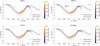 |
Fig. 11 Same as in Fig. 10, but for the |
| In the text | |
|
Fig. 12 Line-of-sight velocity component of the stars of the four predicted streams at present, color-coded with their ejection time. The solid black line represents the fit line-of-sight velocity as a function of Λ⊙ computed by I+2020, based on the Law & Majewski (2010) model. The shaded pink region represents the limits to account for Galactic field star contaminants, though here it was used a more stringent value than in I+2020 to reduce the contamination fraction. |
| In the text | |
Current usage metrics show cumulative count of Article Views (full-text article views including HTML views, PDF and ePub downloads, according to the available data) and Abstracts Views on Vision4Press platform.
Data correspond to usage on the plateform after 2015. The current usage metrics is available 48-96 hours after online publication and is updated daily on week days.
Initial download of the metrics may take a while.