| Issue |
A&A
Volume 698, June 2025
|
|
|---|---|---|
| Article Number | A265 | |
| Number of page(s) | 11 | |
| Section | Extragalactic astronomy | |
| DOI | https://doi.org/10.1051/0004-6361/202553747 | |
| Published online | 20 June 2025 | |
Optical quasi periodic oscillations with dual periodicities of 1103 days and 243 days in the blue quasar SDSS J100438.8+151056
School of Physical Science and Technology, GuangXi University, No.100, Daxue East Road, Nanning 530004, PR China
⋆ Corresponding author: This email address is being protected from spambots. You need JavaScript enabled to view it.
Received:
14
January
2025
Accepted:
9
May
2025
Abstract
This manuscript investigates the possible existence of a binary supermassive black hole (BSMBH) system in the blue quasar SDSS J100438.8+151056 (= SDSS J1004+1510) at z = 0.219 based on the detection of robust optical quasi periodic oscillations (QPOs). We determine QPOs using multiple analysis methods applied to the Catalina Sky Survey (CSS) V-band, Zwicky Transient Facility (ZTF) g-band and r-band light curves, and additionally, combined with the characteristics of broad emission lines, we explore potential mechanisms for the QPOs, including jet and disk precession models. Two distinct periodicities, 1103±260 days and 243±29 days, are identified in the ZTF g-band and r-band light curves with a confidence level exceeding 5σ, through four different techniques. Meanwhile, the 1103±260 days periodicity is also clearly detected in the CSS V-band light curve. The optical periodicities suggest a BSMBH system candidate in SDSS J1004+1510, with an estimated total virial black hole (BH) mass of (1.13±0.14)×108 M⊙ and a space separation of 0.0053±0.0016 pc for the periodicity of 1103±260 days. The second periodicity, of 243±29 days, could be attributed to harmonic oscillations, considering (1103±260)/(243±29)∼4.54±0.47 with large scatters. However, if the periodicity of 243±29 days was from an independent QPO, a triple BH system candidate on a subparsec scale could probably be expected, with space separations of 0.00036±0.00004 pc within a close BSMBH system and of 0.0053±0.0016 pc between the BSMBH system and the third BH, after considering the similar BH mass of the third BH as the total mass of the central BSMBH. These findings strongly demonstrate that combined light curves from different sky survey projects can lead to more reliable QPO candidates being detected, and also indicate that higher-quality light curves could probably be helpful in finding potential QPOs with multiple periodicities, leading to rare detections of candidates for subparsec triple BH systems.
Key words: galaxies: active / galaxies: nuclei / quasars: emission lines / quasars: supermassive black holes / quasars: individual: SDSS J1004+1510
© The Authors 2025
 Open Access article, published by EDP Sciences, under the terms of the Creative Commons Attribution License (https://creativecommons.org/licenses/by/4.0), which permits unrestricted use, distribution, and reproduction in any medium, provided the original work is properly cited.
This article is published in open access under the Subscribe to Open model. This email address is being protected from spambots. You need JavaScript enabled to view it. to support open access publication.
1. Introduction
Galaxy merging is an important part of the formation and evolution of galaxies in the Universe (Carlberg 1992; Kauffmann et al. 1993; Lacey & Cole 1994; Barnes & Hernquist 1996; Silk & Rees 1998; Menou et al. 2001; Lin et al. 2004; Bundy et al. 2009; Merritt 2006; Satyapal et al. 2014; Rodriguez et al. 2016, 2017; Bottrell et al. 2019; Martin et al. 2021; Jackson et al. 2021; Yoon et al. 2022; Lokas 2023, and Kim et al. 2024). Almost every galaxy has a BH at its center (Kormendy & Richstone 1995; Ferrarese & Ford 2005; Kormendy & Ho 2013, and Heckman & Best 2014). This means that the process of galaxy merger is often accompanied by the formation of dual active galactic nuclei (dual AGN) on a kiloparsec scale and binary supermassive black hole (BSMBH) systems on a subparsec scale (Begelman et al. 1980; Morgan et al. 2010; Fragione et al. 2019; Yang et al. 2019, and Mannerkoski et al. 2022). When galaxies merge, the BHs at their centers, due to dynamical friction (Merritt & Milosavljevic 2005 and Chen et al. 2020), gradually move closer to each other and orbit around a common center of mass, forming a dual AGN on a kiloparsec scale. As time goes on, gravitational wave radiation becomes the main mechanism driving the BHs even closer together, and eventually the distance between them shrinks to a subparsec scale, forming a tightly packed BSMBH system. These two BHs may further merge to form a larger supermassive BH (SMBH), releasing strong gravitational waves at the same time (Ehlers et al. 1976; Flanagan & Cutler 1994; Centrella et al. 2010; Hughes 2009). The study of dual AGN and BSMBHs is one of the hotspots of current research and is crucial for understanding the coevolution of SMBHs and galaxies.
Dual AGN systems on kiloparsec scales have been widely observed and studied through directly resolved images. However, subparsec-scale BSMBH systems have rarely been detected through directly resolved images, and the extremely close proximity between the BHs in BSMBH systems makes observation and identification very difficult using photometric images. Even with the help of high-resolution techniques such as the Very Long Baseline Interferometry Array (VLBA), only a few successes have been reported. For example, Rodriguez et al. (2006) discovered a BSMBH system within the radio galaxy 0402+379. This discovery was made possible through the use of VLBA, which provided high-resolution imaging of two compact, variable, and active nuclei within the galaxy, these nuclei having a projected separation of about 7.3 pc. In addition, Kharb et al. (2017) also report another subparsec-scale BSMBH candidate with a separation of approximately 0.35 pc in NGC 7674 through VLBA.
Given the limitations of direct imaging observations, scientists have also attempted to use a variety of indirect observational methods to explore the subparsec-scale BSMBH systems in recent years. Among these, spectroscopic characterization is an important tool. For example, by observing the double-peaked features of broad emission lines in the spectra of quasars, (Lauer & Boroson 2009; Shields et al. 2009; Tsalmantza et al. 2011; Eracleous et al. 2012; Shen et al. 2013; Liu et al. 2014; Runnoe et al. 2015, and Wang et al. 2017) have analyzed the velocity variations of these broad emission lines. Their findings provide evidence supporting the probable existence of subparsec-scale BSMBH systems.
Besides the applications of unique spectroscopic features of broad emission lines, the detection of quasi periodic oscillations(QPOs) in long-term light curves is also an important and convenient indicator for identifying subparsec-scale BSMBH candidates. Many research teams have reported QPOs in AGN with periodicities ranging from hundreds to thousands of days. These QPOs can be caused by a variety of physical mechanisms, including jet precession (Marscher & Gear 1985; Camenzind & Krockenberger 1992; Abraham 2000; Caproni et al. 2013; Huang et al. 2021), BH tidal disruption events (Shu et al. 2020), accretion disk instabilities (Vietri & Stella 1998; Tsang & Lai 2009; Pihajoki et al. 2013), general relativistic effects (Stella & Vietri 1998; Stella et al. 1999; Ingram et al. 2016), and orbital motions of BSMBH systems (Kormendy et al. 2009; Gaskell 2010; Barth et al. 2015; Songsheng et al. 2020). Although the origin of QPOs in light curves is complex, most reported QPOs are considered to be from the orbital motions of BSMBH systems. For example, Graham et al. (2015a) detect and report a 5.2 yr periodicity in the quasar PG 1302-102, attributed to the orbital motion of a BSMBH system. In a follow-up study, Graham et al. (2015b) conducted a systematic search for QPOs in light curves of 243 500 sources from the Catalina Real-Time Transient Survey (CRTS). This search has led to the identification of 111 potential BSMBH candidates. The light curve characteristics of these candidates, as validated by theoretical models, were found to be consistent with the periodic variations expected from BSMBH systems. Similarly, Liu et al. (2015), Graham et al. (2015a, b), Charisi et al. (2016), Li et al. (2016), Zheng et al. (2016), Kovacevic et al. (2020), Serafinelli et al. (2020), Liao et al. (2021), and O’Neill et al. (2022) have also reported subparsec-scale BSMBH candidates based on QPOs detected in the light curves. Additionally, in our recent studies on QPOs (Zhang 2022a, b, 2023a, 2025a), we also identify such BSMBH candidates in broad-line AGN.
QPOs play a key role in detecting BSMBH systems in galaxies; however, relying on QPO signals for detections can present some accuracy challenges. First, the time durations of the light curves are monitored as a key factor because the detection of QPO signals needs to rely on long-term time-series data to ensure that the observed periodic variations are not chance events. In addition, the stochastic AGN variability may produce signals similar to QPOs, as Sesana et al. (2018) and Vaughan et al. (2016) discuss. To improve the accuracy of detections of QPOs and to reduce false-positive results, it is crucial to select light curves with long-term and continuous observational data. Among the public sky surveys, the Catalina Sky Survey (CSS) (Mahabal et al. 2011; Drake et al. 2009) has sufficient temporal baseline and sky coverage to provide favorable conditions for searching for long-lived optical QPOs. In addition, the high-frequency observing capability of the Zwicky Transient Telescope (ZTF) (Bellm et al. 2019; Dekany et al. 2020) provides a finer light curve for capturing optical QPOs with shorter periods. Combining the long-term light curves of the CSS with the ZTF allows for more efficient identifications and analysis of optical QPOs. In the recent work of Zhang (2022b, 2025a), the author combined the observations of the CSS with ZTF at different time periods to obtain light-variation data up to 16 years, which provide important clues for detecting more reliable optical QPOs.
In this manuscript, through the combined light curves from CSS and ZTF, we report the discovery of a potential BSMBH system in the blue quasar SDSS J100438.8+151056 (= SDSS J1004+1510) (redshift of 0.219), which is not reported in the sample of Graham et al. (2015b), probably due to the short time duration of the CSS V-band light curve of SDSS J1004+1510 relative to its periodicity. After analyzing the CSS V-band light curve, an optical QPO signal with a periodicity of around 1000 days can be detected. Moreover, QPOs with a periodicity around 220 days can be detected in the higher-quality ZTF g-band and r-band light curves, besides the periodicity around 1000 days. Section 2 of this paper presents the optical QPOs through four analytical methods applied to the long-term optical light curves of SDSS J1004+1510. Section 3 focuses on the spectroscopic results. Section 4 discusses the probable central BSMBH system and the possibility of dual-periodic signals probably related to a triple BH system candidate. Finally, our conclusions are given in Section 5. In this paper, the cosmological parameters have been adopted as H0 = 70 km s−1 Mpc−1, ΩΛ = 0.7, and Ωm = 0.3.
2. Optical QPOs in SDSS J1004+1510
2.1. Long-term optical light curves of SDSS J1004+1510
The long-term light curves in the observer frame of SDSS J1004+1510 can be collected from the CSS1 and ZTF2. The CSS V-band light curve was collected with MJD-53000 from 469 (March 2005) to 3592 (November 2013). And the ZTF g-band and r-band light curves were collected with MJD-53000 from 5202 (March 2018) to 6996 (March 2023). As the ZTF i-band light curve only includes 53 data points in a short time duration, it was not considered for this paper. The collected light curves are shown in the top left panel of Fig. 1.
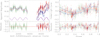 |
Fig. 1. Top left panel: Light curves from the CSS (solid circles plus error bars in green) and from the ZTF in the g band (minus 0.35 mag) (open circles plus error bars in blue) and r band (minus 0.35 mag) (open circles plus error bars in red), alongside the best-fitting results (solid lines in red) from a sinusoidal function plus a fourth-degree polynomial component. The solid purple lines represent the component described by the sinusoidal function (plus 17.5 mag), while the dashed purple lines indicate the component modeled by the polynomial function. The solid blue lines indicate the corresponding 5σ confidence bands to the best-fitting results through the F-test technique. Top right panel: Phase-folded light curves based on the determined periodicity 985 days (with the polynomial trends subtracted; green for CSS data, blue for ZTF g band, and red for ZTF r band) along with the best sinusoidal fit (solid line in red). The same as the top left panel for the solid blue lines. Bottom panels: Corresponding residuals (light curves minus the best-fitting results), with the solid red line denoting the residuals = 0. |
2.2. The analyses of QPOs in SDSS J1004+1510
Similarly to our recent approach in Zhang (2022b, 2023a, 2025a), we applied the following four methods to determine the probable QPOs in SDSS J1004+1510: the direct fitting method, the phase-folded method, the generalized Lomb-Scargle (GLS) method (Lomb 1976; Scargle 1982; Bretthorst 2001; Zechmeister & Kurster 2009; VanderPlas 2018; Springford et al. 2020), and the weighted wavelet Z-transform (WWZ) method (Foster 1996; An et al. 2016; Gupta et al. 2018; Kushwaha et al. 2020; Liao et al. 2021).
The light curves were first described by the direct fitting method, with a sinusoidal function plus a fourth-degree polynomial component simultaneously applied to each light curve from the CSS and the ZTF. The sinusoidal function was specifically chosen to capture the periodic variations in the light curve without delving into the physical origins of the QPOs, while the fourth-degree polynomial was used to represent long-term nonperiodic trends. The model functions are described as
 (1)
(1)
While the model functions are applied, the parameter of TQPO is the same for each light curve. To ensure the best fit, the Levenberg-Marquardt least-squares method was used to optimize the parameters of these composite models. The model parameters determined are presented in Table 1, with the periodicity determined to be approximately 985±8 days. The best-fitting results and the corresponding 99.99994% (5σ) confidence bands (determined by the F-test technique) are shown in the top left panel of Figure 1, with χ2/d.o.f. = 8847.144/827∼10.69. The residuals (the differences between the observed data and the model predictions) are shown in the bottom left panel of Figure 1.
Parameter values for the LMC model function.
Besides the model functions of Equation (1), if only the fourth-degree polynomial components are used to describe each light curve, this will lead to  . To assess the significance of the sinusoidal components, the F-test technique was employed to compare models with and without the sinusoidal component. The F-test statistic was calculated as
 (2)
(2)
Based on the given confidence level (5σ), the numerator degree of freedom (d.o.f.1−d.o.f.), and the denominator degree of freedom (d.o.f.), the corresponding F-distribution value was calculated as
 (3)
(3)
Therefore, through the F-test statistical technique, the sinusoidal component is preferred with a confidence level much higher than 5σ, indicating that the periodic fluctuations in the data seem to be a genuine feature rather than a random occurrence.
Based on the periodicity obtained from the direct-fitting method, the phase-folded method was applied to the light curves after subtracting the polynomial components. Through a simple sinusoidal function
 (4)
(4)
the folded light curves can be well described and are shown in the top right panel of Figure 1, with χ2/d.o.f. = 8860.0165/843 = 10.51, through the Levenberg-Marquardt least-squares minimization technique. The bottom right panel of Figure 1 shows the residuals (differences between the fitting results and the phase-folded light curves).
To further investigate the optical QPOs in SDSS J1004+1510, in addition to the direct-fitting method and the phase-folded method shown in Figure 1, the improved GLS method (see the Python astroML package) was also applied. Compared with the traditional Lomb-Scargle method, GLS is particularly suitable for handling unevenly sampled datasets, allowing for more accurate identification and quantification of periodic signals in time series.
Figure 2 presents the GLS periodogram results for the CSS V-band and the ZTF g-band and r-band light curves. In the CSS V-band light curve, a significant peak is detected, corresponding to a periodicity of about 1250±112 days (solid line in green), with a significance level higher than 99.99994%, along with a secondary, less prominent peak around 272±1 days (confidence level lower than 5σ). In the results from the GLS method for the high-quality ZTF g-band and r-band light curves (represented by blue and red lines, respectively), there are main peaks around 1165±30 days and 1000±30 days, with significance levels higher than 99.99994%. Interestingly, compared with the CSS V-band light curve, there are more prominent periodicities around 221±2 days and 215±1 days, respectively, both exceeding the 99.99994% confidence level. Based on the GLS periodogram applied to randomly created light curves including about half of the data points in the origin light curves, Figure 3 shows the distributions of peak periodicity in the CSS V-band and ZTF g-band and r-band light curves determined by the bootstrap method applied with 500 loops, leading to the determined uncertainties of the periodicities by the half width at half maximum of the distributions.
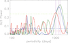 |
Fig. 2. Properties of the GLS periodogram. Solid lines in red, blue, and green show the corresponding results from the ZTF r-band, g-band, and CSS V-band light curves, respectively. The dashed horizontal lines in red, blue, and green indicate the corresponding 5σ confidence levels (FAP = 1–99.99994%) for the results from the ZTF r-band, g-band, and CSS V-band light curves, respectively. |
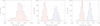 |
Fig. 3. Periodicity distributions through the bootstrap method. Left panel: Results for the CSS V-band light curve. Middle panel and right panel: Periodicities for the ZTF g-band (blue histogram) around 1165 days and 221 days, as well as for the ZTF r band (red histogram) around 990 days and 215 days. |
In addition, the WWZ method was also employed for an in-depth analysis of the CSS V band, ZTF g-band and r-band light curves. As shown in Figure 4, the power spectrum covered a frequency (in units of 1/day) range of 0.0005–0.01, with a frequency step of 0.00001. The result for the ZTF r-band light curve in the top panel reveals two distinct periodicities, one around 950±42 days and another around 270±3.5 days. In the middle panel for the ZTF g-band light curve, two significant periodicities are also observed: one around 1405±40 days and a shorter one around 225±3 days, while the bottom panel for the CSS V-band light curve shows a dominant periodicity around 1265±40 days, with a secondary periodicity around 265±3 days. The results obtained from the WWZ method are consistent with those derived from the GLS periodogram.
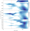 |
Fig. 4. Results of the WWZ analysis for the CSS V-band, the ZTF g-band and r-band light curves. For the ZTF r-band light curve (top panel), two periodicities are identified at approximately 950±42 days and 270±3.5 days. For the ZTF g-band light curve (middle panel), two periodicities are around 1405±40 days and 225±3 days. For the CSS V-band light curve (bottom panel), two periodicities are around 1265±40 days and 265±3 days. In each panel, the dashed vertical red lines mark the positions for the periodicities. |
Additionally, to determine the uncertainties of the periodicities detected by the WWZ method, the bootstrap technique was applied. More than half of the data points from the observed CSS V-band, ZTF g-band and r-band light curves were randomly collected to generate new light curves, with the process repeated 800 times. Subsequently, the WWZ method was used to determine the periodic distributions of these new light curves, and the results are shown in Figure 5. The uncertainties of the periodicities were determined by the half width at half maximum of the distributions.
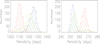 |
Fig. 5. Both panels: Distributions of WWZ-determined periodicities around 1000 days and 200 days, as determined by the bootstrap method. The green, blue, and red histograms show the results for the CSS V-band, the ZTF g-band and r-band light curves, respectively. |
Based on the secondary periodicity determined by the GLS method and the WWZ method, especially in the ZTF light curves, Figure 6 shows the results of refitting to the ZTF g-band and r-band light curves by using two sinusoidal functions. The model functions are expressed as
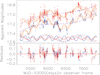 |
Fig. 6. Best-fitting results (top panel) and corresponding residuals (bottom panel) to the ZTF g/r-band light curves by two sinusoidal components. Top panel: Circles plus error bars in blue and in red show the ZTF g-band and r-band light curves, solid orange lines represent the best-fitting results, dashed orange lines indicate the 5σ (99.99994%) confidence bands, and dashed purple lines show the polynomial components. The dashed blue and solid blue lines show the sinusoidal components with periods of 1024±12 days and 222±1 days in the ZTF g-band light curve, and the dashed and solid lines in red represent the sinusoidal components with periods of 886±6 days and 257±1 days in the ZTF r-band light curve. |
 (5)
(5)
Then, through the Levenberg-Marquardt least-squares minimization technique, the best-fitting results can be determined and are shown in Figure 6 for the ZTF light curves, leading to χ2/d.o.f. = 7430.6168/728≈10.206. The model parameters determined, listed in Table 1, can be applied to support the secondary periodicities in the ZTF g-band and r-band light curves. Based on the model function used to fit the light curves in the left panel of Figure 1, when only the ZTF g-band and r-bands are fitted the resulting χ2/d.o.f. is calculated as 8767.5/734≈11.945. As demonstrated in Equations (2) and (3) above, the F-test technique was employed to compare the model containing one sinusoidal component with the model containing two sinusoidal components. The result of FP is about FP≈21.8, and the Fdis is about Fdis≈5.8 (based on the given confidence level of 5σ). These results indicate that the model with two sinusoidal components provides a better fit.
We applied four different techniques, including the direct-fitting method leading to the results shown in the left panel of Figures 1 and 6, the phase-folded method leading to the results shown in the right panel of Figure 1, the GLS periodogram leading to the results shown in Figure 2, and the WWZ method leading to the results shown in Figure 4. All of these methods lead to two significant periodicities in ZTF light curves. Meanwhile, for the CSS V-band light curve, a significant periodicity is detected by four methods, while the WWZ and GLS method also reveal an additional insignificant periodicity. Differences in detected short-period signals between the CSS and ZTF bands may be attributed to the higher temporal resolution and observational precision of ZTF light curves, which can reveal finer variability features, which the CSS V-band might have missed. In summary, there are two periodicities in SDSS J1004+1510, at 1103±260 days (1103 as the mean value of the longer periodicities of 985 days, 1024 days, 886 days, 1250 days, 1165 days, 1000 days, 1265 days, 1405 days, and 950 days from different techniques applied to different light curves, and the uncertainty 260 as half of the maximum difference among the longer periodicities) and 243±29 days (243 as the mean value of the shorter periodicities of 222 days, 257 days, 272 days, 221 days, 215 days, 265 days, 225 days, and 270 days, and the uncertainty 29 as half of the maximum difference among the shorter periodicities). The source of the above periodicities is shown in Table 2.
Periodicities detection methods and results.
2.3. Are optical QPOs related to the intrinsic AGN variability of SDSS J1004+1510?
Similarly to our recent approach in Zhang (2023a, 2025a,b), it was necessary to check the effects of red noise traced by intrinsic AGN activities on the detected optical QPOs in SDSS J1004+1510, accepted artificial light curves, LMCt (red noises, intrinsic AGN variability), being simulated by the continuous autoregressive (CAR) process (Kell et al. 2009; MacLeod et al. 2010; Kozłowski et al. 2010; Zu et al. 2013):
 (6)
(6)
where ϵ(t) is a white noise process with zero mean and variance equal to 1, bdt = 17.19 is the mean value of LMCt (with 17.19 as the mean value of the ZTF g-band light curve of SDSS J1004+1510), τ is the relaxation time of the process, and σ is the variability of the time series on a timescale shorter than τ. The uncertainties of the simulated light curves, LMCt, are given by  , with Lobs and Lerr as the observed ZTF g-band light curve and the corresponding uncertainties, as shown in the left panel of Figure 1.
Through the CAR process in Kell et al. (2009), two sets of 10 000 simulated light curves were generated. The first set had the same time information, t, as the actual observation time of CSS V-band and ZTF g-band light curves, with τ randomly selected from 50 days to 1000 days and the variance,  , from 0.005 to 0.02 as for the common values in quasars in MacLeod et al. (2010). The second set had the same time information as the observation time of the ZTF g-band light curve, with τ from 50 days to 1000 days and the variance,
  , from 0.005 to 0.02.
There are 15 light curves with detected QPOs that can be selected from the first set of simulated light curves, based on the following two criteria. First, the simulated light curves can be well described by Equation (1) with a corresponding χ2/d.o.f. smaller than 15 (χ2/d.o.f. = 10.69 in Fig. 1), and the periodicity determined is within the range of 1103±260 days. Second, the periodicity determined by the GLS method should be within 1103±260 days, with a significance level higher than 5σ. For the second set of simulated light curves, two light curves with expected detected QPOs can be selected if they meet the following two conditions. First, the simulated light curves must be well described by Equation (5) with a corresponding χ2/d.o.f. smaller than 15 (χ2/d.o.f. = 10.206 in Fig. 6), and the two periodicities determined should be within 1103±260 days and 243±29 days. Second, the periodicities determined by the GLS method should be within 1103±260 days and 243±29 days, with a significance level higher than 5σ. One example of these misdetected QPOs from each set of simulated light curves treated as red noise is shown in Figure 7.
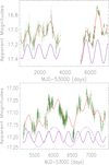 |
Fig. 7. Top panel: Example of probable misdetected QPOs in the first set of simulated light curves by the CAR process. Solid dark green circles plus error bars show the simulated light curve, solid lines in red show the best-fitting result by Equation (1), with χ2/d.o.f. = 6. The solid lines in purple show the sinusoidal component with a period of 910 days. Bottom panel: One of the probable misdetected QPOs in the second set of simulated light curves. Solid dark green circles plus error bars show the simulated light curve, and the solid line in red shows the best-fitting result by Equation (5), with χ2/d.o.f. = 1.13. The solid and dashed lines in purple show the sinusoidal components with periodicity of 263 days and 851 days, respectively. |
The results above indicate that the CAR process, which can be applied to trace red noise, can lead to misdetected QPOs in simulated light curves. However, after considering the effects of red noise, it can be confirmed that the probability is only 2/10 000 (corresponding to 3.7σ) for two periodicities detected over the ZTF observation time, and the probability is only 15/10 000 (corresponding to 3.17σ) for only the large periodicity over the combined CSS and ZTF observation time. Therefore, the detected QPOs in SDSS J1004+1510 are robust enough, even after considering the effects of red noise.
3. Spectroscopic results of SDSS J1004+1510
Considering that optical QPOs may be caused by the orbital motions of two BH accreting systems in an expected central BSMBH system in SDSS J1004+1510, these orbital motions could also have probable effects on the features of broad optical Balmer emission lines if the two related broad emission line regions (BLRs) were not totally mixed. Therefore, it is necessary to study the characteristics of the broad emission lines. Figure 8 displays the SDSS spectrum of SDSS J1004+1510, collected from SDSS DR16 (Ahumada et al. 2021) with PLATE-MJD-FIBERID = 2586-54169-0405. In this spectrum, prominent emission lines can be described by multiple Gaussian functions, as Zhang (2022a, 2023a) demonstrates utilizing a combination of broad and narrow Gaussian functions to precisely measure the emission lines.
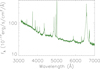 |
Fig. 8. SDSS spectrum of SDSS J1004+1510. |
To measure the emission lines around Hβ (rest wavelength from 4700 Å to 5100 Å ), the following model functions were utilized. For the broad and narrow Hβ emission lines, three broad Gaussian functions and two narrow Gaussian functions (one for the core component and the other for the extended component) were applied. For the [O III] λ4959 Å, 5007 Å doublet, three Gaussian functions were applied to each line to describe the core component, the extended component, and an additional intermediate extended component. Additionally, a power-law function was applied to describe the continuum emissions underneath the emission lines. Then, using the Levenberg-Marquardt least-squares minimization technique, the best-fitting results and the corresponding residuals of the emission lines around Hβ were determined and are shown in the top left panel of Figure 9, with χ2/d.o.f. = 1.1. Here, the corresponding residuals were determined by the spectrum minus the best-fitting results and then divided by the uncertainties of the spectrum. The model parameters determined are listed in Table 3.
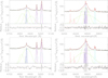 |
Fig. 9. Top panels: Fitting results and corresponding residuals for the emission lines around Hβ and Hα, respectively, considering three broad Gaussian components for broad Balmer lines. In the top left panel, the solid black line represents the observed SDSS spectrum, the solid red line indicates the best-fitting results, the green and blue lines show the broad and narrow Hβ components, and the solid cyan and purple lines represent the core and extended components of the [O III] doublet. In the top right panel, the solid black line represents the observed SDSS spectrum, the solid red line represents the best-fitting results, the solid green line illustrates the broad Gaussian components of Hα, the solid blue line represents the narrow Gaussian components in Hα, the solid purple line shows the core and extended components of the [N II] doublet, the solid cyan line represents the core and extended components in the [S II] doublet, and the solid pink line indicates the core and extended components in the [O I] doublet. In each top panel, the dashed green line represents the determined power-law continuum emissions. For each residual, the dashed horizontal red lines show residuals = ±1. In order to show clear features of the determined emission components, the plots are shown with y-axis in logarithmic. Similarly to the results presented in the top panels, bottom panels show the fitting results and the corresponding residuals for the emission lines around Hβ and Hα, respectively, considering two broad Gaussian components for broad Balmer lines. |
Line parameters.
For the emission lines around Hα (rest wavelength from 6200 Å to 6900 Å ), the following model functions were applied. Five Gaussian functions were applied to describe the broad and narrow Hα emission lines, with three Gaussian functions for the broad Hα and two for the narrow Hα. The [N II]λ6548 Å, 6583 Å doublet was described by four Gaussian functions for both the core and extended components. The [S II]λ6716 Å, 6731 Å doublet and the [O I]λ6300 Å, 6363 Å doublet were also fitted in a similar manner, with one Gaussian function for the core component and the other Gaussian function for the extended component in each line. A power-law function was used for the continuum emissions underneath the emission lines. Then, using the Levenberg-Marquardt least-squares minimization technique, the best-fitting results and the corresponding residuals were determined and are shown in the top right panel of Figure 9, with χ2/d.o.f. = 1.1. The model parameters determined are listed in Table 3.
To further analyze the significant physical information in the broad emission lines, the continuum and the narrow emission lines were subtracted from the spectra, leaving only the broad emission components of Hα and Hβ. The normalized broad Hα and Hβ are shown in velocity space in Figure 10, to show line profile comparisons between broad Hα and broad Hβ in SDSS J1004+1510. Meanwhile, based on the second moment definition of emission lines (Peterson et al. 2004), the measured linewidths of the broad Hα and broad Hβ are 2677.8±539 km/s and 1871.67±441.24 km/s (the uncertainty determined by the maximum error of σ for the broad Gaussian components in Table 3), respectively. It is evident that the linewidth of broad Hα is slightly wider than that of broad Hβ. However, as noted by Korista & Goad (2004), Bentz et al. (2010), and Netzer (2020), broad Hα, having the greatest intrinsic optical depth among the broad Balmer emission lines, would typically exhibit a narrower (or similar, but not broader) linewidth than broad Hβ. This suggests that intrinsic optical depth differences alone cannot explain the observed line profile variations. As Zhang (2023b) proposes, the distinct line profiles of broad Balmer emission lines are likely due to extrinsic obscuration differences between the two independent broad-line regions of the BSMBH system, providing support for the presence of central BSMBHs. Additionally, the peak velocities (relative to the rest-frame central wavelength) of Hα and Hβ are approximately −85.59±110.59 km/s and 241.18±543 km/s, respectively (the uncertainty determined by the maximum error of λ0 for the broad Gaussian components in Table 3). The significant shifted velocity difference also implies that if broad Hα and broad Hβ originated from probably different regions, an otherwise similar kinematic system should lead to similar peak velocities and similar linewidths (second moment). Therefore, the results above suggest the possible existence of two BLRs.
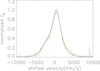 |
Fig. 10. Line-profile comparisons of broad Hα (in red) and broad Hβ (in green) in velocity space, after subtracting the continuum and all other narrow emission lines. |
Furthermore, the intensity ratio of broad Hα to broad Hβ can be calculated as 4.83, slightly greater than the theoretical value of 2.86, indicating that dust extinction might be present in the BLRs of SDSS J1004+1510, causing greater absorption of Hβ. However, while dust extinction could explain the intensity ratio greater than 2.86, it alone is insufficient to account for the velocity and profile differences between broad Hα and broad Hβ. Moreover, differences in optical depth may partially contribute to the differences in the profiles of broad Hα and broad Hβ, but they cannot solely explain the significant velocity shifts between broad Hα and broad Hβ.
In conclusion, the hypothesis of a BSMBH system is a more reasonable explanation: broad Hα and broad Hβ originate from two distinct BLRs. Future work will require long-term spectral monitoring to search for periodic redshifted and blueshifted features, multiwavelength observations to analyze dust distribution, and kinematic modeling to further confirm the existence of this BSMBH system.
4. Discussions
4.1. Discussions on the expected BSMBH system
If there is an expected BSMBH system in SDSS J1004+1510, the discussion of BH mass becomes crucial. Typically, the virial mass of a BH can be estimated from the properties of two broad components in the broad Balmer lines. In this case, the Hβ and Hα lines were refitted with two prominent Gaussian components and three narrow Gaussian components, respectively. The fitting results are shown in the bottom panels of Figure 9, and the parameters determined are listed in Table 3. Here, we should note that the main purpose of the refitted results was only to check dynamical properties under the assumption that there were two independent BLRs related to each BH accretion system in the expected BSMBH system in SDSS J1004+1510. Moreover, as shown in the bottom panels of Figure 9 and the parameters determined, as listed in Table 3, one of the two broad components determined in broad Hα has no shifted velocities. Therefore, the determined parameters of the two broad Gaussian components in broad Hβ are mainly considered as follows.
If the two refitted broad components do originate from two independent BLRs, the masses of the two BHs in the central BSMBH system can be estimated as follows. According to the virial theorem, the kinetic energy of the gas cloud balances with its gravitational potential energy (Peterson et al. 2004; Vestergaard & Peterson 2006). Combining this with the empirical R–L relation (Wandel et al. 1999; Kaspi et al. 2000; Bentz et al. 2013), which shows a strong linear correlation between the size of the BLRs and the optical continuum luminosity (or the broad-line luminosity), the virial BH mass can be expressed (Peterson et al. 2004; Greene & Ho 2005) as
 (7)
(7)
with the linewidths and line luminosities of the two broad Gaussian components of Hβ, the masses of the redshifted and blueshifted BH systems are determined to be mBHr=(5.8±0.28)×107 M⊙ and mBHb=(5.49±1.37)×106 M⊙, respectively.
The mass of the redshifted BH system is far greater than that of the blueshifted BH system. In this case, the orbital separation between the two BHs can be simply estimated according to Kepler's laws, with the blueshift velocity and the mass of the primary SMBH:
 (8)
(8)
Subsequently, the orbital period can be calculated as
 (9)
(9)
The orbital period is approximately 66.9 years, showing a certain discrepancy with the detected optical QPOs in SDSS J1004+1510. However, this discrepancy may stem from the unreliable refitting of the two prominent Gaussian components for the broad Balmer lines, especially when compared to the three-component model. The χ2/d.o.f. value of the two-component model is higher than that of the three-component model (1.8 > 1.1), and the residuals of the two-component model are larger and more scattered. In addition, the discrepancy may also result from the mixing of BLRs, where the two broad components may not originate from two independent BLRs. As a result, the calculated results may not be fully reliable based on these two broad components. Therefore, the virial mass of the BH estimated from the properties of two broad components is not used in this paper.
Instead, the BH mass was determined based on the broad Balmer lines using Equation (7) and considering the line parameters determined by three Gaussian functions to describe the broad Balmer lines, with the line luminosity of total broad Hα, LHα∼(1.76±0.05)×1043 erg/s, and of total broad Hβ, LHβ∼(0.37±0.06)×1043 erg/s, and the FWHM of total broad Hα, FWHMHα∼3102±155 km/s, and of total broad Hβ, FWHMHβ∼2936±150 km/s, the virial BH masses can be calculated as M(BH,Hα)∼(1.13±0.14)×108 M⊙ and M(BH,Hβ)∼(4.17±0.9)×107 M⊙. There is an obvious difference in the BH mass derived from broad Hα and broad Hβ, to reconfirm the different kinematic properties (or different line profiles) between broad Hα and broad Hβ to support the central BSMBHs in SDSS J1004+1510. Generally, the BH mass estimation by Hα is more reliable due to its lower susceptibility to dust extinctions.
Subsequently, the spatial separation between the two BHs can be further estimated based on the total BH mass of a BSMBH system. The specific formula is (Eracleous et al. 2012):
 (10)
(10)
with  and PBSMBH as the orbital periodicity of the BSMBH system. Accepting PBSMBH∼3.02±0.71 yr (1103±260 days) and M(BH,Hα) as the total BH mass, the orbital separation can be estimated to be ABSMBH∼(0.0053±0.0016) pc∼6.3±1.9 light-days. Meanwhile, based on the empirical R–L relation
  , with the continuum luminosity L5100=(2.36±0.08)×1044 erg/s at 5100 Å, the estimated RBLR is 57±1 light-days, which is greater than the orbital separation, ABBH. This means that the two BLRs related to each BH accreting system in the supposed BSMBH system should be partly (or totally) mixed in SDSS J1004+1510. Therefore, there are no apparent double-peaked features in the broad Balmer emission lines in SDSS J1004+1510. Moreover, if the two BLRs were not totally mixed, periodic variability in the central wavelengths of the broad Balmer emission lines could be expected in future multiepoch spectroscopic observations.
Besides the preferred BSMBH system in SDSS J1004+1510, the other explanations for the optical QPOs in SDSS J1004+1510, such as disk precession and jet precession, are also considered. large-scale radiation electromagnetic simulations presented by Asahina & Ohsuga (2024) provided the first evidence that the precession phenomenon of super-strong accretion disks can be driven by the rotation of the BH.This precession leads to periodic variation in the direction of radiation of the accretion disk at different times. To explain the optical QPOs in SDSS J1004+1510, the disc precession model discussed by Eracleous et al. (1995) and Bergmann et al. (2003) has been accepted, leading to the expected periodicity being
 (11)
(11)
where R3 (in units of 103 RG) represents the distance from the optical emission region to the central BH. Substituting the periodicity T≈3.02±0.71 yr (1103±260 days), along with the BH mass, M(BH,Hα)∼(1.13±0.14)×108 M⊙, the corresponding R3 can be calculated to be 0.092±0.0036, indicating the optical emission regions is located at a distance Ropt≈92±3.6 RG from the central BH in SDSS J1004+1510.
Meanwhile, the distance of the near-ultraviolet (NUV) emission region to the central BH can also be estimated well by using the formula (Morgan et al. 2010)
 (12)
(12)
The calculation shows that the distance of the NUV emission regions to the central BH in SDSS J1004+1510 is approximately (1.05±0.1)×1015 cm, which corresponds to about RUV∼63±2 RG ( ). It is smaller than the Ropt calculated by the disc procession model. Therefore, the disk precession model cannot be ruled out in SDSS J1004+1510.
However, if the disk precession model was preferred in SDSS J1004+1510, different periodicities in different epochs could be expected in SDSS J1004+1510. The brighter ZTF g-band and r-band light curves suggesting that the optical emission regions are farther from the central BH than during the CSS V-band period; therefore, greater periodicity should be expected in the ZTF g-band and r-band light curves. However, as shown in Figure 2, the periodicities in the ZTF light curves are smaller than those in the CSS light curve. Therefore, the disk precession model is not preferred in SDSS J1004+1510. In the near future, checking optical QPOs in different epochs could provide further clues to support or rule out disk precession in SDSS J1004+1510.
Furthermore, jet precession is one of the potential mechanisms for QPOs. Because the jet has a helical structure (Bhatta 2018), there is a periodic change in the angle between its radiation direction and the observed line of sight, such that periodic variability can be observed; for example, there is a periodicity of about 47 days in 3C 454.3, as Sarkar et al. (2021) report. Similarly to what was done in the work of Kellermann et al. (1989), the radio-optical luminosity ratio, R, can be used to identify the type of radio source using the specific formula
 (13)
(13)
with fr (3.19 mJy) being the peak radio flux intensity at 5 GHz, collected from the FIRST (Fain Images of the Radio Sky at Twenty-cm)3 survey (Becker et al. 1995; Helfand et al. 2015) and f5100 denoting the optical flux density at 5100 Å, 33.43×10⁻¹⁷ erg/s/cm2/Å. We can find R = 4.08×10⁻², indicating that SDSS J1004+1510 is a radio-quiet object without significant jet activities. Thus, based on its radio properties, jet precession can be ruled out as the cause of the QPOs in SDSS J1004+1510.
4.2. Subparsec triple BH system candidate related to QPOs with two periodicities
In the section above, and as shown in Figures 4, 6, a comprehensive analysis of multiband light curves, combined with cross-verification using multiple methods, confirms the presence of QPOs in SDSS J1004+1510 with a periodicity of about 1103±260 days. However, besides the prominent periodicity around 1103 days, there is a secondary periodicity of about 243±29 days in the more refined ZTF light curve data.
The ratio between these two periodicities is approximately 4.54±0.47, showing an intriguing near-multiple relationship. This relationship may imply the existence of harmonic oscillations within the system, though limitations in current observational capabilities make it challenging to definitively identify which periodicity represents the true QPO signals.
However, if both periodicities represent independent QPO phenomena, as there are few harmonic oscillations in the reported optical QPOs, then the system might be a triple BH system where gravitational interactions among the three BHs generate a complex dynamical structure. If we assume a triple BH system that includes a subparsec BSMBH system and a third BH far from the BSMBH system, some basic structural information can be simply estimated. Assuming that the total BH mass of M(BH,Hα)≈(1.13±0.14)×108 M⊙, the larger orbital separation corresponding to the 1103±260 days periodicity is approximately 0.0053±0.0016 pc. If we assume that the total BH mass of the subparsec BSMBH system and the third BH each account for half of the total BH mass, the smaller orbital separation associated with the 243±29 days periodicity is 0.00036±0.00004 pc for the subparsec close BH pair. In fact, despite the near-multiple characteristic observed between the two periods, limitations in current observational results make it difficult to clearly distinguish which of these periods represents the true QPO signal in the system.
5. Summary and conclusions
Our final summary and main conclusions are as follows.
-
A sinusoidal fit was performed on the light curves of the CSS V-band and the ZTF g/r-bands of SDSS J1004+1510, identifying a periodicity of about 985±8. The F-test technique can be applied to confirm the significance of the sinusoidal component with a confidence level higher than 5σ (99.99994%). Phase-folded light curves further support the presence of optical QPOs.
-
When analyzing the ZTF g-band and r-band light curves independently, dual sinusoidal fits determined the periodicities to be 1024±12 days and 222±1 days in the ZTF g-band light curve and 884±6 days and 257±1 days in the ZTF r-band light curve.
-
According to the GLS method, the periodicity in the CSS V-band light curve is 1250±112 days, with a confidence level higher than 5σ. For the ZTF g-band light curve, there are two periodicities with confidence levels higher than 5σ: 1165±30 days and 221±1.5 days. And for the r-band light curve, there are also two periodicities with confidence levels higher than 5σ: 1000±30 days and 215±1 days. The bootstrap method further verifies the robustness of periodic testing.
-
The WWZ method validates the periodicities of 1405±40 days and 225±3 days in the ZTF g-band light curve, as well as 950±42 days and 270±3.5 days in the r-band light curve. While there is a 1265±40 day periodic signal in the CSS V-band light curve, the result is essentially the same as with the GLS method.
-
The two periodicities in SDSS J1004+1510 are not related to intrinsic AGN activities, as confirmed by simulated light curves using the CAR process, with a significance level higher than 3.17σ.
-
Analysis of the Hα and Hβ broad emission line profiles of SDSS J1004+1510 yields a central virial BH mass of (1.13±0.14)×108 M⊙.
-
Based on the virial BH mass and optical periodicity, the estimated separation for two BHs is approximately ABSMBH∼0.0053±0.0016 pc, assuming a BSMBH system in SDSS J1004+1510.
-
Further analysis can lead to an estimated size of the NUV-emitting region of around 63±2 RG, which is one-third smaller than the size of the optical emitting regions (92±3.6 RG) calculated according to the disk precession model. Although disk precession cannot be definitively ruled out as the origin of the optical QPOs in SDSS J1004+1510, the shorter periodicities observed in the ZTF light curves compared to the CSS light curve suggest that disk precession is not the preferred explanation.
-
The peak radio flux of SDSS J1004+1510 is 1.39 mJy at 5 GHz, leading SDSS J1004+1510 as a radio quiet AGN. Therefore, jet procession can be totally ruled out for the QPOs in SDSS J1004+1510.
-
For the source of multiperiodic QPO signals, two possibilities are proposed: one is that they may be harmonic signals generated by base frequency oscillations; another is that there is a triple black hole system. Future observations will provide further information to verify the origin of multiperiodic QPOs in SDSS J1004+1510.
Acknowledgments
The authors gratefully acknowledge the anonymous referee for giving us constructive comments and suggestions to greatly improve the paper. Zhang gratefully acknowledges the kind grant support from NSFC-12173020 and NSFC-12373014 and the support from the Guangxi Talent Programme (Highland of Innovation Talents). This paper has made use of the data from the SDSS projects, http://www.sdss3.org/, managed by the Astrophysical Research Consortium for the Participating Institutions of the SDSS-III Collaboration. This paper has made use of the data from the ZTF https://www.ztf.caltech.edu and from the CSS http://nesssi.cacr.caltech.edu/DataRelease/. The paper has made use of the MPFIT package https://pages.physics.wisc.edu/ craigm/idl/cmpfit.html. This research has made use of the NASA/IPAC Extragalactic Database (NED, http://ned.ipac.caltech.edu) which is operated by the California Institute of Technology, under contract with the National Aeronautics and Space Administration.
References
- Abraham, Z. 2000, A&A, 355, 915 [NASA ADS] [Google Scholar]
- Ahumada, R., Prieto, C. A., Almeida, A., et al. 2021, ApJS, 249, 3 [Google Scholar]
- An, T., Lu, X., & Wang, J. 2016, A&A, 585, 89 [Google Scholar]
- Asahina, Y., & Ohsuga, K. 2024, ApJ, 973, 45 [Google Scholar]
- Barnes, J. E., & Hernquist, L. 1996, ApJ, 471, 115 [NASA ADS] [CrossRef] [Google Scholar]
- Barth, A. J., Bennert, V. N., Canalizo, G., et al. 2015, ApJS, 217, 26 [NASA ADS] [CrossRef] [Google Scholar]
- Becker, R. H., White, R. L., & Helfand, D. J. 1995, ApJ, 450, 559 [Google Scholar]
- Begelman, M. C., Blandford, R. D., & Rees, M. J. 1980, Nature, 287, 307 [Google Scholar]
- Bellm, E. C., Kulkarni, S. R., Barlow, T., et al. 2019, PASP, 131, 068003 [Google Scholar]
- Bentz, M. C., Kelly, D. D., Catherine, J. G., et al. 2010, ApJ, 716, 993 [Google Scholar]
- Bentz, M. C., Denney, K. D., Grier, C. J., et al. 2013, ApJ, 767, 149 [Google Scholar]
- Bergmann, T. S., Silva, R. N., Eracleous, M., et al. 2003, ApJ, 598, 956 [NASA ADS] [CrossRef] [Google Scholar]
- Bhatta, G. 2018, Galaxy, 6, 136 [Google Scholar]
- Bottrell, C., Hani, M. H., Teimoorinia, H., et al. 2019, MNRAS, 490, 5390 [NASA ADS] [CrossRef] [Google Scholar]
- Bretthorst, G. L. 2001, AIPC, 568, 241 [Google Scholar]
- Bundy, K., Fukugita, M., Ellis, R. S., et al. 2009, ApJ, 697, 1369 [NASA ADS] [CrossRef] [Google Scholar]
- Camenzind, M., & Krockenberger, M. 1992, A&A, 255, 59 [NASA ADS] [Google Scholar]
- Caproni, A., Abraham, Z., & Monteiro, H. 2013, MNRAS, 428, 280 [NASA ADS] [CrossRef] [Google Scholar]
- Carlberg, R. G. 1992, ApJ, 399, L31 [Google Scholar]
- Centrella, J., Baker, J. G., Kelly, B. J., & van Meter, J. R. 2010, RvMP, 82, 3069 [NASA ADS] [Google Scholar]
- Charisi, M., Bartos, I., Haiman, Z., et al. 2016, MNRAS, 463, 2145 [Google Scholar]
- Chen, Y. F., Yu, Q. J., & Lu, Y. J. 2020, ApJ, 897, 86 [Google Scholar]
- Dekany, R., Smith, R. M., Riddle, R., et al. 2020, PASP, 132, 038001 [NASA ADS] [CrossRef] [Google Scholar]
- Drake, A. J., Djorgovski, S. G., Mahabal, A., et al. 2009, ApJ, 696, 870 [Google Scholar]
- Ehlers, J., Rosenblum, A., Goldberg, J. N., & Havas, P. 1976, ApJ, 208, L77 [Google Scholar]
- Eracleous, M., Livio, M., & Halpern, J. P. 1995, ApJ, 438, 610 [NASA ADS] [CrossRef] [Google Scholar]
- Eracleous, M., Boroson, T. A., Halpern, J. P., & Liu, J. 2012, ApJS, 201, 23 [Google Scholar]
- Ferrarese, L., & Ford, H. 2005, Space Sci. Rev., 116, 523 [Google Scholar]
- Flanagan, E. E., & Cutler, C. 1994, Phys. Rev. D, 49, 2658 [CrossRef] [Google Scholar]
- Foster, G. 1996, AJ, 112, 1709 [NASA ADS] [CrossRef] [Google Scholar]
- Fragione, G., Grishin, E., Leigh, N. W. C., Perets, H. B., & Perna, R. 2019, MNRAS, 488, 47 [NASA ADS] [CrossRef] [Google Scholar]
- Gaskell, C. M. 2010, Nature, 463, E1 [NASA ADS] [CrossRef] [Google Scholar]
- Graham, M. J., Djorgovski, S. G., Stern, D., et al. 2015a, Nature, 518, 74 [Google Scholar]
- Graham, M. J., Djorgovski, S. G., Stern, D., et al. 2015b, MNRAS, 453, 1562 [Google Scholar]
- Greene, J. E., & Ho, L. C. 2005, ApJ, 630, 122 [NASA ADS] [CrossRef] [Google Scholar]
- Gupta, A. C., Tripathi, A., Wiita, P. J., et al. 2018, A&A, 616, 6 [Google Scholar]
- Heckman, T. M., & Best, P. N. 2014, ARA&A, 52, 589 [Google Scholar]
- Helfand, D. J., White, R. L., & Becker, R. H. 2015, ApJ, 801, 26 [NASA ADS] [CrossRef] [Google Scholar]
- Huang, S. F., Yin, H. X., Hu, S. M., et al. 2021, ApJ, 922, 222 [NASA ADS] [CrossRef] [Google Scholar]
- Hughes, S. A. 2009, ARA&A, 47, 107 [Google Scholar]
- Ingram, A., van der Klis, M., Middleton, M., et al. 2016, MNRAS, 461, 1967 [NASA ADS] [CrossRef] [Google Scholar]
- Jackson, R. A., Kaviraj, S., Martin, G., et al. 2021, MNRAS, 506, 4499 [Google Scholar]
- Kaspi, S., Smith, P. S., Netzer, H., et al. 2000, ApJ, 533, 631 [Google Scholar]
- Kauffmann, G., White, S. D. M., & Guiderdoni, B. 1993, MNRAS, 264, 201 [Google Scholar]
- Kell, B. C., Bechtold, J., & Siemiginowska, A. 2009, ApJ, 698, 895 [NASA ADS] [CrossRef] [Google Scholar]
- Kellermann, K. I., Sramek, R., Schmidt, M., Shaffer, D. B., & Green, R. 1989, AJ, 98, 1195 [Google Scholar]
- Kharb, P., Lal, D. V., & Merritt, D. 2017, NatAs, 1, 727 [Google Scholar]
- Kim, D., Kyeong, S. Y., Jaffe, Y. L., et al. 2024, ApJ, 966, 124 [NASA ADS] [CrossRef] [Google Scholar]
- Korista, K. T., & Goad, M. R. 2004, ApJ, 606, 749 [NASA ADS] [CrossRef] [Google Scholar]
- Kormendy, J., & Ho, L. C. 2013, ARA&A, 51, 511 [Google Scholar]
- Kormendy, J., & Richstone, D. 1995, ARA&A, 33, 581 [Google Scholar]
- Kormendy, J., Fisher, D. B., Cornell, M. E., & Bender, R. 2009, ApJS, 182, 216 [Google Scholar]
- Kovacevic, A. B., Yi, T. F., Dai, X. Y., et al. 2020, MNRAS, 494, 4069 [CrossRef] [Google Scholar]
- Kozłowski, S., Kochanek, C. S., Udalski, A., et al. 2010, ApJ, 708, 927 [CrossRef] [Google Scholar]
- Kushwaha, P., Sarkar, A., Gupta, A. C., Tripathi, A., & Wiita, P. J. 2020, MNRAS, 499, 653 [NASA ADS] [CrossRef] [Google Scholar]
- Lacey, C., & Cole, S. 1994, MNRAS, 271, 676 [Google Scholar]
- Lauer, T. R., & Boroson, T. A. 2009, ApJ, 703, 930 [Google Scholar]
- Li, Y. R., Wang, J. M., He, Z. Q., et al. 2016, ApJ, 822, 4 [NASA ADS] [CrossRef] [Google Scholar]
- Liao, W. T., Chen, Y. C., Liu, X., et al. 2021, MNRAS, 500, 4025 [NASA ADS] [Google Scholar]
- Lin, L., Koo, D. C., Willmer, C. N. A., et al. 2004, ApJ, 617, L9 [NASA ADS] [CrossRef] [Google Scholar]
- Liu, X., Shen, Y., Bian, F., Loeb, A., & Tremaine, S. 2014, ApJ, 789, 140 [Google Scholar]
- Liu, T. T., Gezari, S., Heinis, S., et al. 2015, ApJ, 803, L16 [NASA ADS] [CrossRef] [Google Scholar]
- Lokas, E. L. 2023, A&A, 673, A131 [NASA ADS] [CrossRef] [EDP Sciences] [Google Scholar]
- Lomb, N. R. 1976, Ap&SS, 39, 447 [Google Scholar]
- MacLeod, C. L., Ivezić, Ž., Kochanek, C. S., et al. 2010, ApJ, 721, 1014 [Google Scholar]
- Mahabal, A. A., Djorgovski, S. G., Drake, A. J., et al. 2011, Bull. Astron. Soc. India, 39, 387 [NASA ADS] [Google Scholar]
- Mannerkoski, M., Johansson, P. H., Rantala, A., et al. 2022, ApJ, 929, 167 [NASA ADS] [CrossRef] [Google Scholar]
- Marscher, A. P., & Gear, W. K. 1985, ApJ, 298, 114 [Google Scholar]
- Martin, G., Jackson, R. A., Kaviraj, S., et al. 2021, MNRAS, 500, 4937 [Google Scholar]
- Menou, K., Haiman, Z., & Narayanan, V. K. 2001, ApJ, 558, 535 [Google Scholar]
- Merritt, D. 2006, ApJ, 648, 976 [NASA ADS] [CrossRef] [Google Scholar]
- Merritt, D., & Milosavljevic, M. 2005, Liv. Rev. Relat., 8, 8 [NASA ADS] [Google Scholar]
- Morgan, C. W., Kochanek, C. S., Morgan, N. D., & Falco, E. E. 2010, ApJ, 712, 1129 [Google Scholar]
- Netzer, H. 2020, MNRAS, 494, 1611 [NASA ADS] [CrossRef] [Google Scholar]
- O’Neill, S., Kiehlmann, S., Readhead, A. C. S., et al. 2022, ApJ, 926, L35 [CrossRef] [Google Scholar]
- Peterson, B. M., Ferrarese, L., Gilbert, K. M., et al. 2004, ApJ, 613, 682 [Google Scholar]
- Pihajoki, P., Valtonen, M., & Ciprini, S. 2013, MNRAS, 434, 3122 [CrossRef] [Google Scholar]
- Rodriguez, C., Taylor, G. B., Zavala, R. T., et al. 2006, ApJ, 646, 49 [Google Scholar]
- Rodriguez, G. V., Pillepich, A., Sales, L. V., et al. 2016, MNRAS, 458, 2371 [NASA ADS] [CrossRef] [Google Scholar]
- Rodriguez, G. V., Sales, L. V., Genel, S., et al. 2017, MNRAS, 467, 3083 [Google Scholar]
- Runnoe, J. C., Eracleous, M., Mathes, G., et al. 2015, ApJS, 221, 7 [NASA ADS] [CrossRef] [Google Scholar]
- Sarkar, A., Gupta, A. C., Chitnis, V. R., et al. 2021, MNRAS, 501, 50 [Google Scholar]
- Satyapal, S., Ellison, S. L., McAlpine, W., et al. 2014, MNRAS, 441, 1297 [Google Scholar]
- Scargle, J. D. 1982, ApJ, 263, 835 [Google Scholar]
- Serafinelli, R., Severgnini, P., Braito, V., et al. 2020, ApJ, 902, 10 [Google Scholar]
- Sesana, A., Haiman, Z., Kocsis, B., & Kelley, L. Z. 2018, ApJ, 856, 42 [Google Scholar]
- Shen, Y., Liu, X., Loeb, A., & Tremaine, S. 2013, ApJ, 775, 49 [Google Scholar]
- Shields, G. A., Smith, K. L., Salviander, S., et al. 2009, ApJ, 707, 936 [Google Scholar]
- Shu, X., Zhang, W., Li, S., et al. 2020, Nat. Commun., 11, 5876 [NASA ADS] [CrossRef] [Google Scholar]
- Silk, J., & Rees, M. J. 1998, A&A, 331, L1 [NASA ADS] [Google Scholar]
- Songsheng, Y. Y., Xiao, M., Wang, J. M., & Ho, L. C. 2020, ApJS, 247, 3 [NASA ADS] [CrossRef] [Google Scholar]
- Springford, A., Eadie, G. M., & Thomson, D. J. 2020, AJ, 159, 205 [Google Scholar]
- Stella, L., & Vietri, M. 1998, ApJ, 491, L59 [Google Scholar]
- Stella, L., Vietri, M., & Morsink, S. M. 1999, ApJ, 524, L63 [CrossRef] [Google Scholar]
- Tsalmantza, P., Decarli, R., Dotti, M., & Hogg, D. W. 2011, ApJ, 738, 20 [Google Scholar]
- Tsang, D., & Lai, D. 2009, MNRAS, 396, 589 [Google Scholar]
- VanderPlas, J. T. 2018, ApJS, 236, 16 [Google Scholar]
- Vaughan, S., Uttley, P., Markowitz, A. G., et al. 2016, MNRAS, 461, 3145 [Google Scholar]
- Vestergaard, M., & Peterson, B. M. 2006, ApJ, 641, 689 [Google Scholar]
- Vietri, M., & Stella, L. G. 1998, ApJ, 503, 350 [Google Scholar]
- Wandel, A., Peterson, B. M., & Malkan, M. A. 1999, ApJ, 526, 579 [NASA ADS] [CrossRef] [Google Scholar]
- Wang, L. L., Greene, J. E., Ju, W. H., et al. 2017, ApJ, 834, 129 [Google Scholar]
- Yang, C., Ge, J., & Lu, Y. 2019, SCPMA, 62, 129511 [Google Scholar]
- Yoon, Y., Park, C., Chung, H., & Lane, R. R. 2022, ApJ, 925, 168 [NASA ADS] [CrossRef] [Google Scholar]
- Zechmeister, M., & Kurster, M. 2009, A&A, 496, 577 [CrossRef] [EDP Sciences] [Google Scholar]
- Zhang, X. G. 2022a, MNRAS, 512, 1003 [Google Scholar]
- Zhang, X. G. 2022b, MNRAS, 516, 3650 [Google Scholar]
- Zhang, X. G. 2023a, MNRAS, 526, 1588 [NASA ADS] [CrossRef] [Google Scholar]
- Zhang, X. G. 2023b, MNRAS, 525, 335 [Google Scholar]
- Zhang, X. G. 2025a, ApJ, 979, 147 [Google Scholar]
- Zhang, X. G. 2025b, ApJ, 983, 90 [Google Scholar]
- Zheng, Z. Y., Butler, N. R., Shen, Y., et al. 2016, ApJ, 827, 56 [Google Scholar]
- Zu, Y., Kochanek, C. S., Kozlowski, S., & Udalski, A. 2013, ApJ, 765, 106 [NASA ADS] [CrossRef] [Google Scholar]
All Tables
All Figures
|
Fig. 1. Top left panel: Light curves from the CSS (solid circles plus error bars in green) and from the ZTF in the g band (minus 0.35 mag) (open circles plus error bars in blue) and r band (minus 0.35 mag) (open circles plus error bars in red), alongside the best-fitting results (solid lines in red) from a sinusoidal function plus a fourth-degree polynomial component. The solid purple lines represent the component described by the sinusoidal function (plus 17.5 mag), while the dashed purple lines indicate the component modeled by the polynomial function. The solid blue lines indicate the corresponding 5σ confidence bands to the best-fitting results through the F-test technique. Top right panel: Phase-folded light curves based on the determined periodicity 985 days (with the polynomial trends subtracted; green for CSS data, blue for ZTF g band, and red for ZTF r band) along with the best sinusoidal fit (solid line in red). The same as the top left panel for the solid blue lines. Bottom panels: Corresponding residuals (light curves minus the best-fitting results), with the solid red line denoting the residuals = 0. |
| In the text | |
|
Fig. 2. Properties of the GLS periodogram. Solid lines in red, blue, and green show the corresponding results from the ZTF r-band, g-band, and CSS V-band light curves, respectively. The dashed horizontal lines in red, blue, and green indicate the corresponding 5σ confidence levels (FAP = 1–99.99994%) for the results from the ZTF r-band, g-band, and CSS V-band light curves, respectively. |
| In the text | |
|
Fig. 3. Periodicity distributions through the bootstrap method. Left panel: Results for the CSS V-band light curve. Middle panel and right panel: Periodicities for the ZTF g-band (blue histogram) around 1165 days and 221 days, as well as for the ZTF r band (red histogram) around 990 days and 215 days. |
| In the text | |
|
Fig. 4. Results of the WWZ analysis for the CSS V-band, the ZTF g-band and r-band light curves. For the ZTF r-band light curve (top panel), two periodicities are identified at approximately 950±42 days and 270±3.5 days. For the ZTF g-band light curve (middle panel), two periodicities are around 1405±40 days and 225±3 days. For the CSS V-band light curve (bottom panel), two periodicities are around 1265±40 days and 265±3 days. In each panel, the dashed vertical red lines mark the positions for the periodicities. |
| In the text | |
|
Fig. 5. Both panels: Distributions of WWZ-determined periodicities around 1000 days and 200 days, as determined by the bootstrap method. The green, blue, and red histograms show the results for the CSS V-band, the ZTF g-band and r-band light curves, respectively. |
| In the text | |
|
Fig. 6. Best-fitting results (top panel) and corresponding residuals (bottom panel) to the ZTF g/r-band light curves by two sinusoidal components. Top panel: Circles plus error bars in blue and in red show the ZTF g-band and r-band light curves, solid orange lines represent the best-fitting results, dashed orange lines indicate the 5σ (99.99994%) confidence bands, and dashed purple lines show the polynomial components. The dashed blue and solid blue lines show the sinusoidal components with periods of 1024±12 days and 222±1 days in the ZTF g-band light curve, and the dashed and solid lines in red represent the sinusoidal components with periods of 886±6 days and 257±1 days in the ZTF r-band light curve. |
| In the text | |
|
Fig. 7. Top panel: Example of probable misdetected QPOs in the first set of simulated light curves by the CAR process. Solid dark green circles plus error bars show the simulated light curve, solid lines in red show the best-fitting result by Equation (1), with χ2/d.o.f. = 6. The solid lines in purple show the sinusoidal component with a period of 910 days. Bottom panel: One of the probable misdetected QPOs in the second set of simulated light curves. Solid dark green circles plus error bars show the simulated light curve, and the solid line in red shows the best-fitting result by Equation (5), with χ2/d.o.f. = 1.13. The solid and dashed lines in purple show the sinusoidal components with periodicity of 263 days and 851 days, respectively. |
| In the text | |
|
Fig. 8. SDSS spectrum of SDSS J1004+1510. |
| In the text | |
|
Fig. 9. Top panels: Fitting results and corresponding residuals for the emission lines around Hβ and Hα, respectively, considering three broad Gaussian components for broad Balmer lines. In the top left panel, the solid black line represents the observed SDSS spectrum, the solid red line indicates the best-fitting results, the green and blue lines show the broad and narrow Hβ components, and the solid cyan and purple lines represent the core and extended components of the [O III] doublet. In the top right panel, the solid black line represents the observed SDSS spectrum, the solid red line represents the best-fitting results, the solid green line illustrates the broad Gaussian components of Hα, the solid blue line represents the narrow Gaussian components in Hα, the solid purple line shows the core and extended components of the [N II] doublet, the solid cyan line represents the core and extended components in the [S II] doublet, and the solid pink line indicates the core and extended components in the [O I] doublet. In each top panel, the dashed green line represents the determined power-law continuum emissions. For each residual, the dashed horizontal red lines show residuals = ±1. In order to show clear features of the determined emission components, the plots are shown with y-axis in logarithmic. Similarly to the results presented in the top panels, bottom panels show the fitting results and the corresponding residuals for the emission lines around Hβ and Hα, respectively, considering two broad Gaussian components for broad Balmer lines. |
| In the text | |
|
Fig. 10. Line-profile comparisons of broad Hα (in red) and broad Hβ (in green) in velocity space, after subtracting the continuum and all other narrow emission lines. |
| In the text | |
Current usage metrics show cumulative count of Article Views (full-text article views including HTML views, PDF and ePub downloads, according to the available data) and Abstracts Views on Vision4Press platform.
Data correspond to usage on the plateform after 2015. The current usage metrics is available 48-96 hours after online publication and is updated daily on week days.
Initial download of the metrics may take a while.