| Issue |
A&A
Volume 698, June 2025
|
|
|---|---|---|
| Article Number | A68 | |
| Number of page(s) | 18 | |
| Section | Planets, planetary systems, and small bodies | |
| DOI | https://doi.org/10.1051/0004-6361/202453449 | |
| Published online | 03 June 2025 | |
Hot Rocks Survey
II. The thermal emission of TOI-1468 b reveals a bare hot rock★
1
Center for Space and Habitability, University of Bern,
Gesellschaftsstrasse 6,
3012
Bern,
Switzerland
2
Department of Physics, University of Oxford,
Keble Road,
Oxford,
OX1 3RH,
UK
3
Space Research and Planetary Sciences, Physics Institute, University of Bern,
Gesellschaftsstrasse 6,
3012
Bern,
Switzerland
4
ARTORG Center for Biomedical Engineering Research, University of Bern,
Murtenstrasse 50,
3008,
Bern,
Switzerland
5
Department of Space Research and Space Technology, Technical University of Denmark,
Elektrovej 328,
2800
Kgs. Lyngby,
Denmark
6
Space Telescope Science Institute,
3700 San Martin Drive,
Baltimore,
MD
21218,
USA
7
School of Physics and Astronomy, University of Southampton, Highfield,
Southampton
SO17 1BJ,
UK
8
School of Ocean and Earth Science, University of Southampton,
Southampton,
SO14 3ZH,
UK
9
School of Physics, Trinity College Dublin, University of Dublin,
Dublin 2,
Ireland
10
Department of Physics and Astronomy, Johns Hopkins University,
3400 N. Charles Street,
Baltimore,
MD
21218,
USA
11
Cavendish Laboratory,
JJ Thomson Avenue,
Cambridge
CB3 0HE,
UK
12
Ludwig Maximilian University, Faculty of Physics,
Scheinerstr. 1,
Munich
81679,
Germany
13
University College London, Department of Physics & Astronomy,
Gower St,
London,
WC1E 6BT,
UK
14
University of Warwick, Department of Physics, Astronomy & Astrophysics Group,
Coventry
CV4 7AL,
UK
15
Lund Observatory, Division of Astrophysics, Department of Physics, Lund University,
Box 118,
221 00
Lund,
Sweden
16
Center for Astrophysics | Harvard & Smithsonian,
60 Garden Street,
Cambridge,
MA
02138,
USA
★★ Corresponding author.
Received:
14
December
2024
Accepted:
24
March
2025
Abstract
Context. Terrestrial exoplanets orbiting nearby small cool stars, known as M dwarfs, are well suited for an atmospheric characterisation. Because the intense X-ray and UV (XUV) irradiation from M dwarf host stars is strong, orbiting exoplanets are thought to be unable to retain primordial hydrogen- or helium-dominated atmospheres. However, it is currently unknown whether heavier secondary atmospheres can survive.
Aims. The aim of the Hot Rocks Survey programme is to determine whether exoplanets can retain secondary atmospheres in the presence of M dwarf hosts. In the sample of nine exoplanets in the programme, we aim to determine whether TOI-1468 b has a substantial atmosphere or is consistent with a low-albedo bare rock.
Methods. The James Webb Space Telescope provides an opportunity to characterise the thermal emission with MIRI at 15 μm. The occultation of TOI-1468 b was observed three times. We compared our observations to atmospheric models that include varying amounts of CO2 and H2O.
Results. The observed occultation depths for the individual visits are 239±52 ppm, 341±53 ppm, and 357±52 ppm. A joint fit yields an occultation depth of 311±31 ppm. The thermal emission is mostly consistent with no atmosphere and a zero Bond albedo at a confidence level of 1.65σ, or a blackbody at a brightness temperature of 1024 ± 78 K. A pure CO2 or H2O atmosphere with a surface pressure above 1 bar is ruled out at higher than 3σ.
Conclusions. Surprisingly, the surface of TOI-1468 b is marginally hotter than expected. This indicates an additional source of energy on the planet. This source might originate from a temperature inversion or induction heating, or it might be an instrumental artefact. The results within the Hot Rocks Survey build on the legacy of studying the atmospheres of exoplanets around M dwarfs. The outcome of this survey will prove useful to the large-scale survey of M dwarfs that was recently approved by the STScI.
Key words: techniques: photometric / planets and satellites: atmospheres / planets and satellites: individual: TOI-1468 b
Publisher note: In Eqs. (1)-(7), each left-hand side mistakenly began with the letters "rll", which should be removed. This was corrected on 14 July 2025, together with the publication of an Corrigendum.
This article uses data from the JWST programme ID 3730.
© The Authors 2025
 Open Access article, published by EDP Sciences, under the terms of the Creative Commons Attribution License (https://creativecommons.org/licenses/by/4.0), which permits unrestricted use, distribution, and reproduction in any medium, provided the original work is properly cited.
This article is published in open access under the Subscribe to Open model. This email address is being protected from spambots. You need JavaScript enabled to view it. to support open access publication.
1 Introduction
In our galaxy, low-mass stars are the most abundant stars in our neighbourhood. According to the Sloan Digital Sky Survey, approximately 70% of the stars in the Milky Way are M dwarfs (Bochanski et al. 2010). The M spectral type is defined by a relatively low mass that spans from the hydrogen-burning limit mass of 0.08 to approximately 0.5 times the solar mass. M dwarf stars have an effective temperature between approximately 2500–4000 K (e.g., Rajpurohit et al. 2013), a low luminosity, and strong absorption features of titanium oxide. Because of their low masses, these stars burn their nuclear fuel at slower rates compared to brighter stars, and their lifetimes are therefore much longer, of the order of tens to hundreds of billion years (e.g., Tarter et al. 2007). All M dwarfs are still on the main sequence. The Kepler space telescope (Borucki et al. 2010) revealed that there are at least 0.5 rocky planets per M dwarf (Dressing & Charbonneau 2015). Moreover, the occurrence rate of exoplanets with radii between 1 and 4 R⊕ and a period shorter than 200 days is 2.5 planets per M dwarf (Dressing & Charbonneau 2015).
Interest in M dwarfs has increased in the past years due to the effort to find habitable planets and evidence of life. From an observational perspective, it is easier to find small low-mass planets orbiting small low-mass stars because the reflex motion in the radial velocity technique and the photometric transit signal is stronger because the ratio of mass and radius between planet and star is lower (e.g., Shields et al. 2016). Terrestrial exoplanets that are suited for atmospheric characterisation orbit nearby M dwarfs (at a distance <30 pc). The relatively low luminosity and temperature shift the habitable zone closer to the star, which increases the frequency of short-period planets that lie inside the habitable zone of their host star (Nutzman & Charbonneau 2008). Moreover, the longevity of an M dwarf offers long timescales for planetary and biological development and evolution on the orbiting planets. Projects such as TRAnsiting Planets and PlanetesImals Small Telescope (TRAPPIST) (Gillon et al. 2013) or Search for habitable Planets EClipsing ULtra-cOOl Stars (SPECULOOS) (Jehin et al. 2018; Delrez et al. 2018) aim to detect terrestrial exoplanets around ultra-cool stars. Arguably the most notable M dwarf system is TRAPPIST-1 (Gillon et al. 2016), which is host to seven Earth-sized exoplanets, four of which lie within the habitable zone (de Wit et al. 2018). SPECULOOS, a network of robotic telescopes, recently discovered the Earth-sized exoplanet SPECULOOS-3 b (Gillon et al. 2024), which is one of the most promising targets for emission spectroscopy characterisation with the James Webb Space Telescope (JWST). Other surveys dedicated to the search of planets around M dwarfs include the MEarth Project (Nutzman & Charbonneau 2008), the Perkins INfrared Exosatellite Survey (PINES) (Tamburo et al. 2022; Tamburo et al. 2022) and the Exoearth Discovery and Exploration Network (EDEN) (Gibbs et al. 2020; Dietrich et al. 2023). The Transiting Exoplanet Survey Satellite (TESS; Ricker et al. 2015), performing a near-all-sky photometric survey, has discovered many small planets around M dwarfs (e.g., Crossfield et al. 2019; Günther et al. 2019; Gilbert et al. 2020; Eschen & Kunimoto 2024).
While it is unlikely that rocky exoplanets around M dwarfs retain their primordial hydrogen-helium atmospheres (Owen 2019), it is plausible that they might still retain secondary atmospheres as they evolve. These secondary atmospheres would largely be sourced by outgassing of the mantle (Tian & Heng 2024). However, in general, the environment around an M dwarf is not the most amenable for terrestrial exoplanet atmospheres because of strong stellar activity, such as flares and intense X-ray and ultraviolet (XUV) radiation, as well as stellar winds that can erode planetary atmospheres (e.g., Segura et al. 2010; Vidotto et al. 2013; Garraffo et al. 2016, 2017; Diamond-Lowe et al. 2021). The extreme-UV flux from an M dwarf can completely strip the atmosphere of a planet and leave behind a barren rock. There is no conclusive detection of an atmosphere around a terrestrial exoplanet to date. There are indications of potential atmospheres on L 98–59 d (Gressier et al. 2024; Banerjee et al. 2024), L 98–59 b (Bello-Arufe et al. 2025), and 55 Cnc e (Hu et al. 2024). However, the latter orbits a G8 V star (Winn et al. 2011), not an M dwarf, and multiple JWST observations showed flux variability, which complicates a conclusive interpretation of its atmosphere (Patel et al. 2024). Most transmission spectroscopy observations revealed flat spectra or inconclusive results due to the degeneracy between secondary atmoshperes with a high mean molecular weight, cloudy atmospheres, or no atmospheres at all (e.g., de Wit et al. 2018; Lustig-Yaeger et al. 2023). Flat transmission spectra can also result from difficulties in correcting stellar contamination for photospheric heterogeneities, such as granulation and supergranulation (e.g., O’Sullivan & Aigrain 2024). Extensive campaigns on transmission spectroscopy agree in ruling out hydrogen-helium atmospheres on rock-type planets (e.g., de Wit et al. 2018; Diamond-Lowe et al. 2018, 2020, 2023b; Libby-Roberts et al. 2022; Damiano et al. 2022; Lustig-Yaeger et al. 2023; Moran et al. 2023; Lim et al. 2023; May et al. 2023; Weiner Mansfield et al. 2024; Alam et al. 2024).
The outstanding issue of whether terrestrial worlds orbiting M dwarfs can retain secondary atmospheres with a higher mean molecular weight motivated the large-size JWST proposal called The Hot Rocks Survey: Testing 9 Irradiated Terrestrial Exoplanets for Atmospheres (Diamond-Lowe et al. 2023a, ID 3730, PI: Diamond-Lowe, Co-PI Mendonça). The programme aims to determine whether terrestrial exoplanets orbiting M dwarfs in a sample retain secondary atmospheres or are bare hot rocks. To achieve the programme goal, JWST measures the day-side thermal emission of the planet by observing the orbiting exoplanet as it passes behind its host star. This is called a secondary eclipse or occultation. The first paper in the series revealed that the rocky planet LHS 1478 b has a shallow occultation, which indicates that it might have an atmosphere (August et al. 2025).
In particular, the observations in this work were carried out by JWST with the Mid Infrared Instrument (MIRI) at 15 μm. The challenges of transmission spectroscopy for exoplanets orbiting M dwarfs, such as contamination due to unocculted star spots or faculae (e.g., Pont et al. 2008; Rackham et al. 2017), can mostly be mitigated by performing emission spectroscopy. By using photometry instead of spectroscopy, we increased the detection signal per observation at a wavelength at which the contrast between the host star flux and thermal emission from the day-side of the planet is high. In the past, eclipse photometry has proven successful with the Spitzer Space Telescope to rule out high molecular atmospheres on the terrestrial exoplanets LHS 3844b (Kreidberg et al. 2019) and GJ 1252b (Crossfield et al. 2022). Further motivation to observe at 15 μm is the fact that CO2 is a likely dominant species in the atmosphere for hot rocky planets (Tian 2009). Recently, JWST observations with MIRI at 15 μm probed the atmospheres of rocky exoplanets. For instance, the secondary eclipse of TRAPPIST-1b was observed five times, but revealed no absorption of CO2 or other species and no heat redistribution from the day- to the night-side of the planet. This indicates the absence of a substantial atmosphere (Greene et al. 2023; Ih et al. 2023). Additional observations at 12.8 μm are consistent with an airless planet or pure CO2 resulting from temperature inversion (Ducrot et al. 2025). The thermal emission of TRAPPIST-1c at 15 μm showed that it is most likely a bare rock without a substantial CO2 atmosphere (Zieba et al. 2023). The MIRI low-resolution spectroscopy (LRS) mode was also used to discover that GJ 1132b, Gl 486b and LTT 1445A b likely lack significant atmospheres (Xue et al. 2024; Weiner Mansfield et al. 2024; Wachiraphan et al. 2024). Similarly, the emission spectrum of GJ 367b, a hot (Teq = 1370 K) sub-Earth orbiting an M dwarf that was observed with MIRI LRS, also ruled out a CO2 atmosphere and no heat redistribution. This is consistent with a blackbody and low albedo (Zhang et al. 2024).
One of the selected targets of the Hot Rocks Survey and the subject of this paper is TOI-1468 b, a transiting rocky exoplanet orbiting an M3.0 V star in 1.88 days. It was discovered by TESS along with its sibling, transiting planet c, in sectors 17, 42, and 43 (Chaturvedi et al. 2022). The planetary nature of the signal was confirmed using radial velocity measurements from CARMENES (Quirrenbach et al. 2014) and MAROON-X (Seifahrt et al. 2018), as well as ground-based photometric time-series. With a radius of 1.28 R⊕ and a mass of 3.21 M⊕, its resulting bulk density is consistent with a rocky composition. A striking feature of the system is that the planets are located on opposite sides of the so-called radius valley (Fulton et al. 2017), which allows us to further search the radius valley for small planets around M dwarf stars. TOI-1468 c was recently observed as part of the JWST GO 3557 programme (PI: Madhusudhan) in emission with NIRISS/SOSS and NIRSpec G395H, and it was observed twice with MIRI LRS to constrain the atmospheric composition of mini-Neptunes around M dwarfs.
Section 2 presents the observing strategy with JWST MIRI, the data reduction, and the analysis. In Sect. 3 we show the measured occultation depths. We first present the joint analysis of the three visits and then the analysis of individual visits. This is accompanied by the atmospheric models. In Sect. 4 we interpret the results and discuss the atmosphere of TOI-1468 b, along with processes that might produce the measured occultation depth. Finally, Sect. 5 provides concluding remarks and future insights into characterising terrestrial exoplanets around M dwarfs.
2 Methods
2.1 Instrument and observing strategy
The JWST houses four main instruments: NIRSPec, NIRCam, NIRISS, and MIRI. We used MIRI in imaging mode at 15 μm with the filter F15000W. The target star TOI-1468 was observed three times, on 29 November 2023, 1 December 2023, and 17 January 2024. Each visit lasted for 3 hours, 51 minutes, and 18 seconds. Each visit consisted of 31 groups per integration and 1448 integrations per exposure, performing a single exposure time-series observation in FASTR1 readout mode with an effective integration time of 9.28512 seconds. We used the SUB256 subarray to avoid saturation while having more than ~20 groups per integration (as recommended by the MIRI Instrument team; S. Kendrew, private communication).
To ensure that we observed the occultation, a phase constraint was added to the observing plan. The baseline (or out-of-occultation flux) covered at least one occultation duration (roughly 90 minutes, Chaturvedi et al. 2022) before and after the secondary occultation. Because of the well-known ramp effect at the beginning of MIRI observations (e.g., Powell et al. 2024; Zhang et al. 2024; Bell et al. 2024), we added an additional 30-minute settling time at the start of the visit. The ramp effect is identified as an excess of flux that decays (or in some cases, increases) exponentially at the beginning of an observation. This is presumably caused by response drift, anneal recovery by previous heating of the detector, or idle recovery between observations (Dyrek et al. 2024). As recorded in the JWST engineering database under the mnemonic ‘IMIR_HK_CUR_POS’, the MIRI imaging filters used before our observations were F1800W, F2550W, and F2100W, respectively. It remains to be determined whether there is a persistence effect that depended on the filter used before (e.g., Fortune et al. 2025).
To avoid contamination by the transiting sibling exoplanet TOI-1468 c, the observing plan had further constraints to observe when no transit or occultation of planet c occurred. Nevertheless, we confirmed in our observations that there was no contaminating transit or eclipse by using a simple batman (Kreidberg 2015) transit model of planet c. We also modelled the thermal phase curve of planet c using Eq. (13) in Cowan & Agol (2010) in order to assess whether there was thermal contamination by the planet. We found that the maximum thermal emission of TOI-1468 c at 15 μm at an equilibrium temperature of 338 K (see Table F.1) is 56 ppm. However, at the time of our observations, the phases of the planet led to a lower contribution in thermal emission. In particular, during the first visit, the lowest and highest thermal emission was 38.7 ppm and 40.4, respectively. In visit 2, the thermal emission varied from 53.4 to 54 ppm, while in the last visit, it varied from 54.8 ppm to 55.3 ppm. The difference during the visits was 1.7 ppm at most. Additionally, given the long orbital period of 15.54 days of planet c compared to the approximately 4-hour duration per JWST visit, its thermal phase curve can be approximated by a linear function over the course of a visit, and it is thus easily absorbed by the detrending model. By observing in emission rather than transmission, we mitigated the possibility of contamination due to unocculted starspots. The stellar rotation period of approximately 41 days (Chaturvedi et al. 2022) is much longer than the period of the planet, and it is therefore safe to assume that the stellar flux is constant on the timescale of the observations. Additionally, optical observations have shown that TOI-1468 has a weak stellar activity (Chaturvedi et al. 2022).
2.2 Data reduction
Each visit of TOI-1468 b consisted of five files that are referred to as segments. The uncalibrated1 (.uncal) files were processed using the Eureka! reduction pipeline (version 1.1.2.dev212+gec946e65, Bell et al. 2022). Eureka! stages 1 and 2 work as a wrapper of the official jwst pipeline version 1.15.1. For the data processing, we used the calibration reference data system (CRDS) version 11.18.4 and context 1303 reference files for the jwst pipeline. In stage 1, we performed the default steps as in jwst to remove detector-related signatures. The steps consist of group data rescaling, creating the data-quality (DQ) mask and flagging bad quality pixels, flagging outliers due to cosmic rays and saturation above threshold, correcting for linearity, subtracting dark current, correcting for jump, and default ramp fitting and gain scale. The jump step rejection threshold was increased to 6.0. Based on Morrison et al. (2023), we dropped the first and last group of each integration. Additionally, we corrected for the known electromagnetic interference (EMI) noise pattern at 10 Hz and 390 Hz (Bell et al. 2024; Zhang et al. 2024) that affects the raw MIRI data when taken with the SUB256 array. However, our dataset was not affected by the 390 Hz noise pattern, and correcting for it therefore induced additional noise. We therefore only corrected for the noise at 10 Hz. We performed several combinations of reduction steps, including EMI correction and jump step. The reduction with the EMI correction and without the jump step minimises the median absolute deviation (MAD) and was selected for the next step.
The data product of stage 1 has the suffix .rateints. During Eureka! stage 2, only a flat field correction is performed, which results in calibrated exposures (.calints files). We decided to skip the photom step to have a better estimate of the expected photon noise. In stage 3, we cropped the array into a subarray from 1 to 250 pixels in the horizontal direction and from 2 to 255 pixels in the vertical direction, as shown by DS9 (Smithsonian Astrophysical Observatory 2000), to exclude dark columns and rows at the edge of the subarray.
We performed 5σ outlier rejection along the time axis for each pixel. Bad pixels were interpolated with a linear function. Pixels marked DO_NOT_USE in the DQ array were masked. Based on visual inspection of the fits files, we selected the pixel 128 × 128 as an initial guess for the centroid position. Then, we determined the centroid position of the star by fitting a 2D Gaussian. During the aperture photometry step, we performed a background subtraction. We tested different aperture sizes between 3 pixels and 20 pixels, and we selected the aperture that minimised the MAD (see Table D.1). However, the MAD of the raw light curve might be biased by the ramp effect observed at the beginning of all the observations. Thus, we masked the first 47 minutes, which corresponds to the duration of the first of five segments, where the strongest ramp was observed, and we then computed the MAD. The selected aperture had a radius of 5 pixels for all visits.
To estimate the background around the star, we placed an annulus with an inner radius of 30 pixels and an outer radius of 50 pixels. A larger radius is affected by the flux of nearby targets, while a smaller inner radius includes part of the so-called snowflake feature of the JWST point spread function (PSF). The background was then subtracted. We did not perform 1 / f noise correction as this type of noise only affects the NIR instruments (Schlawin et al. 2020). We converted units from data number per second (DN/s) into electron count by multiplying by the gain value of 4.77 in the operational gain CRDS reference file. Stage 4 of Eureka! takes the calibrated files and produces the photometric light curve.
2.3 Analysis
To prepare our data, first we dealt with the ramp effect at the beginning of each observation. For this reason, we requested an additional 30 minutes of observation at the start of each visit to allow for the telescope to settle. Instead of modelling the ramp with exponential functions, we masked the first 47 minutes, which corresponds to the duration of a full segment. In this way, we avoided an increase in the uncertainty in the model by having fewer parameters. Before any fitting, we normalised the flux by dividing it by its median value. Then, we removed all points that deviated by more than 3σ from the MAD. Out of 1152 data points in each visit, sigma clipping removed a total of 11,24, and 21 from visits 1, 2, and 3, respectively. The spacecraft introduces several systematics to photometry, such as the background flux level and the centroid position on the detector. To analyse the calibrated light curve, we fitted a model consisting of an occultation model and a systematic detrending model.
Our detrending model is a polynomial of the form
 (1)
(1)
where t is BJD_TDB time, t0 is the start of the observation, x and y are the centroid positions, and bg is the background level. The bar over a variable denotes the average value. The basis vectors ai were normalised. The parameter a0 represents the baseline flux. We performed a correction via polynomial regression by selecting the best combination of detrending basis vectors following Meier Valdés et al. (2023). The information criteria leave-one-out cross validation (see Sect. 3 for details) favours a detrending model that consists of an intercept a0, a linear trend in time a1 and background a7, and ignoring the centroid position.
The occultation model based on Mandel & Agol (2002) without limb darkening is implemented in the exoplanet Python package (Foreman-Mackey et al. 2021),
 (2)
(2)
where the parameter fp/ fs scales the occultation model and provides the occultation depth.
The measured flux was modelled as
![Mathematical equation: $ F = F_{occ}+F_{detrend}.% \IEEEyesnumber.]$](/articles/aa/full_html/2025/06/aa53449-24/aa53449-24-eq3.png) (3)
(3)
One part of the analysis consisted of a joint fit comprising the three visits. We assumed a circular orbit (Chaturvedi et al. 2022) and fixed the quadratic limb-darkening coefficients to zero. In our occultation model, we placed priors on the time of mid-transit T0, orbital period P, planet-to-star radius ratio Rp/R⋆, impact parameter b, stellar radius R⋆, and mass M⋆, and we fitted for the occultation depth fp/ fs and coefficients of the detrending basis vectors ai for i in {0, 1, 7} (Eq. (1)). The list of parameters and prior values is shown in Tables 4 and 5 in Chaturvedi et al. (2022). The model was implemented in a Markov chain Monte Carlo (MCMC) method using the no u-turn sampler (NUTS; Hoffman & Gelman 2011), an efficient variant of Hamiltonian Monte Carlo. We sampled the posterior distributions with the PyMC3 probabilistic programming framework (Salvatier et al. 2016), running two chains with 8000 draws and 4000 burn-in iterations with a target-acceptance rate of 0.96. We verified that the chains were well mixed and ensured that the Gelman-Rubin statistic was below 1.01 for all parameters (Gelman & Rubin 1992). In a second MCMC routine, we repeated the procedure, but we now fitted for a different occultation depth in each visit.
The three detrended JWST observations were then included in a set to perform a self-consistent global fit on the photometric and radial velocity observations with EXOFASTv2 (Eastman et al. 2019) that included the data presented by Chaturvedi et al. (2022) taken by CARMENES (Quirrenbach et al. 2014), MAROON-X (Seifahrt et al. 2018), and TESS (Ricker et al. 2015) in sectors 17, 42, and 43. We included the additional TESS sector 57, which was observed after the publication of Chaturvedi et al. (2022). We simultaneously fitted for the two known planets in the system. The eccentricity was left free, parametrised by ![Mathematical equation: $\[\sqrt{e}\]$](/articles/aa/full_html/2025/06/aa53449-24/aa53449-24-eq4.png) cos ω and
cos ω and ![Mathematical equation: $\[\sqrt{e}\]$](/articles/aa/full_html/2025/06/aa53449-24/aa53449-24-eq5.png) sin ω. The best-fit parameters are included in Table F.1. The updated parameters, in particular the stellar parameters, were passed to the atmospheric models in Sect. 2.5 and as priors (shown in Table 1) to the MCMC routine described above, where the joint fit and individual fit were run again.
sin ω. The best-fit parameters are included in Table F.1. The updated parameters, in particular the stellar parameters, were passed to the atmospheric models in Sect. 2.5 and as priors (shown in Table 1) to the MCMC routine described above, where the joint fit and individual fit were run again.
2.4 Absolute flux calibration
To perform the absolute flux calibration (further details to follow in Fortune et al. 2025), we followed the procedure described by Gordon et al. (2025) for the JWST absolute flux calibration programme. For this purpose, we used our .calint produced from performing stages 1 and 2 of the standard JWST calibration pipeline, using the same settings as described by Gordon et al. (2025). A notable difference compared to our data reduction in Sect. 2.2 is that the EMI correction step was skipped. The flux calibration was performed for each integration. We used photutils (Bradley et al. 2022) for the aperture extraction with an aperture radius of 5.69 px and background annulus inner and outer radii of 8.63 px and 11.45 px, respectively. These values were chosen to match the values used in the aforementioned programme (see Table 4 in Gordon et al. 2025). The conversion factor obtained in Eq. (1) in Gordon et al. (2025) was used to convert the flux extracted from the finite aperture into the expected flux from an infinite aperture. The factor accounts for background flux due to the PSF wings. Finally, we used Eq. (3) in Gordon et al. (2025) to convert from DN/s into millijansky (mJy).
Parameters in the MCMC.
2.5 Atmospheric models
In general, the measured depth of an occultation consists of a contribution by reflected light and thermal emission of the planet (Mallonn et al. 2019),
 (4)
(4)
where the first term is the reflected-light contribution, and the second term is the thermal emission. The reflected light depends on the geometric albedo as follows:
 (5)
(5)
To a first degree, the thermal emission is given by
 (6)
(6)
assuming isotropic radiation. 𝒯(λ) is the transmission function of the MIRI filter, ℬλ(λ, Td) the Planck function of the planet at the dayside temperature Td. B⋆(λ, Te f f) is the flux density from the stellar model.
If the equilibrium temperature of the planet is lower than its effective temperature, then the planet has an internal energy source. The day-side average brightness temperature arises from the energy balance of stellar irradiation and absorption or reradiation by the planet, given by (Burrows 2014)
 (7)
(7)
where Te f f,* is the stellar effective temperature, a is the semi-major axis of the planet, R⋆ is the stellar radius, AB is the bond albedo, and f is the heat redistribution factor (e.g., Barman et al. 2005; Hansen 2008; Koll 2022). In the case of zero heat redistribution from the day- to the night-side, f = 2/3, while for a full heat redistribution f = 1/4. For the case without an atmosphere with zero heat redistribution, we used a simplified formulation to estimate the surface temperature and outgoing flux from the planet day-side, based on the work of Malik et al. (2019a).
For the atmospheric cases, we determined the heat redistributed from the day- to the night-side. We used the 1D atmospheric model HELIOS (Malik et al. 2017, 2019b,a) to calculate the planetary temperature structure and its synthetic emission and reflection spectra. The heat redistribution in HELIOS is controlled by the heat redistribution factor, which can be approximated by the scaling equation from Eq. (10) in Koll (2022). The analytical equation depends on the long-wave optical depth at the surface, the surface pressure, and the equilibrium temperature. The temperature profile of a planetary atmosphere is primarily determined by the balance between radiative convective processes and heat redistribution.
The model considers atmospheres with gas compositions consisting of CO2, H2O, or a mix of the two. It employs k-distribution tables for opacities, integrating radiative fluxes over 385 spectral bands and 20 Gaussian points. The opacities are calculated using the HELIOS–K (Grimm et al. 2021) code and cross-sections for CO2 (Rothman et al. 2010) and H2O (Barber et al. 2006). Additionally, we incorporated Rayleigh-scattering cross-sections for H2O and CO2 (Cox 2000; Sneep & Ubachs 2005; Thalman et al. 2014). Throughout the study, we maintained a constant planetary surface albedo of 0.1 in all simulations because this value is typical for rocky compositions (e.g., Essack et al. 2020) and is a realistic minimum.
The stellar spectrum was taken from BT-Settl (CIFIST) models (Allard et al. 2011, 2012) and was linearly interpolated for the stellar parameters. The model inputs found in Table 2 and Tables 4 and 5 in Chaturvedi et al. (2022) including the planetary parameters, semi-major axis, and stellar parameters, have associated uncertainties. In order to assess the impact of these uncertainties on the produced model spectra, we conducted 100 simulations per atmospheric scenario, where we generated random values drawn from a normal distribution for each model input parameter.
Best-fit posterior estimates.
2.6 Independent analysis
We used Frida, a JWST end-to-end pipeline, to perform an independent reduction (August et al. 2025). Frida can reduce exoplanet transit and eclipse spectroscopy and photometry data products. It serves as a wrapper to stage 1 of the official JWST pipeline (jwst2) to handle ramp-fitting and flat-fielding routines, and it is custom-developed starting from stage 2. Frida employs a time-series analysis to identify cosmic rays, flagging 5σ outliers in the pixel-level light curves, which are subsequently replaced using a Gaussian-smoothed interpolation over ten integrations. The Frida pipeline is capable of both traditional aperture photometry and optimal spectral extraction. For the latter, we used a normalised smoothed median-weighted profile to define the pixel weights, effectively representing the PSF. Despite the typically stable pointing of JWST, slight oscillatory drifts in the spectral position are detected with amplitudes in the thousandths of a pixel, both horizontally and vertically. The smoothed PSF was accordingly adjusted for each integration to compensate for this drift.
For this dataset, we performed optimal extraction over a 20 × 20 pixel grid centred on the target. We also defined a z-cut, that is, a flux level below which pixels were discarded. This technique captures the intricate shape of the MIRI PSF while excluding background contamination. The pixel grid size and z-cut level can be fine-tuned, with the cut-off defined as a fraction of the peak flux. We evaluated various configurations and determined the optimal z-cut level by examining the root mean square (RMS) and MAD of the resulting light curve. We settled on zcut = 0.02 for the first and third observations and on zcut = 0.03 for the second observation. These configurations incorporate the primary inner circle of the PSF as well as most of the secondary petal-like patterns of the PSF.
Frida provides a light-curve fitting routine based on the batman (Kreidberg 2015) code to generate occultation light-curve models. We fitted for the planet-to-star flux ratio fp/ fs (occultation depth) and the time of secondary eclipse tsecondary, with uniform priors covering [0, 500] ppm for the occultation depth and about 30 min around the expected tsecondary, covering the range [tsecondary − 30 min, tsecondary + 30 min]. All other system parameters were fixed following Chaturvedi et al. (2022). We explored five different options to model the systematics: a first-order (linear) and second-order (quadratic) polynomial, an exponential with a linear model, and two Gaussian processes (GP), namely Matern 3/2 and squared exponential kernels. We then computed the Bayesian information criterion (BIC) (Schwarz 1978) values and the reduced chi-squared statistic to compare between these methods. For the linear and quadratic models, the first 250 integrations, corresponding to 40 minutes, were discarded to remove the full exponential ramp due to detector settling. For the exponential with a linear slope model, we removed the first 150 integrations (24 minutes) to keep the last exponential of the ramp. Finally, the GP models were given more data to capture the shape of the noise, and only 100 integrations (16 minutes) were discarded.
Overall, we found that the quadratic model performs rather poorly, with a BIC difference to the best-perfoming model of 2515, 1825, and 1871 units for the first, second, and third visit, respectively. Additionally, the BIC values favour the exponential with a linear slope model for the first and last visit, which both exhibit a strong ramp according to the BIC calculations. The second visit does not have a strong detector settling ramp like this, and the GPs provide very flexible fits with timescales shorter than the occultation duration to fit for the correlated noise. For the second visit, we therefore chose the simpler linear model, which captures the light curve well after the initial 250 integrations were discarded.
3 Results
First, we report the findings for the individual visits in Sect. 3.1, followed by the analysis of the joint dataset in Sect. 3.2, which we compare to the expected results from the models in Sect. 3.3. The atmospheric models for different compositions of TOI-1468 b are presented in Sect. 3.4. The best-fit posterior parameters are shown in Table 2.
3.1 Individual fit
For the individual observations, we measured an occultation depth of ![Mathematical equation: $\[239_{-53}^{+50}\]$](/articles/aa/full_html/2025/06/aa53449-24/aa53449-24-eq21.png) ppm,
ppm, ![Mathematical equation: $\[341_{-53}^{+52}\]$](/articles/aa/full_html/2025/06/aa53449-24/aa53449-24-eq22.png) ppm, and
ppm, and ![Mathematical equation: $\[357_{-52}^{+52}\]$](/articles/aa/full_html/2025/06/aa53449-24/aa53449-24-eq23.png) ppm for visit 1, 2, and 3, respectively. The best-fit models with the 95% highdensity interval (HDI) and detrended flux are shown in Fig. 1. In general, the residuals in Fig. 2 are normally distributed around zero. The unbinned residual RMS is 778, 768, and 754 ppm in visit 1,2, and 3, respectively. The beginning of the trimmed data for visit 2 reveals an excess of flux, presumably a remnant of the ramp effect. Moreover, visit 2 exhibits a slight trend in the residuals and has the highest uncertainty in the occultation depth, although visit 1 has the highest residual RMS. Overall, the three visits agree with each other within a marginal value of 2σ added in quadrature. In particular, visit 1 is shallower than the other two visits. The occultation depth in the second and third visits is consistent well within 1σ, as the posterior density distributions sampled from the MCMC depict in Fig. 3. There is still a significant overlap in the area of the posterior distribution between all three occultations.
ppm for visit 1, 2, and 3, respectively. The best-fit models with the 95% highdensity interval (HDI) and detrended flux are shown in Fig. 1. In general, the residuals in Fig. 2 are normally distributed around zero. The unbinned residual RMS is 778, 768, and 754 ppm in visit 1,2, and 3, respectively. The beginning of the trimmed data for visit 2 reveals an excess of flux, presumably a remnant of the ramp effect. Moreover, visit 2 exhibits a slight trend in the residuals and has the highest uncertainty in the occultation depth, although visit 1 has the highest residual RMS. Overall, the three visits agree with each other within a marginal value of 2σ added in quadrature. In particular, visit 1 is shallower than the other two visits. The occultation depth in the second and third visits is consistent well within 1σ, as the posterior density distributions sampled from the MCMC depict in Fig. 3. There is still a significant overlap in the area of the posterior distribution between all three occultations.
For the individual fits in the independent analysis described in Sect. 2.6, we obtain fp / fs, 1 = ![Mathematical equation: $\[232_{-46}^{+47}\]$](/articles/aa/full_html/2025/06/aa53449-24/aa53449-24-eq24.png) ppm, fp / fs, 2 =
ppm, fp / fs, 2 = ![Mathematical equation: $\[328_{-41}^{+37}\]$](/articles/aa/full_html/2025/06/aa53449-24/aa53449-24-eq25.png) ppm, and fp / fs, 3 =
ppm, and fp / fs, 3 = ![Mathematical equation: $\[275_{-45}^{+47}\]$](/articles/aa/full_html/2025/06/aa53449-24/aa53449-24-eq26.png) ppm for the first, second, and third visit, respectively. Overall, the results from the independent analysis are consistent with the main analysis. Only visit 3 is marginally different at a significance of 1.4σ. The reason for the difference are the detrending models implemented and the number of data points that was masked at the beginning of the visit.
ppm for the first, second, and third visit, respectively. Overall, the results from the independent analysis are consistent with the main analysis. Only visit 3 is marginally different at a significance of 1.4σ. The reason for the difference are the detrending models implemented and the number of data points that was masked at the beginning of the visit.
The average measured stellar flux described in Sect. 2.4 during the occultation per visit has a value of 10.54 ± 0.05 mJy in every visit. We found no evidence of variability in the stellar flux between visits within the uncertainty. In the BT_Settl stellar model, the stellar flux weighted by the F1500W bandpass is 10.46 ± 0.62 mJy. The uncertainties propagate from the stellar distance, stellar radius, log g, and Te f f in Table F.1. The values from the observations and stellar model agree with each other within 0.14σ, and therefore, it was not necessary to adjust our stellar model by scaling it.
3.2 Joint fit
The joint fit revealed the detection of the occultation with a depth of ![Mathematical equation: $\[311_{-30}^{+31}\]$](/articles/aa/full_html/2025/06/aa53449-24/aa53449-24-eq27.png) ppm. Table 2 summarises the best-fit estimates of the model. Figure 4 shows the combined visits after detrending the flux and phase-folding at the planet orbital period. The residuals do not present significant trends or remaining signals, with a residual RMS of 767 ppm. The plots of the posterior distribution and joint correlation do not show a significant correlation between the parameters (Fig. E.1), except for the mean flux and slope in time, which is expected. Parallel to the observations, we estimated the expected occultation depth uncertainty with the Pandeia engine version 4.0 (Pontoppidan et al. 2016) and RefData 3.0 using the BT_Settl stellar model interpolated to the best-fit stellar parameters in Table F.1. Assuming that the out-of-occultation time is equal to in-occultation time, we estimated an uncertainty of 36 ppm in the joint occultation depth, and we measured an uncertainty of 31 ppm. The independent analysis described in Sect. 2.6 yields a joint occultation depth of fp / fs, weighted = 285 ± 25 ppm, which is consistent with each other within 1σ. Moreover, the EXOFASTv2 global fit reports an occultation depth of 298 ± 28 ppm, which also agrees well (see parameter δS in Table F.1).
ppm. Table 2 summarises the best-fit estimates of the model. Figure 4 shows the combined visits after detrending the flux and phase-folding at the planet orbital period. The residuals do not present significant trends or remaining signals, with a residual RMS of 767 ppm. The plots of the posterior distribution and joint correlation do not show a significant correlation between the parameters (Fig. E.1), except for the mean flux and slope in time, which is expected. Parallel to the observations, we estimated the expected occultation depth uncertainty with the Pandeia engine version 4.0 (Pontoppidan et al. 2016) and RefData 3.0 using the BT_Settl stellar model interpolated to the best-fit stellar parameters in Table F.1. Assuming that the out-of-occultation time is equal to in-occultation time, we estimated an uncertainty of 36 ppm in the joint occultation depth, and we measured an uncertainty of 31 ppm. The independent analysis described in Sect. 2.6 yields a joint occultation depth of fp / fs, weighted = 285 ± 25 ppm, which is consistent with each other within 1σ. Moreover, the EXOFASTv2 global fit reports an occultation depth of 298 ± 28 ppm, which also agrees well (see parameter δS in Table F.1).
Following Meier Valdés et al. (2022), we compared the joint fit model with a variable occultation parameter per visit and a model with zero occultation with the information criterion leave-one-out (LOO) cross-validation (Vehtari et al. 2016). The LOO is a method for estimating the point-wise out-of-sample prediction accuracy from a Bayesian model. Compared to other information criteria such as the widely applicable information criterion (WAIC), the LOO has the advantage that it is robust when the observations contain weak priors or sensitive outliers compared to other information criteria. The top-ranked model has the lowest LOO value. The higher the difference in the LOO between models, the better the performance of the top-ranked model. We followed the convention to consider a model to be significantly better when the ΔLOO to the second-ranked model is greater than 10 (McElreath 2016). Another parameter relevant to a model comparison is the statistical weight. It can be interpreted as the estimated probability that the model will make the best predictions on future data among the considered models (Yao et al. 2018). The values range between 0 and 1, and the sum of the weights for a set of models adds up to 1.
The models including an occultation are strongly preferred over no occultation with a combined statistical weight of 1 and ΔLOO=103. The model without an occultation is ranked last with no statistical weight. Moreover, the model fitting a constant occultation parameter performs marginally better than a variable occultation with ΔLOO=0.86 and a statistical weight of 0.57.
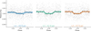 |
Fig. 1 Light curves of TOI-1468 b of individual fits. The left light curve is from visit 1, the middle light curve corresponds to visit 2, and the right light curve is from visit 3. The grey points are detrended flux measurements. The continuous lines show the best-fit occultation models, and the light coloured shaded area is the 95% HDI. Blue corresponds to visit 1, green to visit 2, and orange to visit 3. The black points show the binned data. |
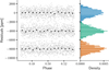 |
Fig. 2 Flux residuals of TOI-1468 b after removing trends and occultation model. In the left panel, the top residuals are from visit 1, the middle panel corresponds to visit 2, and the bottom bottom panel corresponds to visit 3. Visits 2 and 3 are offset for clarity. The grey points show residual values. The black points show the binned data. The right panel shows the residual density distribution aligned to the corresponding visit. |
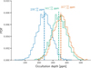 |
Fig. 3 Posterior density distribution functions for the occultation depth parameter in visit 1 (blue), visit 2 (green), and visit 3 (orange). |
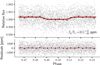 |
Fig. 4 Phase-folded light curves of TOI-1468 b. The top panel shows detrended flux measurements phase-folded at the orbital period of the panel. The grey points show the detrended flux measurements. The red line represents the best-fit joint occultation model, and the light red shaded area is the 95% highest density interval (HDI). The black dots show the binned data. The bottom panel shows the residuals in ppm after removing the best-fit model, and the dashed red line displays the zero value for clarity. |
3.3 Expected equilibrium and brightness temperature of planet b
To estimate the equilibrium temperature of the planet, we used the stellar and orbital parameters from the EXOFASTv2 fit in Table F.1, Te f f,⋆ = 3376 ± 45 K, R⋆ = 0.3714 ± 0.01 R⊙, a = 12.2 ± 0.35 R⋆, assuming zero Bond albedo, and we inserted them into Eq. (7). If the day-side of TOI-1468 b does not redistribute heat to the night-side (f = 2/3), the day-side disk-averaged temperature is Td = 874 ± 32 K. If heat is efficiently redistributed around the sphere (f = 1/4), the equilibrium temperature has a value Td = 683 ± 32 K. The latter is consistent with the reported value by Chaturvedi et al. (2022) and the global EXOFASTv2 best-fit value in Table F.1. To determine the planetary brightness temperature, we solved Eq. (6) numerically given the measured occultation depth of 311 ± 31 ppm and including the MIRI F1500W transmission function, BT-Settl stellar model, and the stellar parameters Te f f,⋆ = 3376 ± 45 K and log g=4.846 ± 0.025 (Table F.1). We used the retrieval code BeAR, which is an open-source program that performs atmospheric retrievals based on HELIOS-r2 (Kitzmann et al. 2020) with forward models in a Bayesian framework, to estimate the temperature assuming the planet as a blackbody. The best fit for the brightness temperature of the planet yields Tb = ![Mathematical equation: $\[1024_{-74}^{+78}\]$](/articles/aa/full_html/2025/06/aa53449-24/aa53449-24-eq28.png) K. Following recent works (e.g., Weiner Mansfield et al. 2024; Xue et al. 2024; Park Coy et al. 2024; August et al. 2025), we computed the ratio of the measured brightness temperature to the theoretical maximum, corresponding to no heat redistribution and zero-albedo scenario computed above. The ratio is 1.17 ± 0.10. To place this value into context of the Hot Rocks survey, for LHS 1478 b, August et al. (2025) reported a brightness temperature ratio of 0.67±0.13. In a wider context, TOI-1468 b has the highest ratio compared to other rocky exoplanets around M dwarfs observed by JWST (for more details, see Table 2 Park Coy et al. 2024).
K. Following recent works (e.g., Weiner Mansfield et al. 2024; Xue et al. 2024; Park Coy et al. 2024; August et al. 2025), we computed the ratio of the measured brightness temperature to the theoretical maximum, corresponding to no heat redistribution and zero-albedo scenario computed above. The ratio is 1.17 ± 0.10. To place this value into context of the Hot Rocks survey, for LHS 1478 b, August et al. (2025) reported a brightness temperature ratio of 0.67±0.13. In a wider context, TOI-1468 b has the highest ratio compared to other rocky exoplanets around M dwarfs observed by JWST (for more details, see Table 2 Park Coy et al. 2024).
3.4 Atmosphere
We modelled a CO2-dominated, H2O-dominated, and a mixture of 10% CO2 with 90% H2O and 90% CO2 with 10% H2O atmospheres at a surface pressure of 1 bar. The simulations were performed for surface albedos of 0.1. Figures 5 and 6 display the mean emission spectra and temperature profiles resulting from the simulations using the parametrisation reported by Koll (2022) of the heat redistribution factor and a surface pressure of 1 bar. In the case of no atmosphere, we used zero and 0.1 albedo. The scenarios without an atmosphere with 0 and 0.1 surface albedo are consistent with the observations at 1.65σ and 2σ, respectively. The cases with a CO2- or H2O-dominated atmosphere or a mix of the two species at 1 bar or above are ruled out at a significance higher than 3σ.
Among the considered models, the observations are mostly consistent with a blackbody emitter at a median temperature of 1024 K or an bare rock devoid of atmosphere. To increase the energy budget on the day-side and produce higher emission, we explored the scenario of no heat redistribution. The heat transport on tidally locked exoplanets depends on multiple mechanisms, but it strongly depends on the presence of an atmosphere (e.g., Wordsworth 2015). For instance, even a thin atmosphere can redistribute heat to some extent to the night-side (Pierrehumbert & Hammond 2019). Solid mantles, on the other hand, redistribute heat inefficiently (e.g., Meier et al. 2021). Indications of an inefficient heat redistribution on a tidally locked exoplanet have been observed on LHS 3844 b (Kreidberg et al. 2019). In this work, all models for no redistribution have an approximately 50 ppm higher emission than for full redistribution at 15 μm, but they are still slightly shallower compared to the observations (see Fig. C.1).
The features in an emission spectra are linked to changes in the temperature profile, as shown in Fig. 6. The atmospheres with lower CO2 levels are more transparent than the CO2-dominated atmosphere. A large contribution to the outgoing emission at 15 μm comes from the deeper layers of the atmosphere.
4 Discussion
The measured thermal emission is higher than expected from theoretical models. Moreover, the observed occultation is inconsistent with a cloud-free CO2 or H2O atmosphere at surface pressures above 1 bar at 15 μm. Because the effective temperature is above the day-side temperature assuming zero heat redistribution, TOI-1468 b probably is a hot and airless bare rock, which is consistent at 1.65 sigma, or a blackbody at an effective temperature of around 1024 K. The fact that Tb is slightly higher than Td might indicate an additional source of energy on the planet. We discuss the mechanisms that might cause the deep observed occultation.
4.1 Thermal inversion
If TOI-1468 b has an atmosphere, it may contain a very efficient absorber of stellar radiation. This might lead to a temperature inversion. In general, when the temperature profile becomes hotter as the pressure increases, an absorption feature is observed, but if there is a thermal inversion in the atmosphere, an emission feature is observed. If the atmosphere contains a species that efficiently absorbs the stellar radiation, an inversion might result, which would lead to a higher thermal emission. For instance, the ozone layer on Earth contributes to thermal inversion in the atmosphere. Silicate atmospheres contain different species that are strong absorbers in the IR, notably Na and SiO in lava planets (Zilinskas et al. 2022). Models show that for planets with a mass between 1 and 10 M⊕ and a surface temperature below 2096 K, the partial pressure is dominated by Na, O2, and O, while SiO dominates at a higher surface temperature (Miguel et al. 2011). The estimated temperature of 1000 K on TOI-1468 b means that SiO is rejected as possible absorber, but Na is a possible candidate for dominating the atmosphere and producing an inversion layer. Certain atmospheric conditions might lead to the formation of Na clouds. In particular, the Na condensates NaCl and Na2S are stable at surface pressures of 1 bar and above (see Fig. 3 in Marley et al. 2013). If the clouds are thick enough, they might generate variation in the surface albedo and imprint a signal on the dayside thermal emission (Castan & Menou 2011). This might explain the observed thermal emission on TOI-1468 b.
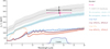 |
Fig. 5 Emission spectra for different atmospheric scenarios. The curves show the ratio of planetary to stellar flux in ppm as a function of wavelength in μm. In all cases, we considered a surface albedo of 0.1 and a heat redistribution factor based on Koll (2022) as colour-coded in the legend, ordered by the corresponding location of the model in the 15 μm bandpass. Only the no-atmosphere cases have an albedo of 0 and 0.1 and zero heat redistribution. The dashed grey line and the shaded area show the blackbody emission at 1024 K and in 1σ confidence intervals. The black dot shows the measured joint occultation depth with its 1σ uncertainty, and the pink diamond shows the measured value from the independent analysis using Frida. The blue curve and shaded light blue area at the bottom shows the response function of the F1500W filter. |
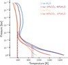 |
Fig. 6 Temperature-pressure profiles of an atmosphere at 1 bar for varying atmospheric compositions of CO2 and H2O. The different models are colour-coded in the legend. The shaded region shows the 1σ confidence interval. The vertical dashed lines depict the brightness temperature of each model at 15 μm, colour-coded except for the CO2 atmosphere for clarity. |
4.2 Induction heating
Stellar mass models (Shields et al. 2016) place the star between the partially to fully convective regime (M⊙ < 0.35). Several fully convective M dwarfs were observed to have strong magnetic fields of about 1000 G (Vidotto et al. 2014). Under special conditions, the varying magnetic field on the orbiting planet generates induction heating, which increases the energy budget. Induction heating can increase outgassing and even form subsurface magma oceans on rocky exoplanets. A necessary condition for induction heating to occur is that the normal of the orbital plane is inclined with respect to the stellar rotation axis, or that the magnetic field is misaligned to the stellar rotation axis (Kislyakova et al. 2018). It is possible that a strong variable magnetic field on TOI-1468 is heating planet b. The effect can be quantified with spectrophotometers such as SPIRou (Donati et al. 2020). Zeeman-Doppler imaging (ZDI) maps the magnetic field and its geometry, which provides evidence of induction heating. The challenge is that the rotation period of the star is about 40 days, and SPIRou cannot perform continuous observations for this long time frame. An alternative is to model the magnetohy-drodynamics of the system, which is beyond the scope of this paper.
4.3 Instrumental artefact
The origin might be at the JWST data reduction. The MIRI instrument has particular added challenges during data reduction, such as the EMI noise. Various data-processing algorithms, such as Eureka! (Bell et al. 2022), are being employed for processing JWST observations from raw data to a spectrum. The diverse approaches show that no optimal way to process JWST data exists to date. Fortunately, the scientific community has been quick to study the instrument performance and reported issues and their solutions (e.g. Dyrek et al. 2024; Libralato et al. 2024; Morrison et al. 2023). Different reduction procedures can lead to vastly different interpretations of the observations. It is plausible that the data reduction might cause the deep occultation we measured. To ensure that this is not the case, we performed three independent data reductions and analyses (only one is presented in Sect. 2.6), and we were careful to not use the same pipeline or data processing tools. The derived occultation depths agreed with each other within 2σ, and no analysis reported an occultation depth below 200 ppm. Consequently, it is unlikely that the data reduction presented in Sect. 2.2 induces the excessively deep occultation.
Another possibility is that a specific unaccounted-for source of noise in MIRI affects the observations. Visual inspection of the individual frames shows a vertical gradient on the electron counts. Specifically, the counts in the lower region of the subarray are lower and gradually increase in the vertical direction. This might not impact our analysis as the selected background region for subtraction encompasses a region far from the top and bottom. We found marginal evidence of correlated noise in the residuals (see Appendix B). Nevertheless, if multiple MIRI observations systematically yield a deeper occultation depth, a currently unaccounted-for systematic might be associated with the instrument.
4.4 Tidal heating
A possible explanation is that TOI-1468 b moves on an eccentric orbit. Notably, the orbit of TOI-1468 b might be perturbed by its transiting sibling planet TOI-1468 c. An eccentric orbit produces internal heat through the tidal effects on the planet that are caused by the star or other planets (Correia & Laskar 2010). Substantial internal energy of the planet can result as orbital energy is converted into tidal energy during the planetary evolution (Perryman 2018). A planet on an eccentric orbit will experience variable tidal forces as approaches and recedes from its host star and is periodically deformed. If the planet experiences a rapid circularisation, the dissipated energy can exceed the internal energy of the planet and might cause the planet to glow (Perryman 2018). This would translate into a higher thermal emission. For instance, GJ 876d (Rivera et al. 2005), the first discovered sub-Neptune that orbits an M4.0V star, seems to have experienced substantial tidal heating with a budget that exceeds the required power to melt a silicate mantle (Valencia et al. 2007). To challenge this hypothesis, we included the eccentricity as a free parameter in the joint fit with EXOFASTv2 (Eastman et al. 2019). However, the best-fit parameters revealed that the eccentricity for TOI-1468 b is ![Mathematical equation: $\[0.0099_{-0.005}^{+0.018}\]$](/articles/aa/full_html/2025/06/aa53449-24/aa53449-24-eq29.png) (see Table F.1) and is thus consistent with zero. We infer from this that tidal heating is probably not the explanation.
(see Table F.1) and is thus consistent with zero. We infer from this that tidal heating is probably not the explanation.
4.5 System contamination
The thermal emission from atmospheric models strongly depends on the stellar model. For instance, it is well known that M dwarfs are active stars (e.g., Diamond-Lowe et al. 2021) because flares and intense XUV activity are common. However, TOI-1468 seems to be only weakly active at optical wavelengths (Chaturvedi et al. 2022), but activity at high energies is still possible (e.g., Loyd et al. 2018). The issue is that the host star has been poorly studied in the past. Most of the stellar and orbital parameters originate from the discovery paper (Chaturvedi et al. 2022). Follow-up observations of the host star might provide insightful information for the models. Different stellar parameters affect the theoretical emission spectra and atmospheric retrieval, which might change the atmospheric composition fit to the observations of TOI-1468 b. While stellar activity might not significantly affect the temperature profile, it could influence the chemistry in the atmosphere.
The sibling transiting planet c might also contaminate the light curve of TOI-1468 b with its thermal emission. To test this, we included the thermal phase curve of TOI-1468 c using the best-fit parameters in Table F.1 in our MCMC routines. During the observations and given the long orbital period of planet c compared to the observation timescale, the thermal phase curve can be approximated by a linear function and does not affect the resulting occultation depth of TOI-1468 b. Ultimately, we found no evidence of thermal contamination by planet c.
4.6 Stellar spectrum models
Another factor related to the host star that might affect the modelled emission spectra is the stellar model. A discrepancy between the measured stellar flux and the expected flux from the stellar model indicates that an adjustment of the model is required (see e.g., Fauchez et al. 2025). If the measured flux is higher than the flux from the model, then an upscaling of the stellar spectrum translates into a lower modelled thermal emission. An excess of flux from the stellar model compared to the measurements requires a downscaling of the spectrum, which produces a higher modelled thermal emission. In our case, the measured flux and expected stellar flux using the interpolated BT_Settl model agree with each other within 0.14σ. In particular, the measured flux is 1.2 ± 6.2%, which is marginally higher than the BT_Settl model. This is similar to the results for TRAPPIST-1 c (Zieba et al. 2023), where both fluxes are consistent within 1%. In contrast, Greene et al. (2023) found a 13% excess in the measured flux of TRAPPIST-1 compared to the PHOENIX model. For our work, no rescaling is necessary, and we conclude that our BT_Settl stellar model does not cause the atmospheric models to yield a lower thermal emission compared to the observations. However, it has to be noted that our comparison only applies to the 15 μm bandpass. The stellar model can still be incorrect or require adjustment at other wavelengths, and it might thus be the source of discrepancy compared to observations.
5 Conclusions
The abundance of M dwarfs in our galaxy and the feasibility of finding and characterising a rocky exoplanet around such a star ignited interest in M dwarf systems (Bochanski et al. 2010; Gould et al. 2003; Dressing & Charbonneau 2015). There is no conclusive detection of an atmosphere around a terrestrial exoplanet orbiting an M dwarf to date. There are, however, indications of an atmosphere, such as the tentative sulphur-rich atmosphere around L 98-59 d (Banerjee et al. 2024; Gressier et al. 2024). Motivated by this issue, the Hot Rocks Survey aims to determine whether terrestrial exoplanets around M dwarfs have a thick CO2-rich atmosphere or if they are bare rocks. We presented the three observations of the occultation of TOI-1468 b (Chaturvedi et al. 2022), which is a rocky exoplanet (1.4 R⊕) that orbits an M3V dwarf.
The analysis yielded a joint occultation depth of 311 ± 31 ppm. From the individual visits, we found an occultation depth of 239 ± 52 ppm, 341 ± 53 ppm, and 357 ± 52 ppm. The derived day-side brightness temperature of ![Mathematical equation: $\[1024_{-74}^{+78}\]$](/articles/aa/full_html/2025/06/aa53449-24/aa53449-24-eq30.png) K is slightly higher than the day-side temperature without an atmosphere and zero surface albedo at 1.65σ, and it is thus statistically not significant. The atmospheric models showed that if the planet has an atmosphere, it does not have a significant amount of CO2 or H2O. It is also plausible that TOI-1468 b is a bare hot rock without an atmosphere, but this is not conclusive because the process causing the deeper-than-predicted occultation depth remains unsolved.
K is slightly higher than the day-side temperature without an atmosphere and zero surface albedo at 1.65σ, and it is thus statistically not significant. The atmospheric models showed that if the planet has an atmosphere, it does not have a significant amount of CO2 or H2O. It is also plausible that TOI-1468 b is a bare hot rock without an atmosphere, but this is not conclusive because the process causing the deeper-than-predicted occultation depth remains unsolved.
The origin of the high day-side temperature is currently unknown, but we proposed both instrumental and astrophysical hypotheses. If the signal is astrophysical in nature, this would be an intriguing result and would suggest an unaccounted-for source of energy heating the planet. If the planet harbours an atmosphere, it may possess an efficient absorber of stellar radiation, which would lead to a temperature inversion in the atmosphere and imprint a stronger signal on thermal emission. Despite the sibling transiting planet c, which might perturb the system and contribute to tidal heating on planet b, the joint fit gives a near circular orbit. This rules out tidal heating as a possibility. Because M dwarfs have been observed to have strong magnetic fields, induction heating is another possibility. Depending on the system architecture, a variable magnetic field strength due to the motion of the exoplanet can provide enough energy to even melt the surface of a rocky exoplanet (Kislyakova et al. 2018). The contribution of induction heating can be a strong source of additional energy in the exoplanet (Driscoll & Barnes 2015).
The results presented here motivate future observations at different wavelength channels; the MIRI imaging at 15 μm only provides a single photometric point. Alternatively, by measuring a full phase curve of TOI-1468 b, we can obtain precise observations of the day- and night-side emission, which would unambiguously lead to the detection of an atmosphere or would prove that there is none (Hammond et al. 2025). The work presented here shows that the Hot Rocks Survey can deepen our understanding of the atmospheres on terrestrial exoplanets around M dwarfs. The interest in these objects is reflected by the initiative to search for atmospheres of rocky M dwarf exoplanets that was recently approved by the STScI (Redfield et al. 2024). The large-scale survey will use approximately 500 hours of the director’s discretionary time on the JWST to observe about a dozen exoplanets in nearby systems, while roughly 250 HST orbits will complement the survey with UV observations to characterise the activity of the host stars. The results provided by the Hot Rocks Survey will serve as a valuable pathway for this large-scale survey.
Data availability
The raw and detrended photometric time-series data are available in electronic form at the CDS via anonymous ftp to cdsarc.cds.unistra.fr (130.79.128.5) or via https://cdsarc.cds.unistra.fr/viz-bin/cat/J/A+A/698/A68
Acknowledgements
We are grateful to the anonymous referee for the careful reading and thoughtful suggestions that improved this paper. Based on observations with the NASA/ESA/CSA James Webb Space Telescope obtained at the Space Telescope Science Institute, which is operated by the Association of Universities for Research in Astronomy, Incorporated, under NASA contract NAS5-03127. E.M.V. acknowledges support from the Centre for Space and Habitability (CSH). This work has been carried out within the framework of the National Centre of Competence in Research PlanetS supported by the Swiss National Science Foundation under grant 51NF40_205606. E.M.V. acknowledges financial support from the Swiss National Science Foundation (SNSF) Postdoc.Mobility Fellowship under grant no. P500PT_225456/1. B.-O.D. acknowledges support from the Swiss State Secretariat for Education, Research and Innovation (SERI) under contract number MB22.00046. H.D.L. and P.C.A. acknowledges support from the Carlsberg Foundation, grant CF221254. J.M.M. acknowledges support from the Horizon Europe Guarantee Fund, grant EP/Z00330X/1. N.H.A. acknowledges support by the National Science Foundation Graduate Research Fellowship under Grant No. DGE1746891. C.E.F. acknowledges support from the European Research Council (ERC) under the European Union’s Horizon 2020 research and innovation program under grant agreement no. 805445. N.P.G. gratefully acknowledges support from Science Foundation Ireland and the Royal Society through a University Research Fellowship (URF\textbackslash R\textbackslash 201032). H.J.H. acknowledges support from eSSENCE (grant number eSSENCE@LU 9:3), The Crafoord foundation and the Royal Physiographic Society of Lund, through The Fund of the Walter Gyllenberg Foundation. B.P. acknowledges support from the Walter Gyllenberg Foundation. A.D.R. acknowledges support from the Carlsberg Foundation, grant CF22-1548. We acknowledge the input from the following individuals to the GO 3730 proposal: Can Akin, Andrea Guzman Mesa, Nicholas Borsato, Adam Burgasser, Meng Tian, Mette Baungaard. We thank Dr. Yamila Miguel for insightful discussions on atmospheric thermal inversion. We thank Dr. Jen Winters for important conversations on the potential multiplicity of the host star. The authors thank Suzanne Aigrain for discussions on stellar activity and data analysis. This research made use of exoplanet (Foreman-Mackey et al. 2021) and its dependencies (Agol et al. 2020; Kumar et al. 2019; Astropy Collaboration 2013, 2018; Kipping 2013; Luger et al. 2019; Salvatier et al. 2016; Theano Development Team 2016). We acknowledge the use of further software: batman (Kreidberg 2015), NumPy (Harris et al. 2020), matplotlib (Hunter 2007), corner (Foreman-Mackey 2016), astroquery (Ginsburg et al. 2019) and scipy (Virtanen et al. 2020). This work made use of seaborn (Waskom 2021) to generate the colourblind palette.
Appendix A Raw photometry
We present the absolute measurements for each visit before normalising. The average absolute flux is in visit 1,2 and 3, respectively. Overall, the values are as expected for the target, as reported in Sect. 3.1.
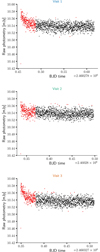 |
Fig. A.1 Raw photometry for visit 1 (top), visit 2 (middle) and visit 3 (bottom) in units of mJy as a function of time. Red data points are discarded data points as described in Sect. 2.3. |
Appendix B Allan variance plots
Here we present the root mean square (RMS) of the residual measurements as a function of bin size. In the absence of correlated noise, the residual RMS decreases as 1/ ![Mathematical equation: $\[\sqrt{n}\]$](/articles/aa/full_html/2025/06/aa53449-24/aa53449-24-eq31.png) , where n is the size of the bin. The resulting Allan variance plots (Allan 1966) of the residuals for each visit are shown in Fig. B.1. As mentioned in Sec. 2.3, the detrending models for all visits consist of a linear trend in time and background.
, where n is the size of the bin. The resulting Allan variance plots (Allan 1966) of the residuals for each visit are shown in Fig. B.1. As mentioned in Sec. 2.3, the detrending models for all visits consist of a linear trend in time and background.
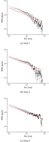 |
Fig. B.1 Photometric residual RMS as a function of bin size in minutes. The red dashed line shows the expected Poissonian noise precision normalised to the unbinned RMS. The panel on the left corresponds to visit 1, the middle panel to visit 2 and the right panel to visit 3. |
Appendix C Atmospheric models for heat redistribution boundary scenarios
We present the atmospheric models for the cases of no heat redistribution to the nightside (f=2/3) and full heat redistribution (f=1/4) described in Sect. 2.5 for a pure CO2 atmosphere, pure H2O, 10% CO2 and 90% H2O and 90% CO2 and 10% H2O atmosphere. In all cases the surface albedo and pressure are 0.1 and 1000 mbar, respectively.
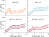 |
Fig. C.1 Emission spectra for different atmospheric scenarios. The curves show the planetary flux to stellar flux ratio in ppm as a function of wavelength in μm. Each panel corresponds to the atmospheric composition labelled on the top of the panel. In each panel, the top curve represents the model for no heat redistribution (f=2/3), while the bottom curve is for full redistribution (f=1/4). The shaded area covers the scenarios in between the boundary cases. |
Appendix D Analysis for different aperture sizes
Here we present the analysis following Sect. 2 for apertures between 3 and 20 pixels for photometric extraction. In each case, we compute the MAD of the raw light-curve and for the trimmed data after removing the first segment, the posterior estimate on the occultation depth and the residual RMS. The resulting values are presented in Table D.1. The selection of aperture size for the main analysis is based on these values. In all cases, the background annulus was fixed with an inner radius of 30 pixels and outer radius of 50 pixels.
Analysis for different aperture sizes.
Appendix E Corner plot of the joint analysis
Figure E.1 shows the full joint posterior correlation plots of the joint analysis. a0,j is the mean flux, a1,j the slope of the linear trend in time and a6,j the background level of visit j with j ∈ {1, 2, 3}; Rs and Ms are the stellar radius and mass, T0 is the mid-transit time, P the orbital period, Rp/Rs is the ratio of the planetary radius to the stellar radius, b is the impact parameter, fp/ fs the occultation depth, and log(s) is the natural logarithm of the flux uncertainty for each measurement.
 |
Fig. E.1 Posterior distributions and joint correlations plot corresponding to to joint analysis of TOI-1468 b observations. |
Appendix F EXOFASTv2 global fit
Table F.1 presents the best-fit parameters of the global fit performed with EXOFASTv2 (Eastman et al. 2019) described in Sect. 2.3.
EXOFASTv2 median values and 68% confidence interval for TOI-1468.
References
- Agol, E., Luger, R., & Foreman-Mackey, D. 2020, AJ, 159, 123 [Google Scholar]
- Alam, M. K., Gao, P., Adams Redai, J., et al. 2024, AJ, 169, 15 [Google Scholar]
- Allan, D. 1966, Proceedings of the IEEE, 54, 221 [Google Scholar]
- Allard, F., Homeier, D., & Freytag, B. 2011, ASP Conf. Ser., 448, 91 [Google Scholar]
- Allard, F., Homeier, D., & Freytag, B. 2012, Phil. Trans. R. Soc. London Ser. A, 370, 2765 [Google Scholar]
- Astropy Collaboration (Robitaille, T. P., et al.) 2013, A&A, 558, A33 [NASA ADS] [CrossRef] [EDP Sciences] [Google Scholar]
- Astropy Collaboration (Price-Whelan, A. M., et al.) 2018, AJ, 156, 123 [Google Scholar]
- August, P. C., Buchhave, L. A., Diamond-Lowe, H., et al. 2025, A&A, 695, A171 [NASA ADS] [CrossRef] [EDP Sciences] [Google Scholar]
- Banerjee, A., Barstow, J. K., Gressier, A., et al. 2024, ApJ, 975, L11 [Google Scholar]
- Barber, R. J., Tennyson, J., Harris, G. J., & Tolchenov, R. N. 2006, MNRAS, 368, 1087 [Google Scholar]
- Barman, T. S., Hauschildt, P. H., & Allard, F. 2005, ApJ, 632, 1132 [Google Scholar]
- Bell, T., Ahrer, E.-M., Brande, J., et al. 2022, JOSS, 7, 4503 [Google Scholar]
- Bell, T. J., Crouzet, N., Cubillos, P. E., et al. 2024, Nat. Astron., 8, 879 [Google Scholar]
- Bello-Arufe, A., Damiano, M., Bennett, K. A., et al. 2025, ApJ, 980, L26 [Google Scholar]
- Bochanski, J. J., Hawley, S. L., Covey, K. R., et al. 2010, AJ, 139, 2679 [NASA ADS] [CrossRef] [Google Scholar]
- Borucki, W. J., Koch, D., Basri, G., et al. 2010, Science, 327, 977 [Google Scholar]
- Bradley, L., Sipőcz, B., Robitaille, T., et al. 2022, https://doi.org/10.5281/zenodo.6825092 [Google Scholar]
- Burrows, A. S. 2014, PNAS, 111, 12601 [NASA ADS] [CrossRef] [Google Scholar]
- Castan, T., & Menou, K. 2011, ApJ, 743, L36 [NASA ADS] [CrossRef] [Google Scholar]
- Chaturvedi, P., Bluhm, P., Nagel, E., et al. 2022, A&A, 666, A155 [NASA ADS] [CrossRef] [EDP Sciences] [Google Scholar]
- Correia, A. C. M., & Laskar, J. 2010, in Exoplanets, ed. S. Seager (Berlin: Springer), 239 [Google Scholar]
- Cowan, N. B., & Agol, E. 2010, ApJ, 726, 82 [Google Scholar]
- Cox, A. N. 2000, Allen’s Astrophysical Quantities (Berlin: Springer) [Google Scholar]
- Crossfield, I. J. M., Waalkes, W., Newton, E. R., et al. 2019, ApJ, 883, L16 [Google Scholar]
- Crossfield, I. J. M., Malik, M., Hill, M. L., et al. 2022, ApJ, 937, L17 [NASA ADS] [CrossRef] [Google Scholar]
- Damiano, M., Hu, R., Barclay, T., et al. 2022, AJ, 164, 225 [Google Scholar]
- de Wit, J., Wakeford, H. R., Lewis, N. K., et al. 2018, Nat. Astron., 2, 214 [NASA ADS] [CrossRef] [Google Scholar]
- Delrez, L., Gillon, M., Queloz, D., et al. 2018, SPIE, 10700, 446 [Google Scholar]
- Diamond-Lowe, H., Berta-Thompson, Z., Charbonneau, D., & Kempton, E. M. R. 2018, AJ, 156, 42 [NASA ADS] [CrossRef] [Google Scholar]
- Diamond-Lowe, H., Charbonneau, D., Malik, M., Kempton, E. M. R., & Beletsky, Y. 2020, AJ, 160, 188 [NASA ADS] [CrossRef] [Google Scholar]
- Diamond-Lowe, H., Youngblood, A., Charbonneau, D., et al. 2021, AJ, 162, 10 [NASA ADS] [CrossRef] [Google Scholar]
- Diamond-Lowe, H., Mendonca, J. M., Akin, C. J., et al. 2023a, The Hot Rocks Survey: Testing 9 Irradiated Terrestrial Exoplanets for Atmospheres (USA: JWST Proposal. Cycle 2, ID.), 3730 [Google Scholar]
- Diamond-Lowe, H., Mendonça, J. M., Charbonneau, D., & Buchhave, L. A. 2023b, AJ, 165, 169 [NASA ADS] [CrossRef] [Google Scholar]
- Dietrich, J., Apai, D., Schlecker, M., et al. 2023, AJ, 165, 149 [NASA ADS] [CrossRef] [Google Scholar]
- Donati, J. F., Kouach, D., Moutou, C., et al. 2020, MNRAS, 498, 5684 [Google Scholar]
- Dressing, C. D., & Charbonneau, D. 2015, ApJ, 807, 45 [Google Scholar]
- Driscoll, P. E., & Barnes, R. 2015, Astrobiology, 15, 739 [NASA ADS] [CrossRef] [Google Scholar]
- Ducrot, E., Lagage, P.-O., Min, M., et al. 2025, Nat. Astron., 9, 358 [Google Scholar]
- Dyrek, A., Ducrot, E., Lagage, P. O., et al. 2024, A&A, 683, A212 [NASA ADS] [CrossRef] [EDP Sciences] [Google Scholar]
- Eastman, J. D., Rodriguez, J. E., Agol, E., et al. 2019, PASP, submitted [arXiv:1907.09480] [Google Scholar]
- Eschen, Y. N. E., & Kunimoto, M. 2024, MNRAS, 531, 5053 [Google Scholar]
- Essack, Z., Seager, S., & Pajusalu, M. 2020, ApJ, 898, 160 [CrossRef] [Google Scholar]
- Fauchez, T. J., Rackham, B. V., Ducrot, E., Stevenson, K. B., & de Wit, J. 2025, ApJ, submitted [arXiv:2502.19585] [Google Scholar]
- Foreman-Mackey, D. 2016, JOSS, 1, 24 [NASA ADS] [CrossRef] [Google Scholar]
- Foreman-Mackey, D., Savel, A., Luger, R., et al. 2021, https://doi.org/10.5281/zenodo.1998447 [Google Scholar]
- Fortune, M., Gibson, N. P., & Diamond-Lowe, H. 2025, A&A, submitted [Google Scholar]
- Fulton, B. J., Petigura, E. A., Howard, A. W., et al. 2017, AJ, 154, 109 [Google Scholar]
- Garraffo, C., Drake, J. J., & Cohen, O. 2016, ApJ, 833, L4 [NASA ADS] [CrossRef] [Google Scholar]
- Garraffo, C., Drake, J. J., Cohen, O., Alvarado-Gómez, J. D., & Moschou, S. P. 2017, ApJ, 843, L33 [Google Scholar]
- Gelman, A., & Rubin, D. B. 1992, Stat. Sci., 7, 457 [Google Scholar]
- Gibbs, A., Bixel, A., Rackham, B. V., et al. 2020, AJ, 159, 169 [NASA ADS] [CrossRef] [Google Scholar]
- Gilbert, E. A., Barclay, T., Schlieder, J. E., et al. 2020, AJ, 160, 116 [Google Scholar]
- Gillon, M., Jehin, E., Fumel, A., Magain, P., & Queloz, D. 2013, EPJ Web Conf., 47, 03001 [NASA ADS] [CrossRef] [EDP Sciences] [Google Scholar]
- Gillon, M., Jehin, E., Lederer, S. M., et al. 2016, Nature, 533, 221 [Google Scholar]
- Gillon, M., Pedersen, P. P., Rackham, B. V., et al. 2024, Nat. Astron., 8, 865 [Google Scholar]
- Ginsburg, A., Sipőcz, B. M., Brasseur, C. E., et al. 2019, AJ, 157, 98 [Google Scholar]
- Gordon, K. D., Sloan, G. C., Garcia Marin, M., et al. 2025, AJ, 169, 6 [Google Scholar]
- Gould, A., Pepper, J., & DePoy, D. L. 2003, ApJ, 594, 533 [Google Scholar]
- Greene, T. P., Bell, T. J., Ducrot, E., et al. 2023, Nature, 618, 39 [NASA ADS] [CrossRef] [Google Scholar]
- Gressier, A., Espinoza, N., Allen, N. H., et al. 2024, ApJ, 975, L10 [NASA ADS] [CrossRef] [Google Scholar]
- Grimm, S. L., Malik, M., Kitzmann, D., et al. 2021, ApJS, 253, 30 [NASA ADS] [CrossRef] [Google Scholar]
- Günther, M. N., Pozuelos, F. J., Dittmann, J. A., et al. 2019, Nat. Astron., 3, 1099 [Google Scholar]
- Hammond, M., Guimond, C. M., Lichtenberg, T., et al. 2025, ApJ, 978, L40 [Google Scholar]
- Hansen, B. M. S. 2008, ApJS, 179, 484 [NASA ADS] [CrossRef] [Google Scholar]
- Harris, C. R., Millman, K. J., van der Walt, S. J., et al. 2020, Nature, 585, 357 [NASA ADS] [CrossRef] [Google Scholar]
- Hoffman, M. D., & Gelman, A. 2011, J. Mach. Learn. Res., 15, 1593 [Google Scholar]
- Hu, R., Bello-Arufe, A., Zhang, M., et al. 2024, Nature, 630, 609 [NASA ADS] [CrossRef] [Google Scholar]
- Hunter, J. D. 2007, Comput. Sci. Eng., 9, 90 [NASA ADS] [CrossRef] [Google Scholar]
- Ih, J., Kempton, E. M. R., Whittaker, E. A., & Lessard, M. 2023, ApJ, 952, L4 [CrossRef] [Google Scholar]
- Jehin, E., Gillon, M., Queloz, D., et al. 2018, The Messenger, 174, 2 [NASA ADS] [Google Scholar]
- Kipping, D. M. 2013, MNRAS, 435, 2152 [Google Scholar]
- Kislyakova, K. G., Fossati, L., Johnstone, C. P., et al. 2018, ApJ, 858, 105 [NASA ADS] [CrossRef] [Google Scholar]
- Kitzmann, D., Heng, K., Oreshenko, M., et al. 2020, ApJ, 890, 174 [Google Scholar]
- Koll, D. D. B. 2022, ApJ, 924, 134 [NASA ADS] [CrossRef] [Google Scholar]
- Kreidberg, L. 2015, PASP, 127, 1161 [Google Scholar]
- Kreidberg, L., Koll, D. D. B., Morley, C., et al. 2019, Nature, 573, 87 [NASA ADS] [CrossRef] [Google Scholar]
- Kumar, R., Carroll, C., Hartikainen, A., & Martin, O. A. 2019, J. Open Source Softw., 4, 1143 [NASA ADS] [CrossRef] [Google Scholar]
- Libby-Roberts, J. E., Berta-Thompson, Z. K., Diamond-Lowe, H., et al. 2022, AJ, 164, 59 [NASA ADS] [CrossRef] [Google Scholar]
- Libralato, M., Argyriou, I., Dicken, D., et al. 2024, PASP, 136, 034502 [Google Scholar]
- Lim, O., Benneke, B., Doyon, R., et al. 2023, ApJ, 955, L22 [NASA ADS] [CrossRef] [Google Scholar]
- Loyd, R. O. P., France, K., Youngblood, A., et al. 2018, ApJ, 867, 71 [Google Scholar]
- Luger, R., Agol, E., Foreman-Mackey, D., et al. 2019, AJ, 157, 64 [Google Scholar]
- Lustig-Yaeger, J., Fu, G., May, E. M., et al. 2023, Nat. Astron., 7, 1317 [NASA ADS] [CrossRef] [Google Scholar]
- Malik, M., Grosheintz, L., Mendonça, J. M., et al. 2017, AJ, 153, 56 [Google Scholar]
- Malik, M., Kempton, E. M. R., Koll, D. D. B., et al. 2019a, ApJ, 886, 142 [NASA ADS] [CrossRef] [Google Scholar]
- Malik, M., Kitzmann, D., Mendonça, J. M., et al. 2019b, AJ, 157, 170 [Google Scholar]
- Mallonn, M., Köhler, J., Alexoudi, X., et al. 2019, A&A, 624, A62 [NASA ADS] [CrossRef] [EDP Sciences] [Google Scholar]
- Mandel, K., & Agol, E. 2002, ApJ, 580, L171 [Google Scholar]
- Marley, M. S., Ackerman, A. S., Cuzzi, J. N., & Kitzmann, D. 2013, in Comparative Climatology of Terrestrial Planets, eds. S. J. Mackwell, A. A. Simon-Miller, J. W. Harder, & M. A. Bullock (Tucson: University of Arizona Press), 367 [Google Scholar]
- May, E. M., MacDonald, R. J., Bennett, K. A., et al. 2023, ApJ, 959, L9 [CrossRef] [Google Scholar]
- McElreath, R. 2016, Statistical Rethinking: A Bayesian Course with Examples in R and Stan, Chapman & Hall/CRC Texts in Statistical Science (Boca Raton: CRC Press) [Google Scholar]
- Meier, T. G., Bower, D. J., Lichtenberg, T., Tackley, P. J., & Demory, B.-O. 2021, ApJ, 908, L48 [NASA ADS] [CrossRef] [Google Scholar]
- Meier Valdés, E. A., Morris, B. M., Wells, R. D., Schanche, N., & Demory, B.-O. 2022, A&A, 663, A95 [NASA ADS] [CrossRef] [EDP Sciences] [Google Scholar]
- Meier Valdés, E. A., Morris, B. M., Demory, B. O., et al. 2023, A&A, 677, A112 [NASA ADS] [CrossRef] [EDP Sciences] [Google Scholar]
- Miguel, Y., Kaltenegger, L., Fegley, B., & Schaefer, L. 2011, ApJ, 742, L19 [NASA ADS] [CrossRef] [Google Scholar]
- Moran, S. E., Stevenson, K. B., Sing, D. K., et al. 2023, ApJ, 948, L11 [NASA ADS] [CrossRef] [Google Scholar]
- Morrison, J. E., Dicken, D., Argyriou, I., et al. 2023, PASP, 135, 075004 [NASA ADS] [CrossRef] [Google Scholar]
- Nutzman, P., & Charbonneau, D. 2008, PASP, 120, 317 [Google Scholar]
- Owen, J. E. 2019, Ann. Rev. Earth Planet. Sci., 47, 67 [Google Scholar]
- O’Sullivan, N. K., & Aigrain, S. 2024, MNRAS, 531, 4181 [Google Scholar]
- Park Coy, B., Ih, J., Kite, E. S., et al. 2024, ApJ, submitted [arXiv:2412.06573] [Google Scholar]
- Patel, J. A., Brandeker, A., Kitzmann, D., et al. 2024, A&A, 690, A159 [NASA ADS] [CrossRef] [EDP Sciences] [Google Scholar]
- Perryman, M. 2018, The Exoplanet Handbook (Cambridge: Cambridge University Press) [Google Scholar]
- Pierrehumbert, R. T., & Hammond, M. 2019, Ann. Rev. Fluid Mech., 51, 275 [NASA ADS] [CrossRef] [Google Scholar]
- Pont, F., Knutson, H., Gilliland, R. L., Moutou, C., & Charbonneau, D. 2008, MNRAS, 385, 109 [Google Scholar]
- Pontoppidan, K. M., Pickering, T. E., Laidler, V. G., et al. 2016, SPIE, 9910, 991016 [Google Scholar]
- Powell, D., Feinstein, A. D., Lee, E. K. H., et al. 2024, Nature, 626, 979 [NASA ADS] [CrossRef] [Google Scholar]
- Quirrenbach, A., Amado, P. J., Caballero, J. A., et al. 2014, SPIE Conf. Ser., 9147, 91471F [Google Scholar]
- Rackham, B., Espinoza, N., Apai, D., et al. 2017, ApJ, 834, 151 [Google Scholar]
- Rajpurohit, A. S., Reylé, C., Allard, F., et al. 2013, A&A, 556, A15 [NASA ADS] [CrossRef] [EDP Sciences] [Google Scholar]
- Redfield, S., Batalha, N., Benneke, B., et al. 2024, arXiv e-prints [arXiv:2404.02932] [Google Scholar]
- Ricker, G. R., Winn, J. N., Vanderspek, R., et al. 2015, JATIS, 1, 014003 [Google Scholar]
- Rivera, E. J., Lissauer, J. J., Butler, R. P., et al. 2005, ApJ, 634, 625 [Google Scholar]
- Rothman, L. S., Gordon, I. E., Barber, R. J., et al. 2010, J. Quant. Spec. Radiat. Transf., 111, 2139 [NASA ADS] [CrossRef] [Google Scholar]
- Salvatier, J., Wiecki, T. V., & Fonnesbeck, C. 2016, PeerJ Comp. Sci., 2, e55 [CrossRef] [Google Scholar]
- Schlawin, E., Leisenring, J., Misselt, K., et al. 2020, AJ, 160, 231 [NASA ADS] [CrossRef] [Google Scholar]
- Schwarz, G. 1978, Ann. Stat., 6, 461 [Google Scholar]
- Segura, A., Walkowicz, L. M., Meadows, V., Kasting, J., & Hawley, S. 2010, Astrobiology, 10, 751 [Google Scholar]
- Seifahrt, A., Stürmer, J., Bean, J. L., & Schwab, C. 2018, SPIE Conf. Ser., 10702, 107026D [NASA ADS] [Google Scholar]
- Shields, A. L., Ballard, S., & Johnson, J. A. 2016, Phys. Rep., 663, 1 [NASA ADS] [CrossRef] [Google Scholar]
- Smithsonian Astrophysical Observatory 2000, Astrophysics Source Code Library [record ascl:0003.002] [Google Scholar]
- Sneep, M., & Ubachs, W. 2005, J. Quant. Spec. Radiat. Transf., 92, 293 [NASA ADS] [CrossRef] [Google Scholar]
- Tamburo, P., Muirhead, P. S., McCarthy, A. M., et al. 2022, AJ, 163, 253 [NASA ADS] [CrossRef] [Google Scholar]
- Tamburo, P., Muirhead, P. S., McCarthy, A. M., et al. 2022, AJ, 164, 252 [Google Scholar]
- Tarter, J. C., Backus, P. R., Mancinelli, R. L., et al. 2007, Astrobiology, 7, 30 [NASA ADS] [CrossRef] [Google Scholar]
- Thalman, R., Zarzana, K. J., Tolbert, M. A., & Volkamer, R. 2014, J. Quant. Spec. Radiat. Transf., 147, 171 [NASA ADS] [CrossRef] [Google Scholar]
- Theano Development Team (Al-Rfou, R., et al.) 2016, arXiv e-prints [arXiv:1605.02688] [Google Scholar]
- Tian, F. 2009, ApJ, 703, 905 [NASA ADS] [CrossRef] [Google Scholar]
- Tian, M., & Heng, K. 2024, ApJ, 963, 157 [NASA ADS] [CrossRef] [Google Scholar]
- Valencia, D., Sasselov, D. D., & O’Connell, R. J. 2007, ApJ, 656, 545 [Google Scholar]
- Vehtari, A., Gelman, A., & Gabry, J. 2016, Stat. Comput., 27, 1413 [Google Scholar]
- Vidotto, A. A., Jardine, M., Morin, J., et al. 2013, A&A, 557, A67 [NASA ADS] [CrossRef] [EDP Sciences] [Google Scholar]
- Vidotto, A. A., Gregory, S. G., Jardine, M., et al. 2014, MNRAS, 441, 2361 [Google Scholar]
- Virtanen, P., Gommers, R., Oliphant, T. E., et al. 2020, Nat. Methods, 17, 261 [Google Scholar]
- Wachiraphan, P., Berta-Thompson, Z. K., Diamond-Lowe, H., et al. 2024, AJ, submitted [arXiv:2410.10987] [Google Scholar]
- Waskom, M. L. 2021, JOSS, 6, 3021 [NASA ADS] [CrossRef] [Google Scholar]
- Weiner Mansfield, M., Xue, Q., Zhang, M., et al. 2024, ApJ, 975, L22 [NASA ADS] [CrossRef] [Google Scholar]
- Winn, J. N., Matthews, J. M., Dawson, R. I., et al. 2011, ApJ, 737, L18 [Google Scholar]
- Wordsworth, R. 2015, ApJ, 806, 180 [NASA ADS] [CrossRef] [Google Scholar]
- Xue, Q., Bean, J. L., Zhang, M., et al. 2024, ApJ, 973, L8 [NASA ADS] [CrossRef] [Google Scholar]
- Yao, Y., Vehtari, A., Simpson, D., & Gelman, A. 2018, Bayesian Anal., 13, 917 [Google Scholar]
- Zhang, M., Hu, R., Inglis, J., et al. 2024, ApJ, 961, L44 [NASA ADS] [CrossRef] [Google Scholar]
- Zieba, S., Kreidberg, L., Ducrot, E., et al. 2023, Nature, 620, 746 [NASA ADS] [CrossRef] [Google Scholar]
- Zilinskas, M., van Buchem, C. P. A., Miguel, Y., et al. 2022, A&A, 661, A126 [NASA ADS] [CrossRef] [EDP Sciences] [Google Scholar]
JWST observations can be downloaded on the MAST portal at https://mast.stsci.edu/portal/Mashup/Clients/Mast/Portal.html
All Tables
All Figures
|
Fig. 1 Light curves of TOI-1468 b of individual fits. The left light curve is from visit 1, the middle light curve corresponds to visit 2, and the right light curve is from visit 3. The grey points are detrended flux measurements. The continuous lines show the best-fit occultation models, and the light coloured shaded area is the 95% HDI. Blue corresponds to visit 1, green to visit 2, and orange to visit 3. The black points show the binned data. |
| In the text | |
|
Fig. 2 Flux residuals of TOI-1468 b after removing trends and occultation model. In the left panel, the top residuals are from visit 1, the middle panel corresponds to visit 2, and the bottom bottom panel corresponds to visit 3. Visits 2 and 3 are offset for clarity. The grey points show residual values. The black points show the binned data. The right panel shows the residual density distribution aligned to the corresponding visit. |
| In the text | |
|
Fig. 3 Posterior density distribution functions for the occultation depth parameter in visit 1 (blue), visit 2 (green), and visit 3 (orange). |
| In the text | |
|
Fig. 4 Phase-folded light curves of TOI-1468 b. The top panel shows detrended flux measurements phase-folded at the orbital period of the panel. The grey points show the detrended flux measurements. The red line represents the best-fit joint occultation model, and the light red shaded area is the 95% highest density interval (HDI). The black dots show the binned data. The bottom panel shows the residuals in ppm after removing the best-fit model, and the dashed red line displays the zero value for clarity. |
| In the text | |
|
Fig. 5 Emission spectra for different atmospheric scenarios. The curves show the ratio of planetary to stellar flux in ppm as a function of wavelength in μm. In all cases, we considered a surface albedo of 0.1 and a heat redistribution factor based on Koll (2022) as colour-coded in the legend, ordered by the corresponding location of the model in the 15 μm bandpass. Only the no-atmosphere cases have an albedo of 0 and 0.1 and zero heat redistribution. The dashed grey line and the shaded area show the blackbody emission at 1024 K and in 1σ confidence intervals. The black dot shows the measured joint occultation depth with its 1σ uncertainty, and the pink diamond shows the measured value from the independent analysis using Frida. The blue curve and shaded light blue area at the bottom shows the response function of the F1500W filter. |
| In the text | |
|
Fig. 6 Temperature-pressure profiles of an atmosphere at 1 bar for varying atmospheric compositions of CO2 and H2O. The different models are colour-coded in the legend. The shaded region shows the 1σ confidence interval. The vertical dashed lines depict the brightness temperature of each model at 15 μm, colour-coded except for the CO2 atmosphere for clarity. |
| In the text | |
|
Fig. A.1 Raw photometry for visit 1 (top), visit 2 (middle) and visit 3 (bottom) in units of mJy as a function of time. Red data points are discarded data points as described in Sect. 2.3. |
| In the text | |
|
Fig. B.1 Photometric residual RMS as a function of bin size in minutes. The red dashed line shows the expected Poissonian noise precision normalised to the unbinned RMS. The panel on the left corresponds to visit 1, the middle panel to visit 2 and the right panel to visit 3. |
| In the text | |
|
Fig. C.1 Emission spectra for different atmospheric scenarios. The curves show the planetary flux to stellar flux ratio in ppm as a function of wavelength in μm. Each panel corresponds to the atmospheric composition labelled on the top of the panel. In each panel, the top curve represents the model for no heat redistribution (f=2/3), while the bottom curve is for full redistribution (f=1/4). The shaded area covers the scenarios in between the boundary cases. |
| In the text | |
|
Fig. E.1 Posterior distributions and joint correlations plot corresponding to to joint analysis of TOI-1468 b observations. |
| In the text | |
Current usage metrics show cumulative count of Article Views (full-text article views including HTML views, PDF and ePub downloads, according to the available data) and Abstracts Views on Vision4Press platform.
Data correspond to usage on the plateform after 2015. The current usage metrics is available 48-96 hours after online publication and is updated daily on week days.
Initial download of the metrics may take a while.